


Introduction
Late watergrass (Echinochloa phyllopogon (Stapf.) Koss; synonym Echinochloa oryzicola Vasinger) is one of the most competitive weeds in the California rice agroecosystem, reducing yields up to 59% when uncontrolled (Gibson et al. Reference Gibson, Fischer, Foin and Hill2002). Recent data suggest that losses may be higher in dry-seeded systems (Brim-DeForest et al. Reference Brim-DeForest, Al-Khatib, Linquist and Fischer2017). In California, late watergrass germinates and emerges under both aerobic and anaerobic conditions (Boddy et al. Reference Boddy, Bradford and Fischer2012a; Linquist et al. Reference Linquist, Fischer, Godfrey, Greer, Hill and Koffler2008; Pittelkow et al. Reference Pittelkow, Fischer, Moechnig, Hill, Koffler, Mutters, Greer, Cho, van Kessel and Linquist2012). Late watergrass populations in California have evolved nontarget site–based resistance mechanisms to five modes of action (Fischer et al. Reference Fischer, Ateh, Bayer and Hill2000a, Reference Fischer, Bayer, Carriere, Ateh and Yim2000b; Yasuor et al. Reference Yasuor, TenBrook, Tjeerdem and Fischer2008; Yun et al. Reference Yun, Yogo, Yamasue and Fischer2005), and the populations are widespread throughout the California rice agroecosystem (Tsuji et al. Reference Tsuji, Fischer, Yoshino, Roel, Hill and Yamasue2003).
The management of weeds through cultural practices, including tillage and water management, is currently thought to be the best approach to managing herbicide resistance in the long term (Buhler Reference Buhler2002; Mortensen et al. Reference Mortensen, Egan, Maxwell, Ryan and Smith2012). However, one of the impediments to farmer adoption of different cultural practices is uncertainty of outcome, both in terms of level and consistency of weed control. For rice farmers, the dynamics of weed populations under new irrigation and tillage systems are often unknown, so adoption of these practices can be low. Weeds are the greatest yield constraint to rice worldwide (Zhang Reference Zhang, Auld and Kim1996), but changing farmer practices can be difficult, without first understanding the consequences to specific weed species and weed populations. Thus, in order to effectively control weeds under a variety of irrigation and tillage methods, it is first necessary to understand the effects of these practices on the emergence and early growth of each weed species in the agroecosystem.
For application of both cultural controls and herbicides, predicting emergence and early growth can be an effective tool for farmers to better time management practices. Models that have been used to predict timing of emergence of weed species include population-based threshold models (PBTM; Boddy et al. Reference Boddy, Bradford and Fischer2012a; Grundy et al. Reference Grundy, Phelps, Reader and Burston2000). PBTMs have been developed using water potential (Bradford Reference Bradford, Kigel and Galili1995; Gummerson Reference Gummerson1986), temperature (Garcia-Huidobro et al. Reference Garcia-Huidobro, Monteith and Squire1982), and oxygen (Boddy et al. Reference Boddy, Bradford and Fischer2012a; Bradford et al. Reference Bradford, Come and Corbineau2007) as parameters. The models are based on the principle that there is a minimum temperature, water potential, and oxygen, below which developmental processes cease. Predicting emergence depends on the degree of seed dormancy, soil water potential, soil temperature, oxygenation, and burial depth (Bewley et al. Reference Bewley, Bradford, Hilhorst and Nonogaki2012; Forcella et al. Reference Forcella, Benech-Arnold, Sanchez and Ghersa2000), but combining all of these aspects into one model is difficult.
Boddy et al. (Reference Boddy, Bradford and Fischer2012a) developed parameters for a hydrothermal model for late watergrass, combining temperature and water potential for both resistant (R) and susceptible (S) biotypes. They applied the models to predict germination and emergence to a shoot height of 4.5 cm above the soil surface. They found little difference between R and S biotypes in germination response to temperature, water potential, or oxygen. For emergence, R biotypes were found to be less tolerant of intermittent soil drying than S biotypes. At maturity, Boddy et al. (Reference Boddy, Streibig, Yamasue and Fischer2012b) found significant differences in fecundity and seed shattering between R and S biotypes. R biotypes produced less seed, but shattered earlier than S biotypes. They also reached anthesis earlier than S biotypes, under saturated soil conditions.
Application of the late watergrass PBTM emergence model (Boddy et al. Reference Boddy, Bradford and Fischer2012a) in the field for the susceptible (HR[S]) biotype failed to accurately predict emergence (Brim-DeForest et al. Reference Brim-DeForest, Pedroso, Boddy, Linquist and Fischer2014). Two significant factors may have contributed to the lack of fit: the assumption that seeds emerged from a normal distribution of soil depths and the assumption that early emergence was driven solely by temperature, not moisture. Other studies on multiple weed species indicate that emergence varies with depth, often decreasing with deeper burial (Benvenuti et al. Reference Benvenuti, MacChia and Miele2001). Grundy et al. (Reference Grundy, Mead and Burston2003) found that for many species, percent emergence by depth can be defined as a polynomial relationship in saturated soils, with some decrease in emergence at shallow depths, and optimal emergence below the soil surface decreasing with depth. Water stress can also cause decreased emergence from shallow depths (Boyd and Van Acker, Reference Boyd and Van Acker2003). Anaerobic environments reduce shoot elongation rates due to anoxia (Fox et al. Reference Fox, Kennedy and Rumpho1994), leading to decreased emergence at deeper burial depths.
The critical period of control for late watergrass is 30 d after rice seeding (Gibson et al. Reference Gibson, Fischer, Foin and Hill2002). Thus, predicting timing of watergrass emergence early in the season is critical to its control. The objectives of this research were to 1) quantify differences in emergence and early growth of late watergrass between multiple herbicide–resistant and -susceptible populations at different soil depths and irrigation systems; and 2) modify the population-based threshold model (PBTM) for late watergrass (Boddy et al. Reference Boddy, Bradford and Fischer2012a) to account for differences between populations; and 3) validate the modified model at the 1-leaf stage (height of 2 cm above the soil surface) under two common irrigation systems in California.
Materials and Methods
Plant Material and Experimental Setup
Late watergrass seeds were collected in the fall of 2012 and fall of 2013 at the end of the rice-growing season. Seeds were collected from two rice fields, one known to have a susceptible (S) population of late watergrass (HR population; 39.451389°N, 121.719444°W) and one known to have a multiple herbicide–resistant (R) population to fenoxaprop-p-ethyl, thiobencarb, molinate, and bispyribac-sodium (RD population; 39.565124°N, 122.064351°W). Populations from both locations have been used in previous dormancy, germination, and growth experiments and their susceptibility or resistance to thiobencarb were confirmed in those studies (Boddy et al. Reference Boddy, Bradford and Fischer2012a, Reference Boddy, Streibig, Yamasue and Fischer2012b; Boddy et al. Reference Boddy, Bradford and Fischer2013). After collection, seeds from both fields were stored dry at 3 C until use to retain dormancy (Boddy et al. Reference Boddy, Bradford and Fischer2013). All soils used in the resistance testing and emergence experiments were from rice fields at the California Rice Experiment Station and soil was sterilized prior to use. Soils are classified as Esquon-Neerdobe (fine, smectitic, thermic Xeric Epiaquerts and Duraquerts). Characteristics typical of the 0- to 15-cm profile are as follows: pH 5.1; electrical conductivity 0.35 dS m−1; and cation exchange capacity 32.6 cmol kg−1. Organic matter is 2.8%. The composition of sand, silt, and clay is 28%, 27%, and 46%, respectively.
Herbicide Resistance Testing
Testing to confirm the RD population for multiple-herbicide resistance and the susceptibility of the HR population was conducted at the Rice Experiment Station in Biggs, CA, in the fall of 2012. Since previous studies had screened the population for thiobencarb resistance (Boddy et al. Reference Boddy, Bradford and Fischer2012a), only cyhalofop-R-butyl was used for this test. A commercial formulation of cyhalofop-R-butyl (Clincher CA; DOW Chemical Company, Midland, MI) was used to determine resistance to 0, 273, and 546 g ai ha−1 (untreated control, 1× field rate, 2× field rate, respectively). Primary dormancy was broken by wet-chilling seeds at 3 C for 2 wk (Boddy et al. Reference Boddy, Bradford and Fischer2013). Seeds were pregerminated in an incubator for 2 d at 25 C, and transplanted to the soil surface of 8.9-cm−2 pots placed in a randomized complete block design with six replications in a greenhouse. Soil was sterilized rice field soil (as previously described). Greenhouse temperature was maintained at approximately 28/14 C day/night and relative humidity was approximately 50%. Metal halide lights were used to add 900 μmol m−2 s−1 of photon flux density (PPFD) to the natural light and to maintain a 16-h day length. When plants reached the 1.5- to 2-leaf stage, they were sprayed using a cabinet track sprayer with a 8001 flat-fan nozzle (Spraying Systems, Wheaton, IL). The sprayer was calibrated to deliver 187 L ha−1 at 26 kPa pressure. After application, pots were placed in a randomized complete block design, and flooded to 10 cm above the soil surface at 48 h after spraying. At 21 d after application, aboveground biomass was harvested, dried to a constant weight in an incubator, and then weighed. Response to cyhalofop was calculated as a percent of the mean untreated control, for each population (HR and RD).
Single-Plant Emergence and Early Growth
Experiments for emergence and early growth were conducted at the California Rice Experiment Station in Biggs, CA (39.464022°N, 121.732656°W). The same two populations were used (RD and HR), and soil was as previously described. Seed dormancy was broken following the method described in the previous section. Seeds were pregerminated following the method described in the previous section. Removal from incubator for planting occurred when coleoptile protruded by approximately 1 mm. Accumulated thermal time in the incubator was approximately 31 growing degree days (GDD; C days) for both populations using a base temperature (T b ) of 9.3 C and 9.4 C for HR and RD, respectively (Boddy et al. Reference Boddy, Bradford and Fischer2012a).
Pregerminated seeds from each population (HR and RD) were planted at four depths in sifted and sterilized rice-field soil: 0.5 cm, 2 cm, 4 cm, and 6 cm, in black 8.9-cm−2 pots. After planting, pots were filled to the top with soil and saturated completely with water. To assure that at least one plant would emerge per pot, two seeds were planted at the 0.5-, 2-, and 4-cm depths, and three seeds were planted at the 6-cm depth. Four replications of each irrigation treatments were used: daily flush, intermittent flush, and continuously flooded. Soil was maintained at constant saturation for the daily flush treatment by daily watering. Soil was saturated every 3 d for the intermittent flush treatment to simulate conditions similar to a drill-seeded irrigation system in California, where the field is allowed to dry between irrigation flushes. Water was maintained at 10 cm above the soil surface for the continuously flooded treatment to impose hypoxia and maintain conditions similar to a flooded rice paddy. Immediately after planting, pots were placed into 12 clear plastic bins, to which one replication of each irrigation system was assigned. The experiment was arranged as a split-plot randomized complete block design with four replications per irrigation treatment. Each combination of planting depth and population (HR or RD) were randomized within each irrigation replication.
Volumetric water content (VWC; cm3 cm−3) and air and soil temperature (C) were monitored at 15-min intervals for each replication of each irrigation treatment. VWC was monitored using EM5B data loggers and 10HS soil moisture sensors (Decagon Devices, Pullman, WA), and temperature was monitored using WatchDog A125 Temp/Ext Temp Loggers (Spectrum Technologies, Aurora, IL).
Day of emergence was noted, and plant height was measured daily, with corresponding leaf stage noted whenever a new leaf was observed (up to the 5-leaf stage). Since growth stages were different for plants emerging at the 4-cm and 6-cm depths, all plants were harvested when plants at the 0.5-cm and planting2-cm depth reached the 5-leaf stage. Individual plants were harvested by cutting at the soil surface. Both fresh and dry biomass was recorded per plant.
The experiment was repeated three times at ambient temperature and light in 2013 (starting May 22, June 8, and June 22). A fourth replication was conducted in the greenhouse starting September 25, 2013. The experimental setup in the greenhouse was the same, but with three replications of each irrigation treatment. Metal halide lights were used to add 900 μmol m−2 s−1 PPFD to the natural light and to maintain the 16-h day length. Dissolved oxygen content of the water in the flooded treatments was maintained at above 4 parts per million (Darby Reference Darby1962) by using aquarium bubblers in the basins.
Model Validation
In 2013 and 2014, emergence counts were conducted at the source field for the HR(S) population, located at the Rice Experiment in Biggs, CA (39.464022°N, 121.732656°W). The soil profile and characteristics were the same as those previously described. The experiment was set up within trials maintained by the University of California, Davis. Untreated control plots with rice variety M-206 planted at a rate of 134 kg ha−1 were used for emergence counting. Two irrigation systems were validated, which are representative of two common systems used by farmers in California. They were 1) continuously flooded, where the water was maintained at 10 cm above the soil, and 2) intermittent flush, which flushed for emergence, and then flush irrigated when the top layer of soil became dry. Three 25-cm2 quadrats were placed in each untreated control plot, for a total of nine quadrats per irrigation treatment. Planks were set up in the field for counting, so there was no soil disturbance. Plants were removed daily at each count until no more plants emerged for at least 3 d (approximately 40 d). Plants were considered emerged when one leaf was visible. VWC and air and soil temperature (C) were monitored at 15-min intervals for the duration of the counts using the same data loggers as noted previously.
Statistical Analysis
Resistance Testing
Percent control was analyzed by ANOVA using SAS Statistical Software version 9.4 (SAS Institute Inc., Cary, NC), as a randomized complete block design with herbicide rate and population as fixed effects. Because there was an interaction between rate and population, Tukey means separation tests were conducted to determine whether there were differences between the two populations at each herbicide rate (Tukey Reference Tukey1949).
Single-Plant Emergence and Early Growth
Percent emergence data were analyzed per pot, for each planting depth and late watergrass population. Data failed to meet assumptions of normality and homogeneity of variance, and transformation failed to correct normality and stabilize heterodascity. Therefore, data were analyzed using the GLIMMIX procedure in SAS/STAT with experiment and block as random factors and irrigation, population (resistant or susceptible), and planting depth as the fixed factors (Stroup Reference Stroup2015). The Satterthwaite method was used to approximate degrees of freedom to reduce the probability of a Type I error (Satterthwaite Reference Satterthwaite1946). Due to failure to meet assumptions of normality and homogeneity of variance, individual plant height (cm) at the 5-leaf stage, and individual plant dry weight (in milligrams) at the 5-leaf stage were also analyzed using the GLIMMIX procedure in SAS/STAT (Stroup Reference Stroup2015). Tukey means separation tests were conducted to analyze differences between main effects or simple effects where there were significant interactions between factors (Tukey Reference Tukey1949).
Early Growth Model
Daily plant height (in centimeters) was analyzed per planting depth, irrigation treatment, and population (HR versus RD). Differences were calculated by using a T b of 9.3 C for the HR(S) population and 9.4 C for the RD(R) population (Boddy et al. Reference Boddy, Bradford and Fischer2012a). Data for each experiment (1, 2, and 3) were fit to a nonlinear growth model (Gompertz Reference Gompertz1825; Winsor Reference Winsor1932; Equation 1):
 $$h = {h_{max}}{e^{ - {e^{ - k\left( {t - {t_m}} \right)}}}}$$
The dependent variable, h, is plant height (in centimeters); and the independent variable, t, is time in GDD (in C days; Boddy et al. Reference Boddy, Bradford and Fischer2012a). T b for germination and early growth were assumed to be the same (Covell et al. Reference Covell, Ellis, Roberts and Summerfield1986). The model parameters are h max , which is the maximum predicted height in centimeters for each plant; k, which is the maximum growth rate at the inflection point; and t m , which is the inflection point in GDD, where maximum relative growth rate (RGR) is achieved. Replications of irrigation, depth, and seed were averaged for each experiment, and the model was fit to each combination of irrigation, depth, and population separately per experiment.
Predictions for GDD to 2 cm (approximately the 1-leaf stage) were generated for each model. Predictions to the 5-leaf stage were generated for plants emerging from the 0.5-cm and 2-cm depths only (not all plants from the 4-cm and 6-cm depths reached the 5-leaf stage). The predicted values were compared using a mixed model in the GLIMMIX procedure using the same fixed and random effects as described earlier.
Model Validation
To compare the observed data in the field to the data generated in pots, the model calibrated from the intermittent flush pot data were compared to the observed counts for the intermittent flush in the field, and the model was calibrated from the continuously flooded pot data were compared to the observed counts in the field. Only the data for the HR(S) population were compared. For the count data in the field, the percent daily emergence was calculated per GDD (in C days), using the same T b figures as were used to generate GDDs for the early growth models.
The predicted curves for GDD to percent emergence were based on modifications to the models described by Boddy et al. (Reference Boddy, Bradford and Fischer2012a). Using the model (Equation 2):
 $$G = \{ \log \left( {{t_g}} \right) - [log{\theta _T}\left( {50} \right) - \log \left( {T - {T_b}} \right]\} /{\sigma _{\theta T}}$$
where G is the cumulative percent germinated, t g is the time in days to germination for a percentage of the population g (Covell et al. Reference Covell, Ellis, Roberts and Summerfield1986), θ T(50) is the median thermal time to germination, and σ θT is the standard deviation of the thermal time to germination. T is the average soil temperature per day, and the base temperature (T b ) was 9.3 C. Parameters for θ T(50) and σ θT were taken from Boddy et al. (Reference Boddy, Bradford and Fischer2012a) for the HR biotype. Based on the VWC data for the validation plots, germination was assumed to be uninhibited by soil moisture, so only the thermal time model was used. The thermal time to germination, GDD G , was calculated as follows (Equation 3):
 $$GD{D_G} = {\rm{\;}}\sum \left( {{T_a} - {T_b}} \right)$$
where T a is the average soil temperature per day. The percent germinated, G, was plotted against GDD G to establish predicted germination curves for each irrigation treatment and year.
Because GDD to emergence varied with seed depth and irrigation system, a prediction was generated separately for each irrigation system for the range of depths from which seed emerged in each system. To generate an equation for predicted emergence, a polynomial regression was fit to the observed emergence data by seed depth (Grundy et al. Reference Grundy, Mead and Burston2003). For the intermittent flush irrigation treatment, the percentage emerged per depth, E
d
, was calculated as:
 $${E_d} = - 3.13d{^2} + \;14.44d + 36.40$$
(71 d.f., P = 0.004, R
2 = 0.15) where d is the depth of seed in the soil. A second polynomial regression, using predicted GDD to 2 cm above the soil surface for each depth (0-6 cm; from Equation 1), was generated to correlate thermal time to emergence with seed depth:
$${E_d} = - 3.13d{^2} + \;14.44d + 36.40$$
(71 d.f., P = 0.004, R
2 = 0.15) where d is the depth of seed in the soil. A second polynomial regression, using predicted GDD to 2 cm above the soil surface for each depth (0-6 cm; from Equation 1), was generated to correlate thermal time to emergence with seed depth:
 $$GD{D_{{E_d}}} = 1.57{d^2} - 2.80d + 88.13$$
(8 d.f., P = 0.013, R² = 0.76).
$$GD{D_{{E_d}}} = 1.57{d^2} - 2.80d + 88.13$$
(8 d.f., P = 0.013, R² = 0.76).
Because there were only two depths from which seeds emerged in the continuously flooded treatment, a linear regression was used to correlate emergence to depth. The percent emerged, E
d
, was calculated as
 $${E_d} = - 22.97d + 97.39$$
(41 d.f., P< 0.001, R² = 0.61). Using linear regression, predicted GDD for emergence to 2 cm above the soil surface for each depth (0 to 4 cm) was calculated to be
$${E_d} = - 22.97d + 97.39$$
(41 d.f., P< 0.001, R² = 0.61). Using linear regression, predicted GDD for emergence to 2 cm above the soil surface for each depth (0 to 4 cm) was calculated to be
 $$GD{D_{{E_d}}}\; = \;4.93d + \;74.63$$
(5 d.f., P = 0.546, R² = 0.10).
$$GD{D_{{E_d}}}\; = \;4.93d + \;74.63$$
(5 d.f., P = 0.546, R² = 0.10).
To calculate GDD to shoot elongation (GDD ShE ), the following equation was used, for each depth, d (0 to 6 cm, in 1-cm increments), for each percentage of seed, g (Equation 4):
 $$GG{D_{Sh{E_{d\left( g \right)}}}}{\rm{\;}} = {\rm{\;}}GG{D_{{E_{d\left( g \right)}}}} + {\rm{\;}}GD{D_{G\left( g \right)}}$$
where GGD Ed(g) is the GDD for emergence for each percentage of the population at each depth, and GDD G(g) is the growing degrees to germination for each percentage of the population. To calculate the percentage of the population that had shoot elongation to 2 cm for each GDD, the percentage of emerged seed per depth, E d(g), was multiplied by the percentage of germinated seed, G (g) , assuming that germination was occurring at the same rate at each depth (Equation 5):
 $$Sh{E_{d\left( g \right)}} = {E_{d\left( g \right)}}{G_{\left( g \right)}}$$
The cumulative GDD ShEd(g) were plotted against the cumulative ShE d(g) to generate a curve for predicting the GDD for shoot elongation to 2 cm for each percentage of the population.
Model Fit
Agreement between the predicted and observed values for the field data were evaluated using root means square error and mean average error (Chai and Draxler Reference Chai and Draxler2014), where smaller values indicate less difference. Model accuracy was assessed using modeling efficiency (Legates and McCabe Reference Legates and McCabe1999), where values closer to 1 indicate a better model fit, and values less than 1 indicate that the mean of the observed values is a better predictor than the model. The last indicator, the index of agreement (d; Willmott Reference Willmott1981) is an assessment of the similarity between observed and predicted values; values closer to 1 indicate better agreement. Models were compared using the Akaike information criterion (AIC) (Kniss et al. Reference Kniss, Vassios, Nissen and Ritz2011; Spiess and Neumeyer Reference Spiess and Neumeyer2010).
Results and Discussion
Resistance, Emergence, and Early Growth
For the HR(S) population, there was a 100% reduction in shoot dry weight when cyhalofop was applied at 273 and 546 g ha−1 (1× and 2× the field rate, respectively) whereas RD(R) had a shoot dry weight reduction of only 50.8% and 31.7% at 273 and 546 g ha−1, respectively (Figure 1). This is consistent with the other papers written on these two populations, confirming that HR is susceptible to common rice herbicides, and RD is resistant to multiple herbicides, including molinate, thiobencarb (Boddy et al. Reference Boddy, Bradford and Fischer2012a), and now, cyhalofop.

Figure 1. Response to cyhalofop (0, 273, and 546 g ha−1) by two populations of late watergrass (HR and RD) treated at the 1.5- to 2-leaf stage. Aboveground biomass was harvested at 21 d after herbicide application. Shoot dry weights are percentage of the mean of the untreated control. Bars are ± 1 SE. There were differences between the two populations at 273 (P = 0.0035) at 546 g ha−1 (P = 0.0086) using Tukey’s HSD test (α = 0.05).
The emergence of the RD population was greater than the emergence of the HR population across all treatments and depths (daily flush, intermittent flush, and continuously flooded), but the difference was only significant in the intermittent flush irrigation treatment (Figure 2). This is not consistent with the conclusions in the study by Boddy et al. (Reference Boddy, Bradford and Fischer2012a), where RD emergence was suppressed in comparison to HR emergence, in the intermittent flush treatment. However, because the amount of seed in the soil was unknown prior to water application, the difference may have been due to the RD soil containing less seed. Because the number of germinated seeds planted was equal between the two populations, it can be assumed that the increased emergence in this study is likely due to greater tolerance to water stress by the RD population. In the intermittent flush treatment, the RD population had greater emergence across all seed depths, although there was no interaction between population and depth.
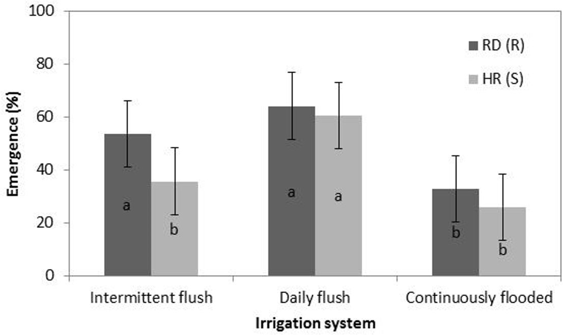
Figure 2. Emergence of RD(R) and HR(S) populations of late watergrass across intermittent flush, daily flush, and continuously flooded irrigation systems. Since there were no differences between populations at the different depths, data were averaged across four planting depths (0.5, 2, 4, and 6 cm). Bars are ± 1 SE. Different letters indicate significant differences between combinations of population and seed depth using Tukey’s HSD (α = 0.05).
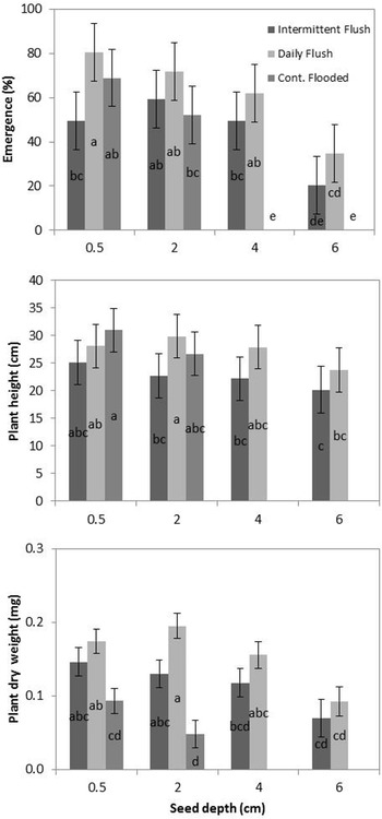
When comparing the average of the two populations, there was variation between treatments, with significantly less emergence occurring in the continuously flooded treatment compared to the intermittent flush and daily flush treatments (Figure 3), although differences were not significant between populations. This is consistent with field data with watergrass species, where shifting irrigation to flooding can be used to suppress watergrass populations (Brim-DeForest et al. Reference Brim-DeForest, Al-Khatib, Linquist and Fischer2017; Pittelkow et al. Reference Pittelkow, Fischer, Moechnig, Hill, Koffler, Mutters, Greer, Cho, van Kessel and Linquist2012). It is also consistent with the emergence data reported by Boddy et al. (Reference Boddy, Bradford and Fischer2012a), where both flooding and intermittent irrigation reduced emergence of both HR and RD populations.
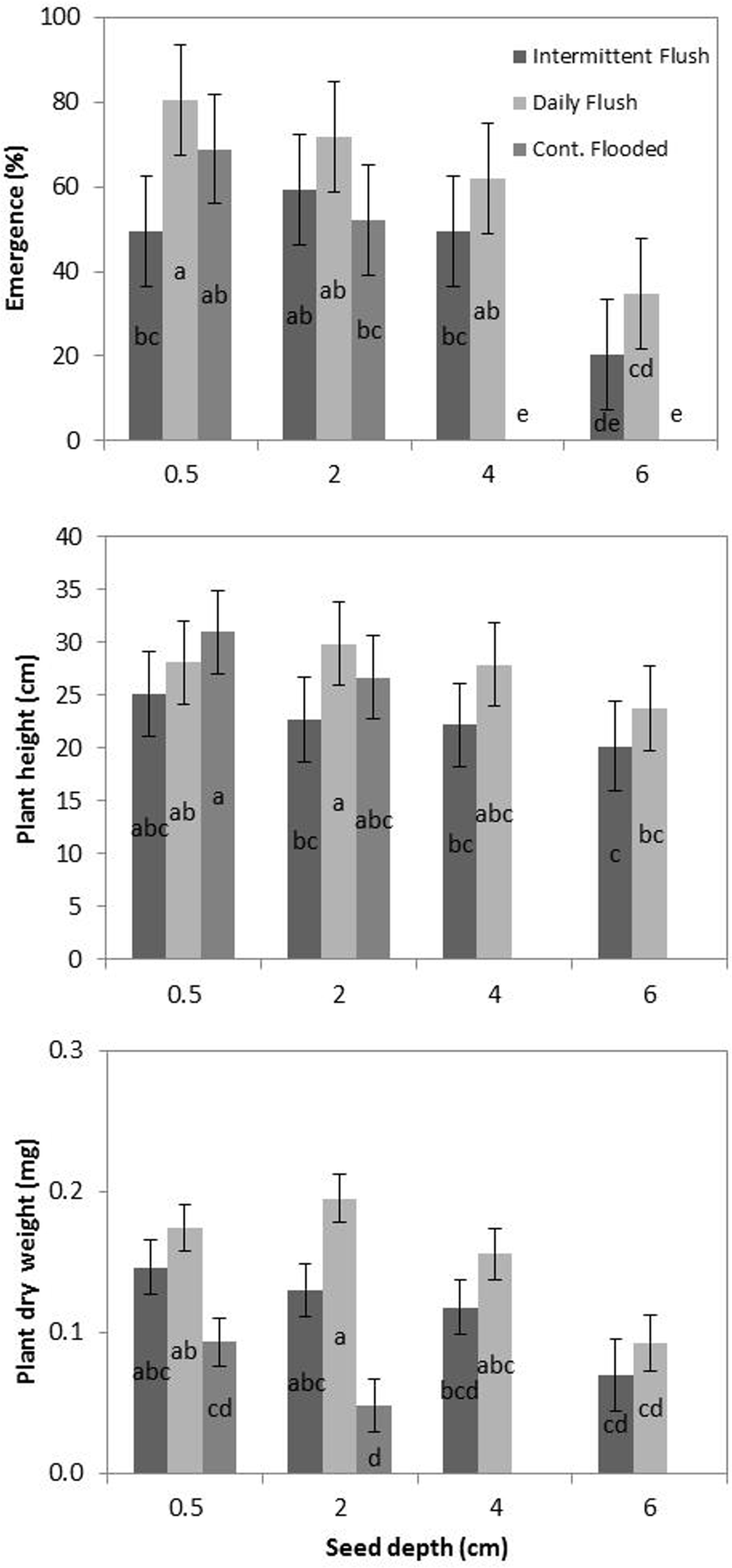
Figure 3. Emergence (top), plant height (middle), and plant dry weight (bottom) of two late watergrass populations, HR(S) and RD(R), across intermittent flush, daily flush, and continuously flooded irrigation systems. Data from the two populations were averaged across four seed depths (0.5, 2, 4, and 6 cm). Bars are ± 1 SE. Different letters indicate significant differences between combinations of seed depth × irrigation using Tukey’s HSD (α = 0.05).
Both RD and HR populations emerged from all depths (0.5 to 6 cm) in the daily flush and intermittent flush treatments; however, at 6 cm, emergence was significantly less than at 0.5, 2, and 4 cm (Figure 3). It is possible that emergence could occur at depths greater than 6 cm in these irrigation systems, and further studies should investigate the effect of deeper burial on emergence. In saturated soil, barnyardgrass [Echinochloa crus-galli (L.) Beauv.] emergence was inhibited by 50% at a depth of 5 cm. Seeds did not emerge at depths greater than 8 cm, and at 8 cm, emergence rates were only 5% to 10% (Benvenuti et al. Reference Benvenuti, MacChia and Miele2001). The intermittent flush treatment shows decreased emergence from the 0.5-cm depth in comparison to the daily flush treatment, which is similar to other studies that show decreased emergence from shallow depths in water-stressed environments (Boyd and Van Acker Reference Boyd and Van Acker2003). In the continuously flooded treatment, both populations emerged only from the 0.5- and 2-cm depths (Figure 3). This is likely due to the effects of anoxia, which may have inhibited the production of that roots can only be produced once the shoot reaches the water surface and accesses oxygen (Kennedy et al. Reference Kennedy, Barrett, Vander Zee and Rumpho1980).
There were no significant differences between RD and HR final plant dry biomass or height (data not shown). In the intermittent flush treatment, however, RD plants had slightly greater biomass, on average, than HR plants, although the difference was not significant (data not shown). Averages of both populations indicate that plants emerging from deeper depths (6 cm) had significantly smaller final heights and dry weights (Figure 3). This is consistent with other experiments on annual weeds, indicating that plants emerging from deeper burial depths have decreased height and biomass (Tang et al. Reference Tang, Busso, Jiang, Wang, Wu, Musa, Miao and Miao2016). While plants in the intermittent flush treatments were shorter and had less dry biomass than plants in the daily flush treatments, the differences were not significant. Although final height was similar, plants in the continuously flooded treatments had significantly smaller dry weight than plants in the daily flush and intermittent flush treatments. This is consistent with the results in the study by Fox et al. (Reference Fox, Kennedy and Rumpho1994) who found that early growth of late watergrass under anoxia reduced shoot weight by 75% in comparison to plants grown under aerobic conditions.
Early Growth Model
In the continuously flooded treatment, the RD population has a greater predicted growth rate (k) and a shorter predicted time to reach maximum RGR (t m ) than the HR population. It also has a shorter predicted maximum height (h max ). This is consistent across all experiments and seed depths (Table 1). In the daily flush treatment, the RD has a greater predicted growth rate (k) and a shorter predicted time to reach maximum RGR in nine of the 11 predicted curves (over the three experiments and four depths). It has a shorter maximum predicted height (h max ) in eight of the 11 predicted curves. This is consistent with the results in the study by Boddy et al. (Reference Boddy, Streibig, Yamasue and Fischer2012b), which found that resistant late watergrass plants reached maturity more quickly than the susceptible plants. In that study, plants were initially grown under saturated soil conditions, and then were flooded 1 wk after planting. In contrast to the continuously flooded and daily flush treatments, the HR population in the intermittent flush treatment had a greater predicted growth rate (k) and reached maximum RGR (t m ) more quickly than the RD population in seven out of the nine predicted curves. This may indicate that the RD population has a competitive advantage over the HR population in the intermittent flush treatment. Since the RD plants also showed greater emergence under the intermittent flush treatment, this may indicate tolerance of water stress in resistant populations; however, this remains to be further investigated. Because the resistant plants produced fewer seeds than the susceptible plants in the Boddy et al. (Reference Boddy, Bradford and Fischer2012a) study under saturated and flooded conditions, it may be that resistant plants under the intermittent flush treatment may produce more seeds in comparison to the susceptible plants. Since this could potentially affect the proportion of resistant versus susceptible seed in the seedbank, it warrants further investigation. Furthermore, due to the genetic similarity of resistant populations (Tsuji et al. Reference Tsuji, Fischer, Yoshino, Roel, Hill and Yamasue2003), it is likely that all R populations may exhibit tolerance of water stress. Due to current drought conditions in California (Jones Reference Jones2015), this may have implications for irrigation management in fields with resistant populations.
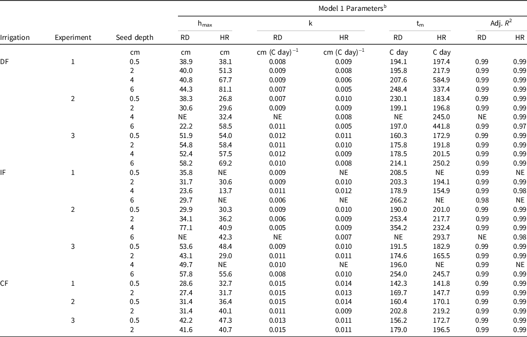
a Abbreviations: CF, continuously flooded; DF, daily flush; HR, multiple herbicide–susceptible; IF, intermittent flush; NE, not estimable; RD, multiple herbicide–resistant; RGR, relative growth rate).
b Model: h = hmax*exp(−exp(−k(t − tm))) see Gompertz (Reference Gompertz1825; where hmax = maximum predicted height, k = maximum RGR at the inflection point, and tm = time of maximum RGR.
c Models were calibrated using data from two experiments at ambient light and temperature with start dates of May 22 (1) and June 8 (2), 2013, and one greenhouse experiment (3), with a start date of September 25, 2013.
There were no differences between populations (RD and HR) in timing of predicted emergence to the 1-leaf stage (Table 2). Predicted 1-leaf stage was earliest for populations emerging from the daily flush and continuously flooded treatments, although the only significant differences were among the plants emerging from the 6-cm depth in the daily flush and intermittent flush treatments, in comparison to the plants emerging from all other depths. For the predicted 5-leaf stage, only plants emerging from the 0.5-cm and 2-cm depths were compared, since plants emerging from deeper depths did not reach the 5-leaf stage by the biomass harvest. There were no significant differences between populations (RD and HR) for the predicted timing of the 5-leaf stage. There were differences between the treatments, although they were not significant. Plants in the daily flush were predicted to reach the 1-leaf and 5-leaf stage the earliest, whereas both the intermittent flush and continuously flooded plants were slightly delayed in comparison. The delayed development is similar to the delay caused by drought stress in other plants. For example, sorghum had a decreased rate of leaf appearance when exposed to water limited conditions [Sorghum bicolor (L.) Moench; (Craufurd et al. Reference Craufurd, Flower and Peacock1993]. Likewise, prolonged flooding is known to cause reductions in dry weight and growth rate (Yu et al. Reference Yu, Stolzy and Letey1969).
Table 2. Differences in predicted 2-cm height (1-leaf stage) and 5-leaf stage values for plants emerging from the 0.5- to 6-cm depth using Equation 1. d
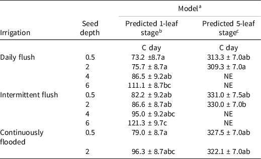
a Model: h = hmax*exp(−exp(-k(t-tm) see Gompertz (Reference Gompertz1825).
b Values (mean ± SE) followed by different letters are significantly different (P < 0.05) over all treatments and depths at each leaf stage.
c Only estimable for plants emerging from the 0.5-cm and 2-cm depths. Plants emerging from 4-cm and m depth did not reach the 5-leaf stage.
d Abbreviation: NE, not estimable.
Model Validation
The field validation of the model for HR(S) indicates good overall fit of the model in predicting late watergrass emergence (Table 3). Over both years and irrigation treatments, the fit is best in the continuously flooded treatment (average AIC = 199.05) compared to the intermittent flush treatments (average AIC = 208.6).
Table 3. Model fit for field validation of growth of herbicide-susceptible late watergrass to 2 cm (approximately the 1-leaf stage). a
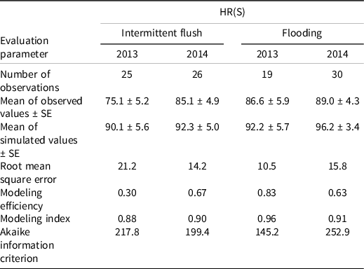
a Validation took place in intermittent flush and continuously flooded irrigation systems in 2013 and 2014.
The emergence pattern is similar in the continuous flood over the 2 yr (Figure 4). In the intermittent flush treatment there is synchrony over the 2 yr in the first emergence flush (up to approximately 60% emergence), but the difference in the emergence pattern between the 2 yr grows increasingly disparate later in the season. This is likely due to differences in soil moisture content between the two seasons after the first application of water on the field. The shape of the pattern of emergence in both treatments and years suggests that late watergrass emergence may follow a biphasic emergence pattern. This biphasic pattern is also found in the California rice agroecosystem in another weed species, smallflower umbrella sedge (Cyperus difformis L.; Brim-DeForest et al. Reference Brim-DeForest, Al-Khatib, Linquist and Fischer2017). A biphasic emergence pattern could be due to the presence of two distinct populations in the same field with different requirements for germination and dormancy (Schutte et al. Reference Schutte, Regnier, Harrison, Schmoll, Spokas and Forcella2008). It could also be due to differences in dormancy and germination requirements for different fractions of the same population (Baskin and Baskin, Reference Baskin and Baskin2001; Schutte et al. Reference Schutte, Regnier, Harrison, Schmoll, Spokas and Forcella2008).
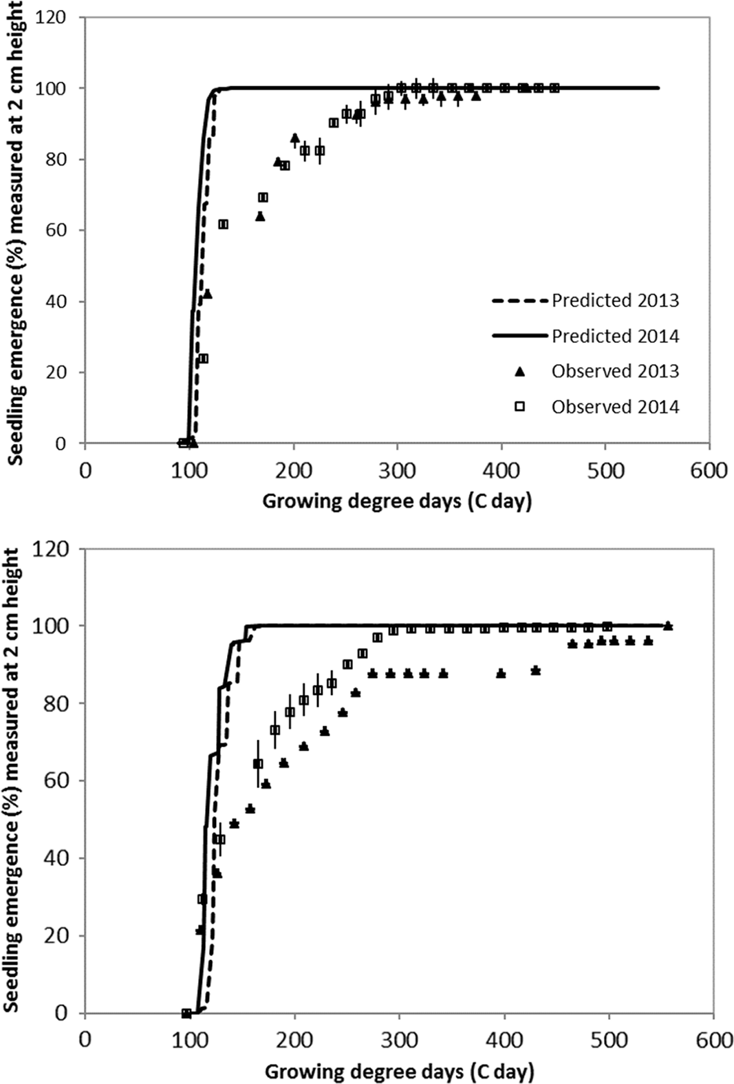
Figure 4. Validation of late watergrass emergence to 2 cm (approximately 1-leaf stage) in late watergrass under continuously flooded (top) and intermittent flush (bottom) irrigation systems. Counts were performed at the California Rice Experiment Station in Biggs, CA, in 2013 and 2014. Bars are ± 1 SE.
Late watergrass is well adapted to the rice-growing environment, and its ability to germinate and emerge under both water-stressed and anaerobic conditions further illustrates the difficulty in its management. However, its emergence is suppressed by deep burial, which suggests that no-tillage or minimum tillage may be effective in reducing emergence. This was confirmed in the field by Pittelkow et al. (Reference Pittelkow, Fischer, Moechnig, Hill, Koffler, Mutters, Greer, Cho, van Kessel and Linquist2012), who found that using reduced tillage systems significantly decreased late watergrass biomass at harvest in a continuously flooded system over a 3-yr period. The reduction was not observed in the dry-seeded system, possibly because plants were emerging from deeper in the soil. Furthermore, knowing that resistant populations may have an advantage over susceptible populations in water-stressed environments may have impacts in California because the drought has increased concerns about water management in rice, and may increase the number of farmers using dry-seeding instead of the traditionally flooded system. Predicting the first flush of late watergrass emergence could assist farmers using the stale-seedbed technique (as described by Pittelkow et al. Reference Pittelkow, Fischer, Moechnig, Hill, Koffler, Mutters, Greer, Cho, van Kessel and Linquist2012), and the model from the current study fits the first emergence flush well. However, focusing on control of the first flush may select for the later emerging weed population, so better prediction of the second emergence phase should be emphasized in future studies. Although modeling emergence of late watergrass is clearly possible, further validation in the field and the ability to model the second phase of the biphasic emergence curve is necessary before the model can be useful to farmers.
Acknowledgments
The study was funded by the California Rice Research Board. The California Rice Experiment Station and Dr. Kent McKenzie provided equipment and the experimental site. Thank you to L. Boddy and K.J. Bradford for development of the PBTM model and guidance on the experimental design for this study. The University of California-Davis Plant Sciences Department provided a graduate student assistantship to W.B. Brim-DeForest. No conflicts of interest have been declared.


 Open access