


Individuals with the poorest standard of living experience the highest rates of physical and psychiatric morbidity (Reference Blazer, Kessler and McGonagleBlazer et al, 1994; Reference Meltzer, Gill and PetticrewMeltzer et al, 1995), independent of occupational social class (Reference Davey Smith, Bartley and BlaneDavey Smith et al, 1990; Weich & Lewis, Reference Weich and Lewis1998a ,Reference Weich and Lewis b ). What is not yet known is whether health is affected by where people live. Income inequality, a population characteristic, is associated with higher mortality (Reference Kaplan, Pamuk and LynchKaplan et al, 1996; Reference Kennedy, Kawachi and Prothrow-SmithKennedy et al, 1996; Reference Fiscella and FranksFiscella & Franks, 1997; Reference WilkinsonWilkinson, 1999) and worse self-rated health (Reference Kennedy, Kawachi and GlassKennedy et al, 1998). Although Wilkinson (Reference Wilkinson1992) suggested that the effects of income inequality may be mediated by adverse psychosocial health, there have been no studies of income inequality and psychiatric morbidity. Our aims were to describe the relationships between income level, income inequality and the prevalence of the common mental disorders in Britain; and to test the hypothesis that individuals in regions of Britain with the highest income inequality have a higher prevalence of the common mental disorders, after adjusting for individual income.
METHODS
Participants
Data were gathered as part of the first wave of the British Household Panel Survey (BHPS), in autumn 1991 (Reference TaylorTaylor, 1995; Reference Weich and LewisWeich & Lewis, 1998b ). The BHPS is an annual survey of a representative sample of individuals in private households in England, Wales and Scotland. Households were selected for the BHPS using a two-stage, implicitly stratified clustered probability design, with postcode sectors as primary sampling units (Reference TaylorTaylor, 1995). The population of postcode sectors was first ordered into 18 regions (16 standard regions in England, distinguishing former Metropolitan Counties and Inner and Outer London, plus Wales and Scotland - see Table 1), resulting in a sample broadly representative of regional populations. Interviews were conducted with all members of selected households aged 16 and over. Individual BHPS participants aged 16-75 who completed the General Health Questionnaire (GHQ; Reference Goldberg and WilliamsGoldberg & Williams, 1988) were included in this analysis.
Table 1 Number of participants, prevalence of common mental disorders (% cmd), median net current equivalised weekly income (to the nearest £) and regional Gini coefficients, in descending order
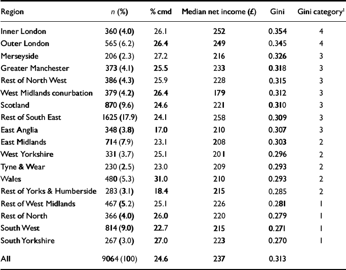
| Region | n (%) | % cmd | Median net income (£) | Gini | Gini category1 |
|---|---|---|---|---|---|
| Inner London | 360 (4.0) | 26.1 | 252 | 0.354 | 4 |
| Outer London | 565 (6.2) | 26.4 | 249 | 0.345 | 4 |
| Merseyside | 206 (2.3) | 27.2 | 216 | 0.326 | 3 |
| Greater Manchester | 373 (4.1) | 25.5 | 233 | 0.318 | 3 |
| Rest of North West | 386 (4.3) | 25.9 | 228 | 0.315 | 3 |
| West Midlands conurbation | 379 (4.2) | 26.4 | 179 | 0.312 | 3 |
| Scotland | 870 (9.6) | 24.6 | 221 | 0.310 | 3 |
| Rest of South East | 1625 (17.9) | 24.1 | 258 | 0.309 | 3 |
| East Anglia | 348 (3.8) | 17.0 | 210 | 0.307 | 3 |
| East Midlands | 714 (7.9) | 23.1 | 208 | 0.303 | 2 |
| West Yorkshire | 331 (3.7) | 25.1 | 201 | 0.296 | 2 |
| Tyne & Wear | 230 (2.5) | 23.0 | 209 | 0.293 | 2 |
| Wales | 480 (5.3) | 31.0 | 210 | 0.293 | 2 |
| Rest of Yorks & Humberside | 283 (3.1) | 18.4 | 215 | 0.285 | 2 |
| Rest of West Midlands | 467 (5.2) | 25.1 | 226 | 0.281 | 1 |
| Rest of North | 366 (4.0) | 26.0 | 220 | 0.279 | 1 |
| South West | 814 (9.0) | 22.7 | 215 | 0.271 | 1 |
| South Yorkshire | 267 (3.0) | 27.0 | 223 | 0.270 | 1 |
| All | 9064 (100) | 24.6 | 237 | 0.313 |
Table 2 Percentage of participants who were cases of the common mental disorders, and adjusted odds ratio (95% CI)1 for prevalence of the common mental disorders by category of Gini coefficient calculated using net current income, stratified by household (net) income rank (fifths within region). The odds of being a case for each group were compared with those for participants in the top income fifth in regions with the lowest Gini coefficients (> 1 standard deviation below the mean for the entire British Household Panel Survey sample at wave 1)
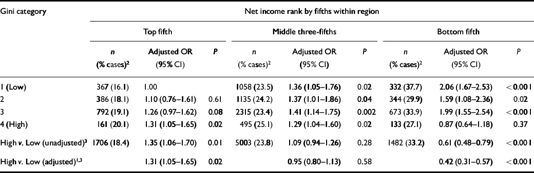
| Gini category | Net income rank by fifths within region | ||||||||
|---|---|---|---|---|---|---|---|---|---|
| Top fifth | Middle three-fifths | Bottom fifth | |||||||
| n (% cases)2 | Adjusted OR (95% CI) | P | n (% cases)2 | Adjusted OR (95% CI) | P | n (% cases)2 | Adjusted OR (95% CI) | P | |
| 1 (Low) | 367 (16.1) | 1.00 | 1058 (23.5) | 1.36 (1.05-1.76) | 0.02 | 332 (37.7) | 2.06 (1.67-2.53) | < 0.001 | |
| 2 | 386 (18.1) | 1.10 (0.76-1.61) | 0.61 | 1135 (24.2) | 1.37 (1.01-1.86) | 0.04 | 344 (29.9) | 1.59 (1.08-2.36) | 0.02 |
| 3 | 792 (19.1) | 1.26 (0.97-1.62) | 0.08 | 2315 (23.4) | 1.41 (1.14-1.75) | 0.002 | 673 (33.9) | 1.99 (1.55-2.54) | < 0.001 |
| 4 (High) | 161 (20.1) | 1.31 (1.05-1.65) | 0.02 | 495 (25.1) | 1.29 (1.04-1.60) | 0.02 | 133 (27.1) | 0.87 (0.64-1.18) | 0.37 |
| High v. Low (unadjusted)3 | 1706 (18.4) | 1.35 (1.06-1.70) | 0.01 | 5003 (23.8) | 1.09 (0.94-1.26) | 0.28 | 1482 (33.2) | 0.61 (0.48-0.79) | < 0.001 |
| High v. Low (adjusted)1,3 | 1.31 (1.05-1.65) | 0.02 | 0.95 (0.80-1.13) | 0.58 | 0.42 (0.31-0.57) | < 0.001 | |||
Assessment of common mental disorders
Common mental disorders were assessed using the self-administered 12-item GHQ (Reference Goldberg and WilliamsGoldberg & Williams, 1988). The GHQ is a measure of recent changes in one's usual mental state, and although some individuals with chronic symptoms of anxiety and depression may be misclassified, the false negative rate in a previous community study was low (7%) (Reference Goldberg and WilliamsGoldberg & Williams, 1988). We followed previous studies in treating the common mental disorders as a single dimension (Reference Goldberg and HuxleyGoldberg & Huxley, 1992; Reference Lewis and BoothLewis & Booth, 1992; Reference Stansfeld and MarmotStansfeld & Marmot, 1992). Each item on the GHQ was scored as present or absent, and those scoring 3 or more (out of 12) were classified as cases (Reference BanksBanks, 1983; Reference Goldberg and WilliamsGoldberg & Williams, 1988; Weich & Lewis, Reference Weich and Lewis1998a ,Reference Weich and Lewis b ). Although results are presented here for ‘cases’ of common mental disorders, there was no reason to expect that using GHQ scores as a continuous variable would lead to different results (Reference Anderson, Huppert and RoseAnderson et al, 1993; Reference Weich and LewisWeich & Lewis, 1998a ).
Measures of income
Gross income data, expressed as pounds sterling per week, were collected by source for each BHPS participant, and aggregated for households. Gross income data include earnings from employment, self-employment, savings, investments and private and occupational pensions, and from cash social security and social assistance benefits. Net household income is equal to gross household income less income tax payments, National Insurance contributions and local taxes. These data were constructed for all persons in the survey by means of a simulation model of the tax system (Reference Jarvis and JenkinsJarvis & Jenkins, 1995). BHPS net income data were validated against contemporaneous data from the Family Expenditure Survey (FES), used by the Department of Social Security to compile official income distribution figures for the UK (Reference Jarvis and JenkinsJarvis & Jenkins, 1995).
Wherever possible, BHPS interviewers sought documentary confirmation of income data. Missing gross income data were imputed by the BHPS investigators (Reference TaylorTaylor, 1995; Reference Weich and LewisWeich & Lewis, 1998a ). These values were used to reduce potential bias arising from the exclusion of missing data. Net income data could not be estimated for the small number of households in which one or more adults refused to be interviewed, because imputed values for missing income components are not available.
All income data were adjusted using the McClements (before housing costs) Equivalence Scale (Reference TaylorTaylor, 1995), to take account of differences in household size and composition. In keeping with standard practice (Reference Jarvis and JenkinsJarvis & Jenkins, 1995), each individual was attributed with the equivalent (net or gross) income of the household to which he or she belonged.
Participants were classified in two ways according to their income. First, individuals were allocated to one of 11 bands, starting at <£100 per week and increasing in increments of £50 per week. Second, individuals were classified by income rank, by quintile group within region (Weich & Lewis, Reference Weich and Lewis1998a ,Reference Weich and Lewis b ). At the time of writing, the exchange rate was approximately £1=0.7 euro.
Measure of income inequality, by region
Gini coefficients for each region were calculated using a program written by one of the authors (S.P.J.) (Reference JenkinsJenkins, 1999). The Gini coefficient is a measure of inequality that ranges from 0.0 when everyone has the same income (perfect equality) to 1.0 when one person has all the income (perfect inequality). We used the Gini coefficient because it is the most widely used summary measure of income inequality and has a neat relationship with the Lorenz curve for incomes. This measure also has the advantage of being relatively insensitive to the presence of outlier incomes at the top and bottom of the income distribution. Although there are many measures of income inequality, all are highly correlated with one another, and similar in their correlations with mortality (Reference Kawachi and KennedyKawachi & Kennedy, 1997). We evaluated the sensitivity of our findings to the choice of inequality measure by repeating our analyses using three other inequality indices (the mean log deviation, the Theil index and half the squared coefficient of variation). These indices are members of the generalised entropy class of inequality indices with parameters 0, 1 and 2 respectively (Reference JenkinsJenkins, 1999). These income inequality indices aggregate income differences among high, middle and poor incomes in different ways. Given that income was not normally distributed, median net income was chosen as the indicator of the central tendency of income distribution within each region.
Regional Gini coefficients were calculated for current gross and net income, using the entire BHPS wave 1 sample, and divided into four categories. Category 1 (‘low Gini coefficient’) included regions with Gini coefficients less than one standard deviation below the mean; category 2 included regions with coefficients within one standard deviation below the mean; category 3 included regions with coefficients within one standard deviation above the mean; and category 4 (‘high Gini coefficient’) included regions with coefficients in excess of one standard deviation above the mean (Table 1).
Other potential confounders
Based on previous findings (Weich & Lewis, Reference Weich and Lewis1998a ,Reference Weich and Lewis b ), age, gender, housing tenure, Registrar General's social class by head of household, marital status, education, employment, ethnicity, and the number of current physical health problems for each participant were included as potential individual-level confounders of any association between income inequality and common mental disorders.
Statistical analysis
All analyses were undertaken using Stata (Stata Corporation, 1999). Unadjusted and adjusted odds ratios with 95% confidence intervals, and likelihood ratio tests (LRTs) to assess departure from linear trends, confounding and effect modification were calculated by means of logistic regression. Since data were clustered within both households and regions, we adjusted the standard errors of regression coefficients using the Huber-White sandwich estimate of variance (Reference HuberHuber, 1981; Stata Corporation, 1999), specifying region as the highest-level cluster. This method relaxes the assumption of independence of observations within clusters. Since it is insensitive to the correlation structures within the highest-level cluster, it also corrects standard errors for any clustering of data at all nested levels below that specified.
Analyses were undertaken separately using both net and gross (individual) income level, and Gini coefficients calculated using distributions of both net and gross income. Except where findings differed, results are presented only for analyses using individual and regional indices based on net income, since these were judged a priori to be the most valid indices of individual and regional income, after allowing for the redistributive effects of taxation.
RESULTS
After excluding ‘deadwood’ addresses, 73.6% of households (n=5511) participated in the first BHPS wave, comprising 9612 individuals aged 16-75. Estimates of current gross income were available for the entire sample. Estimates of current net income were available for 4826 households (87.6%), and 8371 individuals aged 16-75. In total, 8191 participants were included in the present analyses, amounting to 85.2% of those aged 16-75 who were interviewed at wave 1 of the BHPS, or approximately 63% of the non-deadwood issued sample for this survey (assuming similarity in the age distributions of participants and non-participants). The prevalence of common mental disorders in the study sample was 24.6% (95% CI 23.7-25.5).
Income inequality by region
The median Gini coefficient by region (using net income) was 0.309 (range 0.270-0.354) (Table 1). Two regions (Inner and Outer London) were classified as ‘high Gini’ regions, and four as ‘low Gini’ regions (South Yorkshire, Southwest, Rest of North and Rest of West Midlands). Statistically significant associations were found between (higher) Gini coefficients and the proportion of participants living in rented accommodation (χ2=57.2, d.f.=3, P<0.001) and unemployed (for net income, χ2=13.0, d.f.=3, P=0.005). Regions with higher Gini coefficients had a higher proportion of residents with at least one educational qualification (for net income, χ2=36.5, d.f.=3, P<0.001), and higher median (net) regional income (Spearman's r=0.46, P<0.0001).
Individual income, median regional income and prevalence of the common mental disorders
A statistically significant association was found between the prevalence of the common mental disorders and current net income, which departed from linearity to a statistically significant degree — LRT χ2=39.0, d.f.=9, P<0.0001 (Fig. 1). A similar association was found using current gross income. There was no evidence of a statistically significant association between the prevalence of the common mental disorders and median regional net income, whether treated as a continuous or as a categorical measure.
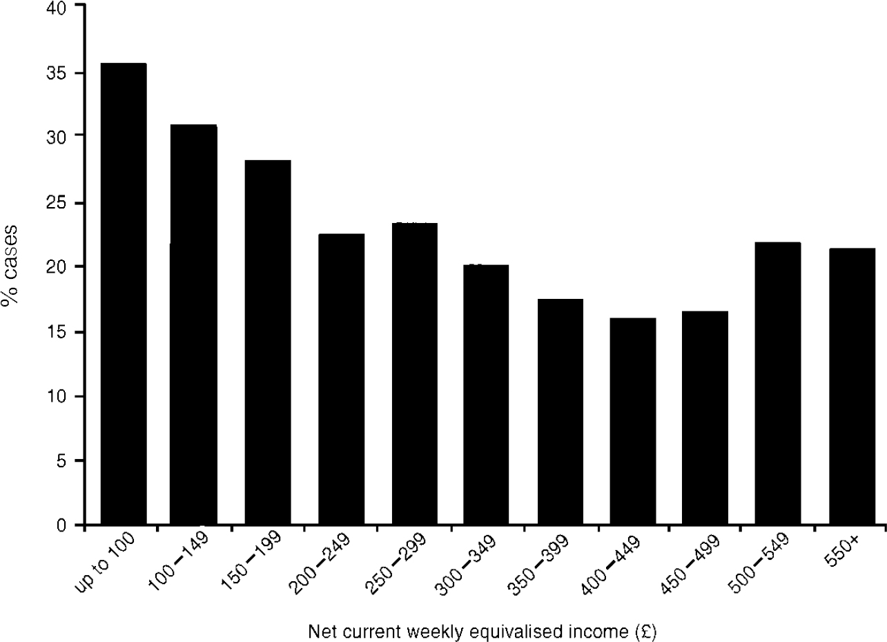
Fig. 1 Prevalence of the common mental disorders by net current weekly equivalised income.
Income inequality and prevalence of the common mental disorders
No statistically significant association was found between Gini coefficient and the common mental disorders (for Gini category 4 v. category 1, unadjusted OR=0.99, 95% CI 0.87-1.13; P=0.88). However, a statistically significant interaction was found between income level (whether absolute or rank) and regional Gini coefficients in their associations with the prevalence of the common mental disorders (LRT χ2 on removing interaction term=4.39, d.f.=1; P=0.04) (Table 2). Odds ratios for the association between Gini coefficient category and the prevalence of the common mental disorders increased with individual income, irrespective of how the latter was measured. Among those with the highest incomes, the prevalence of the common mental disorders was significantly higher among individuals living in ‘high Gini’ than in ‘low Gini’ regions, after adjusting for potential individual-level confounders. Among those with the lowest incomes the reverse was true, such that the prevalence of these disorders was lower in ‘high Gini’ than ‘low Gini’ regions, to a statistically significant degree. These findings were not altered substantially on adjusting for other potential confounders (Table 2). Finally, sensitivity analyses indicated that our findings were not altered by the choice of inequality measure (see Methods).
DISCUSSION
Main findings
The two most notable findings were the non-linear association between income and the common mental disorders, and the statistically significant interaction between income inequality and income level in their associations with the prevalence of these disorders. The use of net rather than gross income to calculate income inequality and to quantify individual financial resources did not alter these findings.
The interaction between income level and income inequality makes it difficult to summarise the relative importance of each for the prevalence of the common mental disorders. In all but those regions with the highest income inequality (the two London regions), low income level was associated with an increase in the risk of being a case of the common mental disorders by between 60% and 110%. Among those with the highest income levels, the increased risk of the common mental disorders among those living in regions with the highest income inequality, compared with their counterparts in the most egalitarian regions, was about 35%.
Methodological strengths and weaknesses
This is the first study to consider the effects of income inequality on rates of psychiatric morbidity, and moreover we are not aware of any other studies that have considered the effects of income inequality on health within Britain. This is also one of the first studies to estimate income inequality after the redistributive effects of taxation, using net income data. Finally, the present study was one of only a handful to control for household income, using the individual as the unit of analysis (Reference Fiscella and FranksFiscella & Franks, 1997; Reference Kennedy, Kawachi and GlassKennedy et al, 1998).
These findings are based on a cross-sectional survey, which precludes causal inference. Bias in the recall of income was unlikely, given reliance on documentation wherever possible. Selective migration of wealthy cases of the common mental disorders to regions with the greatest income inequality seems improbable. Although the common mental disorders may contribute to income inequality through economic inactivity or unemployment, the effect of this was likely to have been small. Furthermore, the data used to calculate Gini coefficients were drawn from the entire BHPS wave 1 sample, and not just participants included in our analyses. Regional differences in the extent and distribution of undeclared income may have resulted in biased estimates of income inequality, although little is known about this subject. We are not aware of any evidence that undeclared income varies by region or income level, and there is no reason to suspect that the BHPS is any worse (or better) than other national household surveys at measuring income (Reference Jarvis and JenkinsJarvis & Jenkins, 1995). Nonresponse bias cannot be dismissed, since our sample was about 65% of the target sample. However, for this to have affected the association between the common mental disorders and income inequality, participation in the first wave of the BHPS would have to have been associated with GHQ score, region of residence and household income.
The GHQ, rather than a standardised clinical interview, was used to assess the common mental disorders. Despite the high sensitivity of the GHQ (Reference Goldberg and WilliamsGoldberg & Williams, 1988), the gradient in common mental disorders by individual income may have been underestimated as a result of misclassification of individuals with chronic symptoms of anxiety and depression, and any tendency for those of low socio-economic status to underreport psychiatric symptoms. These were unlikely to have altered our main findings (Reference Goldberg and WilliamsGoldberg & Williams, 1988; Reference Newman, Bland and OrnNewman et al, 1988).
Among the most salient features of any study of this nature are the size of the area over which income data are aggregated (Reference Kennedy, Kawachi and GlassKennedy et al, 1998) and the geographical and socio-economic variation across these clusters. Previous studies that have reported statistically significant associations between income inequality and different health outcomes have used data aggregated at the level of countries or US states. While lack of variation in income inequality between UK regions might be a problem, it may be that these regions were too small to permit income inequality to exert an independent effect on health, after adjusting for individual income. Wilkinson (Reference Wilkinson2000) suggests that people in deprived neighbourhoods do not have bad health because of inequalities within neighbourhoods, but because these neighbourhoods are deprived in relation to the wider society. He argues that, in moving from larger to smaller areas, median income becomes a more important predictor, and income inequality a weaker predictor, of mortality. The absence of an association between regional median income and the prevalence of the common mental disorders may perhaps be viewed as further evidence against an area-level effect on individual mental health (Reference WilkinsonWilkinson, 2000). Our analyses were also conducted at the level of region for pragmatic reasons, in keeping with the structure and organisation of the BHPS data-set. The BHPS data-set contains insufficient observations per district to derive sufficiently reliable estimates of income inequality at levels below regions. While acknowledging the limitations that this imposed on our study, and the somewhat artificial nature of the administrative boundaries between regions, we would argue that this is both a theoretically and empirically valid level at which to study the effects of income inequality in Britain.
The range of Gini coefficients in this study was quite a large spread for this index. It was at least as large as the change in the overall Gini coefficient for the United Kingdom from the mid-1970s to the 1990s — a change which is considered by most to have been very large (Reference Lynch, Davey Smith and KaplanLynch et al, 2000). The range of regional Gini scores in the present study was also similar to that observed across US states in the study by Kennedy et al (Reference Kennedy, Kawachi and Glass1998).
Effects of London regions
Of most concern is the possibility of confounding by other contextual characteristics of the regions, particularly since the two regions with the highest income inequality were Inner and Outer London. The increased prevalence of the common mental disorders among those with the highest incomes in these regions, and the reduced prevalence among those with the lowest incomes, may be due to characteristics of the regions other than income inequality. For example, the stresses experienced by those with the highest incomes may be greater in London than elsewhere because of transport difficulties or higher crime rates. Similarly, the difficulties of life on a low income may be eased in London by greater access to social housing, public transport and other amenities.
Income inequality, higher individual income and worse mental health
Because the association between individual income level and mortality is non-linear (Reference WilkinsonWilkinson, 1992), it has been argued that the association between mortality and income inequality in ecological studies may have arisen because areas of high inequality have more poor people (Reference GravelleGravelle, 1998). Two previous studies controlled for household income but produced contradictory results (Reference Fiscella and FranksFiscella & Franks, 1997; Reference Kennedy, Kawachi and GlassKennedy et al, 1998). The latter found that the association between income inequality (using the Gini index) and worse self-rated health increased with lower individual income, and was attenuated by other individual socio-economic characteristics.
By contrast, we found a modest independent association between regional income inequality and the common mental disorders among those with the highest incomes within their region of residence. This finding was not confounded by individual income or other socio-economic circumstances. Our findings suggest that the most affluent individuals living in areas of highest income inequality experience worse psychosocial health, and hence lower quality of life, than their counterparts in regions where income is distributed more equally. Although not a test of Wilkinson's hypothesis (Reference WilkinsonWilkinson, 1992) our findings indicate that income inequality may have important public health consequences beyond raised mortality rates. Our findings also run counter to the notion that the most affluent benefit in a highly stratified, competitive and unequal society.
Possible explanations for study findings
There are many possible explanations for these counter-intuitive results. Although confounding by other contextual factors cannot be excluded, it is possible that those with the highest incomes in regions with higher income inequality may experience greater stresses than the most affluent elsewhere. Since a higher income is needed to get into this top income band in regions with the highest income inequality, individuals may have to work harder to maintain their social position. As well as recognising that they have ‘further to fall’ than counterparts elsewhere, guilt or unease about the relative disadvantage of others may also play a part. These intriguing hypotheses, although speculative, warrant further investigation.
Clinical Implications and Limitations
CLINICAL IMPLICATIONS
-
▪ The present study is among the first to provide empirical support for the view that the places where people live affect their mental health, independently of their individual characteristics.
-
▪ People with higher incomes who lived in regions of Britain with relatively unequal income distributions had a higher prevalence of the common mental disorders than those living in regions where income was more equally distributed. This was not the case for the least well off.
-
▪ The association between individual income and prevalence of the common mental disorders was non-linear, and followed a reverse J-shape. Interventions to alleviate the effects of poverty on the prevalence of the common mental disorders are therefore likely to be of greatest benefit if targeted at those on the lowest incomes.
LIMITATIONS
-
▪ The cross-sectional study design limits causal inference.
-
▪ The use of a self-administered measure of psychiatric morbidity means that a proportion of those identified as ‘cases’ would not have met diagnostic criteria for clinical disorders.
-
▪ The study findings may have been confounded by characteristics of the London regions other than their high income inequality.
ACKNOWLEDGEMENTS
The authors are grateful to Richard Wilkinson and Ichiro Kawachi for their comments on earlier drafts of this paper. The data used in this manuscript were made available through the ESRC Data Archive. The data were originally collected by the ESRC Research Centre on Micro-social Change at the University of Essex. Neither the original collectors of the data nor the Archive bear any responsibility for the analyses or interpretations presented here. The Institute for Social and Economic Research receives core funding from the ESRC and the University of Essex.


eLetters
No eLetters have been published for this article.