


1. Introduction
During the process of service or industrial operations, robotic arms require flexibility and safety to avoid damage to themselves or the environment. In biology, due to the complexity of bones, the redundancy of muscle distribution, the nonlinearity of muscles, and the uniqueness of muscle control of neural mechanisms, the human arm can dexterously, flexibly, and safely complete complex manipulation tasks [Reference Mizuuchi, Nakanishi, Sodeyama, Namiki, Nishino, Muramatsu, Urata, Hongo, Yoshikai and Inaba1–Reference Li, Li and Kan3]. The operation of musculoskeletal robots with humanoid structures can be considered to avoid danger to humans and the environment, possibly because they have redundant muscles that provide robustness and flexibility during variable stiffness control [Reference Kawamura, Ookubo, Asano, Kozuki, Okada and Inaba4–Reference Kawaharazuka, Makino, Kawamura, Asano, Okada and Inaba6]. In recent years, the structural design, simulation modeling, and muscle control of anthropomorphic robots have been widely studied by scholars [Reference Mizuuchi, Nakanishi, Sodeyama, Namiki, Nishino, Muramatsu, Urata, Hongo, Yoshikai and Inaba1, Reference Jantsch, Wittmeier, Dalamagkidis, Panos, Volkart and Knoll7, Reference Asano, Okada and Inaba8]. In terms of structural design, most scholars install artificial muscle units on the arm to provide tension for the elbow joint, forearm joint, or finger, which increases the arm’s weight and makes it difficult to control [Reference Mizuuchi, Nakanishi, Sodeyama, Namiki, Nishino, Muramatsu, Urata, Hongo, Yoshikai and Inaba1, Reference Jantsch, Wittmeier, Dalamagkidis, Panos, Volkart and Knoll7, Reference Asano, Okada and Inaba8]. Aiming at the difficulty of modeling the anthropomorphic musculoskeletal hardware platform, our team has built a complete hardware platform of a lightweight musculoskeletal arm, as shown in Fig. 1. In order to make the system lightweight, the drive unit is arranged in the chest cavity and drives the arm via a cable. However, with the design of the distal arrangement of the artificial muscle unit, the problem of friction in the process of transmitting muscle tension by the cable is more serious. This system makes the general adaptive control method unable to effectively eliminate the friction of the cable. It mainly shows the friction between the cable and the inner wall of the pipeline and the friction between the cable and the pulley or other contact parts.

Figure 1. Musculoskeletal system.
The cable-driven method is widely used in industrial places such as cranes and elevators [Reference Wei, Qiu and Sheng9, Reference Wittmeier, Alessandro, Bascarevic, Dalamagkidis, Devereux, Diamond, Jäntsch, Jovanovic, Knight, Marques, Milosavljevic, Mitra, Svetozarevic, Potkonjak, Pfeifer, Knoll and Holland10], as well as exoskeletons, surgical robots, dexterous hands, and musculoskeletal system (MS) robots. Due to the advantages of light weight, flexible transmission, and long transmission distance [Reference Wei, Qiu and Sheng9–Reference Kim, Jung, Jeong, Park, Jung, Cheong, Choi, Do and Park11], the cable-drive system has special applications in the field of machinery. Cable drives also have shortcomings such as easy tensile deformation and significant contact friction, which are affected by factors such as materials, preload, lubrication conditions, and support and restraint structure design [Reference Wei, Qiu and Sheng9–Reference Kim, Jung, Jeong, Park, Jung, Cheong, Choi, Do and Park11]. The problems existing in the application of cable drive are studied.
On the other hand, the skeletal structure can be considered as consisting of connecting rods connected sequentially through rotating joints. Several scholars have studied the friction problem of ordinary robots [Reference Lischinsky, Canudas-de-Wit and Morel12–Reference Kawaharazuka, Kawamura, Makino, Asano, Okada and Inaba16]. Based on the LuGre dynamic model, Lischinsky developed a friction model for a hydraulically driven manipulator [Reference Lischinsky, Canudas-de-Wit and Morel12]. B. Jin determined the friction parameters of a harmonic reducer with reference to the Coulomb + Viscosity + Stribeck model [Reference Jin, Sun, Zhang, Ding, Lin, Deng, Zhu and Sun13]. In addition, some scholars such as Katz pointed out that friction is influenced by motor torque [Reference Katz, Carlo and Kim14]. When the robot arm cannot move to the desired position due to the wrong model, the cable appears overloaded/slack and even damages the robot [Reference Kawaharazuka, Kawamura, Makino, Asano, Okada and Inaba16].
The installation structure at the far end of the artificial muscle unit in the cable-driven manner involved in this paper brings about a significant problem of the frictional force of the cable [Reference Yuan, Wu, Wang and Qiao17]. Muscle antagonism distribution structures are prone to muscle hyper-relaxation/tension as shown in Fig. 2. When the cable transmits muscle force, the tube will deform, and the contact surface with the tube is uncertain and random.

Figure 2. The situations of the cable.
Furthermore, the control of robotic manipulators with the environment is still affected by its unknown dynamics, inner coupling effects, and unknown disturbance [Reference Zhao, Liu, Li, Su and Feng15]. Addressing on such difficulty, the adaptive neural networks have strong ability to model the unknown system dynamics [Reference Zhao, Liu, Li, Su and Feng15]. In order to improve adaptability to meet high-performance operation requirements, Su et al. introduced two multi-layer neural network approaches to enhance the sensing accuracy of the end-of-manipulator tool [Reference Su, Qi, Hu, Sandoval, Zhang, Schmirander, Chen, Aliverti, Knoll, Ferrigno and De Momi18]. In view of the above problems, this paper proposes the following solutions:
-
Aiming at the friction generated by the contact between the cable and the restraining structure/tube in the process of muscle force transmission, a friction feedforward compensation method based on neural network fitting is proposed.
-
Aiming at the problem that the cable can only transmit tension and antagonize the excessive relaxation/tension of the cable between artificial muscles, a cable relaxation model is proposed, and the mapping relationship between the joint space and the muscle space is given.
-
The model of the MS is established on the hardware platform, and the trajectory tracking control verification is completed.
2. Method
In the MS as shown in Fig. 1, the friction is mainly divided into the tubing friction generated by the cable through the casing and the friction generated by the linkage joint. In addition, there will be some slack phenomenon when the robotic arm stops due to the underestimation of system dynamics, as shown in Fig. 2. The blue line indicates a slack cable, and the red line indicates a tensioned cable. In the case of redundant muscles working in concert to control the shoulder joint, a particular slack cable can increase the load on other cables or even cause an unstable load on the robot arm. The friction of a cable can be described by its state. The speed of the cable can be approximated by the product of the motor speed and the radius of the winch. A significant error between the increment of the cable length and the increment of the muscle length indicates slack in the cable.
2.1. Problem formulation
For cable-driven robotic arms, the pull of the cable provides the joint wrench.
 \begin{equation} dq_{MS}\cdot \tau _{MS}=dl_{M}\cdot f_{M} \end{equation}
 \begin{equation} \tau _{\mathrm{MS}}=dl_{M}/dq_{MS}\cdot f_{M}=J_{c}\!\left(q_{MS}\right)f_{M} \end{equation}
 \begin{equation} \dot{l}_{M}=J_{c}\!\left(q_{\mathrm{MS}}\right)\dot{q}_{\mathrm{MS}} \end{equation}
 \begin{equation} \ddot{l}_{M}=\dot{J}_{c}\!\left(q_{\mathrm{MS}}\right)\dot{q}_{\mathrm{MS}}+J_{c}\!\left(q_{\mathrm{MS}}\right)\ddot{q}_{\mathrm{MS}} \end{equation}
where $l_{\mathbf{M}},\dot{l}_{M},\ddot{l}_{M}\in \mathrm{\mathbb{R}}^{m}$
are the position, velocity, and acceleration vectors of the muscle, respectively,
$l_{\mathbf{M}},\dot{l}_{M},\ddot{l}_{M}\in \mathrm{\mathbb{R}}^{m}$
are the position, velocity, and acceleration vectors of the muscle, respectively, $dq_{MS}$
is the differential of the joint state,
$dq_{MS}$
is the differential of the joint state, $dl_{M}$
is the differential of the cable displacement, and the Jacobi matrix
$dl_{M}$
is the differential of the cable displacement, and the Jacobi matrix $J_{c}(q_{\mathrm{MS}})\in \mathrm{\mathbb{R}}^{m\times n}$
relates to the muscle force vector
$J_{c}(q_{\mathrm{MS}})\in \mathrm{\mathbb{R}}^{m\times n}$
relates to the muscle force vector $f_{M}\in \mathrm{\mathbb{R}}^{m}$
and the system torque
$f_{M}\in \mathrm{\mathbb{R}}^{m}$
and the system torque $\tau _{MS}$
. The muscle force is limited by a positive feasible muscle force set
$\tau _{MS}$
. The muscle force is limited by a positive feasible muscle force set $0\leq f_{\min }\leq\, f_{{M_{i}}}\leq\, f_{\max }, \forall i\colon f_{{M_{i}}}\in\, f_{M}$
, where
$0\leq f_{\min }\leq\, f_{{M_{i}}}\leq\, f_{\max }, \forall i\colon f_{{M_{i}}}\in\, f_{M}$
, where $f_{\min }$
is the minimum force and
$f_{\min }$
is the minimum force and $f_{\max }$
is the maximum force.
$f_{\max }$
is the maximum force.
The robotic arm can be modeled as a multi-linked cable-driven robot. The following equations can describe the system dynamics of an n-DOF musculoskeletal robot with m muscles:
 \begin{equation} D_{M}\!\left(q_{MS}\right)\ddot{q}_{MS}+C\!\left(q_{MS},\dot{q}_{MS}\right)\dot{q}_{MS}+G\!\left(q_{MS}\right)=\tau _{MS}-T_{f} \end{equation}
where $q_{MS}\in \mathrm{\mathbb{R}}^{n}$
is the generalized coordinate,
$q_{MS}\in \mathrm{\mathbb{R}}^{n}$
is the generalized coordinate, $D_{M}(q_{MS})\in \mathrm{\mathbb{R}}^{n\times n}$
is the inertia matrix,
$D_{M}(q_{MS})\in \mathrm{\mathbb{R}}^{n\times n}$
is the inertia matrix, $C(q_{\mathrm{MS}},\dot{q}_{MS})\in \mathrm{\mathbb{R}}^{n}$
is the centrifugal Coriolis vector,
$C(q_{\mathrm{MS}},\dot{q}_{MS})\in \mathrm{\mathbb{R}}^{n}$
is the centrifugal Coriolis vector, $G(q_{\mathrm{MS}})\in \mathrm{\mathbb{R}}^{n}$
is the gravitational vector,
$G(q_{\mathrm{MS}})\in \mathrm{\mathbb{R}}^{n}$
is the gravitational vector, $\tau _{MS}\in \mathrm{\mathbb{R}}^{n}$
is the system wrench, and
$\tau _{MS}\in \mathrm{\mathbb{R}}^{n}$
is the system wrench, and $T_{f}\in \mathrm{\mathbb{R}}^{n}$
is the error of the wrench acting on the system. The variable
$T_{f}\in \mathrm{\mathbb{R}}^{n}$
is the error of the wrench acting on the system. The variable $T_{f}$
contains the effects of cable friction
$T_{f}$
contains the effects of cable friction $T_{p}$
, rigid friction
$T_{p}$
, rigid friction $T_{\textit{friction}}$
, and muscle antagonistic relaxation
$T_{\textit{friction}}$
, and muscle antagonistic relaxation $\tau _{r}$
on the system.
$\tau _{r}$
on the system.
The number of muscles is nine, and the number of joints is four. It indicates the degree of muscle contraction when the joint moves in a particular direction when the joint angle is $q_{MS}$
. The muscle Jacobi matrix
$q_{MS}$
. The muscle Jacobi matrix $J_{c}(q_{MS})$
is denoted as
$J_{c}(q_{MS})$
is denoted as $J_{c}(q_{MS})=dl_{M}/dq_{MS}$
. When the target joint angle is
$J_{c}(q_{MS})=dl_{M}/dq_{MS}$
. When the target joint angle is $\hat{q}_{MS}$
, and the current joint angle is
$\hat{q}_{MS}$
, and the current joint angle is $q_{MS}, J_{c}(q_{MS})\cdot (\hat{q}_{MS}-q_{MS})$
indicates whether each muscle is an agonist or an antagonist’s muscle when moving to that position. In the literature [Reference Kawaharazuka, Kawamura, Makino, Asano, Okada and Inaba16], antagonistic muscle relaxation
$q_{MS}, J_{c}(q_{MS})\cdot (\hat{q}_{MS}-q_{MS})$
indicates whether each muscle is an agonist or an antagonist’s muscle when moving to that position. In the literature [Reference Kawaharazuka, Kawamura, Makino, Asano, Okada and Inaba16], antagonistic muscle relaxation $\tau _{r}$
was expressed as:
$\tau _{r}$
was expressed as:
 \begin{align} \begin{cases} \tau _{r}=K_{s}\cdot \left(l_{M}-\hat{l}_{M}\right) & J_{c}\!\left(q_{\mathrm{MS}}\right)\cdot \frac{\hat{q}_{\mathrm{MS}}-q_{\mathrm{MS}}}{\left| \hat{q}_{\mathrm{MS}}-q_{\mathrm{MS}}\right| }\lt C_{\mathrm{MS}}\\[5pt] \tau _{r}=0 & \text{otherwise} \end{cases} \end{align}
where $hatl_{M}$
is the desired cable length,
$hatl_{M}$
is the desired cable length, $l_{M}$
is the actual cable length,
$l_{M}$
is the actual cable length, $hatq_{M}$
is the angle of the desired joint, and
$hatq_{M}$
is the angle of the desired joint, and $q_{MS}$
is the angle of the actual joint.
$q_{MS}$
is the angle of the actual joint. $C_{MS}$
is a constant.
$C_{MS}$
is a constant.
The connection between the output $(T_{\text{output}})$
and the input
$(T_{\text{output}})$
and the input $(T_{in})$
is
$(T_{in})$
is $T_{\mathrm{in}}=T_{\text{output}}/r_{\text{winch}}$
. The output of the sensor is
$T_{\mathrm{in}}=T_{\text{output}}/r_{\text{winch}}$
. The output of the sensor is $\mathrm{T}_{\mathrm{in}}=\mathrm{F}_{\text{sensor}}$
. Theoretically, the relationship between the length of the tensioned cable and the angle of the joint is
$\mathrm{T}_{\mathrm{in}}=\mathrm{F}_{\text{sensor}}$
. Theoretically, the relationship between the length of the tensioned cable and the angle of the joint is $\hat{l}_{M}={\unicode{x03D5}} (\hat{q}_{MS})$
, and its differentiation is
$\hat{l}_{M}={\unicode{x03D5}} (\hat{q}_{MS})$
, and its differentiation is $\hat{i}_{M}=d{\unicode{x03D5}} (\hat{q}_{MS})/dt\cdot \hat{q}_{MS}=J_{c}(\hat{q}_{MS})\cdot \hat{q}_{MS}$
. Assuming that the radius of the winch on the motor is constant, the relationship between the displacement of the cable and the speed of the motor is
$\hat{i}_{M}=d{\unicode{x03D5}} (\hat{q}_{MS})/dt\cdot \hat{q}_{MS}=J_{c}(\hat{q}_{MS})\cdot \hat{q}_{MS}$
. Assuming that the radius of the winch on the motor is constant, the relationship between the displacement of the cable and the speed of the motor is $\hat{l}_{M}=\int \omega _{m}\cdot r_{\text{winch}}\ dt$
, and the relationship between cable and sensor is
$\hat{l}_{M}=\int \omega _{m}\cdot r_{\text{winch}}\ dt$
, and the relationship between cable and sensor is $v=\dot{l}_{M}=\omega _{m}\cdot r_{\text{winch}}$
. The relationship between the output torque of the winch and the tension obtained by the sensor is
$v=\dot{l}_{M}=\omega _{m}\cdot r_{\text{winch}}$
. The relationship between the output torque of the winch and the tension obtained by the sensor is $T_{\text{output}}=F_{\text{sensor}}\cdot r_{\text{winch}}$
, where
$T_{\text{output}}=F_{\text{sensor}}\cdot r_{\text{winch}}$
, where $r_{\text{winch}}$
is the radius of the winch and
$r_{\text{winch}}$
is the radius of the winch and $F_{\text{sensor}}$
is the cable’s tension obtained from the sensor. According to the above experience, the friction can be expressed as:
$F_{\text{sensor}}$
is the cable’s tension obtained from the sensor. According to the above experience, the friction can be expressed as:
 \begin{equation} T_{p}+T_{\text{friction}}+\tau _{r}=T_{f} \end{equation}
Referring to the effects of cable friction $T_{p}$
[Reference Wei, Qiu and Sheng9–Reference Kim, Jung, Jeong, Park, Jung, Cheong, Choi, Do and Park11], rigid friction
$T_{p}$
[Reference Wei, Qiu and Sheng9–Reference Kim, Jung, Jeong, Park, Jung, Cheong, Choi, Do and Park11], rigid friction $T_{\text{friction}}$
[Reference Lischinsky, Canudas-de-Wit and Morel12–Reference Katz, Carlo and Kim14], and muscle antagonistic relaxation
$T_{\text{friction}}$
[Reference Lischinsky, Canudas-de-Wit and Morel12–Reference Katz, Carlo and Kim14], and muscle antagonistic relaxation $\tau _{r}$
on the system [Reference Kawaharazuka, Kawamura, Makino, Asano, Okada and Inaba16], a concise expression that can satisfy multiple action error wrenches is
$\tau _{r}$
on the system [Reference Kawaharazuka, Kawamura, Makino, Asano, Okada and Inaba16], a concise expression that can satisfy multiple action error wrenches is
 \begin{equation} T_{f}=\tau _{f}\!\left(\left[U_{A},U_{B},U_{C},U_{D},U_{E},U_{F}\right]\right) \end{equation}
where
 $${{\rm{U}}_A} = [{q_{MS}},{{\dot q}_{MS}},{{\ddot q}_{MS}}],\cdot{{\rm{U}}_B} = {{\hat l}_{\rm{M}}} - {l_{\rm{M}}},\cdot{{\rm{U}}_C} = sign({{\dot q}_{MS}}),\cdot{{\rm{U}}_D} = \exp ( - sign({{\dot q}_{MS}}))\cdot sign({{\dot q}_{MS}}),{{\rm{U}}_E} =$$
 $$\exp ( - sign({{\dot l}_{MS}})),\,\, {\textrm{and}} \;{{\rm{U}}_F} = {F_{{\rm{sensor}}}}$$
2.2. Neural network fitting
Artificial neural networks are widely used in solving many engineering problems. The main applications are in common problems such as pattern classification, clustering, function approximation, prediction, and control. Artificial neural networks are often applied in situations where analytical relations for nonlinear functions are difficult to derive and their solutions are not easy to compute [Reference Runge, Wiese and Raatz19].
A three-layer neural network is used to fit the unknown state. The network consists of a hidden layer, an input layer, and an output layer:
 \begin{equation} y={W}_{MS}^{T}{\unicode{x03D5}} \!\left({S}_{MS}^{T}x+S_{MS0}\right)+W_{MS} \end{equation}
where $x=[\mathrm{U}_{A},\mathrm{U}_{B},\mathrm{U}_{C},\mathrm{U}_{D},\mathrm{U}_{B},\mathrm{U}_{F}]$
is the input and
$x=[\mathrm{U}_{A},\mathrm{U}_{B},\mathrm{U}_{C},\mathrm{U}_{D},\mathrm{U}_{B},\mathrm{U}_{F}]$
is the input and $y=T_{f}$
is the output. The inputs are associated with weighting factors
$y=T_{f}$
is the output. The inputs are associated with weighting factors $S_{MS}$
and
$S_{MS}$
and $\cdot W_{MS}\cdot$
Add
$\cdot W_{MS}\cdot$
Add $\cdot$
offsets
$\cdot$
offsets $\cdot W_{MS0}$
and
$\cdot W_{MS0}$
and $W_{MS0}\cdot$
to the components of the resulting vector to generate the network output.
$W_{MS0}\cdot$
to the components of the resulting vector to generate the network output.
In terms of network parameter selection, referring to the contributions by Su et al. [Reference Su, Qi, Hu, Sandoval, Zhang, Schmirander, Chen, Aliverti, Knoll, Ferrigno and De Momi18], similarly, the artificial neural network consists of 42 input nodes in the first layer, 150 hidden nodes in the second layer, and four output nodes. The output quantity is the compensation error torque value $\Delta \tau$
. This error-fitting model is used for feedforward control compensation. The four joints of the robot arm are Joint1, Joint2, and Joint3 of the shoulder joint and Joint4 of the elbow joint.
$\Delta \tau$
. This error-fitting model is used for feedforward control compensation. The four joints of the robot arm are Joint1, Joint2, and Joint3 of the shoulder joint and Joint4 of the elbow joint.
Define the error z and its percentage r of the trajectory as:
 \begin{equation} z=p-p_{d} \end{equation}
 \begin{equation} r_{p}=z/{p}_{0}^{\mathrm{end}}\times 100\% \end{equation}
where $p$
is the of the final end-effector position,
$p$
is the of the final end-effector position, $p_{d}$
is the desired position of
$p_{d}$
is the desired position of $p$
, and
$p$
, and ${p}_{0}^{end}$
is the distance of the desired position from the initial point.
${p}_{0}^{end}$
is the distance of the desired position from the initial point.
There are two common evaluation indices to measure the performance of the built feedforward compensation models, namely root mean square error (RMSE) and its percentage r of the trajectory as:
 \begin{equation} RMSE=\sqrt{\left({\sum }_{i=1}^{t}\!\left(l_{Mi}-\hat{l}_{Mi}\right)^{2}/t\right)} \end{equation}
 \begin{equation} r_{Mi}=RMSE_{i}/l_{Mdi}\times 100\% \end{equation}
where t can be regarded as the number of observations, $l_{Mi}$
is the length of the muscle at the i-th observations,
$l_{Mi}$
is the length of the muscle at the i-th observations, $hatl_{Mi}$
is the expected length of the muscle at the i-th observations, and
$hatl_{Mi}$
is the expected length of the muscle at the i-th observations, and $r_{Mi}$
is the percentage of the RMSE to the maximum muscle travel.
$r_{Mi}$
is the percentage of the RMSE to the maximum muscle travel.
2.3. Muscle model
The Hill-type muscle model is utilized in this experiment, which is excellent in expressing biological accuracy, calculation speed, and muscle control [Reference Yuan, Wu, Wang and Qiao17, Reference Mizuuchi, Yoshikai, Nakanishi, Sodeyama, Yamamoto, Miyadera, Niemela, Hayashi, Urata and Inaba20]. Mizuuchi and Wu used the Hill-type muscle model [Reference Mizuuchi, Yoshikai, Nakanishi, Sodeyama, Yamamoto, Miyadera, Niemela, Hayashi, Urata and Inaba20, Reference Wu, Chen and Qiao21]. The muscle model was used for the control of the MS. In the literature [Reference Wu, Chen and Qiao21, Reference Hill22], Hill-type muscle model was expressed as:
 \begin{equation} F_{TD}=F_{m}\cos \alpha =\left(af_{l}\!\left(l_{M}\right)f_{v}\!\left(\dot{l}_{M}\right)+f_{PE}\!\left(l_{M}\right)\right)\cos \alpha \end{equation}
 \begin{equation} \dot{l}_{M}={f}_{v}^{-1}\!\left(\left(f_{TD}\!\left(l_{TD}\right)/\cos \alpha -f_{PE}\!\left(l_{M}\right)\right)/af_{l}\!\left(l_{M}\right)\right) \end{equation}
where $F_{TD}$
is the normalized tendon force.
$F_{TD}$
is the normalized tendon force. $f_{PE}$
is the normalized passive force of the muscle fiber, whereas
$f_{PE}$
is the normalized passive force of the muscle fiber, whereas $f_{l}$
and
$f_{l}$
and $f_{v}$
are the force–length and force–velocity functions, respectively.
$f_{v}$
are the force–length and force–velocity functions, respectively. $l_{M}$
is the normalized fiber length by
$l_{M}$
is the normalized fiber length by $l_{M0}$
and
$l_{M0}$
and $dotl_{M}$
is the normalized velocity of the muscle fiber.
$dotl_{M}$
is the normalized velocity of the muscle fiber.
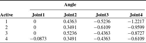
Table I. Target expectation of joint angle for the second experiment.
3. Experiment
The error due to relaxation of the tubing, joints, and antagonistic muscles can be converted into the pulling line and joint angle states. Thus, this error function, fitted by the joint angle state and the pull wire state, is expected to portray the system error model. There are many problems with these samples, such as shocks and noise. Excessive shocks and noise can affect the network fit and require preprocessing the data. The following are the steps to refine the MS model:
-
Combining the friction function state and the cable relaxation state into the state space of the torque error model.
-
Conduct the first friction compensation experiment and record the joint driving torque.
-
Identifying the weights and thresholds of the feedforward compensation model.
-
Testing the accuracy of the feedforward compensation model for torque compensation under the four desired actions in Table I.
-
Return to step 1 to change the state space combination until the model can achieve high accuracy.
3.1. The trajectory tracking experiment of the robot arm
The proportional–integral–derivative (PID) method was used in the first experiment, as shown in Fig. 3. The input is the desired muscle force $F_{ex}$
, and the output is the joint angles
$F_{ex}$
, and the output is the joint angles $q_{MS}$
, and angular velocity
$q_{MS}$
, and angular velocity $\dot{q}_{MS}$
.
$\dot{q}_{MS}$
. $\delta F$
is the force error of the skeletal system. The control frequency of the first experiment was 250 Hz, and the four joint angles of the robot arm were called Joint1, Joint2, Joint3, and Joint4, and the expected travels were
$\delta F$
is the force error of the skeletal system. The control frequency of the first experiment was 250 Hz, and the four joint angles of the robot arm were called Joint1, Joint2, Joint3, and Joint4, and the expected travels were $[{-}0.0703,-0.0979,-0.3104,-0.9258]rad$
.
$[{-}0.0703,-0.0979,-0.3104,-0.9258]rad$
.

Figure 3. The control block diagram without feedforward compensation.
A 20-s trajectory tracking task was repeated 14 times for a total of 280 s of experimentation, and the feedback signal is shown in Fig. 4. The error estimation network was trained using this experimental state.

Figure 4. The joint angle obtained without feedforward compensation.
Subsequently, $70\%$
of the data recorded in the first experiment was used for network training,
$70\%$
of the data recorded in the first experiment was used for network training, $70\%$
for validation, and
$70\%$
for validation, and $15\%$
for testing. The trained model has used the second experiment as a feedforward compensation module.
$15\%$
for testing. The trained model has used the second experiment as a feedforward compensation module.
In the second experiment, a human-like control method that considers contractile muscle dynamics has been used to realize path-tracking tasks on the MS, and a feedforward compensation module has been added, and the control block diagram is shown in Fig. 5.

Figure 5. Control block diagram of the bionic MS with feedforward compensation.
The bionic MS contains a 3-DOF shoulder joint and 1-DOF elbow joint. The shoulder joint is driven by seven muscles. Two muscles drive the elbow joint for 1 DOF of rotation of the forearm. Since the muscle force space is redundant, especially for the shoulder joint, and it is necessary to ensure that the values of the muscle forces are within a reasonable range. Convex optimization theory was used to solve the mapping problem between the errors in the joint moments and the errors in the muscle forces. The final activation signal compensation value is obtained from the inverse muscle model.
The second experiment contained four groups of movements, and a total of 53 experiments were performed for 20 s each, for a total of 1060 s of experiments. Fourteen times were randomly selected, as shown in Fig. 6.

Figure 6. The joint angle obtained with feedforward compensation.
The trajectory of the robotic arm without feedforward compensation control is shown in Fig. 7. The trajectory of the robotic arm with feedforward compensation control is shown in Fig. 8.

Figure 7. Trajectory tracking without feedforward compensation.
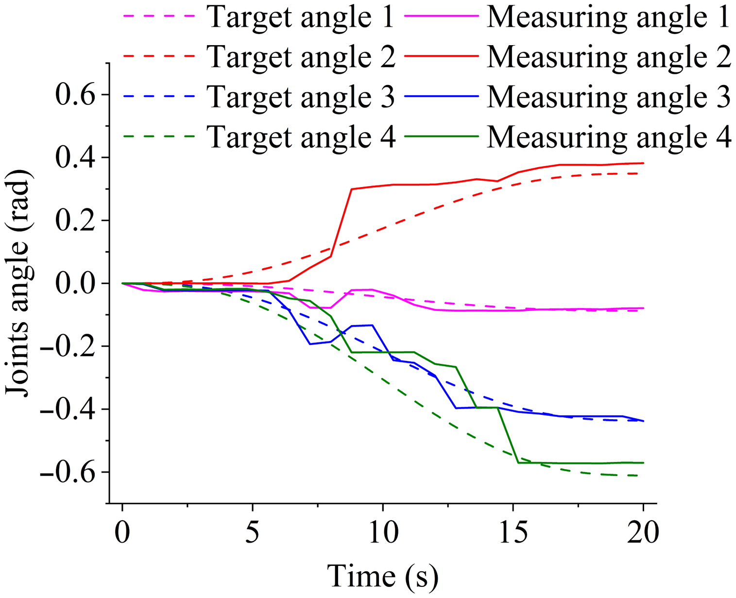
Figure 8. Trajectory tracking with feedforward compensation.
In Fig. 7, when the motion ends, the end position of the robotic arm, compared to the desired position, has an error of 147.1 mm, and this error accounts for $31.49\%$
of the total displacement. In Fig. 8, the error is 11.2 mm, which is
$31.49\%$
of the total displacement. In Fig. 8, the error is 11.2 mm, which is $5.83\%$
of the total displacement of the robotic arm.
$5.83\%$
of the total displacement of the robotic arm.
3.2. Feedforward control with compensated kinetic model
The product of the incremental arc of the encoder on the motor and the radius of the winch reflects the valid length of the muscle. The theoretical length of the muscle is derived by calculating the muscle attachment point distance from the joint angle. Calculate the travel error of a specific action motor encoder and the force point to get the error percentage. It can be intuitively perceived that the overall error of the second experiment is relatively tiny.
The experiment was repeated 14 times to record the state of the cable. The 14 results were analyzed to give the absolute travel errors of the motor encoder and force points, as well as the mean and standard deviation of the absolute errors. The error reflects the degree of difference of the cable at the end of the movement and is a dimensionless error. The mean and variance percentage of the error of 14 experiments between the calculated cable action point displacement and the cable displacement are shown in Fig. 9.

Figure 9. Statistical results after the first to $14$
th trials.
$14$
th trials.
In the experiments without feedforward compensation, the difference between the valid length of the cable and the theoretical length as a percentage of the theoretical length was $1.22\% \sim 11.43\%$
, and the standard deviation was
$1.22\% \sim 11.43\%$
, and the standard deviation was $0.48\% \sim 2.52\%$
. In the experiments with feedforward compensation, the difference between the actual length and the theoretical length of the cable as a percentage of the theoretical length was
$0.48\% \sim 2.52\%$
. In the experiments with feedforward compensation, the difference between the actual length and the theoretical length of the cable as a percentage of the theoretical length was $0.03\% \sim 2.09\%$
, and the standard deviation was
$0.03\% \sim 2.09\%$
, and the standard deviation was $0.01\% \sim 0.82\%$
.
$0.01\% \sim 0.82\%$
.
3.3. Results
The results show that the feedforward compensation module can reduce the tracking error between the desired and actual movements under the PID controller. It is demonstrated that the difference between the actual length and the theoretical length of the cable as a percentage of the theoretical length and its standard deviation is smaller in the experiment with feedforward compensation compared to the experiment without feedforward compensation. This indicates that the PID control with the feedforward compensation module can reduce the relaxation of the cable.
4. Conclusion
A feedforward compensation approach for friction fitted by a neural network is proposed for the problem of friction generated by the contact between the cable and the restraining structure/tube during muscle force transfer. The relaxation model of the cable is proposed for the problem that the cable can only transmit tension and antagonize the excessive relaxation/tension of the cable between the artificial muscles, and the mapping relationship between the joint space and the muscle space is given. In the hardware platform, the control model of the MS is established, and the trajectory tracking control verification is completed. In future work, it will be possible to introduce neural mechanisms and establish control methods consistent with biological properties
Acknowledgment
This work is supported partly by the National Key Research and Development Program of China (2017YFB1300203), partly by the National Natural Science Foundation of China (NSFC) (under Grants 61627808, 91648205), partly by the Strategic Priority Research Program of Chinese Academy of Science under Grant XDB32000000.
Authors contribution
Yerui Fan contributes to the main part of this paper. He takes a great part in the problem formulation and makes an analysis of the results. He does a large number of experiments in physical platforms. He mainly writes this paper. Jianbo Yuan designed the physical platform and also did some physical experiments. Yaxiong Wu gave some experimental opinions and improvement plans. Hong Qiao is in charge of this work and makes suggestive comments, which help a lot to improve the quality of this paper.
Declaration
This paper has been submitted to the ARM conference and has been recommended by the conference committee to submit to Robotica Journal. All work does not violate ethical standards. The author(s) declared no potential confficts of interest.


