


1. Introduction
In the last two decades, there has been a significant interest in autonomous robotics spacecrafts equipped with the tools, technologies, and techniques (i) to extend satellite(s)’ lifespan – even if they were not designed to be serviced on orbit and (ii) to assemble large space structures and manufacture on orbit. These on-orbit robotics capabilities will eliminate volume limits imposed by launch vehicles and replace some astronaut extravehicular activity tasks with precision robotics. Thus, on-orbit robotics servicing and assembly are deemed to be a key solution and technology due to existing launch & deployment constraints. These robotics technologies will also enable new architectures and capabilities for a wide range of government and commercial missions including in-space construction of large space structures, communications antennae, and telescopes.
Recently, OSAM-1 (formerly known as Restore-1), a robotics spacecraft, is being jointly developed by NASA and MAXAR Technologies Inc. and soon it will be ready to carry out various on-orbit assembly and servicing tasks such as fabrication, assembly of antennas, and refueling of satellites. ARCHINAUT (OSAM-2) developed by NASA and Made in Space Inc. features multiple robotics arms for on-orbit precision manufacturing and assembly [1–Reference Krebs-Gunter3]. Some other examples include the Gateway Moon Space Station by NASA and international partners, Moon Village and Mars Exploration by the European Space Agency, the OrbitalHub by the German Space Agency, and many other large space structures and telescopes [4].
On-orbit robotics servicing and assembly missions [Reference Flores-Abad, Ma, Pham and Ulrich5] generally include several modes of operations such as (a) orbital approach and rendezvous, (b) robotics arms deployment and pre-contact approach, (c) contact and capture, and (d) post-capture operations.
In the pre-contact stage, space manipulators mounted on the chaser spacecraft approach and gradually follow the motion of the target payload. In the contact stage, the space robots are free floating. Finally, during the post-capture phase, space robots suppress the target’s uncontrolled motion and establish a new trajectory [Reference Xu, Peng, Liang and Mu6, Reference Xu, Liang and Xu7]. Matsumoto et al. [Reference Matsumoto, Jacobsen, Dubowsky and Ohkami8] proposed the use of the natural dynamics to complete a passive fly-by approach and an optimal trajectory for close-range rendezvous with a rotating satellite. The study also considered issues such as collision avoidance between the manipulator and the target satellite. Ma et al. [Reference Ma, Ma and Shashikanth9] designed an optimal trajectory for a spacecraft to approach a tumbling satellite by minimizing time and fuel. A cubic spline-based collision avoidance algorithm for a robotics spacecraft was developed by Fejzic [Reference Fejzic10]. Xin and Pan [Reference Xu, Liang, Li and Xu11] developed an optimal control of spacecraft approaching a tumbling target. They minimized the flexible motion induced by large angular maneuvers using a non-linear optimal control technique. Vafa and Dubowsky [Reference Vafa and Dubowsky12] proposed a special cyclic motion trajectory of a manipulator’s joints to change the base spacecraft’s orientation. The path planning problem of a free-floating target with a manipulator having angular momentum was addressed by Yamada et al. in ref. [Reference Yamada13, Reference Yamada, Yoshikawa and Fujita14].
Gasbarri [Reference Gasbarri and Pisculli15] reported that the dynamics modeling and pre-contact motion planning of a space robot are significantly more complicated than those of fixed-base manipulators due to the “dynamic coupling” between the manipulator arms and the base platform. The study investigated pre-contact and post-capture phases and proposed a scheme to control either joint torques or moments applied to the chaser spacecraft.
The issue of stability and control during the initial stage of contact and capture has been extensively studied and published. Cyril [Reference Cyril, Misra, Ingham and Jaar16] developed a dynamics model of the compound system for a post-capture phase and proposed a model-based feedback linearization control scheme. Dimitrov [Reference Dimitrov and Yoshida17] presented two new control laws regarding management of the total angular momentum of a compound system during a post-capture phase. Wang [Reference Wang, Huang and Meng18] also emphasized on the post-capture phase and presented a novel sliding mode control scheme for a tether-connected robotics system.
Suresh [Reference Suresh and Kelkar19] presented a robust control theory based on a dissipative function for a stable compound system during an autonomous capture. Aghili [Reference Aghili20] developed a control model which dissipated unwanted linear and angular momentum to bring a tumbling target spacecraft to rest. Xu [Reference Xu, Li, Liang, Xu, Liu and Qiang21] proposed a control strategy to maneuver the captured spacecraft along with the mounted space robot during deployment of a target spacecraft. Cheah [Reference Cheah, Kawamura and Arimoto22] proposed a feedback control law which can deal with uncertain system parameters and still unload the angular momentum of the compound system. Dixon [Reference Dixon23] presented an adaptive regulation in the case of uncertain dynamics parameters of space robots. Cheah [Reference Cheah, Liu and Slotine24] developed an approximate Jacobian adaptive control scheme for robots. Wang [Reference Wang, Huang and Meng25] presented a Jacobian adaptive controller for free-floating space robots. Zhang [Reference Zhang, Liang, Wang, Mi, Zhang and Chen26] developed a modified adaptive sliding mode control algorithm to reduce the unknown angular momentum of a target spacecraft.
Schneider [Reference Schneider and Cannon27] studied a modified impedance control technique called Object Impedance Control for fixed-base multiple robots manipulating a common object. In this study, the common object followed a reference mechanical impedance. More recently, Moosavian [Reference Moosavian, Rastegari and Papadopoulos28] developed the Multiple Impedance Control algorithm for several cooperating robots which manipulate a common payload.
The Model Predictive Control (MPC) framework simultaneously allows optimization of the given performance index in conjunction with the accounting of the system dynamics and constraints as demonstrated in [Reference Vukov, Gros, Horn, Frison, Geebelen, Jørgensen, Swevers and Diehl29–Reference Fin34]. In a study conducted by Gangapersaud et al. [Reference Gangapersaud, Liu and de Ruiter35], a novel detumbling strategy is presented to detumble targets without prior knowledge of their inertial parameters. Detumbling of the target is achieved by controlling the space robot to follow a reference force/torque that is designed to detumble the target while respecting force/torque limits at the end-effector, without the use of the target’s inertial parameters. To ensure a stable detumbling strategy, a robust compensator is developed predicated on bounds of the target’s unknown inertial parameters.
One of the most practical and theoretical challenges in implementing a robust model of MPC is the ability to tackle the various uncertainties that can affect the performance of the system. Due to the receding horizon nature of the model, standard MPC can provide a level of robustness that is not available in other methods [Reference Shuyou, Marcus, Hong and Frank36]. Unfortunately, the literature showed that the standard MPC cannot provide adequate performance in complicated robotics systems [Reference Wei, Shen and Shi37]. To address this issue, many research efforts have been carried out on developing robust MPC that can provide robust stability and constraint satisfaction in the presence of uncertainties [Reference Wei, Sun, Chen and Shi38–Reference Ladoiye, Necsulescu and Sasiadek42]. Over the last few years, the scope and the real-time capabilities of Non-linear Model Predictive Control (NMPC) have been greatly improved. There has been remarkable increase in the number of tools that enable fast solutions of the various non-linear programs, such as gradient use (Englert et al. [Reference Englert, a. Volz, Rhein and Graichen43]), input parameterization. (Rathai [Reference Rathai44]), and real-time iterations (Quirynen et al. [Reference Quirynen, Vukov, Zanon and Diehl45]). The application of NMPS for free-floating space manipulator is provided in refs. [Reference Aghili46–Reference Rybus, Seweryn and Sasiadek48].
However, regardless of the applied control theory, it is observed that one of the most crucial problems and technical challenges for spacecraft robotics in the literature [Reference Wang, Luo and Walter49] is the saturation of force and torque of robot joint and spacecraft actuators during the post-capture stage while controlling a target spacecraft due to its uncontrolled large angular and linear momentums. In the literature [Reference Morato, Normey-Rico and Sename50], the manipulator damps out the target’s angular and linear momentums as quickly as possible subject to the constraint that the magnitude of the exerted force and torque remain below their prespecified values in the post-capture phase.
This paper directly focuses on the very issue and presents a novel solution with two robust and efficient control algorithms which minimize the joint torques and contact forces while maintaining the desired trajectory of the payload (i.e., target spacecraft) during the post-capture phase.
The literature to date in the area of application of MPC to robotics mainly focuses on linear models but the dual arm coordination is highly non-linear, and there is no robust MPC application on dual arm coordination. The proposed discretized technique offers exact realizations (of a non-linear model) with elegance and simplicity and yet takes into account the full non-linear model of the dual arm coordinating system. Furthermore, the cost function selected in NMPC is unique focusing on a practical problem, that is minimization of joint and spacecraft actuators moments during a post-capture phase while unloading momentum and bringing a target spacecraft to rest. In addition, the method is further extended to accommodate the pre-contact phase as well by simply changing the cost function to incorporate the minimum joint rates.
As far as the spacecraft hardware and software implementations are concerned, the space community is divided on the matter of centralized versus distributed processor architecture [Reference Sebestyen51]. After evaluating the proposed control algorithms, we have determined that a distributed architecture is the optimal choice for our application. This architecture offers several benefits, including parallel control of the spacecraft and robots, reduced computer speed demands, and enhanced reliability through inherent redundancy. Our proposed architecture consists of three main processors: (i) Spacecraft Attitude Determination and Control System (ADACS) and Robot Control System (RCS), (ii) Command and Data Handling (C&DH), and (iii) Communications Processor.
The control algorithm resides in the ADACS & RCS computer, responsible for controlling the spacecraft’s 3-axis momentum attitude, orbital maneuvers, and end-effector position and orientation control of the robots. The algorithm will also collect sensory data from sources such as the star trackers, joint encoders, and the vision system, among others. A star tracker allows for precise control of the spacecraft’s attitude, with accuracy of 0.01° or better. The spacecraft is equipped with three orthogonal reaction wheels and a combination of torque rods and magnetometer. The vision system determines the pose of the target spacecraft. The Computer Software Configuration Items (CSCIs) include a range of modules, such as OCA, NMPC, Forward and Inverse Kinematics Functions, the Robot Dynamics Function, Jacobian, Jacobian Rate, Impedance Control Trajectory Generation Function, and more. These CSCIs are located in the ADACS and RCS computer.
Section 2 presents the theoretical formulations, including the kinematics, dynamics model of the compound system which consists of a chaser spacecraft and two n-degree redundant manipulators and a target spacecraft. Two generic optimal control algorithms (utilizing (i) only the current states OCA or (ii) the current and the future predicted states – NMPC) are formulated to obtain optimal control actions for joint torques and the contact force/moments, respectively, to minimize a specified performance index.
Simulation results and discussion are presented in Section 3, and some concluding remarks are provided in Section 4.
2. Theoretical formulations
2.1. Description of the system
The system under consideration consists of a rigid spacecraft (chaser), two n-DOF redundant manipulators, and a rigid payload (target). An example of the system of a rigid spacecraft with two n-degree robots and a rigid payload is illustrated in Fig. 1(a). The geometry of the robotics arm is presented in Fig. 1(b–c). The parameters of the spacecraft robotics system used in the simulations are provided in Table I in Appendix.
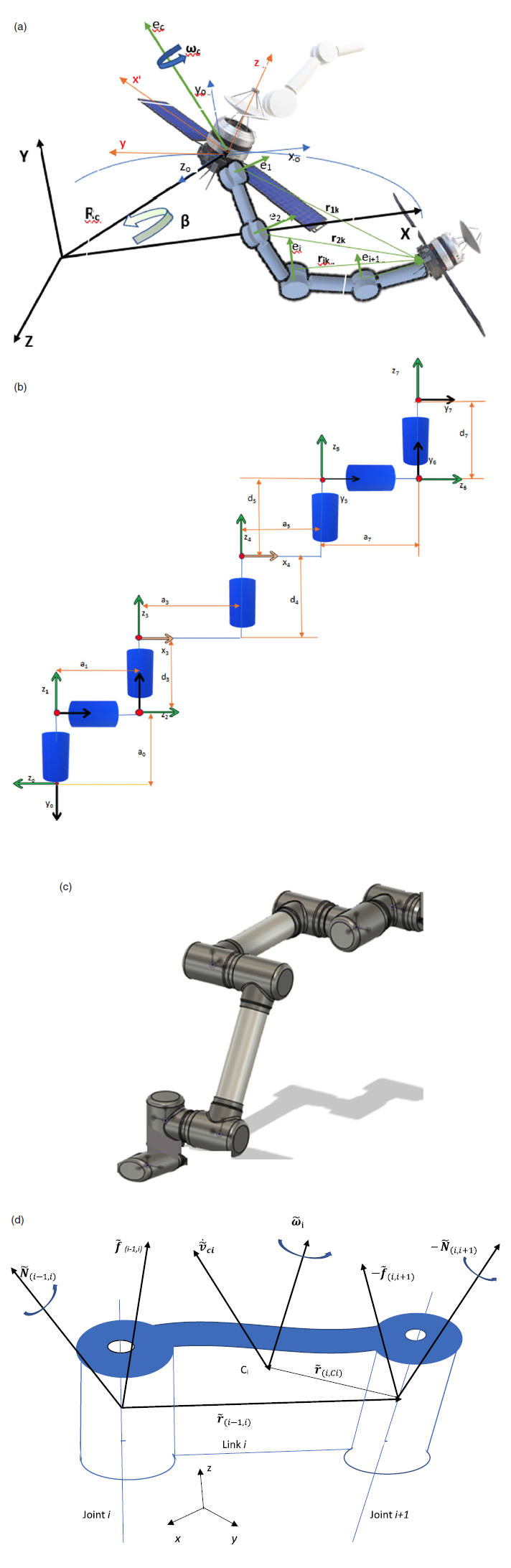
Figure 1. (a) The geometry and description of the system. (b) The robot arm geometry. (c) The 3-D robot arm model. (d) Free body diagram of link i.
Let the $\tilde{\boldsymbol{R}}_{\boldsymbol{c}}$
, the position vector and true anomaly β, define the location of the instantaneous center of mass C of the spacecraft with respect to the inertial coordinate system, X, Y, Z having its origin at the center of Earth. It is assumed that the inertial coordinate system is set up with x-axis pointing to perigee and z-axis to orbit normal, and the y-axis completes the right-hand triad.
$\tilde{\boldsymbol{R}}_{\boldsymbol{c}}$
, the position vector and true anomaly β, define the location of the instantaneous center of mass C of the spacecraft with respect to the inertial coordinate system, X, Y, Z having its origin at the center of Earth. It is assumed that the inertial coordinate system is set up with x-axis pointing to perigee and z-axis to orbit normal, and the y-axis completes the right-hand triad.
The motion is described by using a set of coordinate axes x, y, z fixed to the central body such that they are roll, pitch, and yaw axes, respectively. These in turn are obtained from a set of orbital coordinates axes x o, y o, z o through three rotations as described in Section 2.2. Here z o-axis is directed towards the center of Earth, y o-axis is along the orbit normal, and x o-axis completes the right-hand triad. For convenience, a set of local coordinates is also assigned to each joint of the robot manipulators where z i is parallel to the axis of rotation and x i is along the link and y i completes the right-hand triad.
2.2. Kinematics of the system
The rotational transformation from orbital to body axes is represented by a 1-3-2 Euler sequence, with angles φ, ψ, and θ, respectively. The components of the body-attached angular velocity along x, y, z axes can be written in terms of $\dot{\varphi }$
,
$\dot{\varphi }$
, $\dot{\psi }$
,
$\dot{\psi }$
, $\dot{\theta }$
as follows [Reference Craig52, Reference Rouki, Kalaycioglu and Patel53]
$\dot{\theta }$
as follows [Reference Craig52, Reference Rouki, Kalaycioglu and Patel53]
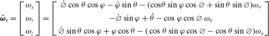 \begin{equation}\tilde{\boldsymbol{\omega }}_{\boldsymbol{c}}=\left[\begin{array}{c} \omega _{x}\\ \\[-8pt] \omega _{y}\\ \\[-8pt] \omega _{z} \end{array}\right]=\left[\begin{array}{c} \dot{{\varnothing }}\cos \theta \cos \varphi -\dot{\varphi }\sin \theta -({\cos }{\theta }\sin \varphi \cos \varnothing +\sin \theta \sin \varnothing )\omega _{o} \\ \\[-8pt] -\dot{{\varnothing }}\sin \varphi +\dot{\theta }-\cos \varphi \,{ \cos\varnothing }\, {\omega}_{\textrm{o}}\\ \\[-8pt] \dot{{\varnothing }}\sin \theta \cos \varphi +\varphi \cos \theta -(\cos \theta \sin \varphi \cos {\varnothing }-\cos \theta \sin \varnothing )\omega _{o} \end{array}\right] \end{equation}
where $\omega _{o}$
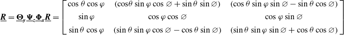
is the orbital angular velocity The transformation matrix
$\omega _{o}$
is the orbital angular velocity The transformation matrix $\underline{\boldsymbol{R}}$
which describes the relative rotational motion between the orbital coordinate frame (x
o, y
o, z
o) and the spacecraft attached coordinate frame (x, y, z) can be written as:
$\underline{\boldsymbol{R}}$
which describes the relative rotational motion between the orbital coordinate frame (x
o, y
o, z
o) and the spacecraft attached coordinate frame (x, y, z) can be written as:
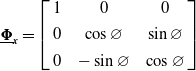 \begin{equation}\underline{\boldsymbol{\Phi }}_{\boldsymbol{x}}=\left[\begin{array}{c@{\quad}c@{\quad}c} 1 & 0 & 0\\ \\[-8pt] 0 & \cos \varnothing & \sin \varnothing \\ \\[-8pt] 0 & -\sin \varnothing & \cos \varnothing \end{array}\right]\end{equation}
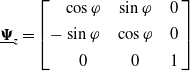 \begin{equation}\underline{\boldsymbol{\Psi }}_{\boldsymbol{z}}=\left[-\begin{array}{c@{\quad}c@{\quad}c} \cos \varphi & \sin \varphi & 0\\ \\[-8pt] \sin \varphi & \cos \varphi & 0\\ \\[-8pt] 0 & 0 & 1 \end{array}\right]\end{equation}
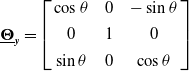 \begin{equation}\underline{\boldsymbol{\Theta }}_{\boldsymbol{y}}=\left[\begin{array}{c@{\quad}c@{\quad}c} \cos \theta & 0 & -\sin \theta \\ \\[-8pt] 0 & 1 & 0\\ \\[-8pt] \sin \theta & 0 & \cos \theta \end{array}\right]\end{equation}
The transformation matrix $\underline{\boldsymbol{B}}$
which defines the rotational motion from the inertial coordinates frame X, Y, Z to the orbital coordinate frame (x
o, y
o, z
o) can be calculated as follows:
$\underline{\boldsymbol{B}}$
which defines the rotational motion from the inertial coordinates frame X, Y, Z to the orbital coordinate frame (x
o, y
o, z
o) can be calculated as follows:
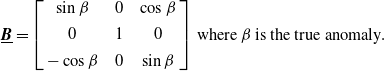 \begin{equation}\underline{\boldsymbol{B}}=\left[\begin{array}{c@{\quad}c@{\quad}c} \sin \beta & 0 & \cos \beta \\ \\[-8pt] 0 & 1 & 0\\ \\[-8pt] -\cos \beta & 0 & \sin \beta \end{array}\right]\,\text{where}\,\beta\, \text{is the true anomaly}.\end{equation}
These transformation matrices are obtained for both the target and chaser spacecrafts. Similarly, each homogeneous transformation matrix $\underline{\boldsymbol{T}_{\boldsymbol{i}}^{\boldsymbol{j}}}$
that transforms the coordinates of a point from frame j to frame i on a robot manipulator is calculated using Denavit-Hartenberg (D-H) convention [Reference Craig52, Reference Kalaycioglu and de Ruiter54].
$\underline{\boldsymbol{T}_{\boldsymbol{i}}^{\boldsymbol{j}}}$
that transforms the coordinates of a point from frame j to frame i on a robot manipulator is calculated using Denavit-Hartenberg (D-H) convention [Reference Craig52, Reference Kalaycioglu and de Ruiter54].
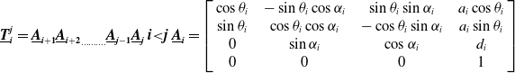
where the quantities $d_{i}, a_{i}, \theta _{i}, \alpha _{i},$
are parameters of link i and joint-i and
$d_{i}, a_{i}, \theta _{i}, \alpha _{i},$
are parameters of link i and joint-i and $a_{i},$
is the length of the link,
$a_{i},$
is the length of the link, $d_{i}$
is the offset,
$d_{i}$
is the offset, $\theta _{i}$
is the joint angle while
$\theta _{i}$
is the joint angle while $\alpha _{i}$
is the twist.
$\alpha _{i}$
is the twist.
The Jacobian matrices and their first-time derivatives between the center of the chaser spacecraft and a point k on the left robotics manipulator are as follows:
 \begin{equation}\left(\underline{\boldsymbol{J}}_{\boldsymbol{c}}^{\boldsymbol{k}}\right)_{\boldsymbol{L}}=\left[\begin{array}{c@{\quad}c@{\quad}c@{\quad}c@{\quad}c@{\quad}c@{\quad}c@{\quad}c} \widetilde{\boldsymbol{e}_{\boldsymbol{c}}} & \widetilde{\boldsymbol{e}_{\textbf{1}}} & \widetilde{\boldsymbol{e}_{\textbf{2}}} & \widetilde{\boldsymbol{e}_{\textbf{3}}} & \widetilde{\boldsymbol{e}_{\textbf{4}}} & \ldots & & \widetilde{\boldsymbol{e}_{\textbf{7}}}\\ \\[-8pt] \widetilde{\boldsymbol{e}_{\boldsymbol{c}}}\times \tilde{\boldsymbol{r}}_{\boldsymbol{ck}} & \widetilde{\boldsymbol{e}_{\textbf{1}}}\times \tilde{\boldsymbol{r}}_{\textbf{1}\boldsymbol{k}} & \widetilde{\boldsymbol{e}_{\textbf{2}}}\times \tilde{\boldsymbol{r}}_{\textbf{2}\boldsymbol{k}} & \widetilde{\boldsymbol{e}_{\textbf{3}}}\times \tilde{\boldsymbol{r}}_{\textbf{3}\boldsymbol{k}} & \widetilde{\boldsymbol{e}_{\textbf{4}}}\times \tilde{\boldsymbol{r}}_{\textbf{4}\boldsymbol{k}} & \ldots & & \widetilde{\boldsymbol{e}_{\textbf{7}}}\times \tilde{\boldsymbol{r}}_{\textbf{7}\boldsymbol{k}} \end{array}\right]\end{equation}
 \begin{equation}\left(\underline{\dot{\boldsymbol{J}}}_{\boldsymbol{c}}^{\boldsymbol{k}}\right)_{\boldsymbol{L}}=\left[\begin{array}{c@{\quad}c@{\quad}c@{\quad}c@{\quad}c@{\quad}c@{\quad}c@{\quad}c} \widetilde{\boldsymbol{e}_{\boldsymbol{c}}} & \widetilde{\boldsymbol{e}_{\textbf{1}}} & & \ldots & \ldots & \ldots & \ldots & \widetilde{\boldsymbol{e}_{\textbf{7}}}\\ \\[-8pt] \widetilde{\boldsymbol{e}_{\boldsymbol{c}}}\times (\tilde{\boldsymbol{\omega }}_{\boldsymbol{c}}\times \tilde{\boldsymbol{r}}_{\boldsymbol{ck}}) & \widetilde{\boldsymbol{e}_{\textbf{1}}}\times (\dot{\theta }_{1L} \widetilde{\boldsymbol{e}_{\textbf{1}}}\times \tilde{\boldsymbol{r}}_{\textbf{1}\boldsymbol{k}}) & & \ldots & \ldots & \ldots & \ldots & \widetilde{\boldsymbol{e}_{\textbf{7}}}\times (\dot{\theta }_{7L}\widetilde{\boldsymbol{e}_{\textbf{7}}}\times \tilde{\boldsymbol{r}}_{\boldsymbol{ck}}) \end{array}\right]\end{equation}
where $\widetilde{\boldsymbol{e}_{\boldsymbol{c}}}$
is the unit vector along
$\widetilde{\boldsymbol{e}_{\boldsymbol{c}}}$
is the unit vector along $\tilde{\boldsymbol{\omega }}_{\boldsymbol{c}}$
spacecraft angular velocity vector,
$\tilde{\boldsymbol{\omega }}_{\boldsymbol{c}}$
spacecraft angular velocity vector, $\tilde{\boldsymbol{e}}_{\boldsymbol{i}}$
is the unit vector along the rotation axis of the ith joint and
$\tilde{\boldsymbol{e}}_{\boldsymbol{i}}$
is the unit vector along the rotation axis of the ith joint and $\tilde{\boldsymbol{r}}_{\boldsymbol{ck}}, \tilde{\boldsymbol{r}}_{\boldsymbol{ik}}$
are the displacement vectors from the center mass of the chaser spacecraft and ith joint to the point k, respectively. For example, if the Jacobian matrix between the center of the chaser spacecraft and the end-effector is selected, k will be assigned to (n + 1). Similarly, the Jacobian matrices and time derivatives can be calculated for the right manipulator.
$\tilde{\boldsymbol{r}}_{\boldsymbol{ck}}, \tilde{\boldsymbol{r}}_{\boldsymbol{ik}}$
are the displacement vectors from the center mass of the chaser spacecraft and ith joint to the point k, respectively. For example, if the Jacobian matrix between the center of the chaser spacecraft and the end-effector is selected, k will be assigned to (n + 1). Similarly, the Jacobian matrices and time derivatives can be calculated for the right manipulator.
The linear, angular velocities, and accelerations of any point on the left manipulator can be calculated by using the Jacobian matrix [Reference Kalaycioglu and de Ruiter54]:
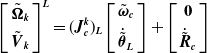 \begin{equation}\left[\begin{array}{c} \tilde{\boldsymbol{\Omega }}_{\boldsymbol{k}}\\ \\[-8pt] \tilde{\boldsymbol{V}}_{\boldsymbol{k}} \end{array}\right]^{\boldsymbol{L}}=({\boldsymbol{J}}_{\boldsymbol{c}}^{\boldsymbol{k}})_{\boldsymbol{L}}\left[\begin{array}{c} \tilde{\boldsymbol{\omega }}_{\boldsymbol{c}}\\ \\[-8pt] \dot{\tilde{\boldsymbol{\theta }}}_{\boldsymbol{L}} \end{array}\right]+\left[\begin{array}{c} \textbf{0}\\ \\[-8pt] \dot{\tilde{\boldsymbol{R}}}_{\boldsymbol{c}} \end{array}\right]\end{equation}
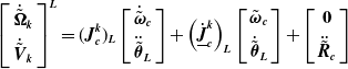 \begin{equation}\left[\begin{array}{c} \dot{\tilde{\boldsymbol{\Omega }}}_{\boldsymbol{k}}\\ \\[-8pt] \dot{\tilde{\boldsymbol{V}}}_{\boldsymbol{k}} \end{array}\right]^{\boldsymbol{L}}=({\boldsymbol{J}}_{\boldsymbol{c}}^{\boldsymbol{k}})_{\boldsymbol{L}}\left[\begin{array}{c} \dot{\tilde{\boldsymbol{\omega }}}_{\boldsymbol{c}}\\ \\[-8pt] \ddot{\tilde{\boldsymbol{\theta }}}_{\boldsymbol{L}} \end{array}\right]+\left(\underline{\dot{\boldsymbol{J}}}_{\boldsymbol{c}}^{\boldsymbol{k}}\right)_{\boldsymbol{L}}\left[\begin{array}{c} \tilde{\boldsymbol{\omega }}_{\boldsymbol{c}}\\ \\[-8pt] \dot{\tilde{\boldsymbol{\theta }}}_{\boldsymbol{L}} \end{array}\right]+\left[\begin{array}{c} \textbf{0}\\ \\[-8pt] \ddot{\tilde{\boldsymbol{R}}}_{\boldsymbol{c}} \end{array}\right]\end{equation}
where $\dot{\tilde{\boldsymbol{\theta }}}_{\boldsymbol{L}}^{\boldsymbol{T}}=[\dot{\theta }_{1L}, \dot{\theta }_{2L}, \dot{\theta }_{3L }\ldots \dot{\theta }_{n}]$
is the left-arm joint rates,
$\dot{\tilde{\boldsymbol{\theta }}}_{\boldsymbol{L}}^{\boldsymbol{T}}=[\dot{\theta }_{1L}, \dot{\theta }_{2L}, \dot{\theta }_{3L }\ldots \dot{\theta }_{n}]$
is the left-arm joint rates, $\tilde{\boldsymbol{V}}_{\boldsymbol{k}}$
and
$\tilde{\boldsymbol{V}}_{\boldsymbol{k}}$
and $\tilde{\boldsymbol{\Omega }}_{\boldsymbol{k}}$
are the (3×1) linear and angular velocity vectors of the k point on the left manipulator, respectively. Similarly, the linear and angular velocity of any point on the right manipulator can also be determined by simply changing the index from L to R.
$\tilde{\boldsymbol{\Omega }}_{\boldsymbol{k}}$
are the (3×1) linear and angular velocity vectors of the k point on the left manipulator, respectively. Similarly, the linear and angular velocity of any point on the right manipulator can also be determined by simply changing the index from L to R.
2.3. Dynamics model of the system
The dynamics equations are obtained by Newton-Euler formulation. Figure 1(d) shows all the forces and moments acting on link i.
The translational equation of motion is developed by adding the inertial force to the static balance of forces on each link so that
 \begin{equation}\tilde{\boldsymbol{f}}_{(i-1,i)}-\tilde{\boldsymbol{f}}_{(i,i+1)}-m_{i} \dot{\tilde{\boldsymbol{v}}}_{\boldsymbol{ci}}=\tilde{\textbf{0}}\ i=1,..,m\end{equation}
where $\tilde{\boldsymbol{f}}$
(i−1, i) and −
$\tilde{\boldsymbol{f}}$
(i−1, i) and − $\tilde{\boldsymbol{f}}$
(i, i + 1) are the coupling forces applied to link i by links i−1 and i + 1, respectively.
$\tilde{\boldsymbol{f}}$
(i, i + 1) are the coupling forces applied to link i by links i−1 and i + 1, respectively.
The inertial torque acting on link i is given by the time rate of change of the angular momentum of the link at that instant. Let $\tilde{\boldsymbol{\omega }}_{\textbf{i}}$
be the angular velocity vector and
$\tilde{\boldsymbol{\omega }}_{\textbf{i}}$
be the angular velocity vector and $\underline{\boldsymbol{I}_{\boldsymbol{i}}}$
be the centroidal inertia tensor of link i, then the angular momentum is given by
$\underline{\boldsymbol{I}_{\boldsymbol{i}}}$
be the centroidal inertia tensor of link i, then the angular momentum is given by $\underline{\boldsymbol{I}_{\boldsymbol{i}}}\tilde{\boldsymbol{\omega }}_{\textbf{i}}$
and the gyroscopic torque is calculated as
$\underline{\boldsymbol{I}_{\boldsymbol{i}}}\tilde{\boldsymbol{\omega }}_{\textbf{i}}$
and the gyroscopic torque is calculated as $\tilde{\boldsymbol{\omega }}_{{i}}$
×
$\tilde{\boldsymbol{\omega }}_{{i}}$
× $\underline{\boldsymbol{I}_{\boldsymbol{i}}}\tilde{\boldsymbol{\omega }}_{{i}}$
. Adding these terms to the static balance of moments yields
$\underline{\boldsymbol{I}_{\boldsymbol{i}}}\tilde{\boldsymbol{\omega }}_{{i}}$
. Adding these terms to the static balance of moments yields
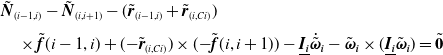 \begin{align} &\tilde{\boldsymbol{N}}_{(i-1,i)} - \tilde{\boldsymbol{N}}_{(i,i+1)} - (\tilde{\boldsymbol{r}}_{(i-1,i)} + \tilde{\boldsymbol{r}}_{(i,Ci)}) \nonumber\\[3pt]&\quad \times \tilde{\boldsymbol{f}}{(i-1,i)} + ({-}\tilde{\boldsymbol{r}}_{(i,Ci)}) \times ({-}\tilde{\boldsymbol{f}}{(i,i+1)}) - \underline{\boldsymbol{I}_{\boldsymbol{i}}}\dot{\tilde{\boldsymbol{\omega }}}_{\boldsymbol{i}} - {\tilde{\boldsymbol{\omega }}}_{\boldsymbol{i}} \times (\underline{\boldsymbol{I}_{\boldsymbol{i}}} {\tilde{\boldsymbol{\omega }}}_{\boldsymbol{i}}) =\tilde{\textbf{0}}\end{align}
where $\tilde{\boldsymbol{N}}_{(i-1,i)}$
and
$\tilde{\boldsymbol{N}}_{(i-1,i)}$
and $\tilde{\boldsymbol{N}}_{(i,i+1)}$
are the coupling moments and
$\tilde{\boldsymbol{N}}_{(i,i+1)}$
are the coupling moments and $\tilde{\boldsymbol{r}}_{(i-1,i)}$
,
$\tilde{\boldsymbol{r}}_{(i-1,i)}$
, $\tilde{\boldsymbol{r}}_{(i,Ci)}$
are the displacement vectors as shown in Fig. 1(d).
$\tilde{\boldsymbol{r}}_{(i,Ci)}$
are the displacement vectors as shown in Fig. 1(d).
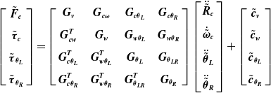
The complete set of equations for the two robots and the chaser spacecraft is obtained by evaluating both equations for all the links and the spacecraft, i = 1,⋯, m. To obtain closed-form dynamic equations, one can first eliminate the constraint forces and separate them from the joint torques, so as to explicitly involve the joint torques in the dynamic equations as follows [Reference Psomiadis and Papadopoulos47]:
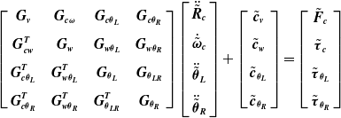 \begin{equation}\left[\begin{array}{c@{\quad}c@{\quad}c@{\quad}c} \boldsymbol{G}_{\boldsymbol{v}} & \boldsymbol{G}_{\boldsymbol{c}\boldsymbol{\omega }} & \boldsymbol{G}_{\boldsymbol{c}{\boldsymbol{\theta }_{\boldsymbol{L}}}} & \boldsymbol{G}_{\boldsymbol{c}{\boldsymbol{\theta }_{\boldsymbol{R}}}}\\ \\[-5pt] \boldsymbol{G}_{\boldsymbol{cw}}^{\boldsymbol{T}} & \boldsymbol{G}_{\boldsymbol{w}} & \boldsymbol{G}_{{\boldsymbol{w}\boldsymbol{\theta }_{\boldsymbol{L}}}} & \boldsymbol{G}_{{\boldsymbol{w}\boldsymbol{\theta }_{\boldsymbol{R}}}}\\ \\[-5pt] \boldsymbol{G}_{\boldsymbol{c}\boldsymbol{\theta }_{\boldsymbol{L}}}^{\boldsymbol{T}} & \boldsymbol{G}_{\boldsymbol{w}\boldsymbol{\theta }_{\boldsymbol{L}}}^{\boldsymbol{T}} & \boldsymbol{G}_{{\boldsymbol{\theta }_{\boldsymbol{L}}}} & \boldsymbol{G}_{{\boldsymbol{\theta }_{\boldsymbol{LR}}}}\\ \\[-5pt] \boldsymbol{G}_{\boldsymbol{c}\boldsymbol{\theta }_{\boldsymbol{R}}}^{\boldsymbol{T}} & \boldsymbol{G}_{\boldsymbol{w}\boldsymbol{\theta }_{\boldsymbol{R}}}^{\boldsymbol{T}} & \boldsymbol{G}_{\boldsymbol{\theta }_{\boldsymbol{LR}}}^{\boldsymbol{T}} & \boldsymbol{G}_{{\boldsymbol{\theta }_{\boldsymbol{R}}}} \end{array}\right]\left[\begin{array}{c} \ddot{\tilde{\boldsymbol{R}}}_{\boldsymbol{c}}\\ \\[-5pt] \dot{\tilde{\boldsymbol{\omega }}}_{\boldsymbol{c}}\\ \\[-5pt] \ddot{\tilde{\boldsymbol{\theta }}}_{\boldsymbol{L}}\\ \\[-5pt] \ddot{\tilde{\boldsymbol{\theta }}}_{\boldsymbol{R}} \end{array}\right]+\left[\begin{array}{c} \tilde{\boldsymbol{c}}_{\boldsymbol{v}}\\ \\[-5pt] \tilde{\boldsymbol{c}}_{\boldsymbol{w}}\\ \\[-5pt] \tilde{\boldsymbol{c}}_{{\boldsymbol{\theta }_{\boldsymbol{L}}}}\\ \\[-5pt] \tilde{\boldsymbol{c}}_{{\boldsymbol{\theta }_{\boldsymbol{R}}}} \end{array}\right]=\left[\begin{array}{c} \tilde{\boldsymbol{F}}_{\boldsymbol{c}}\\ \\[-5pt] \tilde{\boldsymbol{\tau }}_{\boldsymbol{c}}\\ \\[-5pt] \tilde{\boldsymbol{\tau }}_{{\boldsymbol{\theta }_{\boldsymbol{L}}}}\\ \\[-5pt] \tilde{\boldsymbol{\tau }}_{{\boldsymbol{\theta }_{\boldsymbol{R}}}} \end{array}\right]\end{equation}
where $\underline{\boldsymbol{G}}$
the mass/inertia matrix is a positive definite matrix and,
$\underline{\boldsymbol{G}}$
the mass/inertia matrix is a positive definite matrix and, $\dot{\tilde{\boldsymbol{R}}}_{\boldsymbol{c}}$
,
$\dot{\tilde{\boldsymbol{R}}}_{\boldsymbol{c}}$
, $\dot{\tilde{\boldsymbol{\omega }}}_{\boldsymbol{c}}$
are the linear and angular acceleration of the chaser spacecraft,
$\dot{\tilde{\boldsymbol{\omega }}}_{\boldsymbol{c}}$
are the linear and angular acceleration of the chaser spacecraft, $\ddot{\tilde{\boldsymbol{\theta }}}_{\boldsymbol{L}}$
,
$\ddot{\tilde{\boldsymbol{\theta }}}_{\boldsymbol{L}}$
, $\ddot{\tilde{\boldsymbol{\theta }}}_{\boldsymbol{R}}$
are the joint angular accelerations for the left and right arm, respectively.
$\ddot{\tilde{\boldsymbol{\theta }}}_{\boldsymbol{R}}$
are the joint angular accelerations for the left and right arm, respectively. $\tilde{\boldsymbol{c}}_{\boldsymbol{v}}$
,
$\tilde{\boldsymbol{c}}_{\boldsymbol{v}}$
, $\tilde{\boldsymbol{c}}_{\boldsymbol{w}}$
,
$\tilde{\boldsymbol{c}}_{\boldsymbol{w}}$
, $\tilde{\boldsymbol{c}}_{{\boldsymbol{\theta }_{\boldsymbol{L}}}}$
, and
$\tilde{\boldsymbol{c}}_{{\boldsymbol{\theta }_{\boldsymbol{L}}}}$
, and $\tilde{\boldsymbol{c}}_{{\boldsymbol{\theta }_{\boldsymbol{R}}}}$
are the non-linear terms while
$\tilde{\boldsymbol{c}}_{{\boldsymbol{\theta }_{\boldsymbol{R}}}}$
are the non-linear terms while $\tilde{\boldsymbol{F}}_{\boldsymbol{c}}, \tilde{\boldsymbol{\tau }}_{\boldsymbol{c}}$
are the external control force and moments for the chaser spacecraft and
$\tilde{\boldsymbol{F}}_{\boldsymbol{c}}, \tilde{\boldsymbol{\tau }}_{\boldsymbol{c}}$
are the external control force and moments for the chaser spacecraft and $\tilde{\boldsymbol{\tau }}_{{\boldsymbol{\theta }_{\boldsymbol{L}}}}$ $, \tilde{\boldsymbol{\tau }}_{{\boldsymbol{\theta }_{\boldsymbol{R}}}}$
are the joint control torques for the left and right arm, respectively.
$, \tilde{\boldsymbol{\tau }}_{{\boldsymbol{\theta }_{\boldsymbol{R}}}}$
are the joint control torques for the left and right arm, respectively.
2.4. Proposed optimal control techniques for dynamics control of coupled spacecraft attitude and robotics manipulators
The system consisting of two redundant manipulators and the two spacecrafts, namely the chaser and the target, is mathematically an underdetermined system due to the redundant number of actuators and sensors available to control the attitude and translational motions of the links and the spacecrafts.
This section presents a novel control solution to this problem by two control algorithms based on (i) Optimal Control Allocation OCA and (ii) Non-linear Model Predictive Control (NMPC). Both algorithms are aimed to minimize joint torques, spacecraft actuator moments, and contact forces moments of a compound redundant system which consists of a common payload (target spacecraft) grasped by dual n-degree space robotics manipulators mounted on a chaser spacecraft while tracking a desired trajectory. The OCA is based on optimal control allocation minimizing a quadratic cost function using the current state values and the system dynamics. On the other hand, the second NMPC algorithm minimizes a quadratic cost function which not only includes the current states but also the future state estimates, and the control inputs over a specified prediction horizon. The NMPC is deemed to be a natural extension of the OCA algorithm presented here and either technique can be employed based on availability of on-board computational resources.
2.4.1. The OCA formulation
The OCA algorithm involves two stages as demonstrated below in a control system block diagram in Fig. 2(a). The first stage of the control block diagram includes impedance control technique which is responsible for generating the desired trajectories for the end-effectors of the left and right robots prior to making a contact with the payload [Reference Kalaycioglu and de Ruiter54].
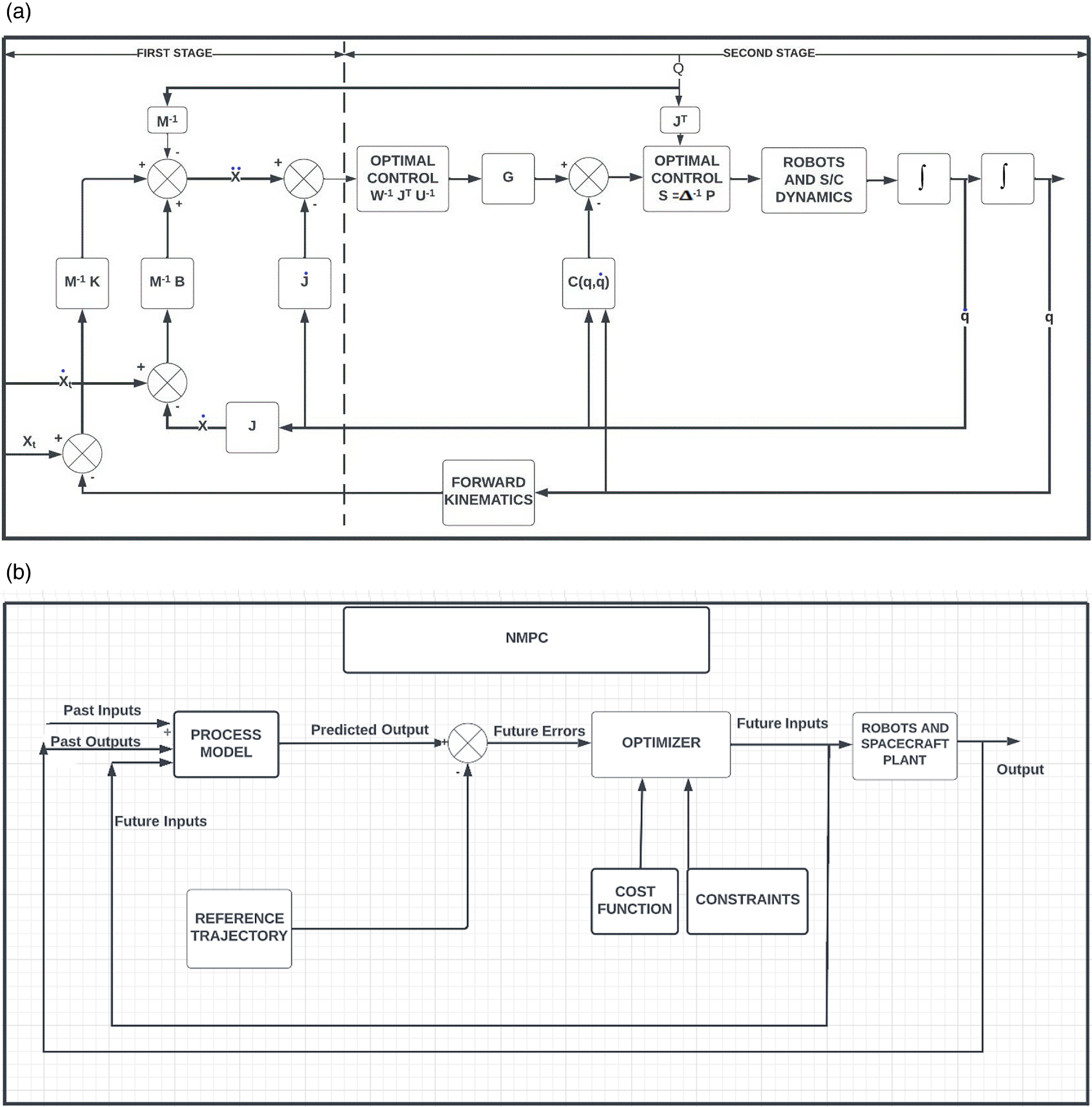
Figure 2. (a) Two-stage control system block diagram with OCA. (b) Non-linear model predictive control block (NMPC) diagram.
The second stage of the block diagram based on OCA algorithm is robust and computationally very efficient and provides minimum norm of joint torques and contact forces for an underdetermined compound robotics system. This technique was originally developed for cooperating rovers [Reference Sebestyen51]. The formulation is hereby extended to free-floating spacecraft-based cooperating space arms. In addition, it is further applied to two different modes of operations (i.e., pre-contact and post-capture) of space arms as presented below.
2.4.1.1. OCA pre-contact stage
This is the mode of operation where the two end-effectors approach toward the target spacecraft (i.e., payload). In a real space application, the relative motion of the target is determined via a vision or a laser system located on the robot end-effectors or on the capture spacecraft and thus the end-effectors approach to the vicinity of the payload’s grapple fixtures to grab the payload.
One can assume that the relative payload-grapple fixture trajectory, $\tilde{X}$
i-rel, is determined via the chaser spacecraft vision system. After transforming this information into the inertial reference frame, the following relationships can be written between the time derivatives of the pose of the left grapple fixture and the joint rates and angular rates of the chaser spacecraft using the Jacobian matrix and its time derivative.
$\tilde{X}$
i-rel, is determined via the chaser spacecraft vision system. After transforming this information into the inertial reference frame, the following relationships can be written between the time derivatives of the pose of the left grapple fixture and the joint rates and angular rates of the chaser spacecraft using the Jacobian matrix and its time derivative.
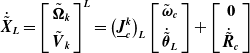 \begin{equation}\dot{\tilde{\boldsymbol{X}}}_{\boldsymbol{L}}=\left[\begin{array}{c} \tilde{\boldsymbol{\Omega }}_{\boldsymbol{k}}\\ \\[-8pt] \tilde{\boldsymbol{V}}_{\boldsymbol{k}} \end{array}\right]^{\boldsymbol{L}}=\left(\underline{\boldsymbol{J}}_{\boldsymbol{c}}^{\boldsymbol{k}}\right)_{\boldsymbol{L}}\left[\begin{array}{c} \tilde{\boldsymbol{\omega }}_{\boldsymbol{c}}\\ \\[-8pt] \dot{\tilde{\boldsymbol{\theta }}}_{\boldsymbol{L}} \end{array}\right]+\left[\begin{array}{c} \textbf{0}\\ \\[-8pt] \dot{\tilde{\boldsymbol{R}}}_{\boldsymbol{c}} \end{array}\right]\end{equation}
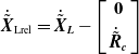 \begin{equation}\dot{\tilde{\boldsymbol{X}}}_{\boldsymbol{\textrm{Lrel}}}=\dot{\tilde{\boldsymbol{X}}}_{\boldsymbol{L}}-\left[\begin{array}{c} \textbf{0}\\ \\[-8pt] \dot{\tilde{\boldsymbol{R}}}_{\boldsymbol{c}} \end{array}\right]\end{equation}
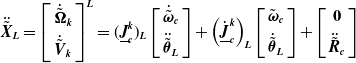 \begin{equation}\ddot{\tilde{\boldsymbol{X}}}_{\boldsymbol{L}}=\left[\begin{array}{c} \dot{\tilde{\boldsymbol{\Omega }}}_{\boldsymbol{k}}\\ \\[-8pt] \dot{\tilde{\boldsymbol{V}}}_{\boldsymbol{k}} \end{array}\right]^{\boldsymbol{L}}=(\underline{\boldsymbol{J}}_{\boldsymbol{c}}^{\boldsymbol{k}})_{\boldsymbol{L}}\left[\begin{array}{c} \dot{\tilde{\boldsymbol{\omega }}}_{\boldsymbol{c}}\\ \\[-8pt] \ddot{\tilde{\boldsymbol{\theta }}}_{\boldsymbol{L}} \end{array}\right]+\left(\underline{\dot{\boldsymbol{J}}}_{\boldsymbol{c}}^{\boldsymbol{k}}\right)_{\boldsymbol{L}}\left[\begin{array}{c} \tilde{\boldsymbol{\omega }}_{\boldsymbol{c}}\\ \\[-8pt] \dot{\tilde{\boldsymbol{\theta }}}_{\boldsymbol{L}} \end{array}\right]+\left[\begin{array}{c} \textbf{0}\\ \\[-8pt] \ddot{\tilde{\boldsymbol{R}}}_{\boldsymbol{c}} \end{array}\right]\end{equation}
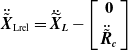 \begin{equation}\ddot{\tilde{\boldsymbol{X}}}_{\boldsymbol{\textrm{Lrel}}}=\ddot{\widetilde{ \boldsymbol{X}}}_{\boldsymbol{L}}-\left[\begin{array}{c} \textbf{0}\\ \\[-8pt] \ddot{\tilde{\boldsymbol{R}}}_{\boldsymbol{c}} \end{array}\right]\end{equation}
where $\boldsymbol{k}$
refers to the location of the left grapple fixture,
$\boldsymbol{k}$
refers to the location of the left grapple fixture, $\check {X}_{L}$
and
$\check {X}_{L}$
and $\tilde{X}$
Lrel are the absolute and the relative displacement vectors, respectively. Similar relations exist for the right grapple fixture.
$\tilde{X}$
Lrel are the absolute and the relative displacement vectors, respectively. Similar relations exist for the right grapple fixture.
During the pre-contact stage, the end-effectors are in a free motion (i.e., holding no common payload) and the system consists of a tree structure. The following cost function, $C_{o}$
is employed to obtain the minimum norm joint and Euler angular rates:
$C_{o}$
is employed to obtain the minimum norm joint and Euler angular rates:
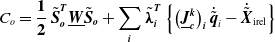 \begin{equation}C_{o}=\frac{\textbf{1}}{\textbf{2}}\,\tilde{\boldsymbol{S}}_{\boldsymbol{o}}^{\boldsymbol{T}}\underline{\boldsymbol{W}}\tilde{\boldsymbol{S}}_{\boldsymbol{o}}+\sum _{\boldsymbol{i}}\tilde{\boldsymbol{\lambda }}_{\boldsymbol{i}}^{\boldsymbol{T}}\left\{\left(\underline{\boldsymbol{J}}_{\boldsymbol{c}}^{\boldsymbol{k}}\right)_{\boldsymbol{i}}\dot{\tilde{\boldsymbol{q}}}_{i}-\dot{\tilde{\boldsymbol{X}}}_{\boldsymbol{\textrm{irel}}}\right\}\end{equation} $\underline{\boldsymbol{W}}$
is a square (3 + 2n, 3 + 2n) positive definite weighting matrix, n is being the total number of joints for each arm, and
$\underline{\boldsymbol{W}}$
is a square (3 + 2n, 3 + 2n) positive definite weighting matrix, n is being the total number of joints for each arm, and $\tilde{\boldsymbol{\lambda }}_{\boldsymbol{i}}^{\boldsymbol{T}}$
is the (6×1) Lagrangian multiplier and i is replaced by the L and R for the left and right robots, respectively.
$\tilde{\boldsymbol{\lambda }}_{\boldsymbol{i}}^{\boldsymbol{T}}$
is the (6×1) Lagrangian multiplier and i is replaced by the L and R for the left and right robots, respectively.
The $\dot{\tilde{\boldsymbol{q}}}$
and
$\dot{\tilde{\boldsymbol{q}}}$
and $\tilde{\boldsymbol{S}}_{\boldsymbol{o}}$
vectors which consist of the spacecraft angular as well as the left and right arm joint angular rates are provided below:
$\tilde{\boldsymbol{S}}_{\boldsymbol{o}}$
vectors which consist of the spacecraft angular as well as the left and right arm joint angular rates are provided below:
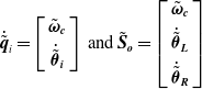 \begin{equation}\dot{\tilde{\boldsymbol{q}}}_{i}=\left[\begin{array}{c} \tilde{\boldsymbol{\omega }}_{\boldsymbol{c}}\\ \\[-8pt] \dot{\tilde{\boldsymbol{\theta }}}_{\boldsymbol{i}} \end{array}\right] \,\text{and} \,\tilde{\boldsymbol{S}}_{\boldsymbol{o}}=\left[\begin{array}{c} \tilde{\boldsymbol{\omega }}_{\boldsymbol{c}}\\ \\[-8pt] \dot{\tilde{\boldsymbol{\theta }}}_{\boldsymbol{L}}\\ \\[-8pt] \dot{\tilde{\boldsymbol{\theta }}}_{\boldsymbol{R}} \end{array}\right]\end{equation}
Minimizing the cost function $C_{o}$
with respect to
$C_{o}$
with respect to $\dot{\tilde{\boldsymbol{q}}}_{i}$
and
$\dot{\tilde{\boldsymbol{q}}}_{i}$
and $\tilde{\boldsymbol{\lambda }}_{\boldsymbol{i}}$
can be carried out by differentiating
$\tilde{\boldsymbol{\lambda }}_{\boldsymbol{i}}$
can be carried out by differentiating $C_{o}$
with respect to
$C_{o}$
with respect to $\dot{\tilde{\boldsymbol{q}}}_{i}$
and
$\dot{\tilde{\boldsymbol{q}}}_{i}$
and $\tilde{\boldsymbol{\lambda }}_{\boldsymbol{i}}$
(where i is replaced by L and R for the left and right robots, respectively), and one can calculate the minimum norm of joint and Euler rates as follows:
$\tilde{\boldsymbol{\lambda }}_{\boldsymbol{i}}$
(where i is replaced by L and R for the left and right robots, respectively), and one can calculate the minimum norm of joint and Euler rates as follows:
 \begin{equation}\frac{\partial C_{o}}{\partial \dot{\tilde{\boldsymbol{q}}}_{\boldsymbol{i}}}=\left\{\underline{\boldsymbol{W}}_{\boldsymbol{i}}\dot{\widetilde{ \boldsymbol{q}}}_{\boldsymbol{i}}+\left(\underline{\boldsymbol{J}}_{\boldsymbol{c}}^{\boldsymbol{k}}\right)_{\boldsymbol{i}}^{\boldsymbol{T}}\tilde{\boldsymbol{\lambda }}_{\boldsymbol{i}}\right\}=\tilde{\textbf{0}}\end{equation}
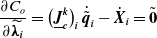 \begin{equation}\frac{\partial C_{o}}{\partial \widetilde{\boldsymbol{\lambda }_{\boldsymbol{i}}}}=\left(\underline{\boldsymbol{J}}_{\boldsymbol{c}}^{\boldsymbol{k}}\right)_{\boldsymbol{i}}\dot{\tilde{\boldsymbol{q}}}_{\boldsymbol{i}}-\dot{\boldsymbol{X}}_{\boldsymbol{i}}=\tilde{\textbf{0}}\end{equation}
Solving for $\dot{\tilde{\boldsymbol{q}}}_{i}$
from Eq. (16), one can obtain the following relationship:
$\dot{\tilde{\boldsymbol{q}}}_{i}$
from Eq. (16), one can obtain the following relationship:
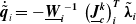 \begin{equation}\dot{\tilde{\boldsymbol{q}}}_{i}=-{\underline{\boldsymbol{W}}_{\boldsymbol{i}}}^{-\textbf{1}}\,\left(\underline{\boldsymbol{J}}_{\boldsymbol{c}}^{\boldsymbol{k}}\right)_{\boldsymbol{i}}^{\boldsymbol{T}} \tilde{\boldsymbol{\lambda }}_{\boldsymbol{i}}\end{equation}
Substituting this relationship into Eq. (17), and defining a new variable matrix, $\underline{\boldsymbol{U}}_{\boldsymbol{i}}$
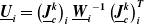 \begin{equation}\underline{\boldsymbol{U}}_{\boldsymbol{i}}=\left(\underline{\boldsymbol{J}}_{\boldsymbol{c}}^{\boldsymbol{k}}\right)_{\boldsymbol{i}}{\underline{\boldsymbol{W}}_{\boldsymbol{i}}}^{-\textbf{1}}\left(\underline{\boldsymbol{J}}_{\boldsymbol{c}}^{\boldsymbol{k}}\right)_{\boldsymbol{i}}^{\boldsymbol{T}}\end{equation}
 \begin{equation}\tilde{\boldsymbol{\lambda }}_{\boldsymbol{i}}^{{\textbf{opt}}}=-\underline{\boldsymbol{U}}_{\boldsymbol{i}}^{-\textbf{1}}\dot{\tilde{\boldsymbol{X}}}_{\boldsymbol{i}}\end{equation}
In addition, substituting $\tilde{\boldsymbol{\lambda }}_{\boldsymbol{i}}^{\boldsymbol{\textbf{opt}}}$
into Eq. (18), one can solve for the minimum norm
$\tilde{\boldsymbol{\lambda }}_{\boldsymbol{i}}^{\boldsymbol{\textbf{opt}}}$
into Eq. (18), one can solve for the minimum norm $\dot{\tilde{\boldsymbol{q}}}_{i}$
and
$\dot{\tilde{\boldsymbol{q}}}_{i}$
and $\ddot{\tilde{\boldsymbol{q}}}_{\boldsymbol{i},\boldsymbol{\min }}$
as follows:
$\ddot{\tilde{\boldsymbol{q}}}_{\boldsymbol{i},\boldsymbol{\min }}$
as follows:
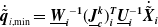 \begin{equation}\dot{\tilde{\boldsymbol{q}}}_{i,\min}={\underline{\boldsymbol{W}}_{\boldsymbol{i}}}^{-\textbf{1}}(\underline{\boldsymbol{J}}_{\boldsymbol{c}}^{\boldsymbol{k}})_{\boldsymbol{i}}^{\boldsymbol{T}}\underline{\boldsymbol{U}}_{\boldsymbol{i}}^{-\textbf{1}}\dot{\tilde{\boldsymbol{X}}}_{\boldsymbol{i}}\end{equation}
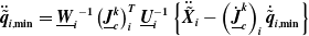 \begin{equation}\ddot{\tilde{\boldsymbol{q}}}_{\boldsymbol{i},\boldsymbol{\min }}={\underline{\boldsymbol{W}}_{\boldsymbol{i}}}^{-\textbf{1}}\left(\underline{\boldsymbol{J}}_{\boldsymbol{c}}^{\boldsymbol{k}}\right)_{\boldsymbol{i}}^{\boldsymbol{T}}\underline{\boldsymbol{U}}_{\boldsymbol{i}}^{-\textbf{1}}\left\{\ddot{\tilde{\boldsymbol{X}}}_{\boldsymbol{i}}-\left(\underline{\dot{\boldsymbol{J}}}_{\boldsymbol{c}}^{\boldsymbol{k}}\right)_{\boldsymbol{i}}\dot{\tilde{\boldsymbol{q}}}_{\boldsymbol{i},\boldsymbol{\min }}\right\}\end{equation}
Furthermore, referring to the first part of the control block diagram, the impedance control scheme can be employed to generate trajectories for the both end-effectors to track the target payload as described below:
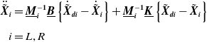 \begin{align} \ddot{\tilde{\boldsymbol{X}}}_{\boldsymbol{i}}&=\underline{\boldsymbol{M}}_{\boldsymbol{i}}^{-\textbf{1}}\underline{\boldsymbol{B}}\left\{\dot{\tilde{\boldsymbol{X}}}_{\boldsymbol{di}}-\dot{\tilde{\boldsymbol{X}}}_{\boldsymbol{i}}\right\}+\underline{\boldsymbol{M}}_{\boldsymbol{i}}^{-\textbf{1}}\underline{\boldsymbol{K}}\left\{\tilde{\boldsymbol{X}}_{\boldsymbol{di}}-\tilde{\boldsymbol{X}}_{\boldsymbol{i}}\right\} \nonumber\\[3pt]i&=L, R\end{align}
where $\underline{\boldsymbol{M}}_{\boldsymbol{i}}$ $\underline{\boldsymbol{B}}$
,
$\underline{\boldsymbol{B}}$
, $\underline{\boldsymbol{K}}$
are (6×6) positive definite matrices and are selected to satisfy the tracking performance requirements while
$\underline{\boldsymbol{K}}$
are (6×6) positive definite matrices and are selected to satisfy the tracking performance requirements while $\tilde{\boldsymbol{X}}_{\boldsymbol{di}}$
and
$\tilde{\boldsymbol{X}}_{\boldsymbol{di}}$
and $\tilde{\boldsymbol{X}}_{\boldsymbol{i}}$
are the desired payload and the end-effector trajectory respectively [Reference Kalaycioglu and de Ruiter54]. The matrix selection process will not be discussed here for the sake of brevity.
$\tilde{\boldsymbol{X}}_{\boldsymbol{i}}$
are the desired payload and the end-effector trajectory respectively [Reference Kalaycioglu and de Ruiter54]. The matrix selection process will not be discussed here for the sake of brevity.
Through the application of the inverse dynamics of the system as shown in the control block diagram, the joint torques, and the chaser spacecraft moments then can be calculated accordingly as shown below:
 \begin{equation}\left[\begin{array}{c} \tilde{\boldsymbol{F}}_{\boldsymbol{c}}\\ \\[-5pt] \tilde{\boldsymbol{\tau }}_{\boldsymbol{c}}\\ \\[-5pt] \tilde{\boldsymbol{\tau }}_{{\boldsymbol{\theta }_{\boldsymbol{L}}}}\\ \\[-5pt] \tilde{\boldsymbol{\tau }}_{{\boldsymbol{\theta }_{\boldsymbol{R}}}} \end{array}\right]=\left[\begin{array}{c@{\quad}c@{\quad}c@{\quad}c} \boldsymbol{G}_{\boldsymbol{v}} & \boldsymbol{G}_{\boldsymbol{c}\boldsymbol{\omega }} & \boldsymbol{G}_{\boldsymbol{c}{\boldsymbol{\theta }_{\boldsymbol{L}}}} & \boldsymbol{G}_{\boldsymbol{c}{\boldsymbol{\theta }_{\boldsymbol{R}}}}\\ \\[-5pt] \boldsymbol{G}_{\boldsymbol{cw}}^{\boldsymbol{T}} & \boldsymbol{G}_{\boldsymbol{w}} & \boldsymbol{G}_{{\boldsymbol{w}\boldsymbol{\theta }_{\boldsymbol{L}}}} & \boldsymbol{G}_{{\boldsymbol{w}\boldsymbol{\theta }_{\boldsymbol{R}}}}\\ \\[-5pt] \boldsymbol{G}_{\boldsymbol{c}\boldsymbol{\theta }_{\boldsymbol{L}}}^{\boldsymbol{T}} & \boldsymbol{G}_{\boldsymbol{w}\boldsymbol{\theta }_{\boldsymbol{L}}}^{\boldsymbol{T}} & \boldsymbol{G}_{{\boldsymbol{\theta }_{\boldsymbol{L}}}} & \boldsymbol{G}_{{\boldsymbol{\theta }_{\boldsymbol{LR}}}}\\ \\[-5pt] \boldsymbol{G}_{\boldsymbol{c}\boldsymbol{\theta }_{\boldsymbol{R}}}^{\boldsymbol{T}} & \boldsymbol{G}_{\boldsymbol{w}\boldsymbol{\theta }_{\boldsymbol{R}}}^{\boldsymbol{T}} & \boldsymbol{G}_{\boldsymbol{\theta }_{\boldsymbol{LR}}}^{\boldsymbol{T}} & \boldsymbol{G}_{{\boldsymbol{\theta }_{\boldsymbol{R}}}} \end{array}\right]\left[\begin{array}{c} \ddot{\tilde{\boldsymbol{R}}}_{\boldsymbol{c}}\\ \\[-5pt] \dot{\tilde{\boldsymbol{\omega }}}_{\boldsymbol{c}}\\ \\[-5pt] \ddot{\tilde{\boldsymbol{\theta }}}_{\boldsymbol{L}}\\ \\[-5pt] \ddot{\tilde{\boldsymbol{\theta }}}_{\boldsymbol{R}} \end{array}\right]+\left[\begin{array}{c} \tilde{\boldsymbol{c}}_{\boldsymbol{v}}\\ \\[-5pt] \tilde{\boldsymbol{c}}_{\boldsymbol{w}}\\ \\[-5pt] \tilde{\boldsymbol{c}}_{{\boldsymbol{\theta }_{\boldsymbol{L}}}}\\ \\[-5pt] \tilde{\boldsymbol{c}}_{{\boldsymbol{\theta }_{\boldsymbol{R}}}} \end{array}\right]\end{equation}
2.4.1.2 OCA post-capture stage
Saturation of torques of space robot joint actuators and momentum wheels mounted on a spacecraft is a major concern in real applications. In this mode of operation, a cost function $C_{p}$
is defined to minimize the joint torques
$C_{p}$
is defined to minimize the joint torques $\tilde{\boldsymbol{\tau }}_{{\boldsymbol{\theta }_{\boldsymbol{L}}}}$
,
$\tilde{\boldsymbol{\tau }}_{{\boldsymbol{\theta }_{\boldsymbol{L}}}}$
, $\tilde{\boldsymbol{\tau }}_{{\boldsymbol{\theta }_{\boldsymbol{R}}}}$
and the chaser spacecraft thrust force and moments
$\tilde{\boldsymbol{\tau }}_{{\boldsymbol{\theta }_{\boldsymbol{R}}}}$
and the chaser spacecraft thrust force and moments $\tilde{\boldsymbol{F}}_{\boldsymbol{c}}$
,
$\tilde{\boldsymbol{F}}_{\boldsymbol{c}}$
, $\tilde{\boldsymbol{\tau }}_{\boldsymbol{c}}$
and the contact forces and moments
$\tilde{\boldsymbol{\tau }}_{\boldsymbol{c}}$
and the contact forces and moments $\tilde{\boldsymbol{F}}_{\boldsymbol{i}}$
and
$\tilde{\boldsymbol{F}}_{\boldsymbol{i}}$
and $\tilde{\boldsymbol{N}}_{\boldsymbol{i}}$
applied by the robot manipulators on the target spacecraft (i.e., payload)
$\tilde{\boldsymbol{N}}_{\boldsymbol{i}}$
applied by the robot manipulators on the target spacecraft (i.e., payload)
Therefore, a cost function, $C_{p}$
can be designed as:
$C_{p}$
can be designed as:
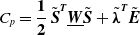 \begin{equation}C_{p}=\frac{\textbf{1}}{\textbf{2}}\,\tilde{\boldsymbol{S}}^{\boldsymbol{T} }\underline{\boldsymbol{W}}\tilde{\boldsymbol{S}}+\tilde{\boldsymbol{\lambda }}^{\boldsymbol{T}}\tilde{\boldsymbol{E}}\end{equation} $\underline{\boldsymbol{W}}$
is a square (2n + 18, 2n + 18) positive definite weighting matrix provided in Eq. (25b) while
$\underline{\boldsymbol{W}}$
is a square (2n + 18, 2n + 18) positive definite weighting matrix provided in Eq. (25b) while $\tilde{\boldsymbol{\lambda }}$
is the ((2n + 12), 1) Lagrangian multiplier and
$\tilde{\boldsymbol{\lambda }}$
is the ((2n + 12), 1) Lagrangian multiplier and $\tilde{\boldsymbol{E}}$
is a vector which consists of the constraints equations as defined by Eq. (28).
$\tilde{\boldsymbol{E}}$
is a vector which consists of the constraints equations as defined by Eq. (28).
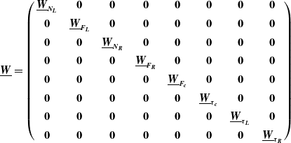 \begin{equation}\underline{\boldsymbol{W}}=\left(\begin{array}{c@{\quad}c@{\quad}c@{\quad}c@{\quad}c@{\quad}c@{\quad}c@{\quad}c} \underline{\boldsymbol{W}}_{{\boldsymbol{N}_{\boldsymbol{L}}}} & \textbf{0} & \textbf{0} & \textbf{0} & \textbf{0} & \textbf{0} & \textbf{0} & \textbf{0}\\ \\[-8pt] \textbf{0} & \underline{\boldsymbol{W}}_{{\boldsymbol{F}_{\boldsymbol{L}}}} & \textbf{0} & \textbf{0} & \textbf{0} & \textbf{0} & \textbf{0} & \textbf{0}\\ \\[-8pt] \textbf{0} & \textbf{0} & \underline{\boldsymbol{W}}_{{\boldsymbol{N}_{\boldsymbol{R}}}} & \textbf{0} & \textbf{0} & \textbf{0} & \textbf{0} & \textbf{0}\\ \\[-8pt] \textbf{0} & \textbf{0} & \textbf{0} & \underline{\boldsymbol{W}}_{{\boldsymbol{F}_{\boldsymbol{R}}}} & \textbf{0} & \textbf{0} & \textbf{0} & \textbf{0}\\ \\[-8pt] \textbf{0} & \textbf{0} & \textbf{0} & \textbf{0} & \underline{\boldsymbol{W}}_{{\boldsymbol{F}_{\boldsymbol{c}}}} & \textbf{0} & \textbf{0} & \textbf{0}\\ \\[-8pt] \textbf{0} & \textbf{0} & \textbf{0} & \textbf{0} & \textbf{0} & \underline{\boldsymbol{W}}_{{\boldsymbol{\tau }_{\boldsymbol{c}}}} & \textbf{0} & \textbf{0}\\ \\[-8pt] \textbf{0} & \textbf{0} & \textbf{0} & \textbf{0} & \textbf{0} & \textbf{0} & \underline{\boldsymbol{W}}_{{\boldsymbol{\tau }_{\boldsymbol{L}}}} & \textbf{0}\\ \\[-8pt] \textbf{0} & \textbf{0} & \textbf{0} & \textbf{0} & \textbf{0} & \textbf{0} & \textbf{0} & \underline{\boldsymbol{W}}_{{\boldsymbol{\tau }_{\boldsymbol{R}}}} \end{array}\right)\end{equation}
The $\tilde{\boldsymbol{S}}$
vector consists of the end-effector contact forces and moments as well as the chaser spacecraft control force and moments, the joint torques for the left and right arm, respectively, as given below:
$\tilde{\boldsymbol{S}}$
vector consists of the end-effector contact forces and moments as well as the chaser spacecraft control force and moments, the joint torques for the left and right arm, respectively, as given below:
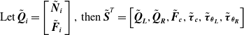 \begin{equation}\text{Let}\, \tilde{\boldsymbol{Q}}_{\boldsymbol{i}}=\left[\begin{array}{c} \tilde{\boldsymbol{N}}_{\boldsymbol{i}}\\ \\[-8pt] \tilde{\boldsymbol{F}}_{\boldsymbol{i}} \end{array}\right] , \,\textrm{then} \,\tilde{\boldsymbol{S}}^{T}=\left[\tilde{\boldsymbol{Q}}_{\boldsymbol{L}}, \tilde{\boldsymbol{Q}}_{\boldsymbol{R}},\tilde{\boldsymbol{F}}_{\boldsymbol{c}}, \tilde{\boldsymbol{\tau }}_{\boldsymbol{c}}, \tilde{\boldsymbol{\tau }}_{{\boldsymbol{\theta }_{\boldsymbol{L}}}}, \tilde{\boldsymbol{\tau }}_{{\boldsymbol{\theta }_{\boldsymbol{R}}}} \right]\end{equation}
where $\tilde{\boldsymbol{F}}_{\boldsymbol{i}}$
and
$\tilde{\boldsymbol{F}}_{\boldsymbol{i}}$
and $\tilde{\boldsymbol{N}}_{\boldsymbol{i}}$
are the contact forces and moments applied by the left and right robot manipulators on the target spacecraft, respectively, while
$\tilde{\boldsymbol{N}}_{\boldsymbol{i}}$
are the contact forces and moments applied by the left and right robot manipulators on the target spacecraft, respectively, while $\tilde{\boldsymbol{F}}_{\boldsymbol{c}}$
and
$\tilde{\boldsymbol{F}}_{\boldsymbol{c}}$
and $\tilde{\boldsymbol{\tau }}_{\boldsymbol{c}}$
are the chaser spacecraft control thrust forces and moments.
$\tilde{\boldsymbol{\tau }}_{\boldsymbol{c}}$
are the chaser spacecraft control thrust forces and moments.
The $\tilde{\boldsymbol{E}}$
vector can be calculated as follows:
$\tilde{\boldsymbol{E}}$
vector can be calculated as follows:
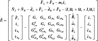 \begin{equation}\tilde{\boldsymbol{E}}=\left[\begin{array}{c} \tilde{\boldsymbol{F}}_{\boldsymbol{L}}+\tilde{\boldsymbol{F}}_{\boldsymbol{R}}-\boldsymbol{m}_{\boldsymbol{t}}\ddot{\boldsymbol{x}}_{\boldsymbol{t}}\\ \\[-8pt] \tilde{\boldsymbol{N}}_{\boldsymbol{L}}+\tilde{\boldsymbol{N}}_{\boldsymbol{R}}-\tilde{\boldsymbol{d}}_{\boldsymbol{L}}\times \tilde{\boldsymbol{F}}_{\boldsymbol{L}}-\tilde{\boldsymbol{d}}_{\boldsymbol{R}}\times \tilde{\boldsymbol{F}}_{\boldsymbol{R}}-\left[\boldsymbol{I}_{\boldsymbol{t}}\boldsymbol{\Omega }_{\boldsymbol{t}}+\boldsymbol{\Omega }_{\boldsymbol{t}}\times \boldsymbol{I}_{\boldsymbol{t}}\boldsymbol{\Omega }_{\boldsymbol{t}}\right]\\ \\[-8pt] \left[\begin{array}{c} \tilde{\boldsymbol{F}}_{\boldsymbol{c}}\\ \\[-8pt] \tilde{\boldsymbol{\tau }}_{\boldsymbol{c}}\\ \\[-8pt] \tilde{\boldsymbol{\tau }}_{{\boldsymbol{\theta }_{\boldsymbol{L}}}}\\ \\[-8pt] \tilde{\boldsymbol{\tau }}_{{\boldsymbol{\theta }_{\boldsymbol{R}}}} \end{array}\right]-\left[\begin{array}{cccc} \boldsymbol{G}_{\boldsymbol{v}} & \boldsymbol{G}_{\boldsymbol{c}\boldsymbol{\omega }} & \boldsymbol{G}_{\boldsymbol{c}{\boldsymbol{\theta }_{\boldsymbol{L}}}} & \boldsymbol{G}_{\boldsymbol{c}{\boldsymbol{\theta }_{\boldsymbol{R}}}}\\ \\[-8pt] \boldsymbol{G}_{\boldsymbol{cw}}^{\boldsymbol{T}} & \boldsymbol{G}_{\boldsymbol{w}} & \boldsymbol{G}_{{\boldsymbol{w}\boldsymbol{\theta }_{\boldsymbol{L}}}} & \boldsymbol{G}_{{\boldsymbol{w}\boldsymbol{\theta }_{\boldsymbol{R}}}}\\ \\[-8pt] \boldsymbol{G}_{\boldsymbol{c}\boldsymbol{\theta }_{\boldsymbol{L}}}^{\boldsymbol{T}} & \boldsymbol{G}_{\boldsymbol{w}\boldsymbol{\theta }_{\boldsymbol{L}}}^{\boldsymbol{T}} & \boldsymbol{G}_{{\boldsymbol{\theta }_{\boldsymbol{L}}}} & \boldsymbol{G}_{{\boldsymbol{\theta }_{\boldsymbol{LR}}}}\\ \\[-8pt] \boldsymbol{G}_{\boldsymbol{c}\boldsymbol{\theta }_{\boldsymbol{R}}}^{\boldsymbol{T}} & \boldsymbol{G}_{\boldsymbol{w}\boldsymbol{\theta }_{\boldsymbol{R}}}^{\boldsymbol{T}} & \boldsymbol{G}_{\boldsymbol{\theta }_{\boldsymbol{LR}}}^{\boldsymbol{T}} & \boldsymbol{G}_{{\boldsymbol{\theta }_{\boldsymbol{R}}}} \end{array}\right]\left[\begin{array}{c} \ddot{\tilde{\boldsymbol{R}}}_{\boldsymbol{c}}\\ \\[-8pt] \dot{\tilde{\boldsymbol{\omega }}}_{\boldsymbol{c}}\\ \\[-8pt] \ddot{\tilde{\boldsymbol{\theta }}}_{\boldsymbol{L}}\\ \\[-8pt] \ddot{\tilde{\boldsymbol{\theta }}}_{\boldsymbol{R}} \end{array}\right]-\left[\begin{array}{c} \tilde{\boldsymbol{c}}_{\boldsymbol{v}}\\ \\[-8pt] \tilde{\boldsymbol{c}}_{\boldsymbol{w}}\\ \\[-8pt] \tilde{\boldsymbol{c}}_{{\boldsymbol{\theta }_{\boldsymbol{L}}}}\\ \\[-8pt] \tilde{\boldsymbol{c}}_{{\boldsymbol{\theta }_{\boldsymbol{R}}}} \end{array}\right] \end{array}\right]\end{equation}
where $\tilde{\boldsymbol{d}}_{\boldsymbol{L}}$
,
$\tilde{\boldsymbol{d}}_{\boldsymbol{L}}$
, $\tilde{\boldsymbol{d}}_{\boldsymbol{R}}$
are the displacement vectors from the left and right end-effectors to the center of mass of the target spacecraft, respectively. Also,
$\tilde{\boldsymbol{d}}_{\boldsymbol{R}}$
are the displacement vectors from the left and right end-effectors to the center of mass of the target spacecraft, respectively. Also, $\tilde{\boldsymbol{d}}_{\boldsymbol{L}}\times$ $\tilde{\boldsymbol{F}}_{\boldsymbol{L}}$
can be re-written as a matrix multiplication as
$\tilde{\boldsymbol{F}}_{\boldsymbol{L}}$
can be re-written as a matrix multiplication as $\underline{\boldsymbol{D}}$
L
$\underline{\boldsymbol{D}}$
L $\tilde{\boldsymbol{F}}_{\boldsymbol{L}}$
, where
$\tilde{\boldsymbol{F}}_{\boldsymbol{L}}$
, where $\tilde{\boldsymbol{d}}_{\boldsymbol{L}}$
= (
$\tilde{\boldsymbol{d}}_{\boldsymbol{L}}$
= ( $x_{L}$
,
$x_{L}$
, $y_{L}$
,
$y_{L}$
, $z_{L}$
)T and then
$z_{L}$
)T and then
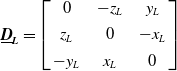 \begin{equation}\underline{\boldsymbol{D}}_{\boldsymbol{L}}=\left[\begin{array}{c@{\quad}c@{\quad}c} 0 & -z_{L} & y_{L}\\ \\[-8pt] z_{L} & 0 & -x_{L}\\ \\[-8pt] -y_{L} & x_{L} & 0 \end{array}\right]\end{equation}
and L can be replaced by R for the right robot.
The cost function $C_{p}$
can be minimized by differentiating
$C_{p}$
can be minimized by differentiating $C_{p}$
with respect to
$C_{p}$
with respect to $\tilde{\boldsymbol{\lambda }}_{\boldsymbol{i}}$
and
$\tilde{\boldsymbol{\lambda }}_{\boldsymbol{i}}$
and $\tilde{\boldsymbol{S}}$
to calculate the minimum norm of joint torques and end-effectors force and moments exerted on the target spacecraft.
$\tilde{\boldsymbol{S}}$
to calculate the minimum norm of joint torques and end-effectors force and moments exerted on the target spacecraft.
 \begin{equation}\frac{\boldsymbol\partial C_{p}}{\boldsymbol\partial \tilde{\boldsymbol{S}}}=\tilde{\textbf{0}}\end{equation}
and
 \begin{equation}\frac{\boldsymbol\partial C_{p}}{\boldsymbol\partial \tilde{\boldsymbol{\lambda }}}=\tilde{\textbf{0}}\end{equation}
Carrying out some algebraic manipulations, one can eliminate $\tilde{\boldsymbol{\lambda }}$
from the equations and obtain the minimum norm of
$\tilde{\boldsymbol{\lambda }}$
from the equations and obtain the minimum norm of $\tilde{\boldsymbol{S}}$
vector as provided in Eq. (31).
$\tilde{\boldsymbol{S}}$
vector as provided in Eq. (31).
 \begin{equation}\tilde{\boldsymbol{S}} = \underline{ \boldsymbol{\Delta }}^{-\textbf{1}}\tilde{\boldsymbol{P}}\end{equation}
where $\underline{\boldsymbol{\Delta }}$
is a ((2n + 18) × (2n + 18)) square matrix.
$\underline{\boldsymbol{\Delta }}$
is a ((2n + 18) × (2n + 18)) square matrix. $\underline{\boldsymbol{\Delta }}$
and
$\underline{\boldsymbol{\Delta }}$
and $\tilde{\boldsymbol{P}}$
are given below:
$\tilde{\boldsymbol{P}}$
are given below:
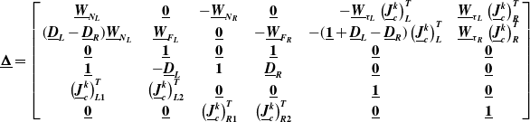 \begin{equation}\underline{\boldsymbol{\Delta }}=\left[\begin{array}{c@{\quad}c@{\quad}c@{\quad}c@{\quad}c@{\quad}c} \underline{\boldsymbol{W}}_{{\boldsymbol{N}_{\boldsymbol{L}}}} & \underline{\textbf{0}} & -\underline{\boldsymbol{W}}_{{\boldsymbol{N}_{\boldsymbol{R}}}} & \underline{\textbf{0}} & -\underline{\boldsymbol{W}}_{{\boldsymbol{\tau }_{\boldsymbol{L}}}}\left(\underline{\boldsymbol{J}}_{\boldsymbol{c}}^{\boldsymbol{k}}\right)_{\boldsymbol{L}}^{\boldsymbol{T}} & \underline{\boldsymbol{W}}_{{\boldsymbol{\tau }_{\boldsymbol{L}}}}\left(\underline{\boldsymbol{J}}_{\boldsymbol{c}}^{\boldsymbol{k}}\right)_{\boldsymbol{R}}^{\boldsymbol{T}}\\ (\underline{\boldsymbol{D}}_{\boldsymbol{L}}-\underline{\boldsymbol{D}}_{\boldsymbol{R}})\underline{\boldsymbol{W}}_{{\boldsymbol{N}_{\boldsymbol{L}}}} & \underline{\boldsymbol{W}}_{{\boldsymbol{F}_{\boldsymbol{L}}}} & \underline{\textbf{0}} & -\underline{\boldsymbol{W}}_{{\boldsymbol{F}_{\boldsymbol{R}}}} & -(\underline{\textbf{1}}+\underline{\boldsymbol{D}}_{\boldsymbol{L}}-\underline{\boldsymbol{D}}_{\boldsymbol{R}})\left(\underline{\boldsymbol{J}}_{\boldsymbol{c}}^{\boldsymbol{k}}\right)_{\boldsymbol{L}}^{\boldsymbol{T}} & \underline{\boldsymbol{W}}_{{\boldsymbol{\tau }_{\boldsymbol{R}}}}\left(\underline{\boldsymbol{J}}_{\boldsymbol{c}}^{\boldsymbol{k}}\right)_{\boldsymbol{R}}^{\boldsymbol{T}}\\ \underline{\textbf{0}} & \underline{\textbf{1}} & \underline{\textbf{0}} & \underline{\textbf{1}} & \underline{\textbf{0}} & \underline{\textbf{0}}\\ \underline{\textbf{1}} & -\underline{\boldsymbol{D}}_{\boldsymbol{L}} & \textbf{1} & \underline{\boldsymbol{D}}_{\boldsymbol{R}} & \underline{\textbf{0}} & \underline{\textbf{0}}\\ \left(\underline{\boldsymbol{J}}_{\boldsymbol{c}}^{\boldsymbol{k}}\right)_{\boldsymbol{L}\textbf{1}}^{\boldsymbol{T}} & \left(\underline{\boldsymbol{J}}_{\boldsymbol{c}}^{\boldsymbol{k}}\right)_{\boldsymbol{L}\textbf{2}}^{\boldsymbol{T}} & \underline{\textbf{0}} & \underline{\textbf{0}} & \underline{\textbf{1}} & \underline{\textbf{0}}\\ \underline{\textbf{0}} & \underline{\textbf{0}} & \left(\underline{\boldsymbol{J}}_{\boldsymbol{c}}^{\boldsymbol{k}}\right)_{\boldsymbol{R}\textbf{1}}^{\boldsymbol{T}} & \left(\underline{\boldsymbol{J}}_{\boldsymbol{c}}^{\boldsymbol{k}}\right)_{\boldsymbol{R}\textbf{2}}^{\boldsymbol{T}} & \underline{\textbf{0}} & \underline{\textbf{1}} \end{array}\right]\end{equation}
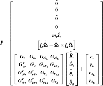 \begin{equation}\tilde{\boldsymbol{P}}=\left[\begin{array}{c} \tilde{\textbf{0}}\\ \tilde{\textbf{0}}\\ \\[-8pt] \tilde{\textbf{0}}\\ \\[-8pt] \tilde{\textbf{0}}\\ \\[-8pt] \boldsymbol{m}_{\boldsymbol{t}}\ddot{\tilde{\boldsymbol{x}}}_{\boldsymbol{t}}\\ \\[-8pt] \left[\underline{\boldsymbol{I}}_{\boldsymbol{t}}\dot{\tilde{\boldsymbol{\Omega }}}_{\boldsymbol{t}}+\tilde{\boldsymbol{\Omega }}_{\boldsymbol{t}}\times \underline{\boldsymbol{I}}_{\boldsymbol{t}}\tilde{\boldsymbol{\Omega }}_{\boldsymbol{t}}\right]\\ \\[-8pt] \left[\begin{array}{cccc} \boldsymbol{G}_{\boldsymbol{v}} & \boldsymbol{G}_{\boldsymbol{c}\boldsymbol{\omega }} & \boldsymbol{G}_{\boldsymbol{c}{\boldsymbol{\theta }_{\boldsymbol{L}}}} & \boldsymbol{G}_{\boldsymbol{c}{\boldsymbol{\theta }_{\boldsymbol{R}}}}\\ \\[-8pt] \boldsymbol{G}_{\boldsymbol{cw}}^{\boldsymbol{T}} & \boldsymbol{G}_{\boldsymbol{w}} & \boldsymbol{G}_{{\boldsymbol{w}\boldsymbol{\theta }_{\boldsymbol{L}}}} & \boldsymbol{G}_{{\boldsymbol{w}\boldsymbol{\theta }_{\boldsymbol{R}}}}\\ \\[-8pt] \boldsymbol{G}_{\boldsymbol{c}\boldsymbol{\theta }_{\boldsymbol{L}}}^{\boldsymbol{T}} & \boldsymbol{G}_{\boldsymbol{w}\boldsymbol{\theta }_{\boldsymbol{L}}}^{\boldsymbol{T}} & \boldsymbol{G}_{{\boldsymbol{\theta }_{\boldsymbol{L}}}} & \boldsymbol{G}_{{\boldsymbol{\theta }_{\boldsymbol{LR}}}}\\ \\[-8pt] \boldsymbol{G}_{\boldsymbol{c}\boldsymbol{\theta }_{\boldsymbol{R}}}^{\boldsymbol{T}} & \boldsymbol{G}_{\boldsymbol{w}\boldsymbol{\theta }_{\boldsymbol{R}}}^{\boldsymbol{T}} & \boldsymbol{G}_{\boldsymbol{\theta }_{\boldsymbol{LR}}}^{\boldsymbol{T}} & \boldsymbol{G}_{{\boldsymbol{\theta }_{\boldsymbol{R}}}} \end{array}\right]\left[\begin{array}{c} \ddot{\tilde{\boldsymbol{R}}}_{\boldsymbol{c}}\\ \\[-8pt] \dot{\tilde{\boldsymbol{\omega }}}_{\boldsymbol{c}}\\ \\[-8pt] \ddot{\tilde{\boldsymbol{\theta }}}_{\boldsymbol{L}}\\ \\[-8pt] \ddot{\tilde{\boldsymbol{\theta }}}_{\boldsymbol{R}} \end{array}\right]+\left[\begin{array}{c} \tilde{\boldsymbol{c}}_{\boldsymbol{v}}\\ \\[-8pt] \tilde{\boldsymbol{c}}_{\boldsymbol{w}}\\ \\[-8pt] \tilde{\boldsymbol{c}}_{{\boldsymbol{\theta }_{\boldsymbol{L}}}}\\ \\[-8pt] \tilde{\boldsymbol{c}}_{{\boldsymbol{\theta }_{\boldsymbol{R}}}} \end{array}\right] \end{array}\right]\end{equation}
where $\dot{\tilde{\boldsymbol{x}}}_{\boldsymbol{t}}$
and
$\dot{\tilde{\boldsymbol{x}}}_{\boldsymbol{t}}$
and $\tilde{\boldsymbol{\Omega }}_{\boldsymbol{t}}$
are the linear and rotational velocity of the center of mass of the payload,
$\tilde{\boldsymbol{\Omega }}_{\boldsymbol{t}}$
are the linear and rotational velocity of the center of mass of the payload,
 \begin{equation}\dot{\tilde{\boldsymbol{X}}}_{\boldsymbol{di}} = \left[\begin{array}{c} \tilde{\boldsymbol{\Omega }}_{\boldsymbol{t}}\\ \\[-8pt] \dot{\tilde{\boldsymbol{x}}}_{\boldsymbol{t}} \end{array}\right]\end{equation}
where $\underline{\boldsymbol{W}}_{\boldsymbol{Ni}}$
and
$\underline{\boldsymbol{W}}_{\boldsymbol{Ni}}$
and $\underline{\boldsymbol{W}}_{\boldsymbol{\tau }\boldsymbol{i}}$
are the sub-weighting matrices, and they are the components of the
$\underline{\boldsymbol{W}}_{\boldsymbol{\tau }\boldsymbol{i}}$
are the sub-weighting matrices, and they are the components of the $\underline{\boldsymbol{W}}$
square (2n + 18, 2n + 18) weighting matrix while
$\underline{\boldsymbol{W}}$
square (2n + 18, 2n + 18) weighting matrix while $(\underline{\boldsymbol{J}}_{\boldsymbol{c}}^{\boldsymbol{k}})_{\boldsymbol{L}\textbf{1}}^{\boldsymbol{T}}$
and
$(\underline{\boldsymbol{J}}_{\boldsymbol{c}}^{\boldsymbol{k}})_{\boldsymbol{L}\textbf{1}}^{\boldsymbol{T}}$
and $(\underline{\boldsymbol{J}}_{\boldsymbol{c}}^{\boldsymbol{k}})_{\boldsymbol{R}\textbf{1}}^{\boldsymbol{T}}$
are (n × 3) partial Jacobian matrices defined as below:
$(\underline{\boldsymbol{J}}_{\boldsymbol{c}}^{\boldsymbol{k}})_{\boldsymbol{R}\textbf{1}}^{\boldsymbol{T}}$
are (n × 3) partial Jacobian matrices defined as below:
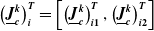 \begin{equation}\left(\underline{\boldsymbol{J}}_{\boldsymbol{c}}^{\boldsymbol{k}}\right)_{\boldsymbol{i}}^{\boldsymbol{T}}=\left[\left(\underline{\boldsymbol{J}}_{\boldsymbol{c}}^{\boldsymbol{k}}\right)_{\boldsymbol{i}\textbf{1}}^{\boldsymbol{T}}, \left(\underline{\boldsymbol{J}}_{\boldsymbol{c}}^{\boldsymbol{k}}\right)_{\boldsymbol{i}\textbf{2}}^{\boldsymbol{T}} \right]\end{equation}
2.4.2 The NMPC formulation
The NMPC block diagram is provided in Fig. 2(b). The NMPC block diagram simply replaces the second stage of Fig. 2(a). The reference trajectory (shown in Fig. 2(b)) is the output of the first stage, that is, the impedance control trajectory generation in Fig. 2(a). However, the future state estimates are also incorporated in the calculations to estimate the future reference trajectory values over the prediction horizon. In this case, a performance index (i.e., a cost function) of the system is optimized by implementing a robust NMPC that takes into account the predictions of the output signal and the constraints on the states, inputs, and outputs as shown in Fig. 2(b).
The main difference between the NMPC and the OCA is that the former uses a system model to predict and control the future behavior while the latter only considers the current and the past behaviors.
The NMPC algorithm is used to predict and control the system’s future behavior by implementing a set of optimization problems at each control interval. These problems are usually related to the constraints and cost functions. The cost function is a scalar that must be minimized at each interval to measure the performance of the system. In addition to the cost functions, the system can also be subjected to physical constraints on the states and plant output to check its performance. The modified states are adjusted according to the constraints applied to the system.
The conventional MPC formulation for the dual arm non-linear system can be written as:
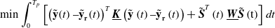 \begin{equation*} \min \int _{0}^{T_{p}}\left[ \left(\tilde{\textbf{y}}\!\left(t\right)\hbox{--}\tilde{\textbf{y}}_{\textbf{r}}\!\left(t\right)\right)^{T} \underline{\boldsymbol{K}}\left(\tilde{\textbf{y}}\left(t\right)\hbox{--}\tilde{\textbf{y}}_{\textbf{r}}\left(t\right)\right)+\tilde{\boldsymbol{S}}^{T}\left(t\right)\underline{\boldsymbol{W}}\tilde{\boldsymbol{S}}\left(\textrm{t}\right)\right] dt \end{equation*}
subject to:
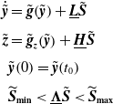 \begin{align} \dot{\tilde{\boldsymbol{y}}}& =\tilde{\boldsymbol{g}}\!\left(\tilde{\boldsymbol{y}}\right)+\underline{\boldsymbol{L}}\tilde{\boldsymbol{S}} \nonumber\\[3pt] \tilde{\boldsymbol{z}}& =\tilde{\boldsymbol{g}}_{\boldsymbol{z}}\!\left(\tilde{\boldsymbol{y}}\right)+\underline{\boldsymbol{H}}\tilde{\boldsymbol{S}} \nonumber\\[3pt]&\tilde{\boldsymbol{y}}\!\left(0\right)=\tilde{\boldsymbol{y}}\!\left(t_{0}\right) \nonumber\\[3pt]&\widetilde{ \boldsymbol{S}}_{\boldsymbol{\min }}\lt \underline{\boldsymbol{\Lambda }}\tilde{\boldsymbol{S}}\lt \widetilde{ \boldsymbol{S}}_{\boldsymbol{\max }}\end{align}
where $T_{p}$
is the prediction horizon;
$T_{p}$
is the prediction horizon; $\underline{\boldsymbol{K}}$
and
$\underline{\boldsymbol{K}}$
and $\underline{\boldsymbol{W}}$
are (2(6 + 2n)× 2(6 + 2n)) and ((18 + 2n) × (18 + 2n)) positive definite square weighting matrices, respectively;
$\underline{\boldsymbol{W}}$
are (2(6 + 2n)× 2(6 + 2n)) and ((18 + 2n) × (18 + 2n)) positive definite square weighting matrices, respectively; $\tilde{\boldsymbol{g}}(\tilde{\boldsymbol{y}}), \tilde{\boldsymbol{g}}_{\boldsymbol{z}}(\tilde{\boldsymbol{y}}), \underline{\boldsymbol{L}}, \underline{\boldsymbol{H}}$
are part of the non-linear system equations and
$\tilde{\boldsymbol{g}}(\tilde{\boldsymbol{y}}), \tilde{\boldsymbol{g}}_{\boldsymbol{z}}(\tilde{\boldsymbol{y}}), \underline{\boldsymbol{L}}, \underline{\boldsymbol{H}}$
are part of the non-linear system equations and $\underline{\boldsymbol{\Lambda }}$ $\text{is a square positive definite }\text{scaling matrix for saturation limits}$
.
$\text{is a square positive definite }\text{scaling matrix for saturation limits}$
. $\tilde{\boldsymbol{y}}({t})^{\boldsymbol{T}}=[\tilde{\boldsymbol{R}}_{\boldsymbol{c}}, \tilde{\boldsymbol{\theta }}_{\boldsymbol{L}},\tilde{\boldsymbol{\theta }}_{\boldsymbol{R}}, \dot{\tilde{\boldsymbol{R}}}_{\boldsymbol{c}}, \dot{\varphi }$
,
$\tilde{\boldsymbol{y}}({t})^{\boldsymbol{T}}=[\tilde{\boldsymbol{R}}_{\boldsymbol{c}}, \tilde{\boldsymbol{\theta }}_{\boldsymbol{L}},\tilde{\boldsymbol{\theta }}_{\boldsymbol{R}}, \dot{\tilde{\boldsymbol{R}}}_{\boldsymbol{c}}, \dot{\varphi }$
, $\dot{\psi }$
,
$\dot{\psi }$
, $\dot{\theta }, \dot{\tilde{\boldsymbol{\theta }}}_{\boldsymbol{L}}$
,
$\dot{\theta }, \dot{\tilde{\boldsymbol{\theta }}}_{\boldsymbol{L}}$
, $\dot{\tilde{\boldsymbol{\theta }}}_{\boldsymbol{R}}$
] is a (1 × 2(6 + 2n)) state vector including the chaser spacecraft position, Euler angles, and the joint angles for the left and the right arms and their rates;
$\dot{\tilde{\boldsymbol{\theta }}}_{\boldsymbol{R}}$
] is a (1 × 2(6 + 2n)) state vector including the chaser spacecraft position, Euler angles, and the joint angles for the left and the right arms and their rates; $\tilde{\boldsymbol{y}}_{\boldsymbol{r}}(\textrm{t})$
is the reference/desired states, the
$\tilde{\boldsymbol{y}}_{\boldsymbol{r}}(\textrm{t})$
is the reference/desired states, the $\tilde{\boldsymbol{S}}$
vector consists of the contact forces and moments as well as the chaser spacecraft control force and moments, the joint torques for the left and right arm, respectively, as previously defined in Eq. (26),
$\tilde{\boldsymbol{S}}$
vector consists of the contact forces and moments as well as the chaser spacecraft control force and moments, the joint torques for the left and right arm, respectively, as previously defined in Eq. (26), $\tilde{\boldsymbol{S}}^{T}=[\tilde{\boldsymbol{Q}}_{\boldsymbol{L}}, \tilde{\boldsymbol{Q}}_{\boldsymbol{R}},\tilde{\boldsymbol{F}}_{\boldsymbol{c}}, \tilde{\boldsymbol{\tau }}_{\boldsymbol{c}}, \tilde{\boldsymbol{\tau }}_{{\boldsymbol{\theta }_{\boldsymbol{L}}}}, \tilde{\boldsymbol{\tau }}_{{\boldsymbol{\theta }_{\boldsymbol{R}}}} ]$
and is constrained between
$\tilde{\boldsymbol{S}}^{T}=[\tilde{\boldsymbol{Q}}_{\boldsymbol{L}}, \tilde{\boldsymbol{Q}}_{\boldsymbol{R}},\tilde{\boldsymbol{F}}_{\boldsymbol{c}}, \tilde{\boldsymbol{\tau }}_{\boldsymbol{c}}, \tilde{\boldsymbol{\tau }}_{{\boldsymbol{\theta }_{\boldsymbol{L}}}}, \tilde{\boldsymbol{\tau }}_{{\boldsymbol{\theta }_{\boldsymbol{R}}}} ]$
and is constrained between $\widetilde{ \boldsymbol{S}}_{\boldsymbol{\min }}\text{ and}$ $\widetilde{ \boldsymbol{S}}_{\boldsymbol{\max }}$
.
$\widetilde{ \boldsymbol{S}}_{\boldsymbol{\max }}$
.
The non-linear system can now be described with an exact quasi-linear parameter varying realization [Reference Englert, a. Volz, Rhein and Graichen43].
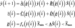 \begin{align}\tilde{\boldsymbol{y}}\!\left(\acute{k}+1\right)&=\underline{\hat{\boldsymbol{A}}}\!\left(\hat{\boldsymbol{g}}\!\left(\acute{k}\right)\right)\tilde{\boldsymbol{y}}\!\left(\acute{k}\right)+\underline{\hat{\boldsymbol{B}}}\!\left(\hat{\boldsymbol{g}}\!\left(\acute{k}\right)\right)\tilde{\boldsymbol{S}}\!\left(\acute{k}\right) \nonumber\\[3pt]\tilde{\boldsymbol{z}}\!\left(\acute{k}\right)&=\underline{\hat{\boldsymbol{C}}}\!\left(\hat{\boldsymbol{g}}\!\left(\acute{k}\right)\right)\tilde{\boldsymbol{y}}\!\left(\acute{k}\right)+\underline{\hat{\boldsymbol{D}}}\!\left(\hat{\boldsymbol{g}}\!\left(\acute{k}\right)\right)\tilde{\boldsymbol{S}}\!\left(\acute{k}\right) \\[3pt]\hat{\boldsymbol{g}}\!\left(\acute{k}\right)&=\boldsymbol{f}_{\boldsymbol{g}}\!\left(\tilde{\boldsymbol{y}}\!\left(\acute{k}\right)\right)\widetilde{ \boldsymbol{S}}_{\boldsymbol{\min }}\lt \underline{\boldsymbol{\Lambda }}\tilde{\boldsymbol{S}}\!\left(\acute{k}\right)\lt \widetilde{ \boldsymbol{S}}_{\boldsymbol{\max }}\nonumber\end{align}
where $\acute{k}$
is the sampling instant and
$\acute{k}$
is the sampling instant and $\tilde{\boldsymbol{z}}(\acute{k})$
is a vector of the measured outputs at instant
$\tilde{\boldsymbol{z}}(\acute{k})$
is a vector of the measured outputs at instant $\acute{k}$
.
$\acute{k}$
.
The NMPC is applied at each sampling instant, and the discrete states $\tilde{\boldsymbol{y}}(\acute{k})$
and control inputs
$\tilde{\boldsymbol{y}}(\acute{k})$
and control inputs $\tilde{\boldsymbol{S}}(\acute{k})$
are obtained minimizing the following performance index, that is, the Cost Function:
$\tilde{\boldsymbol{S}}(\acute{k})$
are obtained minimizing the following performance index, that is, the Cost Function:
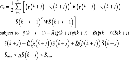 \begin{align}&C_{n}=\frac{1}{2}\sum _{j=1}^{N_{P}}\left[ \left(\tilde{\boldsymbol{y}}\!\left(\acute{k}+j\right){-}\tilde{\boldsymbol{y}}_{\boldsymbol{r}}\!\left(\acute{k}+j\right)\right)^{T} \underline{\boldsymbol{K}}\!\left(\tilde{\boldsymbol{y}}\!\left(\acute{k}+j\right){-}\tilde{\boldsymbol{y}}_{\boldsymbol{r}}\!\left(\acute{k}+j\right)\right)\right.\nonumber\\ &\qquad \left.+\,\tilde{\boldsymbol{S}}\!\left(\acute{k}+j-1\right)^{T} \underline{\boldsymbol{W}}\tilde{\boldsymbol{S}}\!\left(\acute{k}+j-1\right)\right]\nonumber\\ &\text{subject to}\quad\tilde{\boldsymbol{y}}(\acute{k}+j+1)=\underline{\hat{\boldsymbol{A}}}(\hat{\boldsymbol{g}}(\acute{k}+j))\tilde{\boldsymbol{y}}(\acute{k}+j)+\underline{\hat{\boldsymbol{B}}}(\hat{\boldsymbol{g}}(\acute{k}+j)) \tilde{\boldsymbol{S}}(\acute{k}+j) \\[3pt]&\quad \tilde{\boldsymbol{z}}\!\left(\acute{k}+j\right)=\underline{\hat{\boldsymbol{C}}}\!\left(\hat{\boldsymbol{g}}\!\left(\acute{k}+j\right)\right)\tilde{\boldsymbol{y}}\!\left(\acute{k}+j\right)+\underline{\hat{\boldsymbol{D}}}\!\left(\hat{\boldsymbol{g}}\!\left(\acute{k}+j\right)\right) \tilde{\boldsymbol{S}}\!\left(\acute{k}+j\right) \nonumber\\[3pt]&\quad \tilde{\boldsymbol{S}}_{\boldsymbol{\min }}\leq \underline{\boldsymbol{\Lambda }}\tilde{\boldsymbol{S}}\!\left(\acute{k}+j\right)\leq \tilde{\boldsymbol{S}}_{\boldsymbol{\max }}\nonumber\end{align}
The cost function $C_{n}$
can be further simplified with the substitution of
$C_{n}$
can be further simplified with the substitution of $\tilde{\boldsymbol{y}}(\acute{k}+j)$
as follows:
$\tilde{\boldsymbol{y}}(\acute{k}+j)$
as follows:
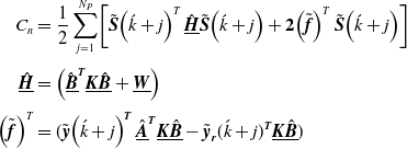 \begin{align}C_{n} & =\frac{1}{2}\sum _{j=1}^{N_{P}}\!\left[ \tilde{\boldsymbol{S}}\!\left(\acute{k}+j\right)^{T} \underline{\hat{\boldsymbol{H}}}\tilde{\boldsymbol{S}}\!\left(\acute{k}+j\right)+\textbf{2}\!\left(\tilde{\boldsymbol{f}}\right)^{T}\tilde{\boldsymbol{S}}\!\left(\acute{k}+j\right)\right] \nonumber\\[3pt]\underline{\hat{\boldsymbol{H}}} & =\left(\underline{\hat{\boldsymbol{B}}}^{\boldsymbol{T}} \underline{\boldsymbol{K}}\underline{\hat{\boldsymbol{B}}}+\underline{\boldsymbol{W}}\right) \\[3pt]\left(\tilde{\boldsymbol{f}}\right)^{T} & =(\tilde{\boldsymbol{y}}\!\left(\acute{k}+j\right)^{\boldsymbol{T}} \underline{\hat{\boldsymbol{A}}}^{\boldsymbol{T}}\underline{\boldsymbol{K}}\underline{\hat{\boldsymbol{B}}}-{\tilde{\boldsymbol{y}}_{\boldsymbol{r}}}(\acute{k}+j)^{\boldsymbol{T}}\underline{\boldsymbol{K}}\underline{\hat{\boldsymbol{B}}})\nonumber\end{align}
The cost function $C_{n}$
can be minimized by differentiating
$C_{n}$
can be minimized by differentiating $C_{n}$
with respect to
$C_{n}$
with respect to $\tilde{\boldsymbol{S}}(\acute{k}+j)$
to calculate the minimum norm of vector
$\tilde{\boldsymbol{S}}(\acute{k}+j)$
to calculate the minimum norm of vector $\tilde{\boldsymbol{S}}(\acute{k}+j)$
which consists of joint torques and end-effectors force and moments exerted on the target spacecraft.
$\tilde{\boldsymbol{S}}(\acute{k}+j)$
which consists of joint torques and end-effectors force and moments exerted on the target spacecraft.
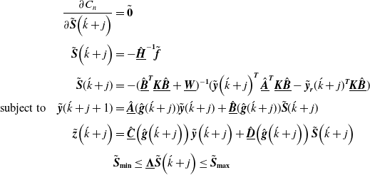 \begin{align}\frac{\partial C_{n}}{\partial \tilde{\boldsymbol{S}}\!\left(\acute{k}+j\right)}&=\tilde{\textbf{0}} \nonumber\\[3pt]\tilde{\boldsymbol{S}}\!\left(\acute{k}+j\right)&=-\underline{\hat{\boldsymbol{H}}}^{-\textbf{1}}\tilde{\boldsymbol{f}} \nonumber\\[3pt]\tilde{\boldsymbol{S}}(\acute{k}+j)&=-({\underline{\hat{\boldsymbol{B}}}^{\boldsymbol{T}}} \underline{\boldsymbol{K}}\underline{\hat{\boldsymbol{B}}}+\underline{\boldsymbol{W}})^{-\textbf{1}}(\tilde{\boldsymbol{y}}\!\left(\acute{k}+j\right)^{\boldsymbol{T}} \underline{\hat{\boldsymbol{A}}}^{\boldsymbol{T}}\underline{\boldsymbol{K}}\underline{\hat{\boldsymbol{B}}}-{\tilde{\boldsymbol{y}}_{\boldsymbol{r}}}(\acute{k}+j)^{\boldsymbol{T}}\underline{\boldsymbol{K}}\underline{\hat{\boldsymbol{B}}})\\\text{subject to}\quad \tilde{\boldsymbol{y}}(\acute{k}+j+1)&=\underline{\hat{\boldsymbol{A}}}(\hat{\boldsymbol{g}}(\acute{k}+j))\tilde{\boldsymbol{y}}(\acute{k}+j)+\underline{\hat{\boldsymbol{B}}}(\hat{\boldsymbol{g}}(\acute{k}+j)) \tilde{\boldsymbol{S}}(\acute{k}+j)\nonumber\\[3pt]\tilde{\boldsymbol{z}}\!\left(\acute{k}+j\right)&=\underline{\hat{\boldsymbol{C}}}\!\left(\hat{\boldsymbol{g}}\!\left(\acute{k}+j\right)\right)\tilde{\boldsymbol{y}}\!\left(\acute{k}+j\right)+\underline{\hat{\boldsymbol{D}}}\!\left(\hat{\boldsymbol{g}}\!\left(\acute{k}+j\right)\right) \tilde{\boldsymbol{S}}\!\left(\acute{k}+j\right) \nonumber\\[3pt]&\tilde{\boldsymbol{S}}_{\boldsymbol{\min }}\leq \underline{\boldsymbol{\Lambda }}\tilde{\boldsymbol{S}}\!\left(\acute{k}+j\right)\leq \tilde{\boldsymbol{S}}_{\boldsymbol{\max }} \nonumber\end{align}
3. Results and discussion
The computer simulation results are provided and discussed in this section. There are two sets of simulation results associated with the two modes of operation, namely pre-contact and post-capture. As noted in the literature, the challenges associated with the joint torque saturation are related to the post-capture mode; therefore, comparative simulation results for the OCA and NMPC algorithms are presented, compared, and discussed during the post-capture stage.
3.1. Pre-contact mode of operation
In this simulation, first a trajectory for the center of mass of a fictitious target spacecraft is prescribed starting from an initial condition $\tilde{\boldsymbol{x}}_{\boldsymbol{t}}^{\boldsymbol{T}}(t_{o})=[1.5,0,0,0,0,0]$
to the final condition
$\tilde{\boldsymbol{x}}_{\boldsymbol{t}}^{\boldsymbol{T}}(t_{o})=[1.5,0,0,0,0,0]$
to the final condition $\tilde{\boldsymbol{x}}_{\boldsymbol{t}}^{\boldsymbol{T}}(t_{f})=[2,0.5,0,0,0,\pi /12]$
where
$\tilde{\boldsymbol{x}}_{\boldsymbol{t}}^{\boldsymbol{T}}(t_{f})=[2,0.5,0,0,0,\pi /12]$
where $t_{o}=0$
and
$t_{o}=0$
and $t_{f}=2.5\,s$
, the initial and the final time values, respectively.
$t_{f}=2.5\,s$
, the initial and the final time values, respectively. $x_{t}^{T}$
consists of three position and three orientation angles measured in meters and radians, respectively. It is assumed that the target spacecraft is equipped with two grapple fixtures located opposite sides of the target spacecraft, and the end-effectors will track these fixtures during the pre-contact phase and eventually lock into them during the capture phase.
$x_{t}^{T}$
consists of three position and three orientation angles measured in meters and radians, respectively. It is assumed that the target spacecraft is equipped with two grapple fixtures located opposite sides of the target spacecraft, and the end-effectors will track these fixtures during the pre-contact phase and eventually lock into them during the capture phase.
The trajectories $\tilde{\boldsymbol{X}}_{\boldsymbol{di}}$
for these grapple fixtures are then calculated using the rigid body motion of the target spacecraft center of mass
$\tilde{\boldsymbol{X}}_{\boldsymbol{di}}$
for these grapple fixtures are then calculated using the rigid body motion of the target spacecraft center of mass $\tilde{\boldsymbol{x}}_{\boldsymbol{t}}^{\boldsymbol{T}}$
and the known geometry of these locations from the center of mass. Then, Eq. (23) is employed using the first stage of the control block diagram, basically the impedance control as previously presented in Fig. 2(a).
$\tilde{\boldsymbol{x}}_{\boldsymbol{t}}^{\boldsymbol{T}}$
and the known geometry of these locations from the center of mass. Then, Eq. (23) is employed using the first stage of the control block diagram, basically the impedance control as previously presented in Fig. 2(a).
The main objective of this simulation is to obtain the minimum norm of the joint angular rates for the robot manipulators while their end-effectors track the desired grapple fixture trajectories on the target spacecraft. The conventional inverse kinematics functions cannot directly be applied, and thus, the desired joint values and rates cannot uniquely be calculated since the system consists of redundant manipulators, that is, n > 6. The desired trajectories for the end-effectors were generated in the orbital plane as shown in Fig. 3(a–f).
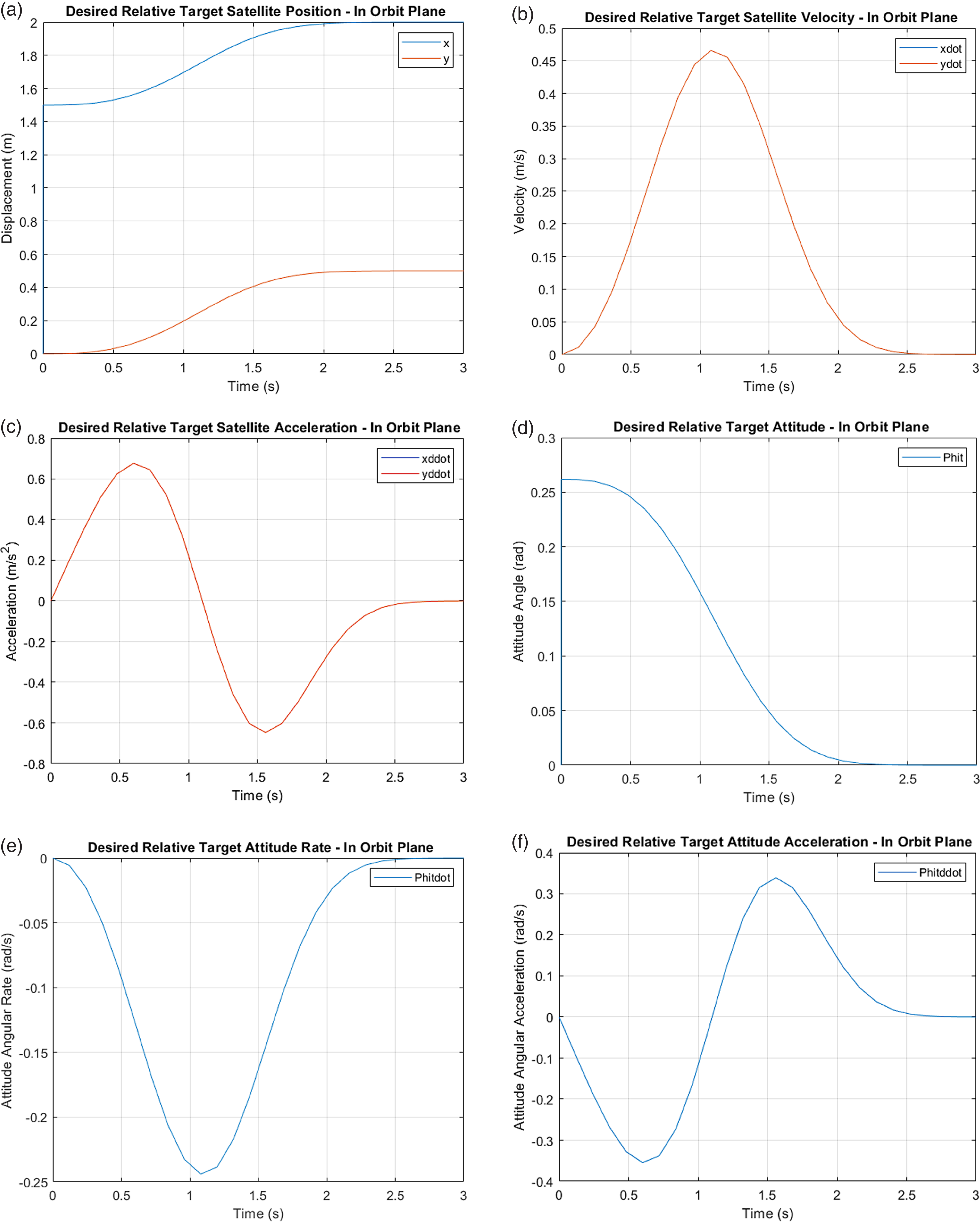
Figure 3. (a–f) Target linear and rotational displacement, velocity, and acceleration with time.
The variation of minimum norm joint rates for the left and the right arms with time is plotted in Fig. 4(a–b)
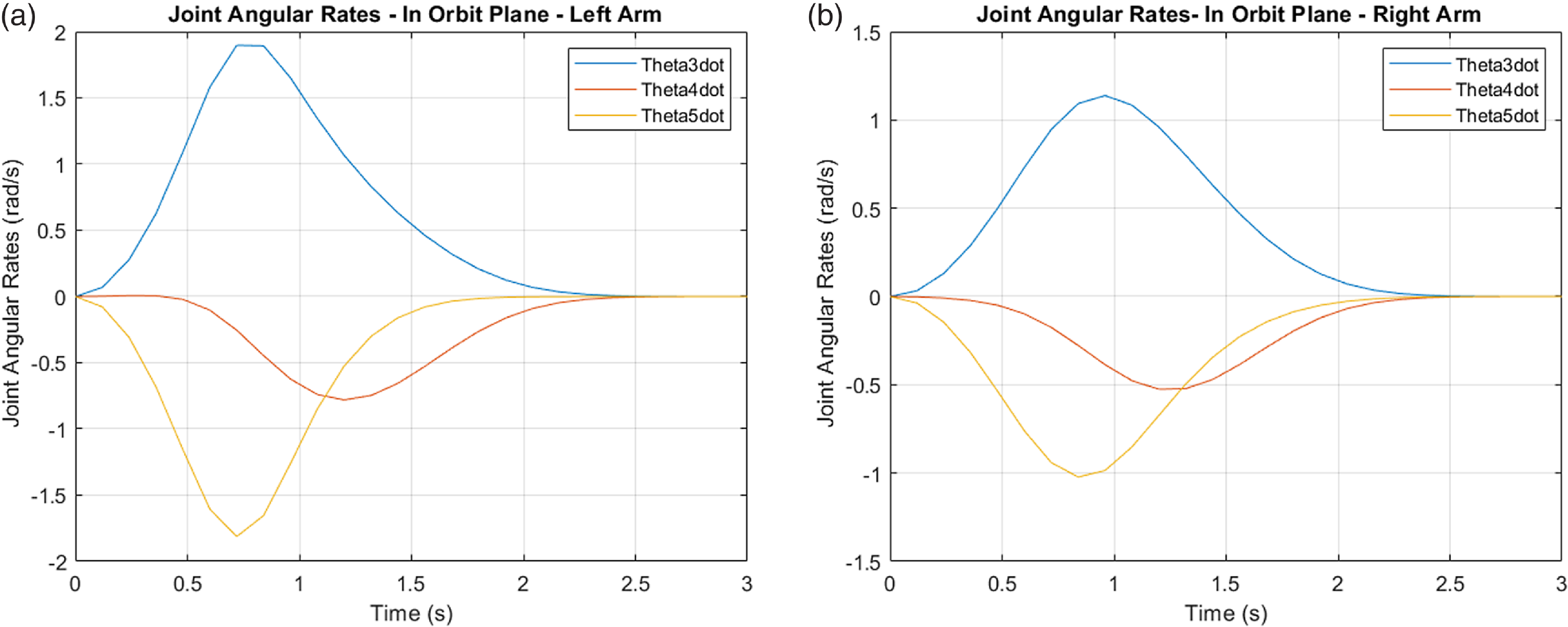
Figure 4. (a–b) Minimum norm of left and right arm joint rates.
The joint angles are obtained by integrating the joint rates using Eq. (21) and plotted in Fig. 5(a–b).
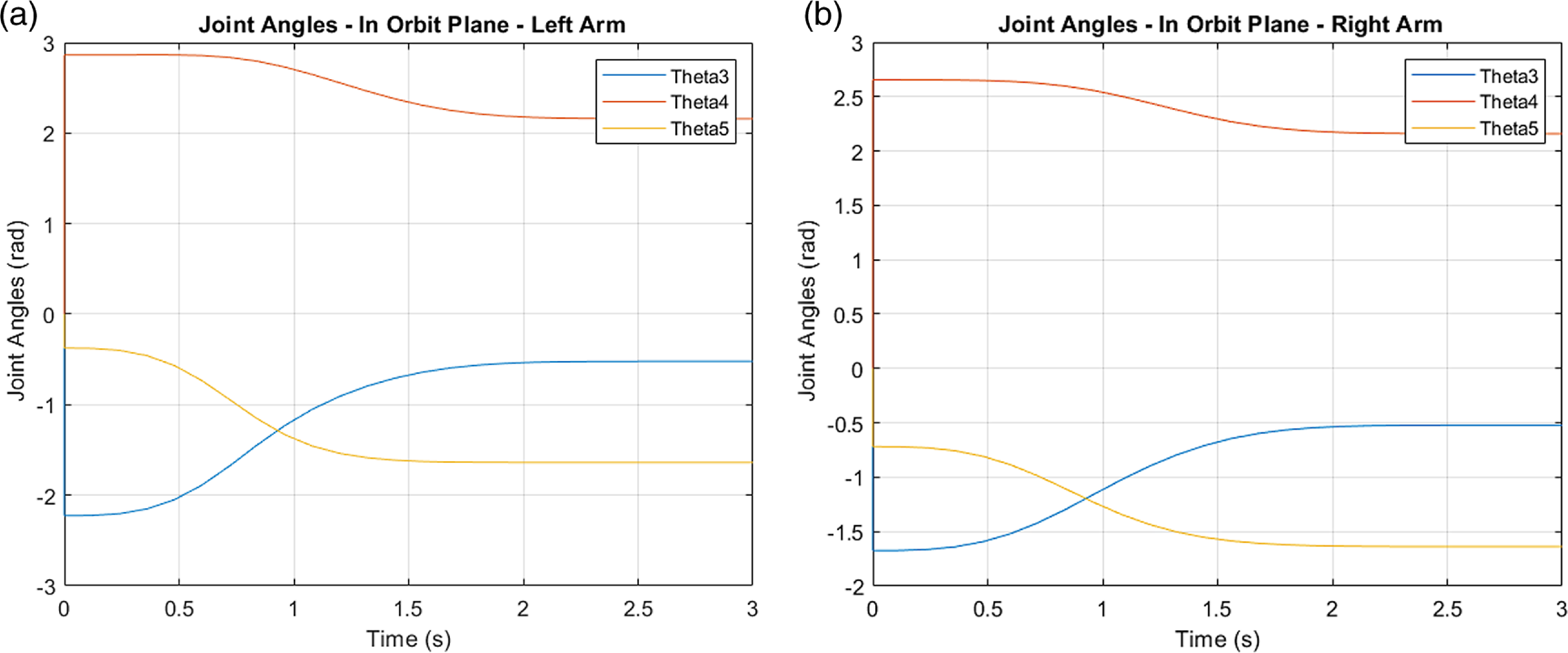
Figure 5. (a–b) Variation of optimal joint angles for left and right arms.
The joint accelerations for each robot are also calculated using Eq. (22) and are plotted with time in Fig. 6(a–b).
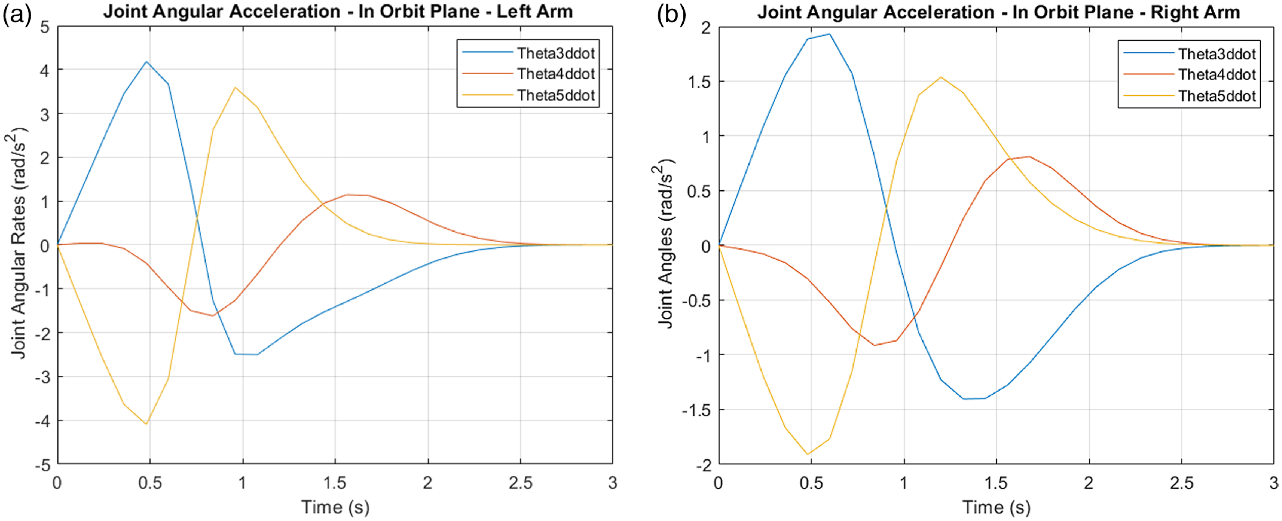
Figure 6. (a–b) Variation of optimal in-orbit joint angular accelerations for left and right arms.
The chaser spacecraft control force $\tilde{\boldsymbol{F}}_{\boldsymbol{c}}$
and moments
$\tilde{\boldsymbol{F}}_{\boldsymbol{c}}$
and moments $\tilde{\boldsymbol{\tau }}_{\boldsymbol{c}}$
are also calculated using the inverse dynamics equations as previously developed in Eq. (11) and are plotted in Fig. 7(a–b) below. These are the forces and moments transferred from the two robots to the chaser spacecraft due to the inertial angular and linear accelerations of the links.
$\tilde{\boldsymbol{\tau }}_{\boldsymbol{c}}$
are also calculated using the inverse dynamics equations as previously developed in Eq. (11) and are plotted in Fig. 7(a–b) below. These are the forces and moments transferred from the two robots to the chaser spacecraft due to the inertial angular and linear accelerations of the links.
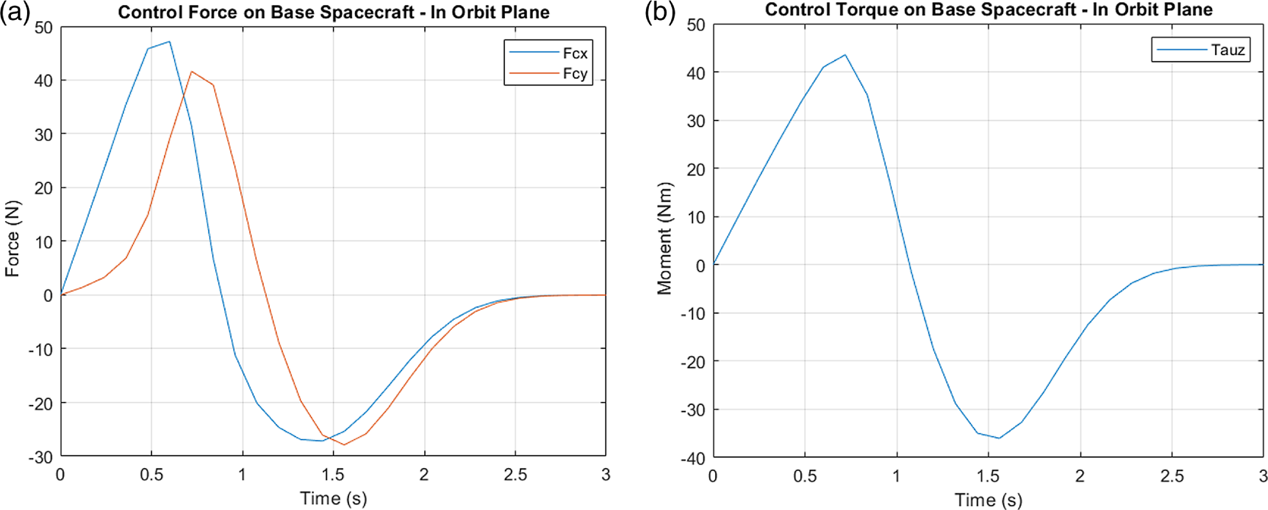
Figure 7. (a–b) Variation of chaser spacecraft control force and moments.
3.2. Post-capture mode of operation using OCA and NMPC
In this simulation, the desired trajectory for the center of mass of the target spacecraft was generated and in turn the trajectories for the left and right end-effectors were obtained while they were holding a common payload (i.e., the target spacecraft). Again, the impedance control technique as illustrated in the first stage of the control block diagram was employed for the trajectory generation. The main objective in this simulation is to obtain the minimum norm of the joint torques and chaser spacecraft control moments and forces, as well as the contact forces and moments exerted on the payload by the two robot manipulators while tracking a desired end-effector pose using both OCA and NMPC algorithms and perform a comparative analysis and discuss the relative merits of these two approaches. The desired trajectories for the end-effectors are shown in the orbital plane as shown in Fig. 8(a–f).
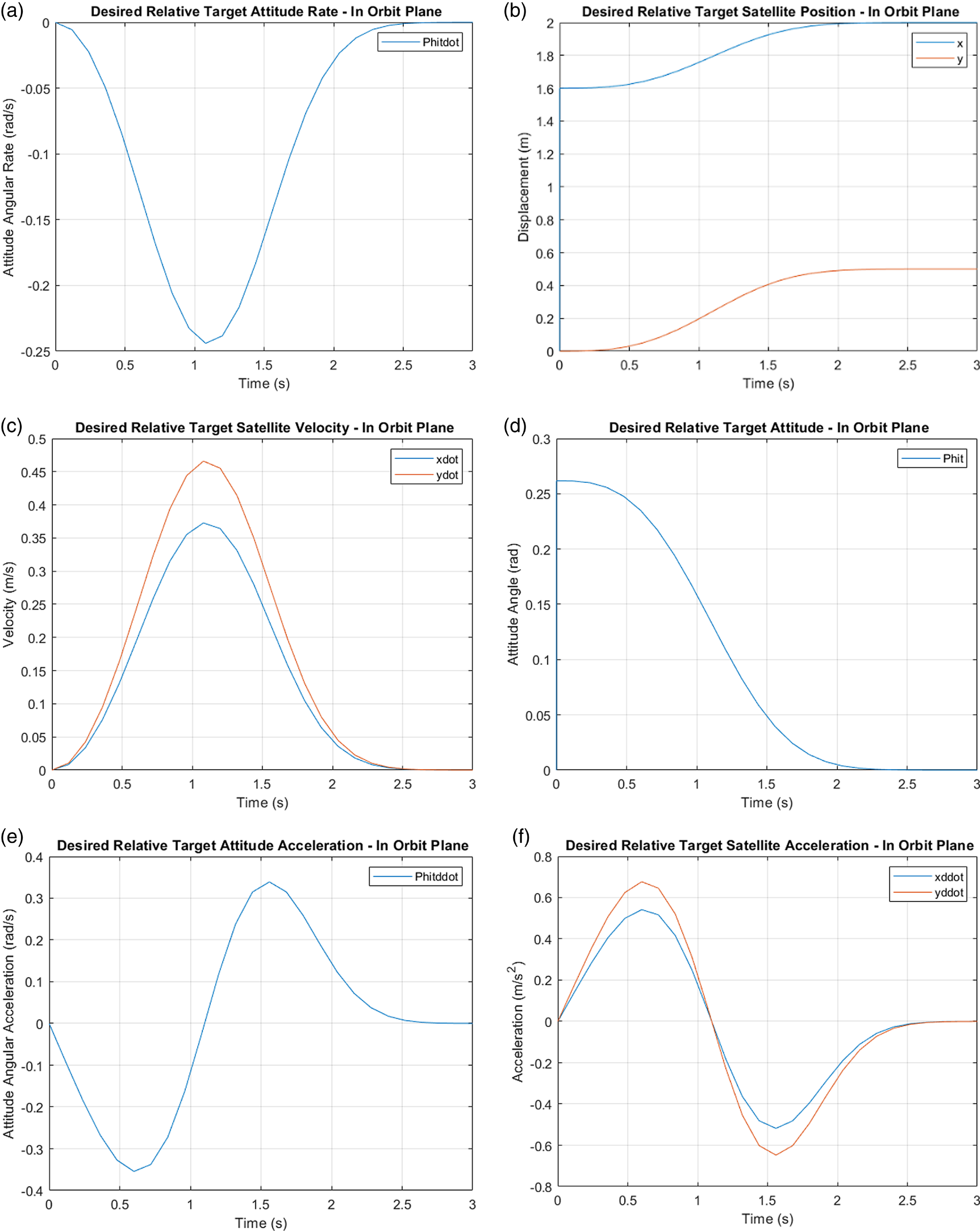
Figure 8. (a–f) Target linear and rotational displacement, velocity, and acceleration with time.
The minimum norm of the joint torques and the contact forces and moments exerted on the payload by the two robot manipulators while tracking a desired end-effector pose were plotted in Fig. 9(a–i) below using both OCA and NMPC techniques. The minimum norm in-orbit plane joint torques obtained by OCA (red lines) and NMPC (yellow lines) are plotted against the in-orbit joint torques (blue lines) obtained by only minimizing the joint rates for comparison purposes.
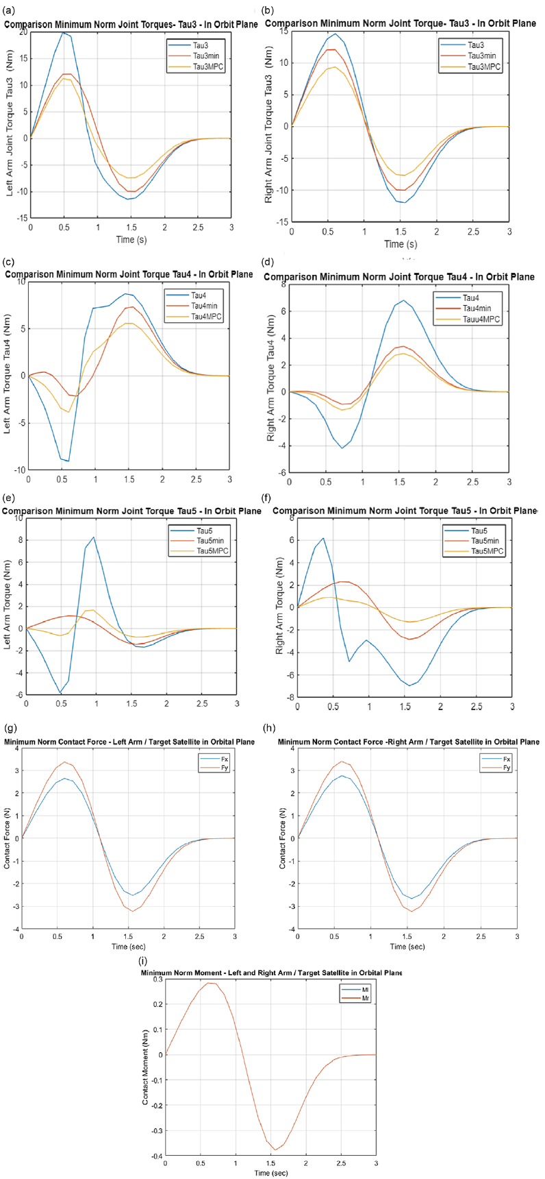
Figure 9. (a–i) Minimum joint torques (left and right arms) and the contact forces/moments.
The comparison of the joint torques clearly demonstrates that the minimization scheme by the NMPC algorithm provides the best results (i.e., the lowest joint torques, followed by the OCA and then the conventional least-square technique which is commonly used in the literature).
The NMPC approach does better in minimizing the joint torques although following a slightly different trajectory, yet arriving at the same desired destination pose. One of the reasons for this is that the performance index (i.e., the cost function) defined in Eq. (38) involves the future state estimates as well as the control inputs, and the minimization process involves not only the current state errors and current joint torques but also the future state values, and joint torques over a specified prediction horizon/future timeline. The OCA solution can be deemed as a subset solution if the prediction horizon is only assigned to the current time. Furthermore, the NMPC is a natural progression from the OCA and can be employed depending on the availability of the on-board space computing resources.
The computational complexity of the NMPC is higher than that of OCA. Especially, if one wants to use a continuous model for the NMPC estimates. This was one of the main reasons as to why the literature to date mostly focused on linear models. However, the dual arm coordination is highly non-linear, and thus, there is no MPC application on dual arm coordination. The proposed discretized technique offers exact realizations (of a non-linear model) with elegance and simplicity and yet takes into account the full non-linear model of the dual arm coordinating system as demonstrated in the simulations.
The chaser-base spacecraft control force $\tilde{\boldsymbol{F}}_{\boldsymbol{c}}$
and moments
$\tilde{\boldsymbol{F}}_{\boldsymbol{c}}$
and moments $\tilde{\boldsymbol{\tau }}_{\boldsymbol{c}}$
are also calculated using the inverse dynamics equations as previously developed in Eq. (11) and are plotted in Fig. 10(a–b) below. Again, these are the forces and moments transferred from the two robots to the chaser spacecraft due to the inertial angular and linear accelerations of the links.
$\tilde{\boldsymbol{\tau }}_{\boldsymbol{c}}$
are also calculated using the inverse dynamics equations as previously developed in Eq. (11) and are plotted in Fig. 10(a–b) below. Again, these are the forces and moments transferred from the two robots to the chaser spacecraft due to the inertial angular and linear accelerations of the links.
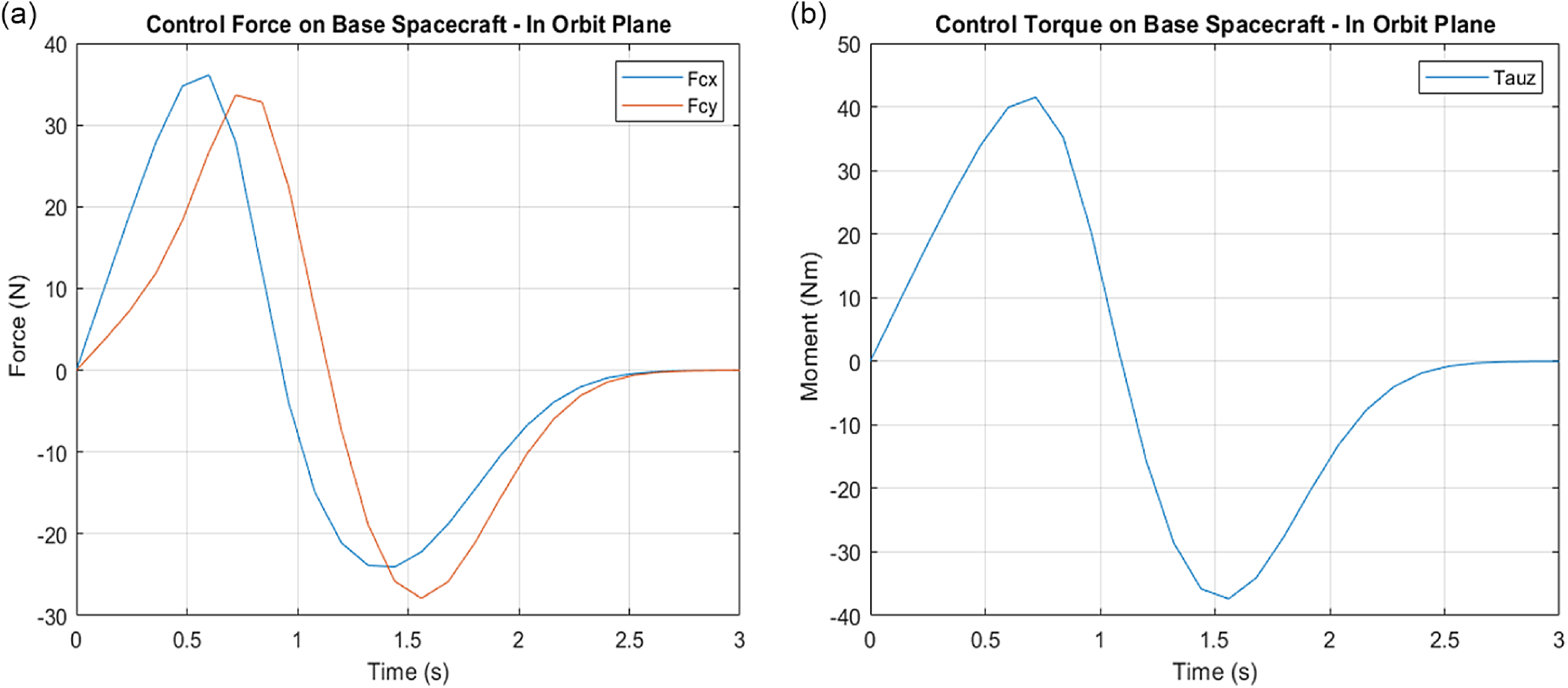
Figure 10. (a–b) Variation of chaser spacecraft control force and moments.
The joint accelerations for each robot are also calculated using Eq. (14) using both OCA and NMPC and are plotted with time in Fig. 11(a–b).
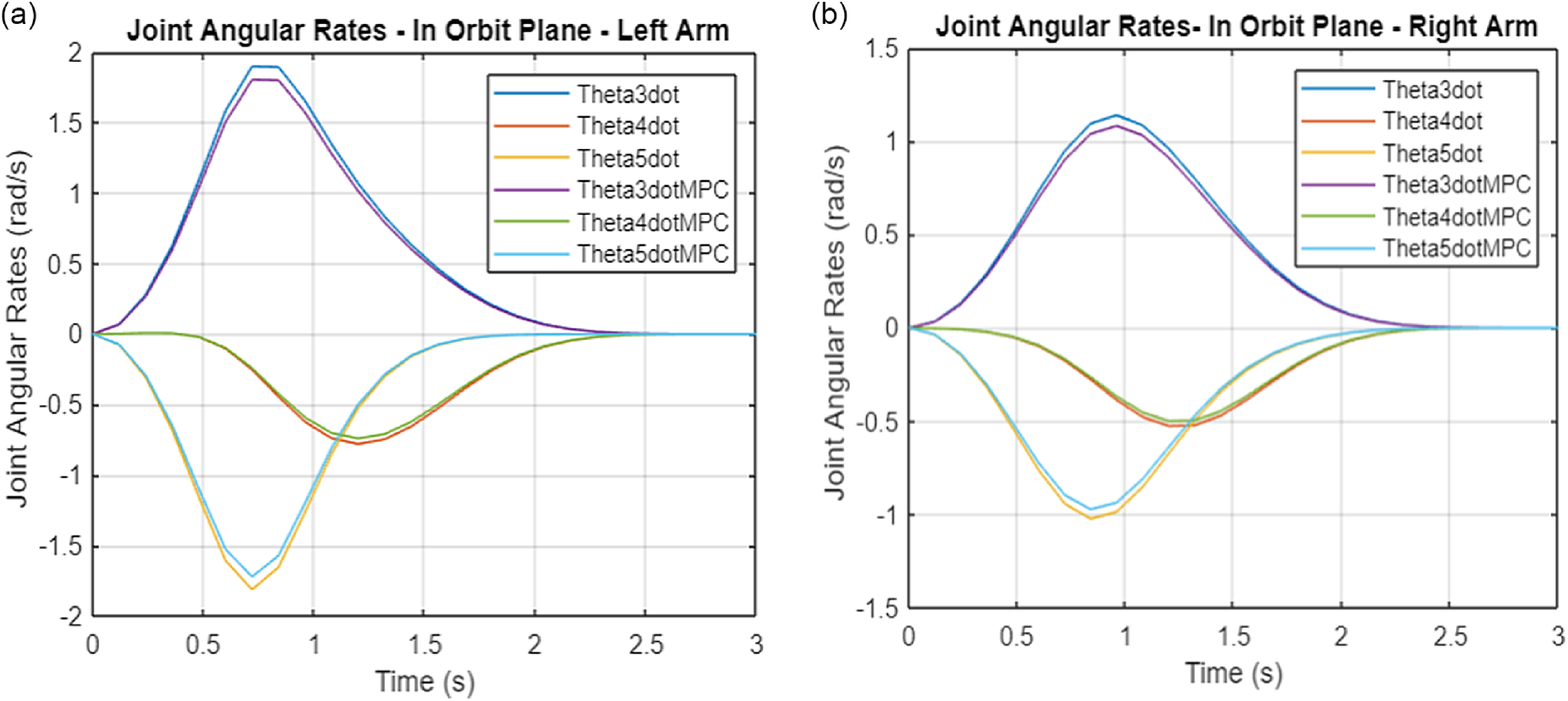
Figure 11. (a–b) Variation of in-orbit joint angular accelerations for left and right arms.
The joint angular rates and angles were obtained by integrating the joint accelerations using Eq. (13) and were plotted in Fig. 12(a–d).
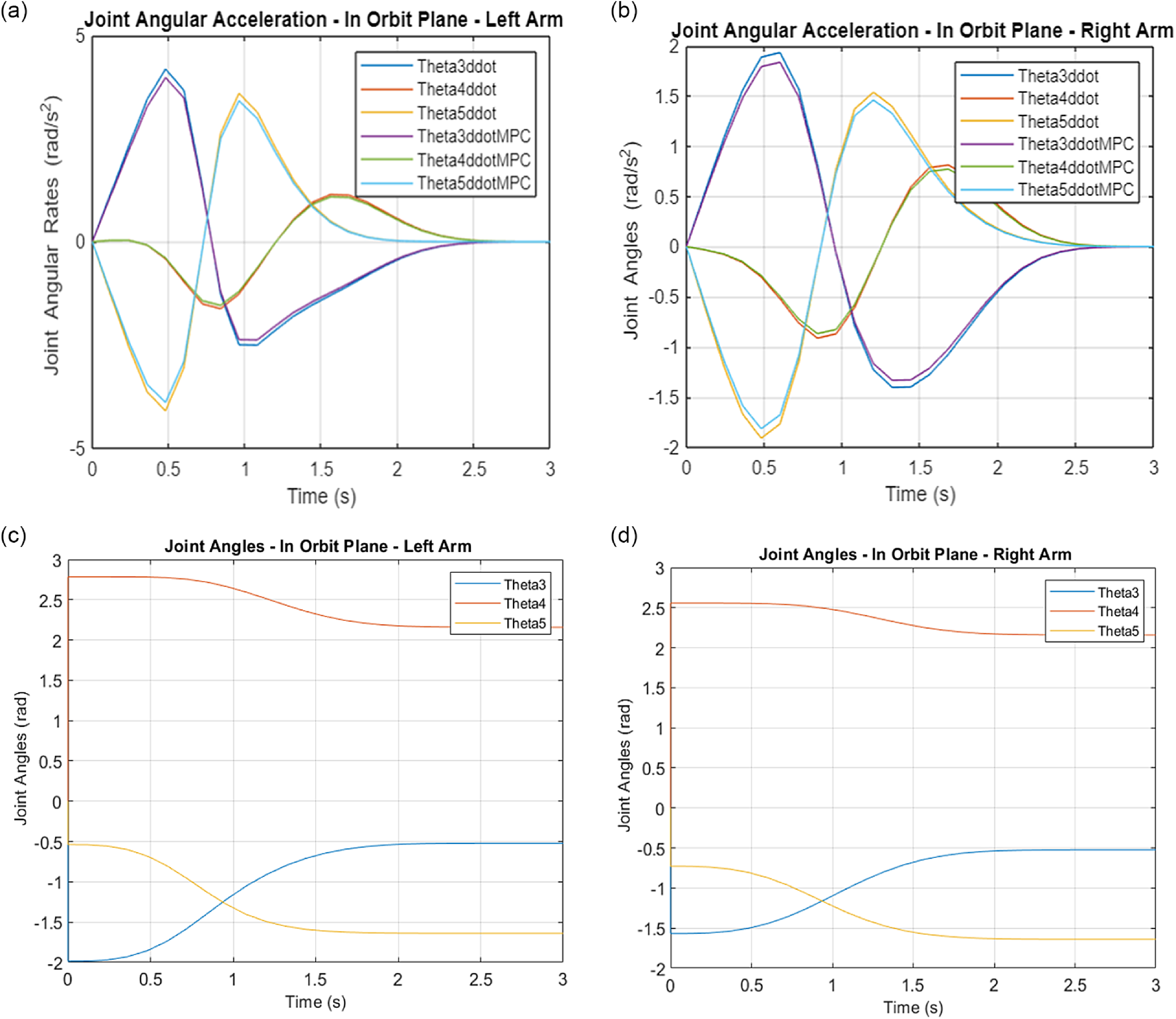
Figure 12. (a–d) Variation of in-orbit joint angular rates and angles for the left and right arms.
3.3 Simulation demonstration of performance of the NMPC in tracking control
In this section, two sets of trajectories provided in [Reference Izadbakhsh and Khorashadizadeh55] are simulated to demonstrate the performance of the developed NMPC in tracking control.
Trajectory 1: The first trajectory is a circle with a radius of 0.2 m centered at (0.8 m 1 m). The simulation results demonstrating tracking performance are presented in Fig. 13(a–e). The simulation results showed that the NMPC algorithm worked very efficiently to follow the circular trajectory. The Cartesian position of the end-effector is plotted in Fig. 13a while the Cartesian end-effector velocities are presented in Fig. 13b. The time variation of joint angles, angular rates, and the minimum norm joint torques values are presented in Fig. 13(c–e).
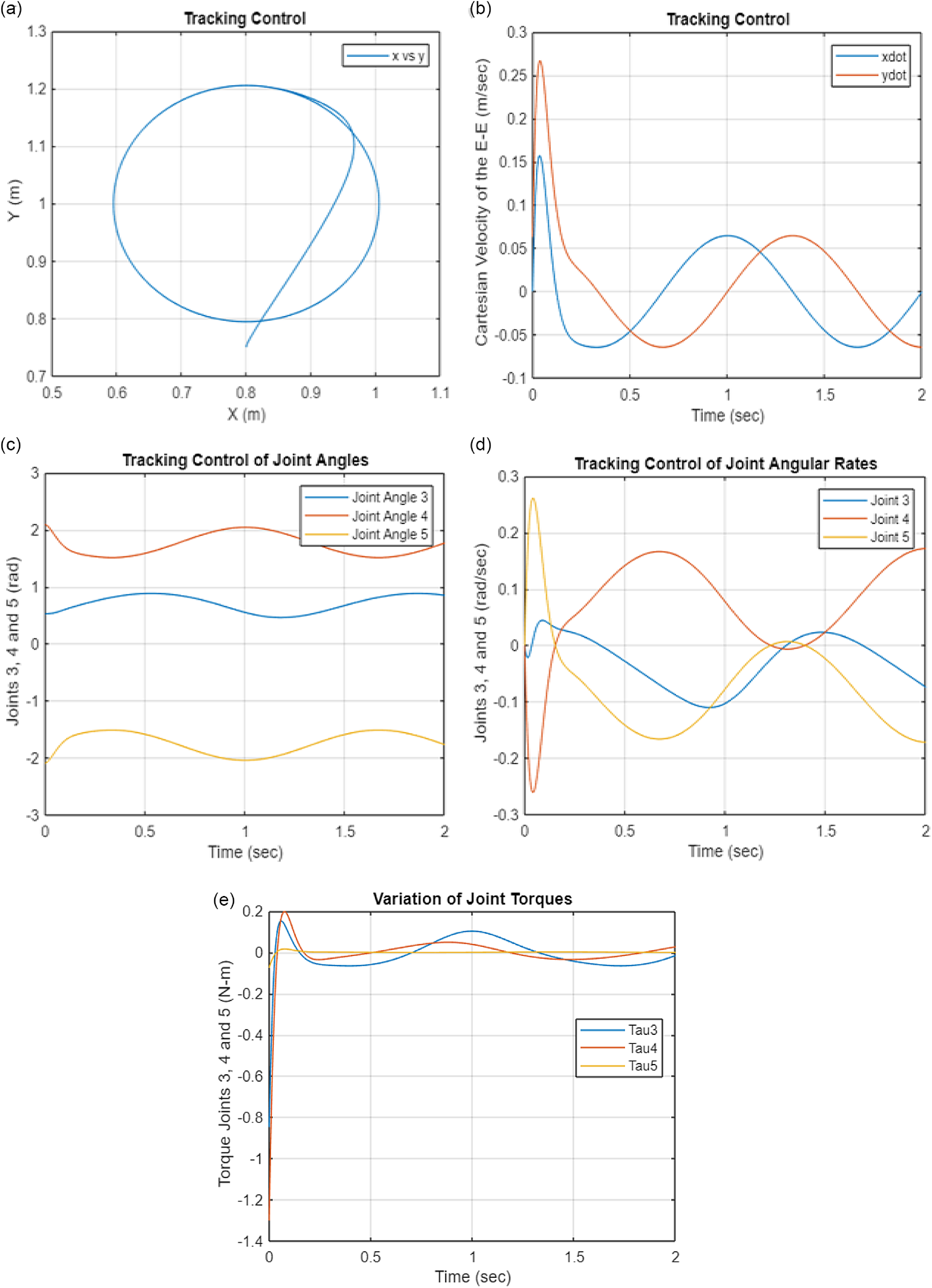
Figure 13. (a–b) Tracking performance. (c–d) Tracking performance – variation of joint angles and rates. (e) Tracking performance – variation of minimum joint torques.
Trajectory 2: The second trajectory is highly intricate and first appeared in [Reference Izadbakhsh and Rafiei56]. This highly complex and intricate trajectory showcases the capability of the proposed NMPC algorithm in tasks requiring accurate tracking of fast and complex trajectories while the robot actuators are subject to torque saturation limits, that is, constraints.
The end-effector is required to track the following trajectory:
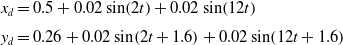 \begin{align} x_{d}&=0.5+0.02\sin\! \left(2t\right)+0.02\sin\! \left(12t\right)\nonumber \\[3pt] y_{d}&=0.26+0.02\sin\! \left(2t+1.6\right)+0.02\sin\! \left(12t+1.6\right) \end{align}
Part 1: The complex trajectory tracking simulation in Part 1 established torque saturation limits $\widetilde{ \boldsymbol{S}}_{\boldsymbol{\max }/\boldsymbol{\min }}$
of ±5 N-m and ±4 N-m for joints 3 and 4, respectively. Figure 14(a–g) displays the simulation results, which show that the NMPC algorithm is highly effective in tracking the complex trajectory. Figure 14(a) displays the Cartesian position of the end-effector, while Fig. 14(b–c) shows the tracking error in Cartesian displacement of the end-effector. Figure 14(d) illustrates time variation of the Cartesian velocity of the end-effector. Figure 14(e–g) displays the changes in joint angles over time, angular rates, and minimum norm joint torque values, respectively.
$\widetilde{ \boldsymbol{S}}_{\boldsymbol{\max }/\boldsymbol{\min }}$
of ±5 N-m and ±4 N-m for joints 3 and 4, respectively. Figure 14(a–g) displays the simulation results, which show that the NMPC algorithm is highly effective in tracking the complex trajectory. Figure 14(a) displays the Cartesian position of the end-effector, while Fig. 14(b–c) shows the tracking error in Cartesian displacement of the end-effector. Figure 14(d) illustrates time variation of the Cartesian velocity of the end-effector. Figure 14(e–g) displays the changes in joint angles over time, angular rates, and minimum norm joint torque values, respectively.
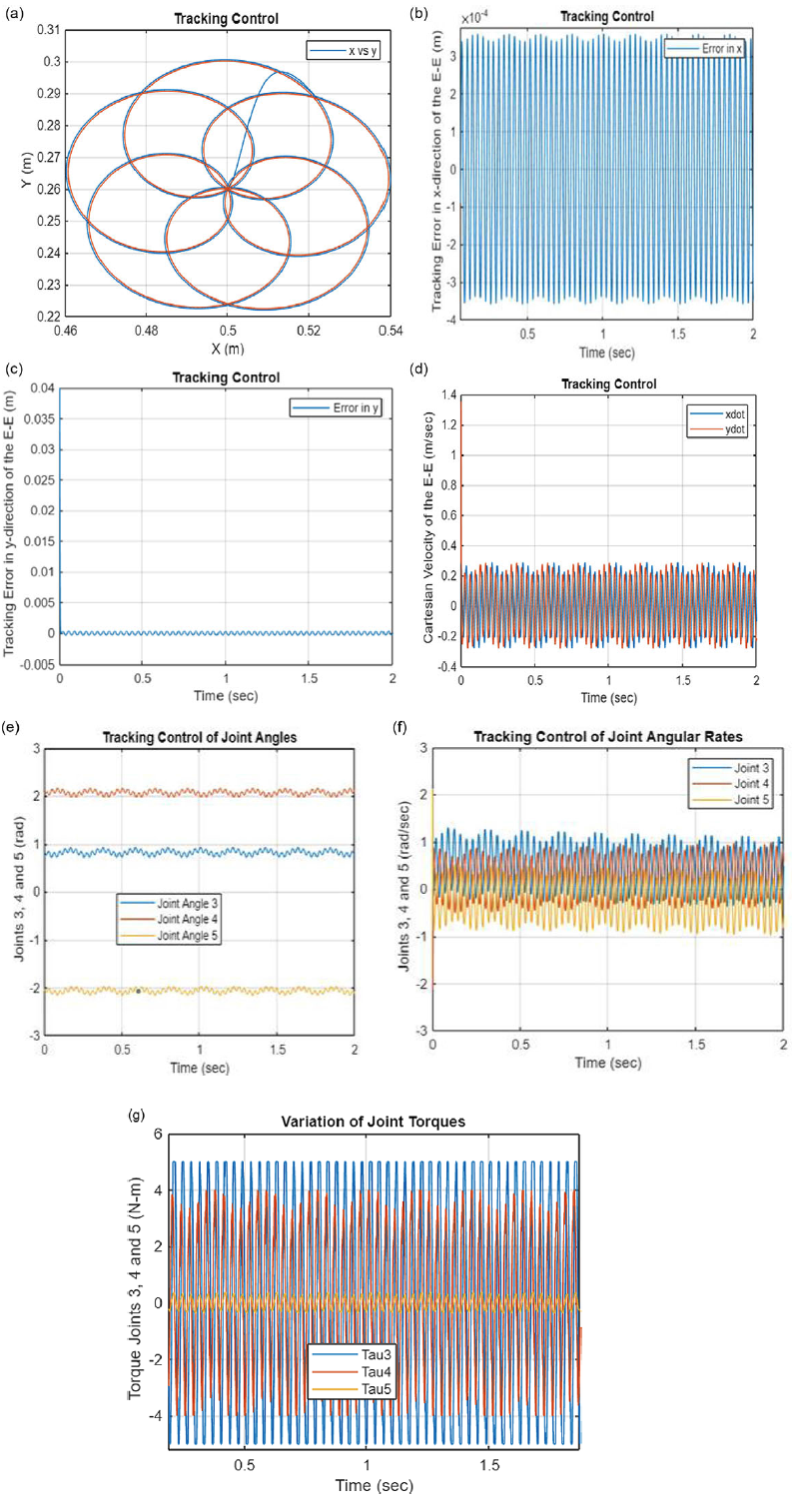
Figure 14. (a–d) Tracking performance. (e–f) Tracking performance – variation of joint angles and rates. (g) Tracking performance – variation of minimum joint torques.
In Part 1, the complex trajectory tracking simulation established torque saturation limits of ±5 N-m and ±4 N-m for joints 3 and 4, as shown in Fig. 14(g), and these limits were not exceeded.
Part 2: To evaluate the impact of these constraints on tracking performance, the joint torque limits for joints 3 and 4 were deliberately reduced to ±3 N-m and ±2 N-m, respectively. Figure 15(a–d) shows the performance of the NMPC controller in tracking the complex trajectory with these tighter joint torque constraints.
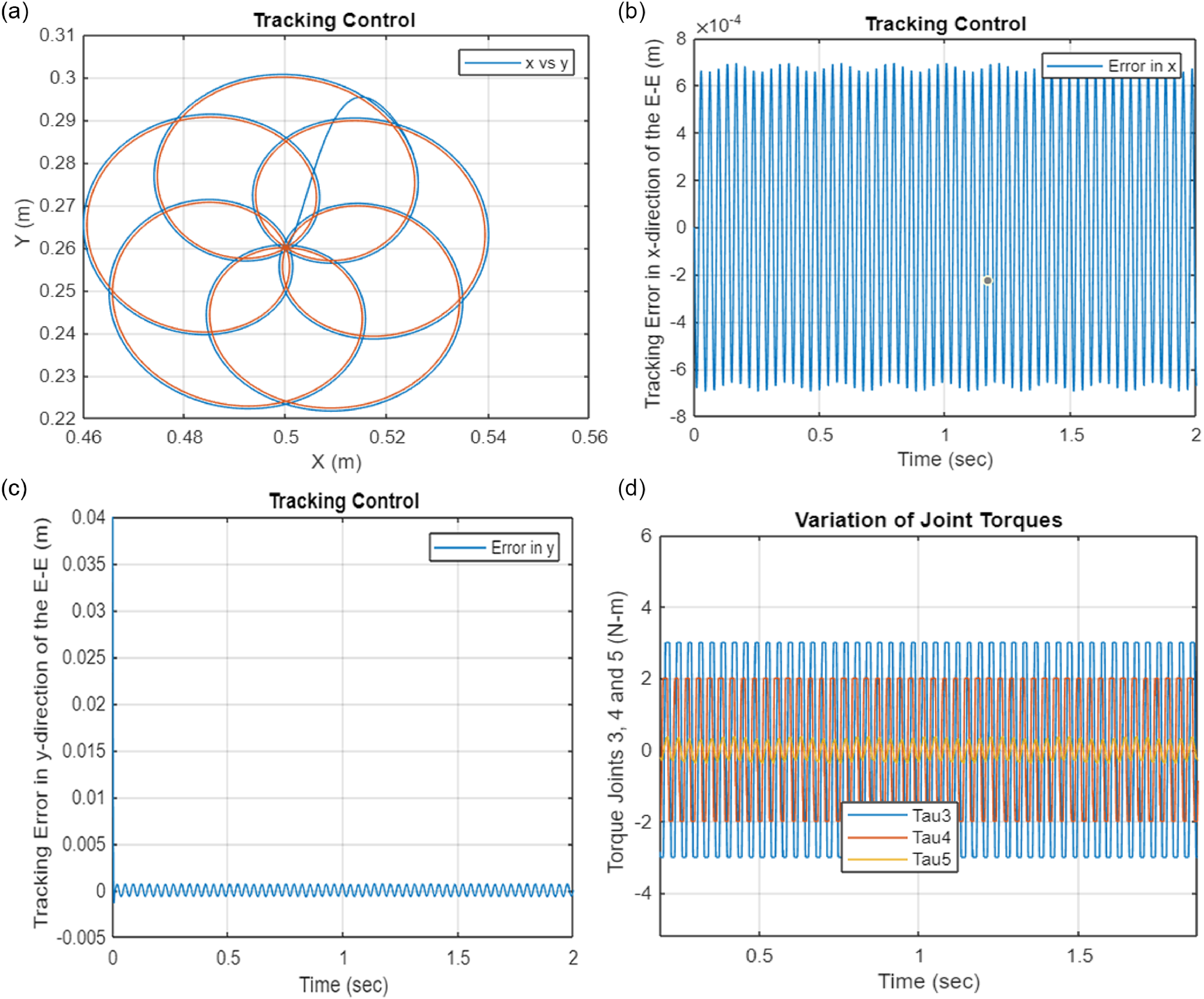
Figure 15. (a) Tracking performance. (b–d) Tracking performance – variation of minimum joint torques.
As seen in Fig. 15(a–d), the tracking performance was negatively affected by the constraint on joint torque saturation limits.
Figure 16(a–b) displays the tracking errors linked to two distinct sets of joint torque constraints. The simulation outcomes demonstrate that implementing the lower torque limits (±2 N-m) rather than the higher limits (±3 N-m) resulted in relatively greater tracking errors. Nevertheless, the overall performance of the NMPC algorithm during a complex trajectory with these strict joint saturation limits remains impressive.
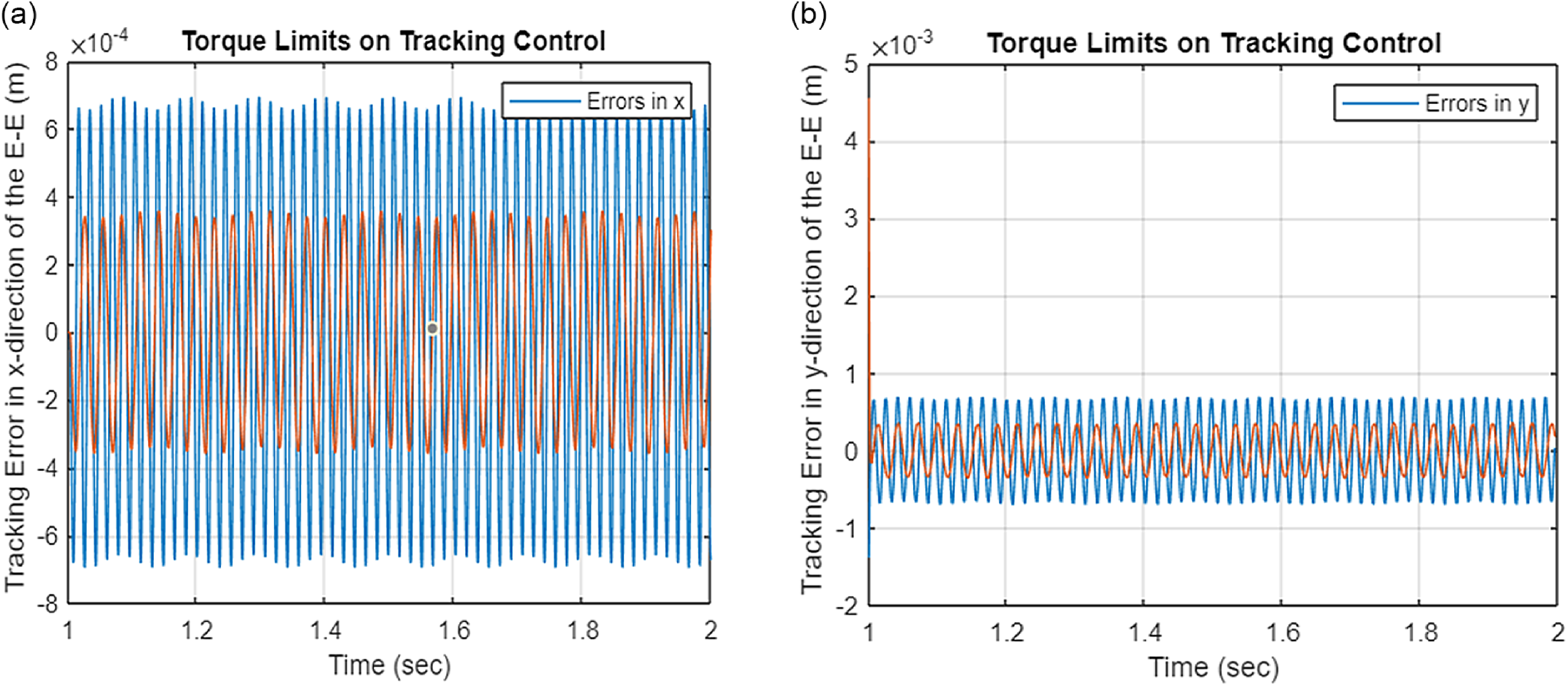
Figure 16. (a–b) Comparisons of tracking performance with different torque constraints.
4. Conclusion and future work
The problem of saturation of spacecraft and robot actuator torques is a formidable challenge during the post-capture stage while controlling a target spacecraft with its uncontrolled large angular and linear momentums.
This paper presented a novel solution to this problem by virtue of two control algorithms based on (i) Optimal Control Allocation (OCA) and (ii) Non-linear Model Predictive Control (NMPC). The main objective of this paper was to develop a robust and computationally efficient real-time control algorithm which minimized a performance index involving the norm of the joint torques, the chaser spacecraft control moments and forces, as well as the contact forces and moments exerted on the payload by two robot manipulators while tracking a desired end-effector pose. The computer simulation results showed that both the OCA and the NMPC algorithms worked efficiently, and the minimum joint torques, spacecraft control moments, and forces and the contact forces and moments were obtained in real-time successfully while the end-effectors were carrying a common payload and successfully tracking a desired payload trajectory. The comparison of the joint torques clearly demonstrated that the minimization scheme by the NMPC algorithm provided the best results (i.e., the lowest joint torques, followed by the OCA and then the conventional least-square technique which is commonly used in the literature).
The NMPC approach did better in minimizing the joint torques although following a slightly different trajectory, yet arriving the same desired destination pose. One can conclude that one of the reasons for this was that the performance index (i.e., the cost function) defined in Eq. (38) involved the future state estimates as well as the control inputs, and the minimization process involved not only the current state errors and current joint torques but also the future state values and joint torques over a specified prediction horizon / future timeline. Thus, the proposed OCA solution can be deemed as a subset solution if the prediction horizon is only assigned to the current time. Furthermore, the NMPC can be regarded as a natural progression from the OCA and be employed depending on the availability of the on-board space computing resources.
It is also observed that the computational complexity of the NMPC was higher than that of the OCA, especially if one wants to employ a continuous non-linear model for the NMPC estimates. One can state that this was perhaps one of the main reasons as to why the literature to date mostly focused on the linear models. However, the dual arm coordination is highly non-linear. The proposed NMPC discretized technique offered exact realizations (of a non-linear model) with elegance and simplicity and yet took into account the full non-linear model of the dual arm coordinating system as demonstrated in the simulations.
The NMPC algorithm was also tested in tracking a highly complex and intricate trajectory while the robot actuators were under strict torque saturation limits. The computer simulation revealed that while the joint torque saturation limits negatively impacted the tracking performance, the overall performance of the NMPC algorithm during the complex trajectory remained impressive despite these strict constraints.
The developed NMPC is facing certain limitations, which we plan to address in our upcoming research work. The performance of NMPC can be negatively impacted if there are inaccuracies in the modeling process. Furthermore, NMPC necessitates offline tuning of its parameters and may not handle disturbances effectively if they are not precisely modeled. Additionally, the current saturation policy lacks a systematic approach for handling output constraints and does not take into account future predictions of inputs.
Acknowledgments
This research was supported by the National Science and Engineering Research Council of Canada.
Authors’ contributions
All authors contributed to the study conception and design. Initial material preparation and analysis were performed by Serdar Kalaycioglu. The first draft of the manuscript was written by Serdar Kalaycioglu and Anton de Ruiter. All authors commented on previous versions of the manuscript. All authors read and approved the final manuscript.
Conflicts of interest
The authors declare no conflict of interest.
Ethical considerations
None.
Appendix
Table I. System parameters.
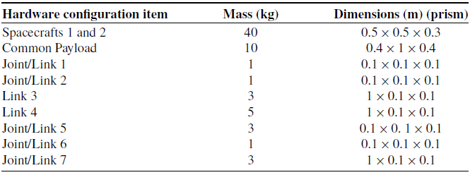


 Open access