


1. Introduction
The ability to autonomous navigation, in which the robot can learn and accumulate knowledge in real environments for selecting optimal behavior autonomously, is a prerequisite for mobile robots to perform tasks smoothly in all applications [Reference Kanmani, Malathi, Rajkumar, Thamaraiselvan and Rahul1]. Currently, several excellent methods have been proposed for autonomous navigation, such as fuzzy logic [Reference Srine and Alimi2], genetic algorithms [Reference Wang, Soh, Wang and Wang3, Reference Wang, Luo, Li and Cai4], random trees [Reference Pandey, Sonkar, Pandey and Parhi5], and neural networks [Reference Tom and Branko6–Reference Luo and Yang8]. However, these methods usually need to assume complete environmental configuration information, which has to be adapted by agents in a large number of practical applications. Therefore, how to improve the self-learning ability and adaptability of robot navigation in an unknown environment has become a key technology for scholars to study. In particular, the self-learning ability and self-adaptability of robots are determined by the intelligence level of a robot’s perception and response to the environment determines. Cognition and learning ability are the main ways in which humans and animals acquire knowledge, and it is also a significant sign of their intelligence. Therefore, many scholars have begun to simulate biological cognition and behavioral learning models in order to conduct extensive research on mobile robot navigation systems [Reference Shao, Yang and Shi9–Reference Chen and Abdelkader12].
Reinforcement learning algorithm is the optimal strategy to approach the target by interactive learning by maximizing the cumulative reward of agents in the environment. The algorithm is a model of “closed-loop learning” paradigm. Reinforcement learning is applied to the learning ability of robots in unknown environments. At present, reinforcement learning has been widely used in robot autonomous navigation and has achieved many important results. Xu et al. [Reference Xu13]. proposed a reactive navigation method for mobile robots based on reinforcement learning and successfully applied it to the CIT-AVT-VI mobile robot platform; Wen et al. [Reference Wen, Chen, Ma, Lam and Hua14] designed Q-learning obstacle avoidance algorithm based on KEF-SLAM for NAO robot autonomous walking in unknown environment; Cherroun et al. [Reference Cherroun and Boumehraz15] studied autonomous navigation based on fuzzy logic and reinforcement learning. Although the reinforcement learning-based navigation method can successfully navigate autonomously, the reinforcement learning Q-learning learning information is stored in the Q table and needs to be updated continuously.
In 1938, Skinner first proposed the concept of operational conditional reflection (OCR) and thus created the theory of OCR. Referring to Pavlov’ s concept of “reinforcement,” he divided “reinforcement” into positive reinforcement and negative reinforcement. Positive reinforcement increased the response probability of organisms to stimuli, and negative reinforcement increased the response of organisms to eliminate the stimuli. Stimulus produces response, which affects the probability of stimulus, which is the core of Skinner’s operational conditioned reflex theory [Reference Skinner16]. Since the mid-1990s, Heisenberg et al. have been focusing on the computational theory and model of Skinner’s OCR [Reference Heisenberg, Wolf and Brembs17]. Moreover, Touretzky et al. have further developed the computational model of Skinner’s OCR theory [Reference Touretzky, Daw and Tira-Thompson18]. Later, many scholars have carried out extensive research on the computational model of operational conditioned reflexes [Reference Zhang, Ruan, Xiao and Huang19–Reference Cai, Ruan, Yu, Chai and Zhu32]. Robots are showing more self-learning ability and self-adaptability, similar to organisms. Zhang et al. proposed the Cyr-an outstanding representative, which enables biological agents to learn from the results of previous actions by means of operational conditioned reflexes [Reference Zhang, Ruan, Xiao and Huang19]. Ruan et al. Have carried out a series of studies on the operational conditioned reflex model [Reference Ruan, Dai and Yu24–Reference Cai, Ruan, Yu, Chai and Zhu32], including the design and calculation model based on the operational conditioned reflex mechanism, combined with probabilistic automata, neural network, and extended Kalman filter. In 2013, Ruan et al. designed a bionic learning model based on operating conditioned reflex learning automata. When applied to self-balancing control and autonomous navigation of two-wheeled robots, the results show that robots can learn autonomously like animals, and their adaptability is better than reinforcement learning. In 2016, Ruan et al. designed Skinner-Ransac algorithm based on Skinner’s operating conditioned reflex principle and extended Kalman filter, which can simultaneously realize positioning and map creation (SLATM), and the pose estimation results of slam can meet the needs of mobile robot autonomous navigation. In 2018, Cai Jianxian et al. designed a cognitive development model for autonomous navigation based on biological cognition and development mechanism. This model can enable robots to simulate animals to automatically acquire knowledge and accumulate experience from unknown environments and acquire the skills of autonomous navigation through cognitive development.
Based on the idea of operational conditioned reflex cognitive model and hierarchy proposed by Ruan et al. [Reference Ruan, Dai and Yu24–Reference Cai, Ruan, Yu, Chai and Zhu32], this paper constructs a cognitive model based on operational conditioned reflex and hierarchy to solve the self-learning and adaptive problems of mobile robot autonomous navigation system in unknown complex environment. An operational conditioned reflex cognitive model uses the idea of dividing and conquering; it divides the navigation tasks of mobile robots in complex environments into sub-tasks at different levels and solves each sub-task in a small state subspace in order to reduce the dimension of the state space. A cognitive learning algorithm is designed to simulate the thermodynamic process and achieve the optimal navigation strategy for an online search. Based on the formation of cognitive processes, we investigated autonomous path planning processes of mobile robots. The results show that the hierarchical structure can reduce the learning difficulty and accelerate the learning speed of mobile robots in unknown and complex environments. At the same time, robots can automatically acquire knowledge and accumulate knowledge from the environment, like animals. Experience gradually forms, develops, and perfects the robot’s autonomous path planning skills.
2. Basic principles of hierarchical reinforcement learning
Path planning of mobile robots involves finding an optimal path, which enables the robot to reach the target point without collision and optimize performance indicators, such as distance, time, and energy consumption. Distance is the most commonly used criteria. In order to better accomplish this task, in the process of reinforcement learning, robots need to perform different actions in order to obtain more information and experience and to promote higher future returns. On the other hand, they need to accumulate and execute the current actions with the highest returns according to their own experience. This is called the tradeoff between exploration and exploitation [Reference Rasmussen, Voelker and Eliasmith33]. Too little exploration hinders the convergence of the system in regard to the optimal strategy and too much exploration leads to a higher dimension of the general state space. The size of the state space affects the convergence rate of the bionic learning system. When the state space is too large, mobile robots can spend a lot of time exploring; the learning efficiency is consequently low and it is difficult to converge. In order to solve this problem, a hierarchical reinforcement learning structure is proposed [Reference Li, Narayan and Leong34]. The aim is to reduce the learning difficulty of the reinforcement learning systems in a complex environment through hierarchical learning. The core idea of the hierarchical reinforcement learning method is to use an abstract method to divide the whole task into different levels of sub-tasks and solve each sub-task in a small state subspace, in order to obtain reusable sub-task strategies and speed up the solution to the problem.
State space decomposition, temporal abstraction, and state abstraction are commonly used techniques in hierarchical reinforcement when a robot is learning to achieve hierarchy. The state space decomposition method divides the state space into several different subspaces and solves the task in the subspace of lower dimensions. The temporal abstraction principle involves grouping the action space set in order to realize the execution of multi-step actions in the process of agent reinforcement learning, thus reducing the consumption of computing resources. The state abstraction method ignores the state space variables that are not related to a sub-task, which reduces the dimensionality of the state space. Although the above three methods layer the system with different methods, they also realize the function of reducing the complexity of the system state space and accelerating the learning speed of the system.
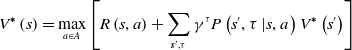
Sequential decision-making problems are usually modeled by Markov Decision Processes (MDP) [Reference Sagnik and Prasenjit35]. When the execution of action strategies extends from a point in time to continuous time, an MDP model also extends to a Semi-Markov Decision Processes (SMDP) model. An SMDP model can solve the problem of learning, which needs to complete action execution in multiple time steps and make up for the deficiency of reinforcement learning, which only assumes that an action is completed in a single time step in the framework of the MDP model. The Bellman optimal equation of value function, based on the SMDP model, is shown in Eq. (1), the Bellman optimal equation of state-action pair function is shown in Eq. (2), and the Q-learning iteration equation is shown in Eq. (3):
 \begin{equation} V^{\boldsymbol{*}}\left(s\right)=\max _{a\in A}\left[R\left(s,a\right)+\sum _{{\boldsymbol{{s}}}^{\prime},\tau }\gamma ^{\tau }P\left(s^{\prime},\tau \left| s,a\right.\right)V^{\boldsymbol{*}}\left(s^{\prime}\right)\right] \end{equation}
 \begin{equation} Q^{\boldsymbol{*}}\left(s,a\right)=R\left(s,a\right)+\sum _{{\boldsymbol{{s}}}^{\prime},\tau }\gamma ^{\tau }P\left(s^{\prime},\tau \left| s,a\right.\right)\max _{a\in A}Q^{\boldsymbol{*}}\left(s^{\prime},a'\right) \end{equation}
 \begin{equation} Q_{k+1}\left(s,a\right)=\left(1-\alpha \right)Q_{k}\left(s,a\right)+\alpha \left[r_{t}+\gamma r_{t+1}+\cdots +\gamma ^{\tau -1}r_{t+\tau -1}+\gamma ^{\tau }\max _{a\in A}Q^{\boldsymbol{*}}\left(s^{\prime},a'\right)\right] \end{equation}
In the formula, $\tau$
is the random waiting time, indicating the time interval after the agent executes action a in state s;
$\tau$
is the random waiting time, indicating the time interval after the agent executes action a in state s; $P(s^{\prime},\tau | s,a)$
is the transition probability from action a in state s to action a after the agent waits for time
$P(s^{\prime},\tau | s,a)$
is the transition probability from action a in state s to action a after the agent waits for time $\tau$
; and
$\tau$
; and $R(s,a) = E[r_{t}+\gamma r_{t+1}+\cdots +\gamma ^{\tau }r_{t+\tau }]$
is the corresponding reward value.
$R(s,a) = E[r_{t}+\gamma r_{t+1}+\cdots +\gamma ^{\tau }r_{t+\tau }]$
is the corresponding reward value.
HRL problems are often modeled based on the SDMP model. HRL (Hierarchical Reinforcement Learning) adopts the strategy of divide and conquer; it divides the planning tasks of agents into sub-tasks at different levels and solves each sub-task in a smaller state subspace, thus realizing the function of reducing the dimension of the state space.
3. Hierarchical structure cognitive model design
3.1. Structure of the cognitive model
The complexity of the working environment, the size of the state space, and the size of the behavior space of a mobile robot affect the robot’s learning rate. When the state space is too large, mobile robots will spend a lot of time exploring, resulting in the “dimension disaster” problem; when the behavior space is too large, mobile robots need to try to learn many times, which makes cognitive model learning inefficient and difficult to converge to the optimal strategy. So robots need to acquire the ability to learn in complex and unknown environments.
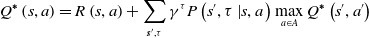
In view of these practical problems, considering that the path planning task of mobile robots is carried out in an unknown environment with static or dynamic obstacles, the obstacle avoidance problem for static and dynamic obstacles should be considered in the design of the hierarchical cognitive model. In this paper, the path planning tasks of mobile robots are divided into three basic sub-tasks: “static obstacle avoidance” for static obstacles, “dynamic obstacle avoidance” for dynamic obstacles, and “targeting point” motion. Decomposed into small-scale state subspaces, each sub-task is solved in each state subspace independently. Furthermore, considering that the bionic strategy is a trial-and-error learning process, the mobile robot performs complex behaviors. Therefore, the complex behavior strategy is decomposed into a series of simple behavior strategies and independent learning training. The structure of the hierarchical structure cognitive model of the design is shown in Fig. 1.
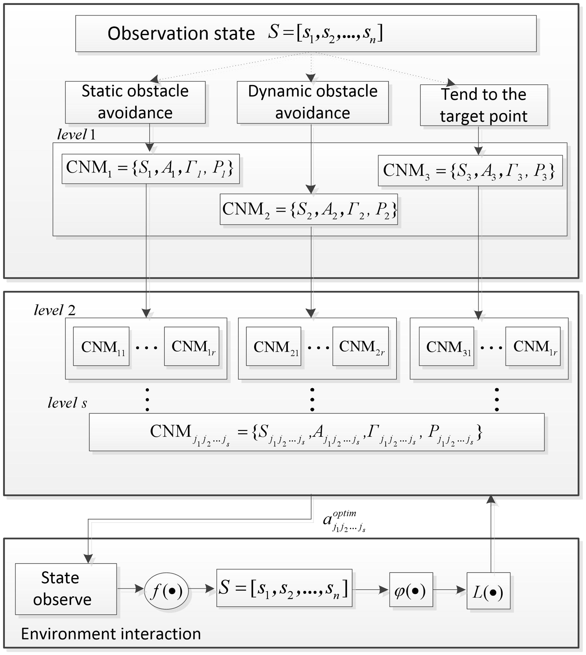
Figure 1. Hierarchical cognitive model.
In Fig. 1, the HCNM learning model includes two functional layers: sub-task selection and behavior decomposition. The sub-task selection layer includes three sub-task selection modules, “static obstacle avoidance,” “dynamic obstacle avoidance,” and “trend target point.” According to the observed environmental state decision output, the corresponding sub-task is selected and the mobile robot is then selected according to the sub-task. The planning strategy selects the behavior and executes it; the behavior set of the sub-task selection layer adopts a roughly divided form. According to the selection result of the sub-task’s behavior, the behavior decomposition layer is further finely divided and the number of layers of the refined score is determined according to the degree of complexity of the actual behavior.
Therefore, the HCNM learning model is actually composed of multiple single cognitive systems. If the hierarchical cognitive model is regarded as consisting of seven parts, HCNM = <A, S, Γ, P, f, $\phi$
, L>, all CNM learning systems share elements {f,
$\phi$
, L>, all CNM learning systems share elements {f, $\phi$
, L}, and other elements {S, A, Γ, P} are applied to the corresponding CNM learning system, respectively. Assuming that the number of optional behaviors in the behavior set is r, there are three CNM learning systems:
$\phi$
, L}, and other elements {S, A, Γ, P} are applied to the corresponding CNM learning system, respectively. Assuming that the number of optional behaviors in the behavior set is r, there are three CNM learning systems: $\{\mathrm{CNM}_{1}\mathrm{,CNM}_{2}\mathrm{,CNM}_{3}\}$
for Level 1 (sub-task selection layer) of the HCNM learning model; Level 2 is the first level of the behavior decomposition layer of the HCNM learning model, and there are 3r CNM learning systems:
$\{\mathrm{CNM}_{1}\mathrm{,CNM}_{2}\mathrm{,CNM}_{3}\}$
for Level 1 (sub-task selection layer) of the HCNM learning model; Level 2 is the first level of the behavior decomposition layer of the HCNM learning model, and there are 3r CNM learning systems: $\{\mathrm{CNM}_{11}\mathrm{,}\ldots \mathrm{,CNM}_{1r}, \mathrm{CNM}_{21}\mathrm{,}\ldots \mathrm{,CNM}_{2r}, \mathrm{CNM}_{31}\mathrm{,}\ldots \mathrm{,CNM}_{3r}\}$
. By analogy, there are 3rs CNM learning systems for the Level s layer. Through the s layer, the corresponding behavior a is selected and used as the environment, and new state information s is observed. Based on this, the orientation evaluation
$\{\mathrm{CNM}_{11}\mathrm{,}\ldots \mathrm{,CNM}_{1r}, \mathrm{CNM}_{21}\mathrm{,}\ldots \mathrm{,CNM}_{2r}, \mathrm{CNM}_{31}\mathrm{,}\ldots \mathrm{,CNM}_{3r}\}$
. By analogy, there are 3rs CNM learning systems for the Level s layer. Through the s layer, the corresponding behavior a is selected and used as the environment, and new state information s is observed. Based on this, the orientation evaluation $\varphi$
of the environment is obtained, and the updating
$\varphi$
of the environment is obtained, and the updating $L$
of learning knowledge is completed. In this way, after many rounds of interactive learning with the environment, our model can make the most optimal decision.
$L$
of learning knowledge is completed. In this way, after many rounds of interactive learning with the environment, our model can make the most optimal decision.
(1) The symbols in the HCNM learning model are defined as follows:
-
i. f: The state transition function of the HCNM learning model, $f\colon S(t)\times A(t)| P\rightarrow S(t+1)$
. It shows that the state
$s(t+1)\in S$
of t + 1 time is determined by the state
$s(t)\in S$
at time t and the probabilistic operation
$\alpha (t)| P\in A$
at time t, which is independent of the state and operation before t time.
$f\colon S(t)\times A(t)| P\rightarrow S(t+1)$
. It shows that the state
$s(t+1)\in S$
of t + 1 time is determined by the state
$s(t)\in S$
at time t and the probabilistic operation
$\alpha (t)| P\in A$
at time t, which is independent of the state and operation before t time. -
ii.
$\phi$
: The HCNM learning model orientation mechanism,
$\phi =\{\phi _{1},\phi _{2}\ldots,\phi _{\mathrm{n}}\}, \phi _{i}\in \phi$
, represents the orientation value of the state
$s_{i}\in S$
, which represents the tendency of the state to update the probability vector Pi, satisfying:
$0\lt \phi _{i}\lt 1$
. -
iii. L: The operation conditioned reflex learning mechanism of the HCNM learning model,
$L\colon (t)\rightarrow (t+1)$
. Update and adjust the probability according to
$P(t+1)=L[P(t),\phi (t),a(t)]$
.


(2) The elements of the HS-CNM learning models belonging to different CNM learning systems are as follows:
Level 1:  $S_{1}$, $S_{2}$, and $S_{3}$ represent the internal discrete state set of three sub-tasks, respectively: $S_{{i}'}=\{s_{i'{i}}| \,i'=1,2,3, i=1,2,\cdots ,n\}, S_{{i}'}$ is a non-empty set composed of all possible discrete states of the control system, and $s_{i'{i}} \in S_{{i}'}$indicates that the HCNM system is in the first state at a certain time. $A_{{i}'}$ represents the behavior set of Level 1 hierarchy tasks: $A_{{i}'}=\{\alpha _{{i}'{j_{1}}}| j_{1}=1,2,\cdots ,r\}, \alpha _{{i}'{j_{1}}}$ is the j 1 operation of sub-task ${i}'$. $\mathit{\Gamma }_{{i}'}$ represents a set of conditional state-action random mappings for Level 1 sub-tasks. It means that $\mathrm{CNM}_{{i}'}$ implements operation $\alpha _{{i}'{j_{1}}}\in A_{{i}'}$ according to probability $P_{{i}'}$ under the condition that the state is $s_{i'{i}} \in S_{{i}'}$. $P_{{i}'}$ denotes the probability vector of the operation behavior set $A_{{i}'}, {p}_{{i}'{j_{1}}}\in P_{{i}'}(j_{1}=1,{\ldots},r)$ and denotes the probability value of the implementation of operation behavior $\alpha _{{j_{1}}}$, satisfying: $0\lt p_{{j_{1}}}\lt 1, \sum _{j1=1}^{r}p_{{j_{1}}}=1$.
Level 2:  $\mathrm{CNM}_{{i}'{j_{1}}}=\{S_{{i}'{j_{1}}},\,A_{{i}'{j_{1}}},\,\mathit{\Gamma }_{{i}'{j_{1}}},\,P_{{i}'{j_{1}}}\}$: The output behavior of Level 1 is $\alpha _{{i}'{j_{1}}}$ as the internal state set of the $\mathrm{CNM}_{{i}'{j_{1}}}$ learning system in the Level 2 layer: $S_{{i}'{j_{1}}}=\{a_{{i}'{j_{1}}}\}$. $A_{{i}'{j_{1}}}$ represents the set of operation behavior of the Level2 level CNM learning system: $A_{{i}'{j_{1}}}=\{\alpha _{{i}'{j_{1}}{j_{2}}}| j_{2}=1\mathrm{,}2\mathrm{,}\cdots \mathrm{,}r\}$. $\mathit{\Gamma }_{{i}'{j_{1}}}$ represents the conditional state of the Level2 level CNM learning system – the random mapping set of operation behavior: $\mathit{\Gamma }_{{i}'{j_{1}}}\!\colon \{a_{{i}'{j_{1}}}\rightarrow a_{{i}'j_{1}j_{2}}(P_{{i}'{j_{1}}})\mathrm{,}\,j_{2}=(1\mathrm{,}\ldots \mathrm{,}r)\}$. $P_{{i}'{j_{1}}}$ denotes the probability vector of operation behavior set $A_{{i}'{j_{1}}}$ and ${p}_{{i}'{j_{1}}{j_{2}}}\in P_{{i}'{j_{1}}}$ denotes the probability value of operation behavior set $\alpha _{{i}'{j_{1}}{j_{2}}}$, which satisfies: 0< $p_{{i}'{j_{1}}{j_{2}}}$<1, $\sum _{j_{2}=1}^{r}p_{{i}'{j_{1}}{j_{2}}}=1$.
The Levels layer  $\mathrm{CNM}_{{i}'{j_{1}}{j_{2}}\ldots {j_{s-1}}}=\{S_{{i}'{j_{1}}{j_{2}}\ldots {j_{s-1}}},\,A_{{i}'{j_{1}}{j_{2}}\ldots {j_{s-1}}},\,\mathit{\Gamma }_{{i}'{j_{1}}{j_{2}}\ldots {j_{s-1}}},\,P_{{i}'{j_{1}}{j_{2}}\ldots {j_{s-1}}}\}$: The operation behavior of the Level(s-1) layer is $\alpha _{{i}'{j_{1}}{j_{2}}\ldots {j_{s-2}}}$ as the internal state set of the CNM learning system in the Levels layer: $S_{{i}'{j_{1}}{j_{2}}\ldots {j_{s-1}}}=\{a_{{i}'{j_{1}}{j_{2}}\ldots {j_{s-1}}}\}$. $A_{{i}'{j_{1}}{j_{2}}\ldots {j_{s-1}}}$ represents the set of operation behaviors of the Levels level CNM learning system: $A_{{i}'{j_{1}}{j_{2}}\ldots {j_{s-1}}}=\{\alpha _{{j_{1}}{j_{2}}\ldots {j_{s\mathit{-}1}}}| j_{s\mathit{-}1}=1\mathrm{,}2\mathrm{,}\cdots \mathrm{,}r\}$. $\mathit{\Gamma }_{{i}'{j_{1}}{j_{2}}\ldots {j_{s-1}}}$ represents the conditional state of the Levels CNM learning system – the random mapping set of operation behavior $\mathit{\Gamma }_{{i}'{{j}_{1}}{{j}_{2}}\mathit{.}\mathit{.}\mathit{.}{{j}_{{s}\mathit{-}1}}}\!\colon \{a_{{i}'{{j}_{1}}{{j}_{2}}\mathit{.}\mathit{.}\mathit{.}{{j}_{{s}\mathit{-}1}}}\rightarrow a_{{i}'{{j}_{1}}{{j}_{2}}\mathit{.}\mathit{.}\mathit{.}{{j}_{{s}}}}(P_{{i}'{{j}_{1}}{{j}_{2}}\mathit{.}\mathit{.}\mathit{.}{{j}_{{s}\mathit{-}1}}})\mathrm{,}\,j_{s-1}=(1\mathrm{,}\ldots \mathrm{,}r)\}$. $P_{{i}'{j_{1}}{j_{2}}\ldots {j_{s-1}}}$ denotes the probability vector of the operation behavior set $A_{{i}'{j_{1}}{j_{2}}\ldots {j_{s-1}}}$ and ${p}_{{i}'{j_{1}}{j_{2}}\ldots {j_{s\mathit{-}1}}}\in P_{{i}'{j_{1}}{j_{2}}\ldots {j_{s-1}}}$ denotes the probability value of implementing the operation behavior $\alpha _{{i}'{j_{1}}{j_{2}}\ldots {j_{s\mathit{-}1}}}$, which satisfies: 0< $p_{{i}'{j_{1}}{j_{2}}\ldots {j_{s\mathit{-}1}}}$<1, $\sum _{{i}'=1}^{3}\sum _{j_{s-1}=1}^{r}p_{{i}'{j_{1}}{j_{2}}\ldots {j_{s\mathit{-}1}}} = 1$.
The working process of the HCNM learning model can be briefly summarized as follows: t = 0 time; the state condition signal  ${s}_{{i}}$ first activates the CNM learning system of the Level1 layer to determine the sub-tasks to be performed. Then, it moves into the behavior decomposition layer and chooses the refined behavior. The initial probability of behavior selection is the same; that is, $p_{{i}'{j_{1}}}=\dfrac{1}{r}\left(p_{{i}'{j_{1}}}\in P,\,j_{1}=1,\ldots ,r\right)$; $p_{{i}'{j_{1}}{j_{2}}}=\dfrac{1}{r}\left(p_{{i}'{j_{1}}{j_{2}}}\in P_{{i}'{j_{1}}},\,j_{1}=1,\ldots ,r,\,j_{2}=1\mathrm{,}\ldots \mathrm{,}r\right)$. According to the probability vector $P_{{i}'} = (p_{{i}'\mathrm{1}},\,p_{{i}'\mathrm{2}},\ldots ,\,p_{{i}'{r}})$, the learning system randomly selects an operation behavior (assumed to be $a_{{i}'{j_{1}}}$) from the behavior set ${A}_{{i}'}$ and transfers it to the next layer. Behavior $a_{{i}'{j_{1}}}$ acts as the internal state signal of the next layer of the CNM learning system, activates the corresponding $\mathrm{CNM}_{{i}'{j_{1}}}$learning system, and then, the CNM learning system randomly selects a behavior (assumed to be $a_{{i}'{j_{1}}{j_{2}}}$) from the operation behavior set ${A}_{{i}'{{j}_{1}}}$, according to the probability vector $P_{{i}'{j_{1}}}=[p_{{{i}'_{1}}1},\,p_{{i}'2}\mathrm{,}\ldots ,\,p_{{i}'r}]$, and continues to transport it to the next layer. Similar operations range from Level 2 to Level s, and ultimately output behavior $a_{{i}'{j_{1}}{j_{2}}\ldots {j_{{s}\mathit{-}\text{1}}}}$ as a control signal acting on the control system. After several rounds of trial learning, the optimal decision $a_{{i}'j_{1}j_{2}\ldots j_{{s}}}^{\textit{optim}}$ of each sub-task is finally learned.
In order to illustrate the learning process of the HCNM learning model more clearly, the following definition is given:
Definition 1: Behavior path: From Level 1 to Level s, Sequence  $a_{{i}'{j_{1}}},a_{{i}'{j_{1}}{j_{2}}},\ldots ,a_{{i}'{j_{1}}{j_{2}}\ldots {j_{{s}\mathit{-}\text{1}}}}$, which is composed of behaviors selected by the CNM learning system, is defined as a behavior path, expressed in $\phi _{{i}'{j_{1}}{j_{2}}\ldots {j_{s-1}}}$.
Remark 1: Behavior path selection probability: t time defines the behavior path  $\phi _{{i}'{j_{1}}{j_{2}}\ldots {j_{{s}\mathit{-}\text{1}}}}$. The probability of being selected is $q_{{i}'{j_{1}}{j_{2}}\ldots {j_{{s}\mathit{-}\text{1}}}}$, which satisfies:
 \begin{equation} q_{{i}'{j_{1}}{j_{2}}\ldots {j_{{s}\mathit{-}\text{1}}}}\left(t\right)=p_{{i}'{j_{1}}}\left(t\right)p_{{i}'{j_{1}}{j_{2}}}\left(t\right)\ldots p_{{i}'{j_{1}}{j_{2}}\ldots {j_{{s}\mathit{-}\text{1}}}}\left(t\right) \end{equation}
Definition 2: The orientation values of behavior paths are defined as follows:
 \begin{equation} \varphi _{{i}'{j_{1}}{j_{2}}\ldots {j_{{s}\mathit{-}\text{1}}}}\left(t\right)=\left| \frac{e^{\gamma \chi \left(t\right)}-e^{-\gamma \chi \left(t\right)}}{e^{\gamma \chi \left(t\right)}+e^{-\gamma \chi \left(t\right)}}\right| \end{equation}
Among  $\chi (t)=\dot{e}(t)+\zeta e(t)$ and $e(t)=s(t)-s_{d}$, s d is the expected state value, when orientation value $\varphi _{{i}'{j_{1}}{j_{2}}\ldots {j_{{s}\mathit{-}\text{1}}}}(t)$ is zero, it indicates that learning performance is good and the orientation degree in this state is high. When orientation value $\varphi _{{i}'{j_{1}}{j_{2}}\ldots {j_{{s}\mathit{-}\text{1}}}}(t)$ equals 1, it indicates that learning performance is poor and the orientation degree in this state is low.
A behavior path is a control strategy. After the behavior path  $\phi _{{i}'{j_{1}}{j_{2}}\ldots {j_{{s}\mathit{-}\text{1}}}}$ acts on the control system, it will be fed back to an orientation value $\varphi _{{i}'{j_{1}}{j_{2}}\ldots {j_{{s}\mathit{-}\text{1}}}}(t)$ to measure the orientation degree of the learning system to the behavior path. The learning system adjusts the behavior probability vector { $P_{{i}'{j_{1}}},\ldots ,P_{{i}'{j_{1}}{j_{2}}\ldots {j_{{s}-1}}}$} corresponding to the CNM learning system according to the orientation value. Repeat the above learning process until you find the optimal behavior path $\phi _{{i}'j_{1}^{\boldsymbol{*}}j_{2}^{\boldsymbol{*}}\ldots j_{{s}\mathit{-}\text{1}}^{\boldsymbol{*}}}$. The optimal behavior path satisfies the following inequality:
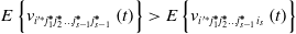
 \begin{equation} \min E\left\{\varphi _{{i}'j_{1}^{\boldsymbol{*}}j_{2}^{\boldsymbol{*}}\ldots j_{N}^{\boldsymbol{*}}}\left(t\right)\right\}\gt \max E\left\{\varphi _{{i}'{{j}_{1}}{j_{2}}\ldots {j_{{s}\mathit{-}\mathrm{1}}}}\left(t\right)\right\} \end{equation}
Among them,  $\varphi _{{i}'{{j}_{1}}{j_{2}}\ldots {j_{N}}}(t)$ represents other path (non-optimal) orientation values, and $\max (| j_{1}^{\boldsymbol{*}}-{j}_{1}| ,| j_{2}^{\boldsymbol{*}}-j_{2}| ,\ldots ,| j_{{s}\mathit{-}\mathrm{1}}^{\boldsymbol{*}}-j_{{s}\mathit{-}\mathrm{1}}| )\gt 0$.
3.2. Learning algorithm and convergence proof
3.2.1. Learning algorithm design
In both psychodynamics and biothermodynamics, a cognitive process can be regarded as a thermodynamic process that can be studied thermodynamically. Thermodynamic methods can be used to study it. Therefore, this paper combines a Monte Carlo-based simulated annealing algorithm to design a cognitive learning algorithm. A simulated annealing algorithm is a probabilistic algorithm with an approximate global optimum. According to the Metropolis criterion, the probability of reaching the equilibrium of energy in a particle at temperature T is  $\exp (\Delta{E})/K_{B}\ast T$. In the equation, E represents the internal energy of a particle at temperature T, $\Delta{E}$ is the variation of energy in a particle, and KB is the Boltzmann constant.
 \begin{equation} p\left(\alpha _{i'{j_{1}}{j_{2}}\ldots {j_{s-1}}}\left(t\right)\boldsymbol{|}s_{i}\left(t\right)\right) = \exp \left[\frac{\varphi _{i'{j_{1}}{j_{2}}\ldots {j_{s-1}}}\left(t+1\right)-\varphi _{i'{j_{1}}{j_{2}}\ldots {j_{s-1}}}\left(t\right)}{K_{B}T}\right] \end{equation}
Furthermore, suppose that the state of t is  $s_{i}(t)$, the operation behavior $\alpha _{i'{j_{1}}{j_{2}}\ldots {j_{s-1}}}$ is implemented and the state transition is t + 1 time state $s_{j}(t+1)$. According to Skinner’s OCR Theory, if the difference between the orientation values of state $s_{j}(t+1)$ and state $s_{i}(t)$ is $\varphi _{i'{j_{1}}{j_{2}}\ldots {j_{s\mathit{-}1}}}(t+1)-\varphi _{i'{j_{1}}{j_{2}}\ldots {j_{s\mathit{-}1}}}(t)\gt 0$, the probability $p(\alpha _{i'{j_{1}}{j_{2}}\ldots {j_{s-1}}}(t)\boldsymbol{|}s_{i}(t))$ of implementing operational behavior $\alpha _{i'{j_{1}}{j_{2}}\ldots {j_{s-1}}}$ in state $s_{i}(t)$ tends to increase in later learning and, vice versa, $\varphi _{i'{j_{1}}{j_{2}}\ldots {j_{s\mathit{-}1}}}(t+1)-\varphi _{i'{j_{1}}{j_{2}}\ldots {j_{s\mathit{-}1}}}(t)\lt 0$, the probability $p(\alpha _{i'{j_{1}}{j_{2}}\ldots {j_{s-1}}}(t)\boldsymbol{|}s_{i}(t))$ tends to decrease. Therefore, based on the idea of simulated annealing, the cognitive learning algorithm is designed as Eq. (8).
 \begin{equation} p\left(\alpha _{i'{j_{1}}{j_{2}}\ldots {j_{s-1}}}\left(t\right)\boldsymbol{|}s_{i}\left(t\right)\right) = \exp \left[\frac{\varphi _{i'{j_{1}}{j_{2}}\ldots {j_{s-1}}}\left(t+1\right)-\varphi _{i'{j_{1}}{j_{2}}\ldots {j_{s-1}}}\left(t\right)}{K_{B}T}\right] \end{equation}
When the generated random number  $\delta \in [\mathrm{0,1}]$ is less than $p(\alpha _{i'{j_{1}}{j_{2}}\ldots {j_{s-1}}}(t)\boldsymbol{|}s_{i}(t))$, the random action $\alpha _{i'{j_{1}}{j_{2}}\ldots {j_{s-1}}}$ is chosen, whereas the action with the largest orientation value is selected according to the strategy. The isometric cooling strategy is adopted to cool the temperature $T=\lambda _{_{T}}^{{n}}T_{0}$. The temperature decreases regularly, and the speed of change is slow. In the Equation, $T_{0}$ represents the initial temperature and n indicates the total number of iterations. $\lambda _{{_{T}}}$ is the value between [0,1]; the greater the value of $\lambda _{{_{T}}}$, the slower the annealing rate.
The implementation of the simulated annealing strategy is as follows:
Step 1: Initialization of initial temperature T and iteration number n;
Step 2: Acquires the state i of the current solution and generates a new state j;
Step 3: The random number  $\delta \in [\mathrm{0,1}]$ is generated, and the probability p of accepting the new solution j with the current solution i and temperature control parameter T is calculated according to Eq. (4). When $\delta \lt p$, accepting the new solution to the current problem is not acceptable.
Step 4: If the end condition is satisfied, the optimal solution is output; otherwise, Step 5 is executed.
Step 5: If each temperature T reaches n times, then according to the annealing strategy, the temperature T is cooled down to Step 1, and the temperature T after cooling is taken as the initial temperature of this learning; otherwise, the temperature T is changed to Step 2 to continue learning.
At the beginning of learning, the value of temperature T is larger and the probability of choosing a non-optimal solution is higher. With the increase in learning times and time itself, the value of temperature T becomes smaller and the probability of choosing the optimal solution increases. When  $T\rightarrow 0$, the non-optimal solution will not be selected and the global optimal solution will be found.
3.2.2. Proof of convergence of the learning algorithm
Suppose that the optimal path vector corresponding to the optimal path  $\phi _{{{i}'^{\mathit{*}}}j_{1}^{\boldsymbol{*}}j_{2}^{\boldsymbol{*}}\ldots j_{{s}\mathit{-}\mathrm{1}}^{\boldsymbol{*}}}$ is: $V_{{{i}'^{\mathit{*}}}j_{1}^{\boldsymbol{*}}j_{2}^{\boldsymbol{*}}\ldots j_{s-1}^{\boldsymbol{*}}}(t)=\{v_{{{i}'^{\mathit{*}}}j_{1}^{\boldsymbol{*}}j_{2}^{\boldsymbol{*}}\ldots j_{s-1}^{\boldsymbol{*}}1}(t)\mathrm{,}v_{{{i}'^{\mathit{*}}}j_{1}^{\boldsymbol{*}}j_{2}^{\boldsymbol{*}}\ldots j_{s-1}^{\boldsymbol{*}}2}(t)\mathrm{,}\ldots \mathrm{,}v_{{{i}'^{\mathit{*}}}j_{1}^{\boldsymbol{*}}j_{2}^{\boldsymbol{*}}\ldots j_{s-1}^{\boldsymbol{*}}r}(t)\}$.
Lemma 1: If the orientation value of each action in the orientation value vector is calculated by the reference Eq. (5), the following inequalities are satisfied for the optimal learning system  $\mathrm{CNM}_{{{i}'^{\mathit{*}}}j_{1}^{\boldsymbol{*}}j_{2}^{\boldsymbol{*}}\ldots j_{s-1}^{\boldsymbol{*}}}$:
 \begin{equation} E\left\{v_{{{i}'^{\mathit{*}}}j_{1}^{\boldsymbol{*}}j_{2}^{\boldsymbol{*}}\ldots j_{s-1}^{\boldsymbol{*}}}\left(t\right)\right\}\gt E\left\{v_{{{i}'^{\mathit{*}}}j_{1}^{\boldsymbol{*}}j_{2}^{\boldsymbol{*}}\ldots j_{s-2}^{\boldsymbol{*}}{i_{s}}}\left(t\right)\right\} \end{equation}
Among them,  ${i}'^{\mathit{*}} = 1,2,3; i_{s},j_{s\mathit{-}1}^{\boldsymbol{*}}=1,2,\ldots ,r\,\quad i_{s}\neq j_{s\mathit{-}1}^{\boldsymbol{*}}$.
Proof: In order to establish proof (8), we first give the following definition:
Definition 3: Assuming that the behavior path  $\phi _{{i}'{j_{1}}{j_{2}}\ldots {j_{{s}\mathit{-}\mathrm{1}}}}$ at time t is selected and the orientation value of the path $\varphi _{{i}'{j_{1}}{j_{2}}\ldots {j_{{s}\mathit{-}\mathrm{1}}}}$ is calculated from the feedback information of the system, the current orientation degree of path $\phi _{{i}'{j_{1}}{j_{2}}\ldots {j_{{s}\mathit{-}\mathrm{1}}}}$ is defined as: $u_{{i}'{j_{1}}{j_{2}}\ldots {j_{{s}\mathit{-}\mathrm{1}}}}(t)=\varphi _{{i}'{j_{1}}{j_{2}}\ldots {j_{{s}\mathit{-}\mathrm{1}}}}$, time t, and the current orientation value of other paths $\phi _{{i}''{i_{1}}{i_{2}}\ldots {i_{{s}-\mathrm{1}}}}$( $\exists k,i_{k}\neq j_{k}$) is defined as:
 \begin{equation} u_{{i}''{i_{1}}{i_{2}}\ldots {i_{{s}-\mathrm{1}}}}\left(t\right)=\varphi _{{i}''{i_{1}}{i_{2}}\ldots {i_{{s}-\mathrm{1}}}}\left(\tau _{{i}''{i_{1}}{i_{2}}\ldots {i_{{s}-\mathrm{1}}}}\right) \end{equation}
Among them,  $\tau _{{i}''{i_{1}}{i_{2}}\ldots {i_{{s}-\mathrm{1}}}}$ is the nearest time chosen by the path $\phi _{{i}''{i_{1}}{i_{2}}\ldots {i_{{s}-\mathrm{1}}}}$, and $\varphi _{{i}''{i_{1}}{i_{2}}\ldots {i_{{s}-\mathrm{1}}}}(\tau _{{i}''{i_{1}}{i_{2}}\ldots {i_{{s}-\mathrm{1}}}})$ indicates the orientation value of $\tau _{{i}''{i_{1}}{i_{2}}\ldots {i_{{s}-\mathrm{1}}}}$ time.
Remark 2: In layer s  $\mathrm{CNM}_{{i}'{j_{1}}{j_{2}}\ldots {j_{s-1}}}$ of the HS-CNM learning model, the orientation values of all the behaviors constitute vectors: $V_{{i}'{j_{1}}{j_{2}}\ldots {j_{s-1}}}(t)=\{v_{{i}'{j_{1}}{j_{2}}\ldots {j_{s-1}}1}(t),v_{{i}'{j_{1}}{j_{2}}\ldots {j_{s-1}}2}(t),\ldots ,v_{{i}'{j_{1}}{j_{2}}\ldots {j_{s-1}}r}(t)\}$. Each part of $V_{{j_{1}}{j_{2}}\ldots {j_{s-1}}}(t)$ is constructed as follows:
Layer s:
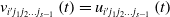 \begin{equation} v_{{i}'{j_{1}}{j_{2}}\ldots {j_{{s}\mathit{-}\mathrm{1}}}}\left(t\right)=u_{{i}'{j_{1}}{j_{2}}\ldots {j_{{s}-\mathrm{1}}}}\left(t\right) \end{equation}
Layer s−1:
 \begin{equation} v_{{i}'{j_{1}}{j_{2}}\ldots {j_{{s}\mathit{-}\mathrm{1}}}}\left({t}\right)=\max \left\{v_{{i}'{j_{1}}{j_{2}}\ldots {j_{{s}\mathit{-}\mathrm{1}}}1}\left({t}\right)\mathrm{,}v_{{i}'{j_{1}}{j_{2}}\ldots {j_{{s}\mathit{-}\mathrm{1}}}2}\left({t}\right)\mathrm{,}\ldots \mathrm{,}v_{{i}'{j_{1}}{j_{2}}\ldots {j_{{s}\mathit{-}\mathrm{1}}}r}\left({t}\right)\right\}\end{equation}
According to Eqs. (10) and (11), for the optimal learning system  $\mathrm{CNM}_{{{i}'^{\mathit{*}}}j_{1}^{\boldsymbol{*}}j_{2}^{\boldsymbol{*}}\ldots j_{{s}-1}^{\boldsymbol{*}}}$ at level s, the orientation value of the internal operation behavior satisfies:
 \begin{equation} E\{v_{{{i}'^{\mathit{*}}}j_{1}^{\boldsymbol{*}}j_{2}^{\boldsymbol{*}}\ldots j_{{s}-1}^{\boldsymbol{*}}{i_{s}}}(t)\}=E\{u_{{{i}'^{\mathit{*}}}j_{1}^{\boldsymbol{*}}j_{2}^{\boldsymbol{*}}\ldots j_{{s}-1}^{\boldsymbol{*}}{i_{s}}}(t)\}=E\{\varphi _{{{i}'^{\mathit{*}}}j_{1}^{\boldsymbol{*}}j_{2}^{\boldsymbol{*}}\ldots j_{{s}-1}^{\boldsymbol{*}}{i_{s}}}(\tau _{{{i}'^{\mathit{*}}}j_{1}^{\boldsymbol{*}}j_{2}^{\boldsymbol{*}}\ldots j_{s-1}^{\boldsymbol{*}}{i_{s}}})\} iN = 1,2,{\ldots}r \end{equation}
Eq. (13) can be obtained:
 \begin{equation} E\left\{v_{{{i}'^{\mathit{*}}}j_{1}^{\boldsymbol{*}}j_{2}^{\boldsymbol{*}}\ldots j_{{s}-1}^{\boldsymbol{*}}}\left(t\right)\right\}=E\left\{\varphi _{{{i}'^{\mathit{*}}}j_{1}^{\boldsymbol{*}}j_{2}^{\boldsymbol{*}}\ldots j_{{s}-1}^{\boldsymbol{*}}}\left(\tau _{{{i}'^{\mathit{*}}}j_{1}^{\boldsymbol{*}}j_{2}^{\boldsymbol{*}}\ldots j_{{s}-1}^{\boldsymbol{*}}}\right)\right\}\gt E\left\{\varphi _{{{i}'^{\mathit{*}}}j_{1}^{\boldsymbol{*}}j_{2}^{\boldsymbol{*}}\ldots j_{{s}-1}^{\boldsymbol{*}}{i_{s}}}\left(\tau _{{{i}'^{\mathit{*}}}j_{1}^{\boldsymbol{*}}j_{2}^{\boldsymbol{*}}\ldots j_{{s}-1}^{\boldsymbol{*}}{i_{s}}}\right)\right\}=E\left\{v_{{{i}'^{\mathit{*}}}j_{1}^{\boldsymbol{*}}j_{2}^{\boldsymbol{*}}\ldots j_{{s}-1}^{\boldsymbol{*}}{i_{s}}}\left(t\right)\right\} \end{equation}
Among them, i s = 1,2,…,r;  $i_{{s}}\neq j_{{s}\mathit{-}\textrm{1}}^{\boldsymbol{*}}$.
It can be seen from the cognitive model of the s level that the orientation value of the operation behavior is satisfied Eq. (8).
Next, we analyze the orientation value of the  $\mathrm{CNM}_{{{i}'^{\mathit{*}}}j_{1}^{\boldsymbol{*}}j_{2}^{\boldsymbol{*}}\ldots j_{{s}-2}^{\boldsymbol{*}}}$ operation behavior in the s-level optimal learning system, which can be obtained by Eqs. (8) and (14):
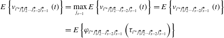 \begin{align} E\left\{v_{{{i}'^{\mathit{*}}}j_{1}^{\boldsymbol{*}}j_{2}^{\boldsymbol{*}}\ldots j_{{s}-2}^{\boldsymbol{*}}j_{s-1}^{\boldsymbol{*}}}\left(t\right)\right\} & =\max _{j_{s-1}}E\left\{v_{{{i}'^{\mathit{*}}}j_{1}^{\boldsymbol{*}}j_{2}^{\boldsymbol{*}}\ldots j_{{s}-2}^{\boldsymbol{*}}j_{s-1}^{\boldsymbol{*}}}\left(t\right)\right\}=E\left\{v_{{{i}'^{\mathit{*}}}j_{1}^{\boldsymbol{*}}j_{2}^{\boldsymbol{*}}\ldots j_{{s}-2}^{\boldsymbol{*}}j_{s-1}^{\boldsymbol{*}}}\left(t\right)\right\}\nonumber \\[5pt] & =E\left\{\varphi _{{{i}'^{\mathit{*}}}j_{1}^{\boldsymbol{*}}j_{2}^{\boldsymbol{*}}\ldots j_{{s}-2}^{\boldsymbol{*}}j_{s-1}^{\boldsymbol{*}}}\left(\tau _{{{i}'^{\mathit{*}}}j_{1}^{\boldsymbol{*}}j_{2}^{\boldsymbol{*}}\ldots j_{{s}-2}^{\boldsymbol{*}}j_{s-1}^{\boldsymbol{*}}}\right)\right\} \end{align}
 \begin{align} E\left\{v_{{{i}'^{\mathit{*}}}j_{1}^{\boldsymbol{*}}j_{2}^{\boldsymbol{*}}\ldots j_{{s}-2}^{\boldsymbol{*}}j_{s-2}^{\boldsymbol{*}}{i_{{s}-1}}}\left(t\right)\right\}&=\max _{l_{{s}}}E\left\{v_{{{i}'^{\mathit{*}}}j_{1}^{\boldsymbol{*}}j_{2}^{\boldsymbol{*}}\ldots j_{{s}-2}^{\boldsymbol{*}}j_{s-2}^{\boldsymbol{*}}{i_{{s}-1}}{l_{s}}}\left(t\right)\right\}=E\left\{v_{{{i}'^{\mathit{*}}}j_{1}^{\boldsymbol{*}}j_{2}^{\boldsymbol{*}}\ldots j_{{s}-2}^{\boldsymbol{*}}j_{s-2}^{\boldsymbol{*}}{i_{{s}-1}}{l_{s}}}\left(t\right)\right\}\nonumber \\[5pt] &=E\left\{\varphi _{{{i}'^{\mathit{*}}}j_{1}^{\boldsymbol{*}}j_{2}^{\boldsymbol{*}}\ldots j_{{s}-2}^{\boldsymbol{*}}j_{s-2}^{\boldsymbol{*}}{i_{{s}-1}}{l_{s}}}\left(\tau _{{{i}'^{\mathit{*}}}j_{1}^{\boldsymbol{*}}j_{2}^{\boldsymbol{*}}\ldots j_{{s}-2}^{\boldsymbol{*}}j_{s-2}^{\boldsymbol{*}}{i_{{s}-1}}{l_{s}}}\right)\right\} \end{align}
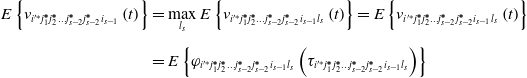
This can be obtained with Eqs. (15) and (16):
 \begin{align} E\left\{v_{{{i}'^{\mathit{*}}}j_{1}^{\boldsymbol{*}}j_{2}^{\boldsymbol{*}}\ldots j_{{s}-2}^{\boldsymbol{*}}j_{s-1}^{\boldsymbol{*}}}\left(t\right)\right\}&=E\left\{\varphi _{{{i}'^{\mathit{*}}}j_{1}^{\boldsymbol{*}}j_{2}^{\boldsymbol{*}}\ldots j_{{s}-2}^{\boldsymbol{*}}j_{s-1}^{\boldsymbol{*}}}\left(\tau _{{{i}'^{\mathit{*}}}j_{1}^{\boldsymbol{*}}j_{2}^{\boldsymbol{*}}\ldots j_{{s}-2}^{\boldsymbol{*}}j_{s-1}^{\boldsymbol{*}}}\right)\right\}\nonumber \\[5pt] & \gt E\left\{v_{{{i}'^{\mathit{*}}}j_{1}^{\boldsymbol{*}}j_{2}^{\boldsymbol{*}}\ldots j_{{s}-2}^{\boldsymbol{*}}j_{s-2}^{\boldsymbol{*}}{i_{{s}-1}}}\left(t\right)\right\}=E\left\{\varphi _{{{i}'^{\mathit{*}}}j_{1}^{\boldsymbol{*}}j_{2}^{\boldsymbol{*}}\ldots j_{{s}-2}^{\boldsymbol{*}}j_{s-2}^{\boldsymbol{*}}{i_{{s}-1}}{l_{s}}}\left(\tau _{{{i}'^{\mathit{*}}}j_{1}^{\boldsymbol{*}}j_{2}^{\boldsymbol{*}}\ldots j_{{s}-2}^{\boldsymbol{*}}j_{s-2}^{\boldsymbol{*}}{i_{{s}-1}}{l_{s}}}\right)\right\} \end{align}
where, l s, j s-1 = 1,2,…,r;i s 1 = 1,2,…,r; $i_{{s}-1}\neq j_{{s}-2}^{\boldsymbol{*}}$.
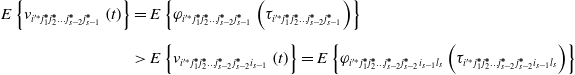
Following the same steps, we can obtain the following conclusions:
 \begin{equation} E\left\{v_{{{i}'^{\mathit{*}}}j_{1}^{\boldsymbol{*}}j_{2}^{\boldsymbol{*}}\ldots j_{s-1}^{\boldsymbol{*}}j_{s\mathit{-}1}^{\boldsymbol{*}}}\left(t\right)\right\}\gt E\left\{v_{{{i}'^{\mathit{*}}}j_{1}^{\boldsymbol{*}}j_{2}^{\boldsymbol{*}}\ldots j_{s-1}^{\boldsymbol{*}}{i_{s}}}\left(t\right)\right\} \end{equation}
where, i s-1 = 1,2,…,r; $i_{s}\neq j_{s\mathit{-}1}^{\boldsymbol{*}}$, and lemma is proved.
Theorem 1: When the probability of the operation satisfies  $0\lt p_{{i}'{j_{1}}{j_{2}}\ldots {j_{{s}-\mathrm{1}}}}\lt 1$, the optimal path $\phi _{{{i}'^{\mathit{*}}}j_{1}^{\boldsymbol{*}}j_{2}^{\boldsymbol{*}}\ldots j_{{s}\mathit{-}1}^{\boldsymbol{*}}}$ is selected according to probability $q_{{i}'{j_{1}}{j_{2}}\ldots {j_{{s}-\mathrm{1}}}}(t)\approx 1$.
It has been proven that the probability of the operation behavior is satisfied:  $p_{\boldsymbol{\min }}\leq p_{{i}'{j_{1}}{j_{2}}\ldots {j_{{s}-\mathrm{1}}}}\leq p_{\boldsymbol{\max }}$, where pmax is close to 1 and pmax is close to 0. From lemma 1, it can be seen that the orientation value corresponding to the optimal operation behavior is also the largest, so the occurrence probability of the operation behavior corresponding to the optimal action path is satisfied: $\lim _{t\rightarrow \infty }p_{{{i}'^{\mathit{*}}}j_{1}^{\boldsymbol{*}}j_{2}^{\boldsymbol{*}}\ldots j_{{s}\mathit{-}1}^{\boldsymbol{*}}}=p_{\boldsymbol{\max }}$. Then, the probability corresponding to the optimal action path is satisfied:
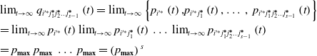 \begin{equation} \begin{array}{l} \lim _{t\rightarrow \infty }q_{{{i}'^{\mathit{*}}}j_{1}^{\boldsymbol{*}}j_{2}^{\boldsymbol{*}}\ldots j_{{s}\mathit{-}1}^{\boldsymbol{*}}}\left(t\right)=\lim _{t\rightarrow \infty }\left\{p_{{{i}'^{\mathit{*}}}}\left(t\right)\mathrm{,}p_{{{i}'^{\mathit{*}}}j_{1}^{\boldsymbol{*}}}\left(t\right)\mathrm{,}\ldots \,\mathrm{,}\,\,p_{{{i}'^{\mathit{*}}}j_{1}^{\boldsymbol{*}}j_{2}^{\boldsymbol{*}}\ldots j_{{s}\mathit{-}1}^{\boldsymbol{*}}}\left(t\right)\right\}\\[5pt] =\lim _{t\rightarrow \infty }p_{{{i}'^{\mathit{*}}}}\left(t\right)\lim _{t\rightarrow \infty }p_{{{i}'^{\mathit{*}}}j_{1}^{\boldsymbol{*}}}\left(t\right)\,\ldots \,\lim _{t\rightarrow \infty }p_{{{i}'^{\mathit{*}}}j_{1}^{\boldsymbol{*}}j_{2}^{\boldsymbol{*}}\ldots j_{{s}\mathit{-}1}^{\boldsymbol{*}}}\left(t\right)\\[5pt] =p_{\boldsymbol{\max }}\,p_{\boldsymbol{\max }}\,\ldots \,p_{\boldsymbol{\max }}=\left(p_{\boldsymbol{\max }}\right)\,^{\mathit{\!\!s}} \end{array} \end{equation}
This can be obtained with type Eqs. (15) and (16), that Eq. (18) is  $\lim _{t\rightarrow \infty }q_{{{i}'^{\mathit{*}}}j_{1}^{\boldsymbol{*}}j_{2}^{\boldsymbol{*}}\ldots j_{{s}\mathit{-}1}^{\boldsymbol{*}}}(t)\approx 1$, the theorem is proved.
4. Realization of robot autonomous navigation
4.1. Robot State and Behavior Classification
4.1.1. Sub-task status division
The purpose of the robot path planning is to make the robot reach the target point safely and without collisions, having departed from the starting point. It is necessary to consider the distance information of the obstacles, as well as the movement state and the position and distance information of the target point. These changing pieces of environmental information constitute a large state space, which seriously affects the learning efficiency of the robot. According to the hierarchical and abstract strategy of the hierarchical cognitive model, the path planning task of a mobile robot is divided into three basic sub-tasks  $S=\{S_{1}, S_{2}, S_{3}\}$: static obstacle avoidance, dynamic obstacle avoidance, and moving toward the target point. The state space is divided into three small-scale spaces in order to improve the learning efficiency of the robot.
Assuming that the robot can turn freely in a narrow environment without touching any obstacles, the radius of rotation of the robot is not considered in the navigation algorithm, and the robot is simplified to a particle. The relationship between robots, obstacles, and target points is shown in Fig. 2.
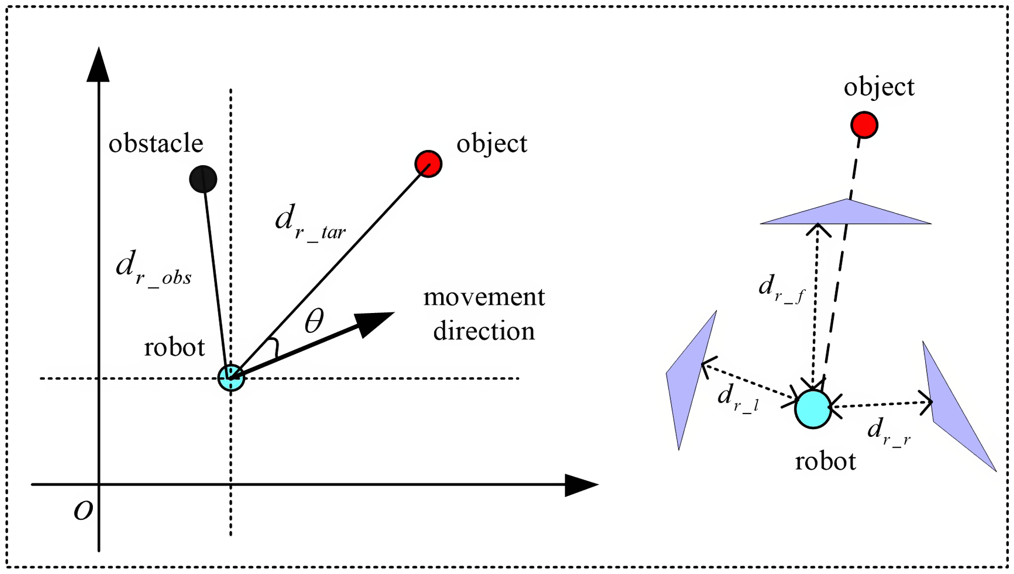
Figure 2. The relationship between robots, obstacles, and target points.
The environmental information around the mobile robot is mainly detected by the camera. In order to simplify the problem, the detection range of the sensor is divided into three areas: left, front, and right. Thus, the environmental state between the robot and the obstacle can be expressed through distance information in three directions. In addition, we do not pay attention to the specific location information and determine the distance of the robot itself and all the obstacles, but rather only to the approximate distance range and relative position direction of the nearest obstacle. Based on this, we define the state space of the three sub-tasks.
Definition 4: The static obstacle avoidance task mainly considers the robot moving towards the target point while avoiding obstacles. Therefore, the minimum distance measurements of static obstacles in three areas detected by sensors, the angle between the moving direction of the mobile robot and the direction of target point, and the distance between the mobile robot and the target point are taken as the input state information of the static obstacle avoidance sub-task module:
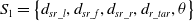 \begin{equation} S_{1}=\left\{d_{sr\boldsymbol{\_ }l},d_{sr\boldsymbol{\_ }f},d_{sr\boldsymbol{\_ }r},d_{r\boldsymbol{\_ }tar},\theta \right\} \end{equation}
In the Eq. (20),  $d_{sr\boldsymbol{\_ }l}$ is the distance from the left side of the robot to the static obstacle; $d_{{\boldsymbol{{s}}}r\boldsymbol{\_ }f}$ is the distance between the front and the static obstacles of the robot; $d_{sr\boldsymbol{\_ }r}$ is the distance from the right side of the robot to the static obstacle; $d_{r\boldsymbol{\_ }tar}$ is the distance between robots and target points; and $\theta$ is the angle between the moving direction and the target point of the robot.
The distance from static obstacles in three directions is discretized into N (Near) and F (Far), as shown in Eq. (21).
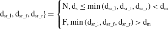 \begin{equation}\mathrm{d}_{\mathrm{sr}\_ \mathrm{l}},\mathrm{d}_{\mathrm{sr}\_ \mathrm{f}},\mathrm{d}_{\mathrm{sr}\_ \mathrm{r}}\}=\begin{cases} \mathrm{N},\mathrm{d}_{\mathrm{s}}\leq \min (\mathrm{d}_{\mathrm{sr}\_ \mathrm{l}},\mathrm{d}_{\mathrm{sr}\_ \mathrm{f}},\mathrm{d}_{\mathrm{sr}\_ \mathrm{r}})\lt \mathrm{d}_{\mathrm{m}}\\[5pt] \mathrm{F},\min (\mathrm{d}_{\mathrm{sr}\_ \mathrm{l}},\mathrm{d}_{\mathrm{sr}\_ \mathrm{f}},\mathrm{d}_{\mathrm{sr}\_ \mathrm{r}})\gt \mathrm{d}_{\mathrm{m}} \end{cases}\end{equation} $\mathrm{d}_{\mathrm{s}}$ represents the minimum dangerous distance, when any detection distance is less than $\mathrm{d}_{\mathrm{s}}$ represents the mobile robot obstacle avoidance failure. $\mathrm{d}_{\mathrm{m}}$ represents the maximum safe distance, and the robot can walk safely at the maximum speed when the detection distance in all directions is greater than $\mathrm{d}_{\mathrm{m}}$.
The distance between the robot and the target point is also discretized into N and F, and the angle between the direction of motion and the target point is discretized into zero and non-zero, {zero, not zero}.
Definition 5: The dynamic obstacle avoidance task mainly considers avoiding dynamic obstacles while avoiding collisions with static obstacles. Therefore, the minimum distance measurements of obstacles in three areas detected by sensors, the moving direction of dynamic obstacles, and the location information of dynamic obstacles are taken as the input state information of the dynamic obstacle avoidance sub-task module:
 \begin{equation} S_{2}=\left\{d_{sr\boldsymbol{\_ }l},d_{sr\boldsymbol{\_ }f},d_{sr\boldsymbol{\_ }r},d_{\boldsymbol{d}r\boldsymbol{\_ }l},d_{dr\boldsymbol{\_ }f},d_{dr\boldsymbol{\_ }r},\theta _{d}\right\} \end{equation}
In the Eq. (22),  $d_{\boldsymbol{d}r\boldsymbol{\_ }l}$ is the distance from the left side of the robot to the dynamic obstacle; $d_{dr\boldsymbol{\_ }f}$is the distance from the front of the robot to the dynamic obstacles; $d_{dr\boldsymbol{\_ }r}$ is the distance from the right side of the robot to the dynamic obstacles; and $\theta _{\boldsymbol{d}}$ is the angle between the direction of motion of a robot and the direction of motion of a moving obstacle.
The distance from the dynamic obstacle in three directions is also discretized into n (Near) and F (Far) whose form is the same as Eq. (21).
A virtual rectangular coordinate system is established, with the robot as the origin, and the direction of the robot’s motion and the dynamic obstacle are used as the x-axis, as shown in Fig. 3.
The angle between the robot motion direction and the dynamic obstacle movement direction is discretized as Eq. (23).
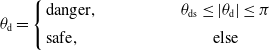 \begin{equation} \theta _{\mathrm{d}}=\left\{\begin{array}{l} \text{danger},\enspace \enspace \enspace \enspace \enspace \enspace \enspace \enspace \enspace \enspace \theta _{\mathrm{ds}}\leq \left| \theta _{\mathrm{d}}\right| \leq \pi \\[5pt] \mathrm{safe},\enspace \enspace \enspace \enspace \enspace \enspace \enspace \enspace \enspace \enspace \enspace \enspace \quad \quad \mathrm{else} \end{array}\right. \end{equation}
In Eq. (23),  $\theta _{ds}$ represents the minimum risk angle.
Definition 6: A target-oriented task mainly considers the way in which a robot can move radially towards a target point along an optimal path. Therefore, the distance between the mobile robot and the target point, and the angle between the direction of the mobile robot and the direction of the target point are taken as the input state information of the sub-task module of the target-oriented task:
 \begin{equation} S_{3}=\left\{d_{r\boldsymbol{\_ }tar},\theta \right\} \end{equation}
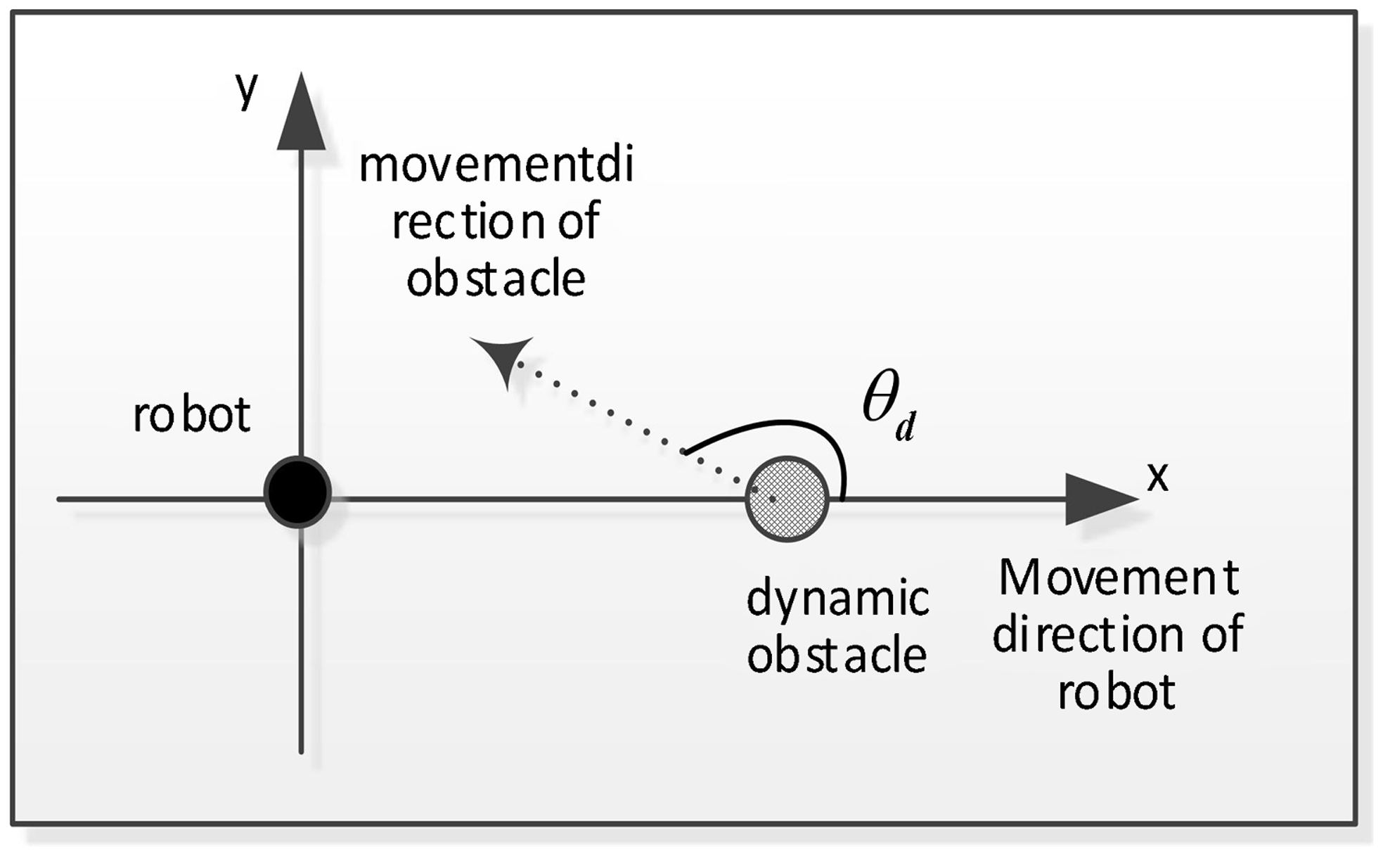
Figure 3. Virtual rectangular coordinate system.
The form of discretization is the same as in Definition 5.
4.1.2. Sub-task status division
The control variables of the robot are linear speed  $v$ and robot motion angle ${\Delta}\theta$. In the robot behavior control structure, the goal of obstacle avoidance and orientation can be achieved by determining the appropriate $v$ and ${\Delta}\theta$. Therefore, $v_{i}$ and ${\Delta}\theta$ are the behavior a of the robot.
 \begin{equation} a=\left\{v,{\Delta} \theta \right\} \end{equation}
When performing path planning tasks, the robot operation as follows:
If the robot is far from the static and dynamic obstacles, then the robot can directly navigate to the target at its maximum speed and perform the sub-task of moving toward the target.
If there are static obstacles near the robot, the robot tries to move left or right along the nearest obstacle in the direction of the target; that is, moving along the left or right static obstacles to perform the static obstacle avoidance task.
If there are dynamic obstacles near the robot, the robot tries to move left or right along the nearest dynamic obstacle, that is moving along the left or right dynamic obstacle to perform the dynamic obstacle avoidance task.
Considering that the behavior of the sub-task selection layer is roughly divided, all sub-tasks adopt the same behavior set  $A_{1}=A_{2}=A_{3}=\{a_{1},a_{2},a_{3}\}$.
Remark 3: The behavior set A of the robot in the sub-task selection layer is:
 \begin{equation} A_{1}=A_{2}=A_{3}=\left\{a_{1},a_{2},a_{3}\right\} \end{equation} $a_{1}$: The robot rotates $+20^{\circ }$ and advances 100 mm. $a_{2}$: The robot rotates $-20^{\circ }$ and advances 100 mm. $a_{3}$: The robot advances 200 mm.
+: Clockwise rotation. -:Counterclockwise rotation.
The behavior of the coarse selection of the sub-task selection layer is refined by one level.
Remark 4: The behavior refinement layer set is shown in Table I.
4.2. Three-dimensional simulation experiment
4.2.1. Test environment and parameter settings
The computer operating environment settings for all the simulation experiment are as follows: the computer processor is Intel(R) Core(TM) i7-4790, the computer frequency of 3.6 GHz, and the computer RAM is 8 GB. The simulation software adopts MobotSim in this paper. A three-dimensional simulation experiment is carried out based on the software platform. The robot is approximately circular, with a diameter of 0.5 m. The robot is marked in red, and the target point is a smaller yellow circle, as shown in Fig. 4. There are obstacles in the environment: five in total from the starting point to the destination. The shapes and sizes of the obstacles are different. Three obstacles surround the robot in three directions and the other two obstacles surround the destination in two directions. The starting position of the robot is in the lower left corner of the environment, and the target is located in the upper right corner of the environment. The time interval of the time step is 0.1 s, and the speed of the robot center is 0.2 m/s. The mobile robot system can detect the distance of obstacles in different directions through detection devices and can sense the current location and target location information. It can then avoid obstacles through autonomous learning, and find the best or a better path through which to reach the target point.
Table I. Layer thinning behavior set.
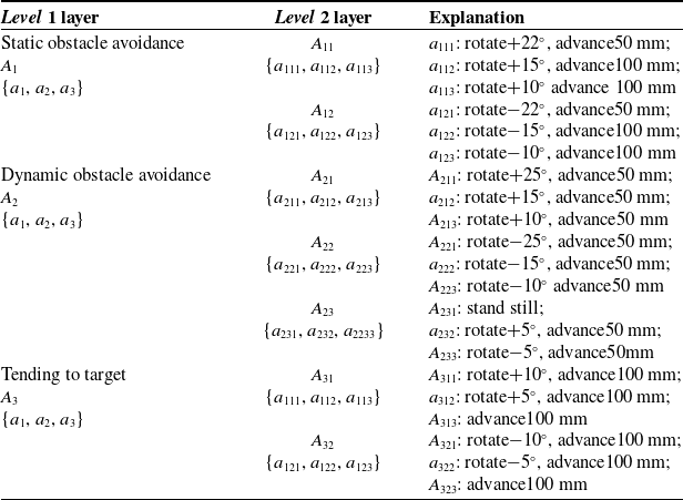
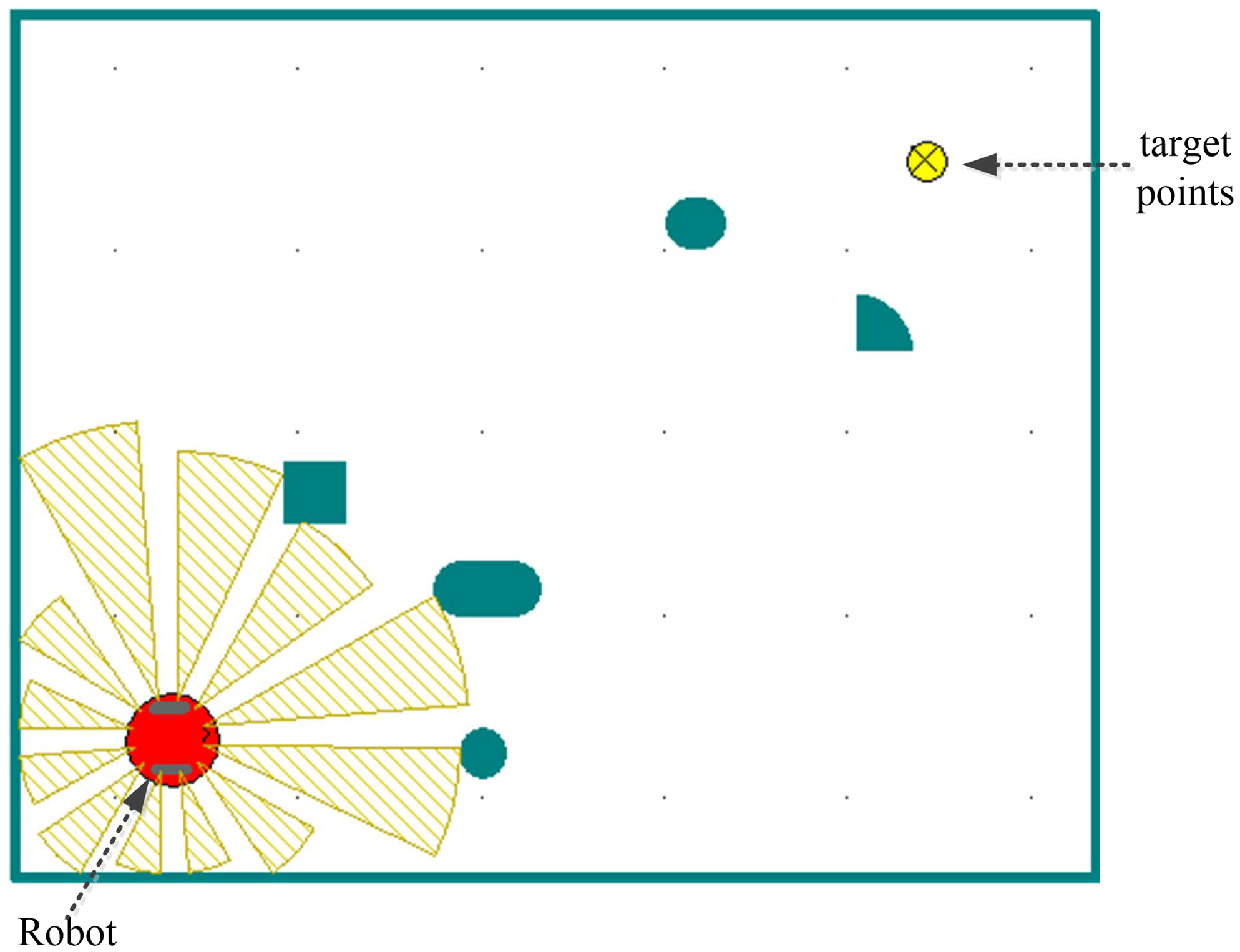
Figure 4. 2D simulation environment.
The initial conditions of the experiment are as follows: In the probability renewal Eq. (4), the initial temperature  $K_{B}T$ = 10,000, the cooling coefficient $\lambda _{{_{T}}} = 0\boldsymbol{.}9$; the minimum dangerous distance $d_{s}$ = 0.1 m, the maximum safe distance $d_{m}$ = 0.9m; the maximum speed $V_{\max }$ = 0.15 m/s; and the initial selection probability of each action in the behavior set is the same.
4.2.2. Experimental results and analysis
First, in the static obstacle environment, the feasibility of autonomous learning ability of cognitive model based on operational conditioned reflex and hierarchical structure is tested. Figure 5 shows the simulation results of path planning in a static environment. Figure 5 shows the simulation result of path planning in a static environment. From the results of the first round of experiments, it can be seen that the robot has not yet learned and has not accumulated enough knowledge about the environment. Therefore, the path appears to be more chaotic. Several failed attempts were made, in which the robot collided with obstacles but, after a period of exploration and further attempts, the robot can solve the predicament and continue to move toward the destination. The results of the second round of experiments show that the number of collisions is reduced, and the time it takes to solve the problem is shortened after the collisions occur. This shows that, after cognitive learning, the robot has a certain level of environmental experience. From the results of the third round of experiments, we can see that the robot has learned a relatively optimal path without collision. This shows that, after three rounds of experiments, the robot has grasped the general situation of the starting point, end point, and distribution of obstacles and can make a relatively stable judgment. The results of the follow-up experiments also show that the robot’s judgment of the route has been amended, indicating that the model converges and the learning is over. Experiment results shown in Fig. 5 depict the way in which the trained mobile robot can reach the target point from the starting point without collisions and find an almost optimal path.
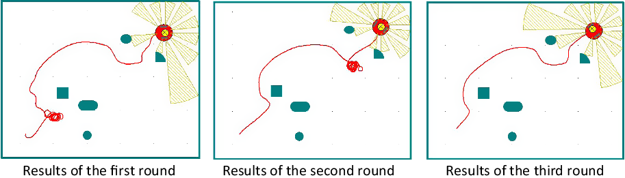
Figure 5. Results of the three-dimensional simulation experiments.
From Definitions 1 and 2, we can know the behavior path and behavior path selection probability. The histogram shown in Fig. 6 depicts the evolution process of each behavior probability. From the simulation results shown in Fig. 6, it can be seen that, at the end of the first round of learning, the probability values of each behavior are no longer equal, but a gap is not obvious. When the second round of learning is carried out, the probability of one behavior occurring continues to increase, while the probability of other behaviors occurring gradually decreases. After three rounds of learning, the probability of one behavior occurring is close to 1, while the probability of other behaviors is close to 0. This shows that robots have learned to choose the most favorable behavior for themselves by learning and starting to choose behavior autonomously.
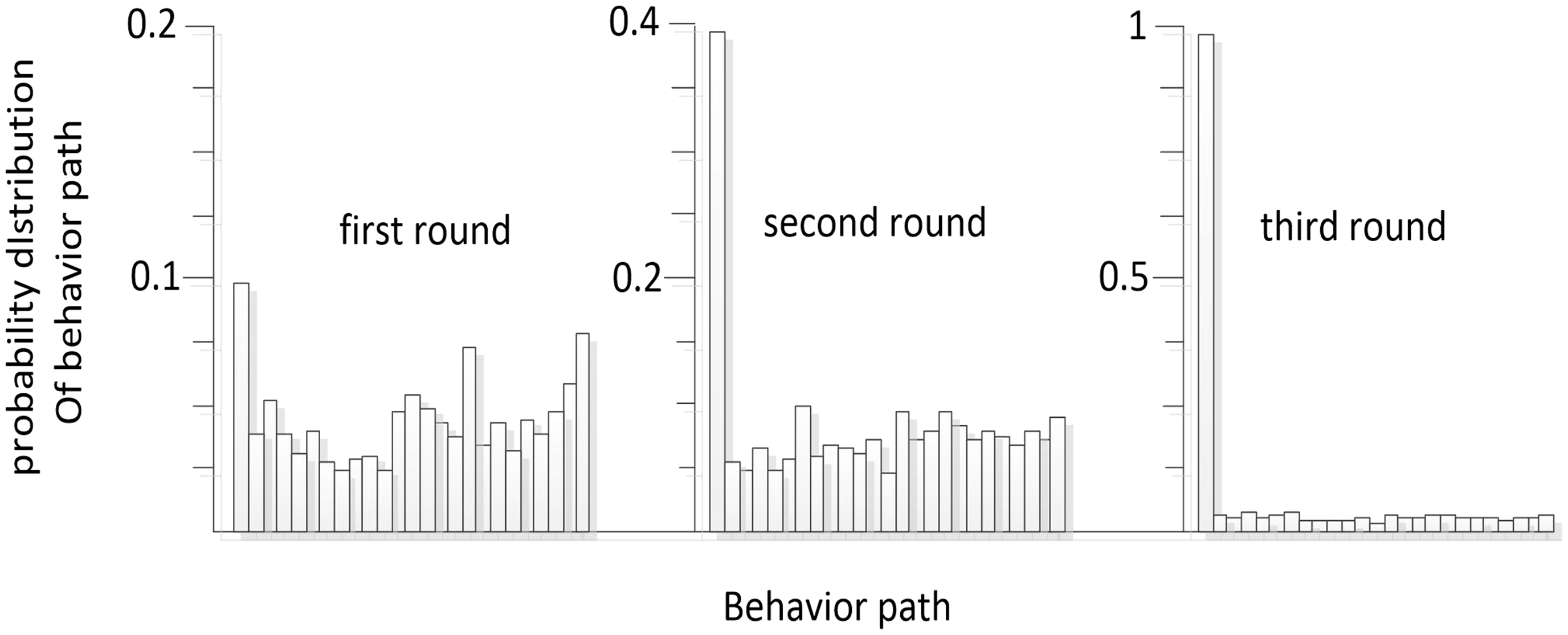
Figure 6. Probability evolution process of the static obstacle avoidance behavior path.
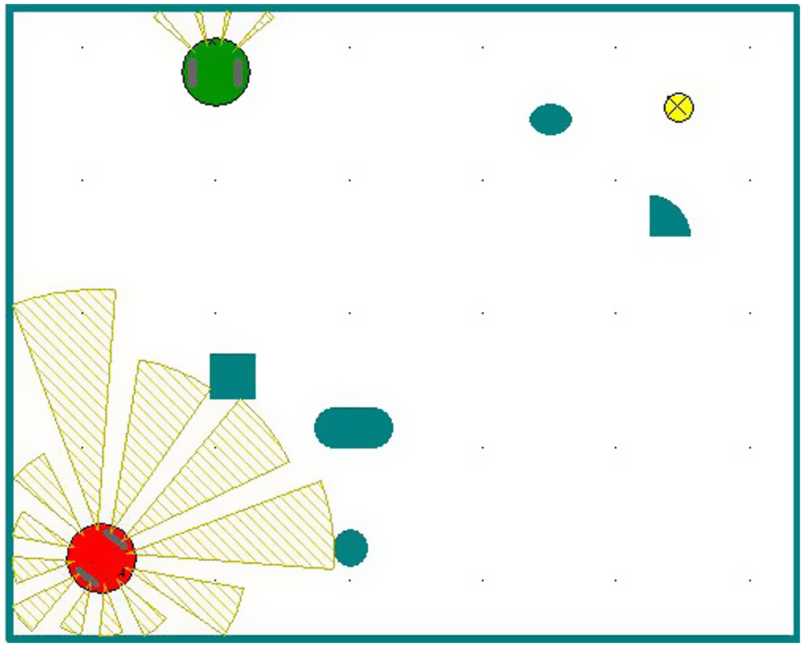
Figure 7. Environment after adding dynamic obstacles.
Changing the environmental information, adding a dynamic obstacle, and replacing it with a robot moving at a uniform speed v, as shown in Fig. 7, means that the best behavior learned before is no longer adapted to the new environment. Due to the complexity of environmental information, the robot needs to explore more. Therefore, the cooling coefficient is greatly increased  $\lambda _{{_{T}}} = 0\boldsymbol{.}95$, slowing down the cooling rate and increasing the randomness of the robot action selection at the initial stage of training. Because the randomness of action selection is increased, the success rate is low in the initial stages. After four rounds of learning, the optimal path is acquired. Figure 8 is the result of the fourth round of learning. As can be seen in the graph, when the robot is about to reach point A, the sub-task of avoiding dynamic obstacles is selected to avoid collision with dynamic obstacles at point A. After reaching point B, the dynamic obstacle avoidance sub-task is completed. The static obstacle avoidance sub-task is selected again according to the environmental state. The robot is in a safe environment at point C. Therefore, the static obstacle avoidance sub-task is ended and the sub-task tending to the target point is selected. The histogram shown in Fig. 9 shows the evolutionary process of each behavior probability. After the fourth round of learning, the robot has learned the new optimal behavior. Compared to the experimental results shown in Figs. 5 and 6, the hierarchical model designed has a certain generalization ability for the autonomous path planning of robots. Comparing Figs. 6 and 9, it can be seen that without dynamic obstacles, the robot converges after three rounds of learning, and after adding dynamic obstacles, the robot converges after four rounds of learning. This shows even if the environmental information changes, the learning convergence speed does not decrease significantly and the robots can adapt to the environment quickly and rediscover the rules, which show the learning ability and adaptability similar to animals and can solve the dimensionality disaster problem in a complex environment.
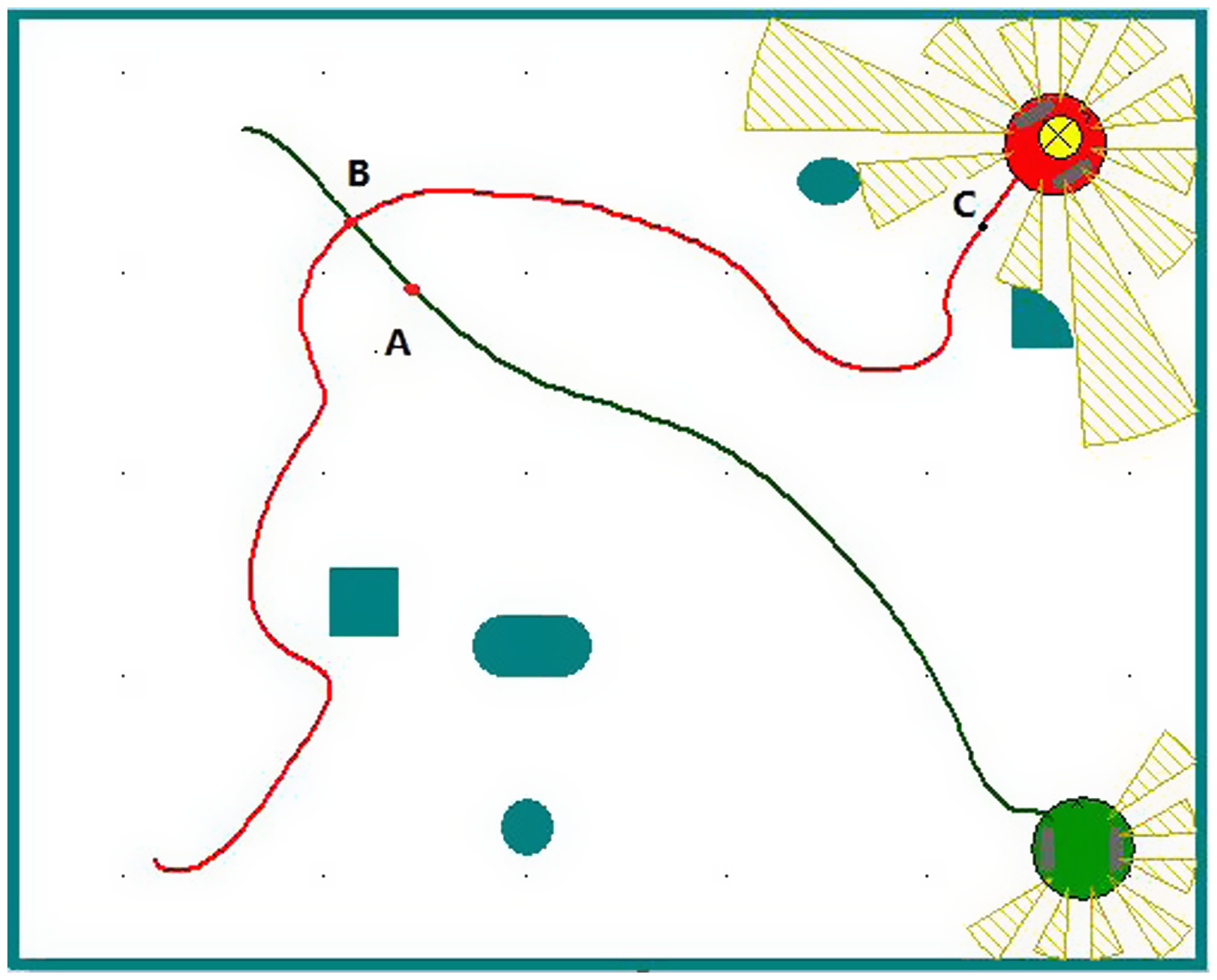
Figure 8. Dynamic obstacle avoidance path.
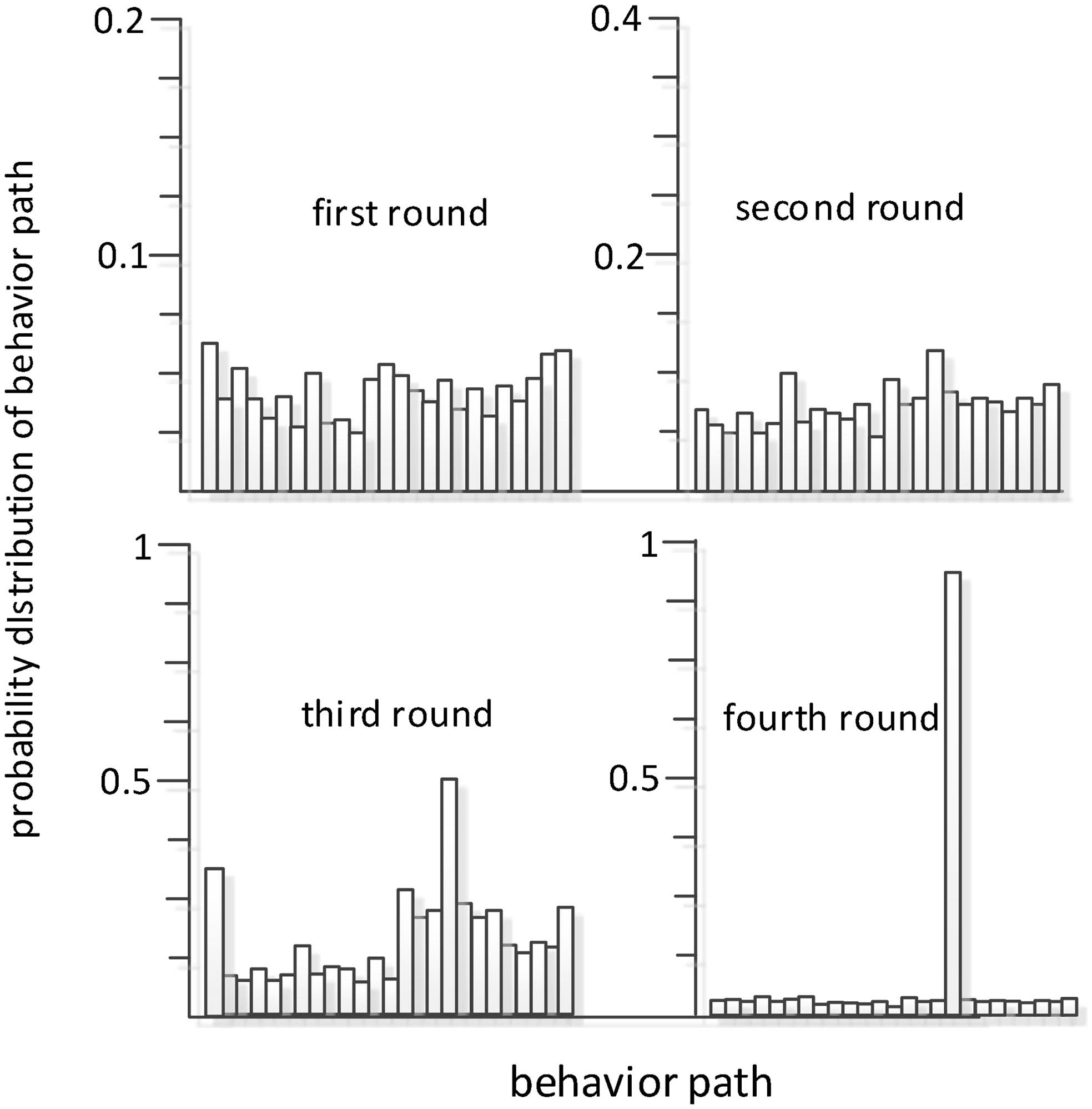
Figure 9. Probabilistic evolution process of the dynamic obstacle avoidance behavior path.
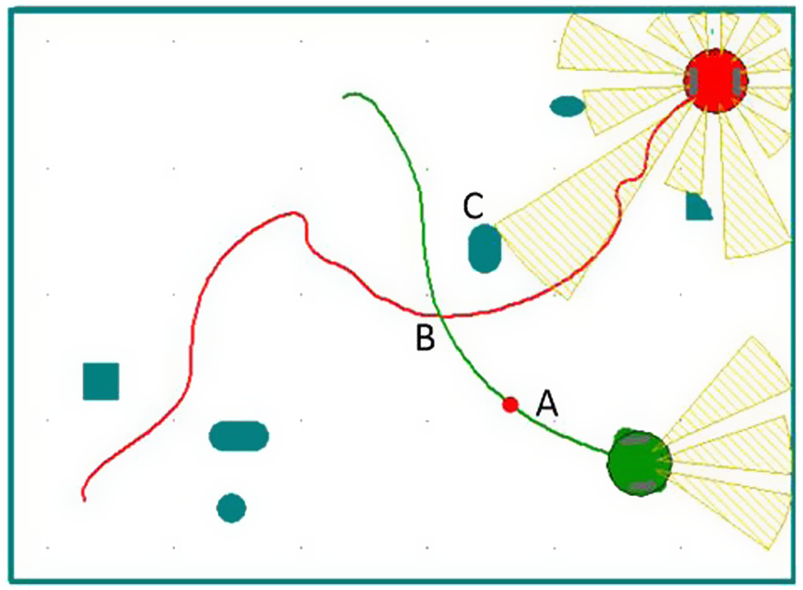
Figure 10. Autonomous navigation results facing dynamic and static obstacles.
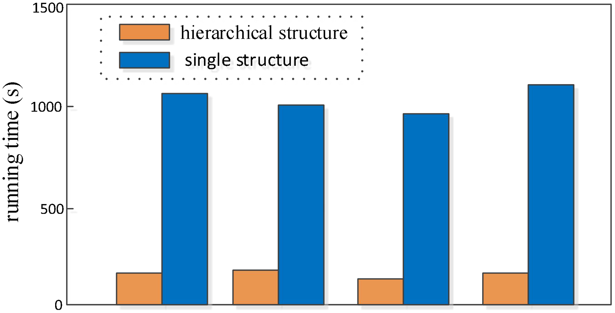
Figure 11. The comparison of running time on hierarchical structure and single structure.
In order to further test the autonomous navigation performance of the robot, the experiment that the robot faces both dynamic and static obstacles when it meets with dynamic obstacles is added. As shown in Fig. 10, the experimental results show that the robot encounters dynamic obstacles at point A and static obstacles at point C at point B, and the robot can avoid dynamic and static obstacles at the same time and successfully reach the target point.
In order to prove the rapidity of the hierarchical cognitive model, the results are compared with the single cognitive model. We can see that the probability of successful navigation is 80% by using single structure based on twenty times experiments; however, the hierarchical structure is about 94%. The results of four times successful navigation were extracted from the experimental results, and their running times were compared as shown in Fig. 11.
According to the above experiments, it can be concluded that although the cognitive model of single structure can successfully realize robot autonomous navigation, its convergence speed is much slower than that of hierarchical structure. From the practical point of view, the hierarchical structure is better than the single structure.
In order to further prove the validity of the design model HCNM, we compared it with the similar hierarchical reinforcement learning model (HRLM). The similarity between the two models is that they are hierarchical, reward-based, "trial-and-error" learning. The difference is that the learning information of Q-learning which is the main algorithm reinforcement learning is stored in the Q table, which needs to update continuously. However, the learning algorithm of this paper can obtain autonomously the environmental information. The experimental results are shown in Figs. 12 and 13.
When the robot can navigate to the target point autonomously, it represents convergence. The time from the beginning of robot navigation to the end of navigation is the convergence time. Figures 12 and 13 show that HCNM is better than HRLM both in experimental effects and convergence time. The final path of HCNM model is clearer, and the effect is better. From the point of view of convergence speed, the convergence time of the HCNM is significantly reduced, which indicates that the convergence speed of HCNM is faster than HRLM. In addition, in this experiment, there are obstacles on the three sides of the target point, which increase the difficulty of navigation. The results show that the robot can successfully reach the target point through autonomous learning.
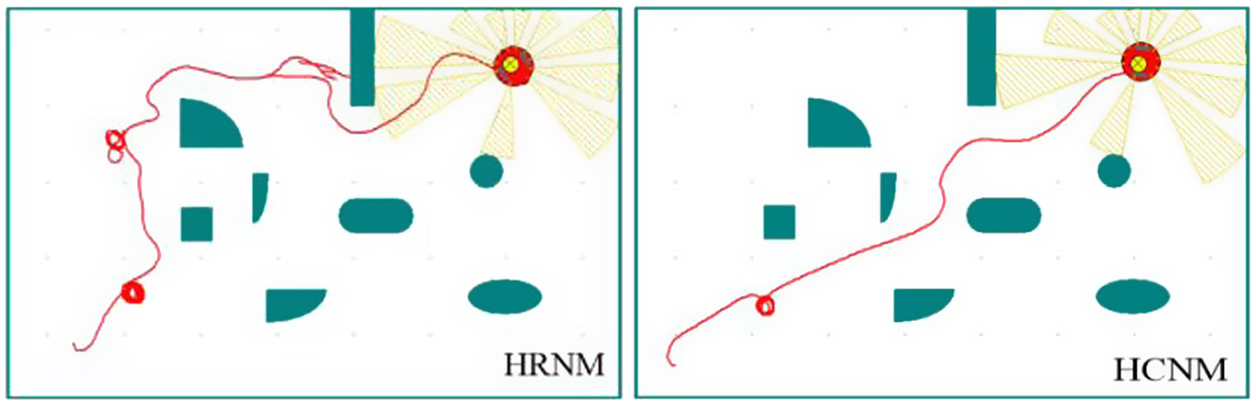
Figure 12. The navigation of HCNM and HRLM model.
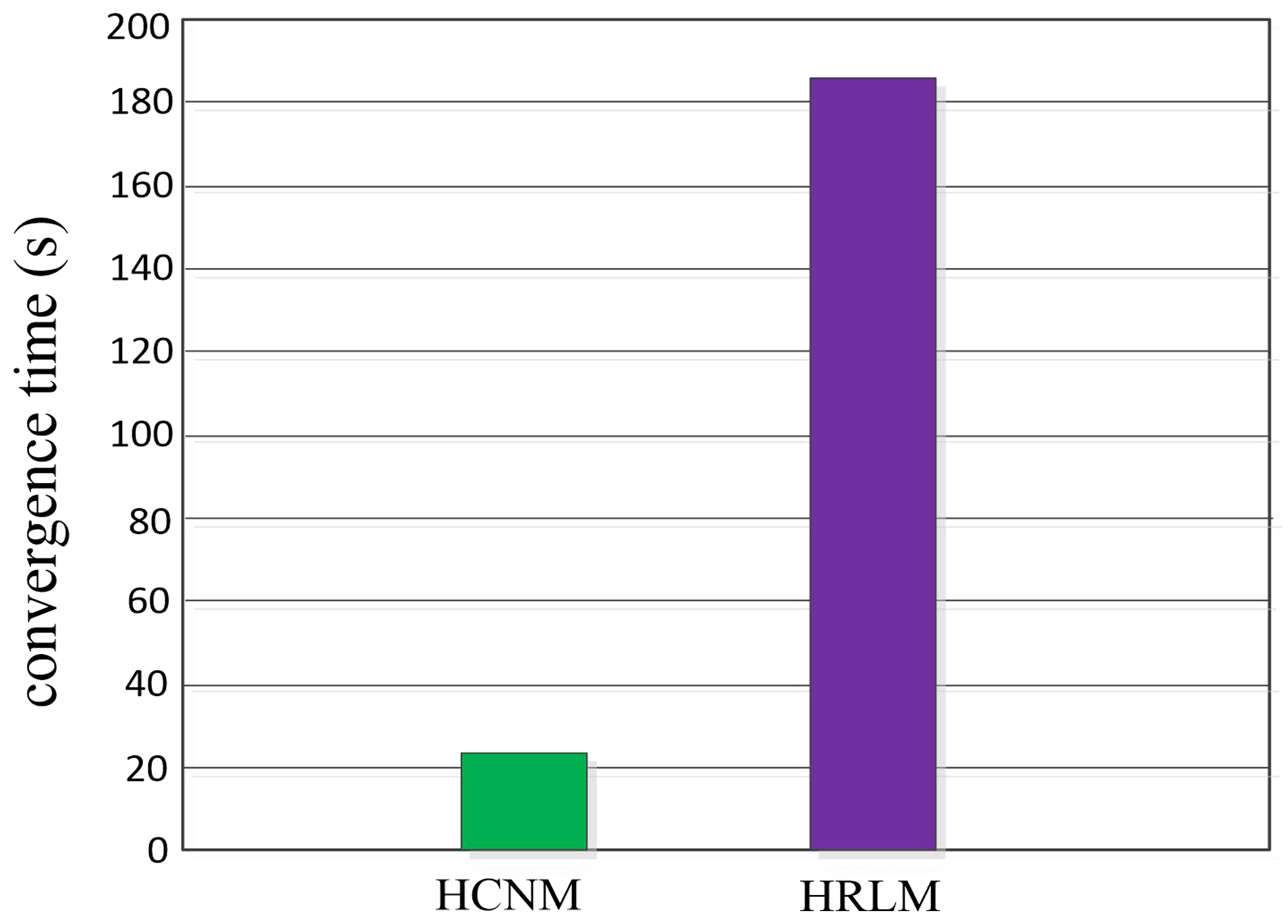
Figure 13. The convergence time of two models.
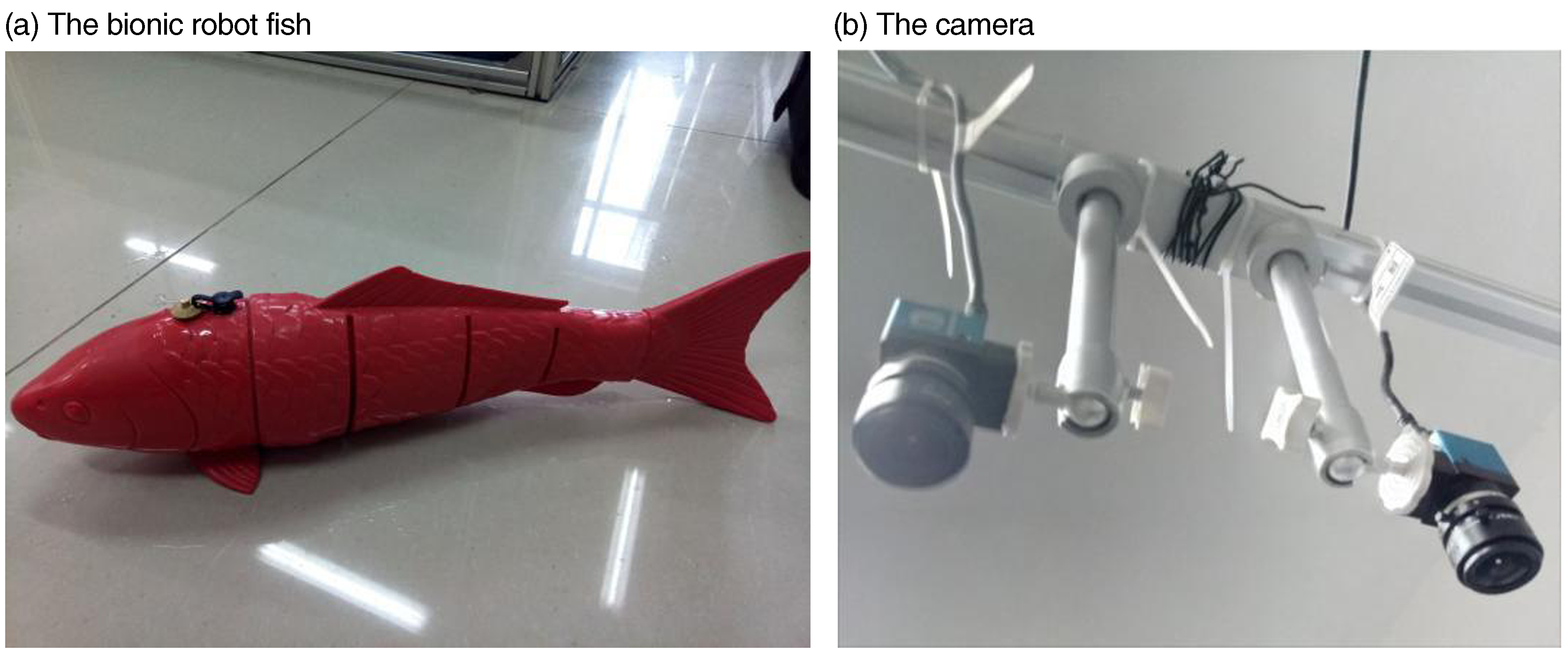
Figure 14. Experimental system of a bionic robot fish.
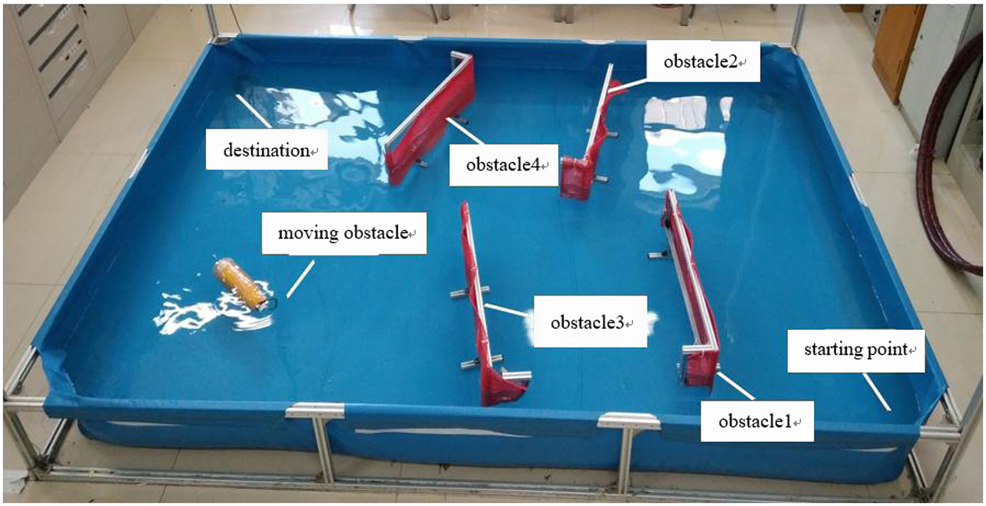
Figure 15. Top view of the experimental environment.
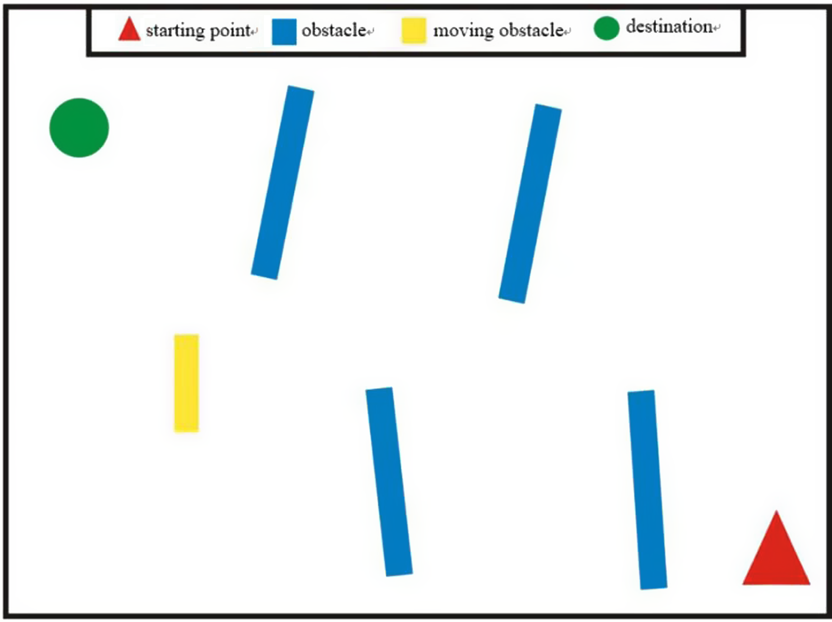
Figure 16. Schematic diagram of the experimental environment simulation.
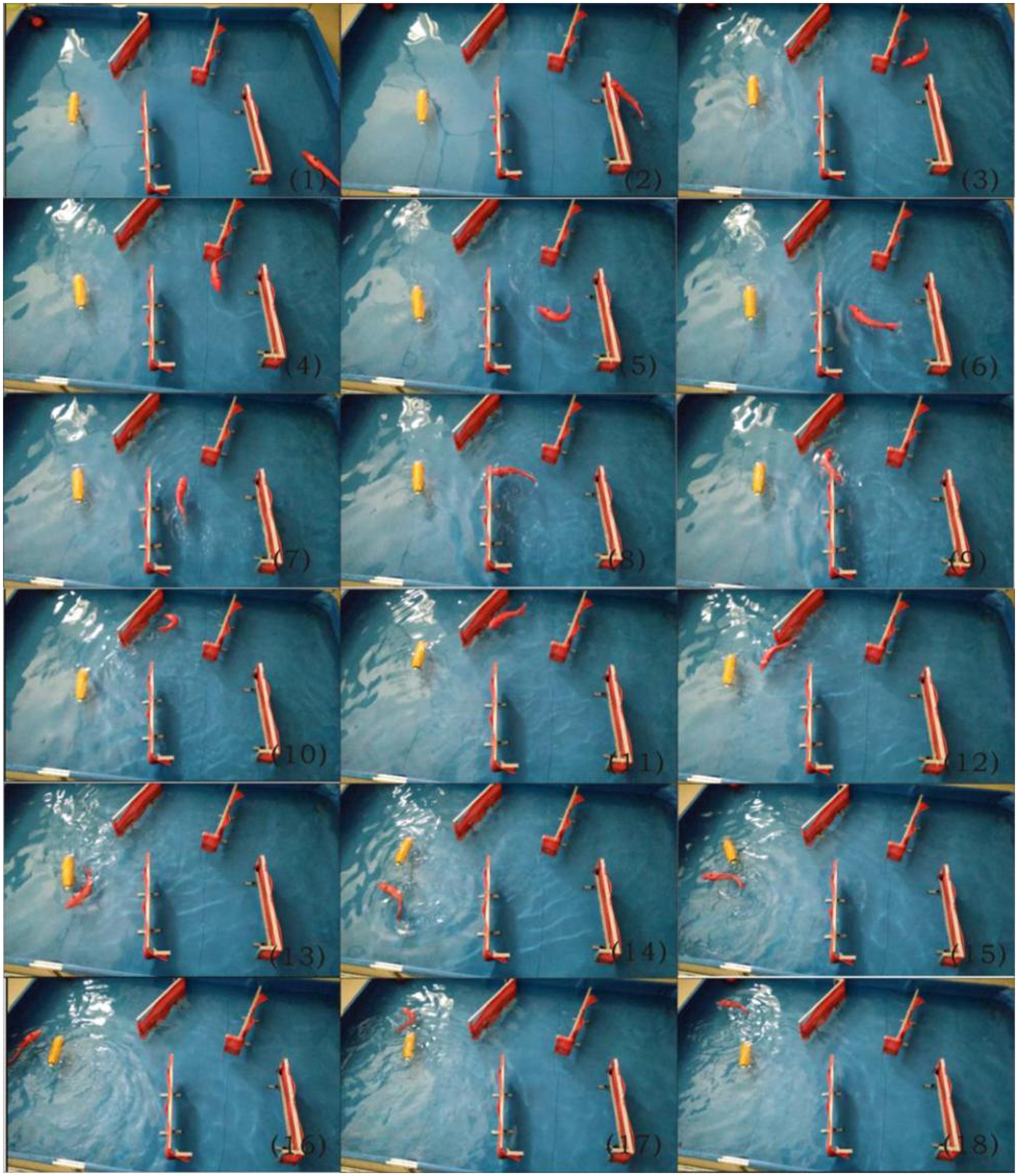
Figure 17. Obstacle avoidance and navigation process for robotic fish.
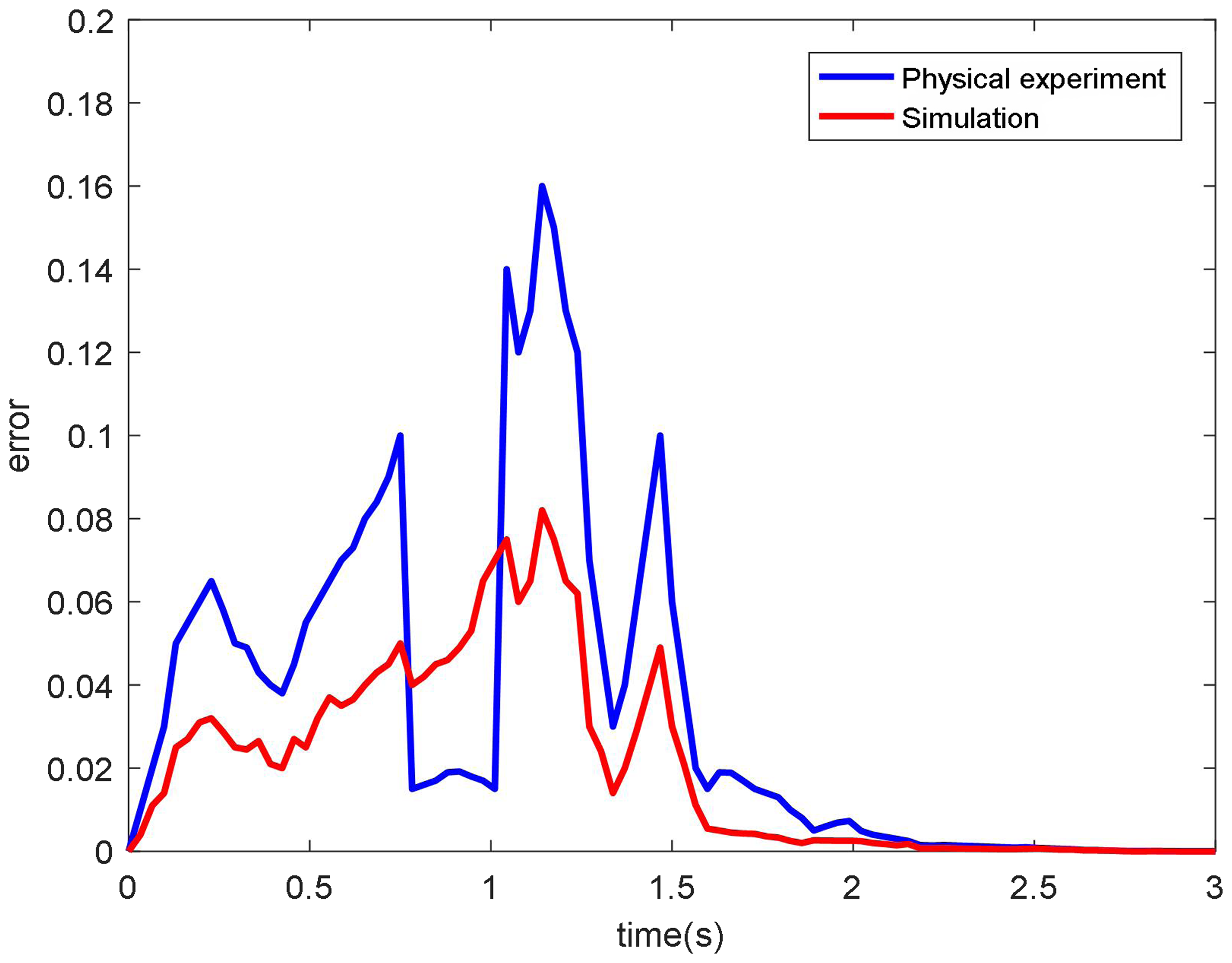
Figure 18. Comparison of error between simulation and physical experiment.
4.3. Physical experiment
A simple biomimetic robotic fish (also known as a mechanical fish, artificial fish, or fish-like robot) is used in the physical experiments. As shown in Fig. 14(a), the robot is a lightweight mobile robot, which is suitable for navigation experiments in underwater environments. Robots perceive the environment through external cameras and the camera coverage must cover the entire site. Therefore, two cameras located in the center of the navigation environment are set up. The cameras are Mercury MER-040-60UC models, as shown in Fig. 14(b). Visual positioning can be accomplished by calculating the coordinate system established on the site. The position of the bionic fish is tracked in real time.
The kinematic model [Reference Huang, Ruan, Yu, Fan, Li and Cai30] of the robotic fish is approximated by a polynomial and sinusoidal synthesis, as shown in formula (27).
 \begin{equation} {\boldsymbol{{f}}}_{{\boldsymbol{{B}}}}\left({\boldsymbol{{x}}},{\boldsymbol{{t}}}\right)=\left({\boldsymbol{{c}}}_{1}{\boldsymbol{{x}}}+{\boldsymbol{{c}}}_{2}{\boldsymbol{{x}}}^{2}\right)\sin \left(\omega {\boldsymbol{{t}}}+{\boldsymbol{{kx}}}\right) \end{equation}
where  ${\boldsymbol{{f}}}_{{\boldsymbol{{B}}}}({\boldsymbol{{x}}},{\boldsymbol{{t}}})$ is the lateral displacement of fish body, ${\boldsymbol{{c}}}_{1}$ is the primary coefficient of fish wave amplitude envelope. ${\boldsymbol{{c}}}_{2}$ is the quadratic coefficient of fish wave amplitude envelope, ${\boldsymbol{{k}}}$ is the wave number of fish wave ( ${\boldsymbol{{k}}}=2\pi /\lambda, \lambda$ is the wavelength of fish body wave), $\omega$ is the wave frequency of fish body ( $\omega =2\pi {\boldsymbol{{f}}}=2\pi /{\boldsymbol{{T}}}$).
The robot experiment takes place in a 3 m × 2 m × 0.35 m cuboid fish pond environment. Considering the size of the fish and the experimental environment, four static obstacles and one dynamic obstacle are set up, which make the environment more complex. The bionic fish starts cruising from the lower right corner of the space and the destination is set at the upper left side of the initial position. The top view of the experimental environment is shown in Fig. 15. The schematic diagram of the experimental environment is shown in Fig. 16. After the bionic fish starts to move, it traverses obstacles from the starting point of the environment to its destination. If the robot fish touches a wall, touches obstacles, or arrives at its destination, the experiment ends.
A video recording of the obstacle avoidance navigation process of the robot is made. Figure 17 shows some screenshots of a successful experiment.
When the robot deviates from the target point, there is navigation error. The degree and number of robots deviating from the target point are the magnitude of navigation error. We compare the navigation errors between the simulation experiment and the physical experiment as shown in Fig. 18. As shown in Fig. 18, there is a deviation between physical experiments and simulation experiments, and the simulation results are closer to the expected navigation in both the navigation accuracy and the convergence velocity. The main reason is that the robotic fish is seen as a particle in simulation experiment; however, the size of the robot fish cannot be ignored in physics experiments. However, simulation results provide many valuable references for physics experiments, such as learning methods and learning directions.
5. Conclusion
According to the Skinner OC mechanism, a hierarchical cognitive model is constructed to improve the self-learning and self-adaptive ability of mobile robots in unknown and complex environments. The cognitive model adopts the idea of dividing and conquering; it divides the navigation tasks of mobile robots in complex environments into sub-tasks at different levels and solves each sub-task in a smaller state subspace to reduce the dimension of the state space. The cognitive learning algorithm imitates the thermodynamic process to design and realize an online search, in order to determine the best navigation strategy.
Based on the formation of the cognitive process, the autonomous path planning activities of mobile robots were studied. The experimental results show that: (1) The cognitive model designed can enable mobile robots to successfully avoid obstacles in the environment and reach their goals via a better path. It can automatically acquire knowledge and accumulate experience from the environment, just like animals. Through cognitive learning, we have gradually formed, developed, and perfected autonomous path planning skills. (2) In time-varying and complex dynamic environments, robots can still quickly acquire the optimal path. The adaptive ability of robots shows that the hierarchical structure can reduce the learning difficulty of mobile robots in unknown complex environments, accelerate the learning speed, and avoid dimension disasters. (3) In order to prove the accuracy and rapidity of the hierarchical cognitive model, we compared it with the single cognitive model. The experimental results show that in the same complex environment, the navigation success rate of hierarchical structure is 94%, which is 14% higher than that of single structure. The running time of the layered structure is 200 s, 850 s higher than that of the single structure. (4) To prove the effectiveness of the design model HCNM, we compared it with a similar HRLM. The experimental results show that, in the same complex environment, HCNM navigation path is clearer and better than HRLM in experimental effect and convergence time, and the convergence time is accelerated by 160 s.
The significance of this paper is mainly in two aspects. On one hand, based on the operating conditional reflection mechanism of humans and animals, the paper designs cognitive learning behaviors similar to humans and animals for robot, enabling them to achieve autonomous navigation. It has certain guiding significance for artificial intelligence, robot technology, and cognitive science. On the other hand, compared with the operation-conditioned reflex learning model, the hierarchical cognitive model designed in this paper divides the navigation task of the mobile robot in the complex environment into different levels of sub-tasks through the hierarchical structure, which reduces the learning difficulty of the robot in the unknown environment and accelerates the learning speed of the robot. However, this method also has some limitations. After adding dynamic obstacles, the method needs four rounds of learning to converge, and the convergence speed is reduced, but the reduction is not obvious. In addition, for the selection of new paths, the hierarchical cognitive model needs to constantly try and make mistakes to find the best path. After the robot navigation method based on deep learning trains enough samples, the trained model can complete the navigation task of the new path without retraining. In the follow-up work, the application of deep learning methods in mobile robot navigation will be the next focus of the author.
Author contributions
Jianxian Cai and Fenfen Yan conceived and designed the study. Jianxian Cai and Yan Shi conducted the simulation experiments. Mengying Zhang and Lili Guo conducted the physical experiments. Jianxian Cai wrote the article.
Financial support
This work was supported by the Fundamental Research Funds for the Central Universities (J.X. and F.Y., grant numbers ZY20180112), Research and practice project of higher education reform in Hebei Province from 2019 to 2020 (J.X., grant numbers 2019GJJG471), Scientific Research Plan Projects for The National Key Research and Development Program of China (J.X., grant numbers 2018YFC1503801), the Scientific Research Project Item of Hebei Province Education Department (J.X., grant numbers QN2018317), The second batch of new engineering research and practice projects of the Ministry of Education (J.X., grant numbers E-SXWLHXLX20202607), 2020 education research and teaching reform project of College of disaster prevention technology (J.X., grant numbers JY2020A12).
Conflicts of interest
The authors declare none.


 Open access