


1. Introduction
Robots typically have actuators with a continuous range of actuation. From here, in this article, these robots are referred to as “continuous robots,” and their actuators will be called continuous actuators. What is expected of these robots is to track a trajectory with high precision. This involves the use of complex controller devices and programs that increase costs.
In some applications, such as picking and placing objects, the path of motion does not require high precision, but the points at the beginning and end of the path are important. Some investigators [Reference Pieper1, Reference Chirikjian2] have proposed that discrete actuators be used instead of continuous ones. Discrete actuators are actuators whose actuation values are limited to several values. For example, a binary prismatic actuator has only two stable states, fully retracted (0) and fully extended (1). Discrete actuators do not need feedback to be controlled. For example, for control of a binary pneumatic cylinder, it is only necessary to determine the direction of flow of compressed air correctly and give sufficient time to achieve a fully extended or fully retracted state. In this case, the piston moves so far to reach the end of its stroke. Simplicity in control, low controller equipment prices, high precision, and repeatability are all advantages of discrete actuators due to the lack of feedback.
When all the actuators of a robot are discrete, it is referred to as a discrete robot. The workspace of a discrete robot is formed from a finite set of discrete points, so one cannot expect a discrete robot to track a path with a high precision. For tracking a path by a discrete robot, it is necessary to select a few points among all points of the workspace so that they approximate the path in the best way. And then the robot moves from one point to another. Otherwise, the path that the robot tracks between two configurations is uncontrollable. Therefore, the number of workspace points must be greater so that access to the points and tracking of the path can be done more accurately. To do this, it is necessary to increase the number of actuation states of the actuators, or, more efficiently, the number of actuators.
Today researchers use discrete actuators in a variety of fields and devices such as grippers [Reference Chi, Tang, Liu and Yin3–Reference Tang, Chi, Sun, Huang, Maghsoudi, Spence, Zhao, Su and Yin9], switches [Reference Masana, Khazaaleh, Alhussein, Crespo and Daqaq10], medical imaging devices [Reference Miron, Girard, Plante and Lepage11–Reference Tappe, Boyraz, Korz and Ortmaier13], exoskeleton rehabilitation robots [Reference Cappello, Xiloyannis, Dinh, Pirrera, Mattioni and Masia14, Reference Dragone, Randazzini, Capace, Nesci, Cosentino, Amato, De Momi, Colao, Masia and Merola15], solar centralizing mirrors [Reference Lee, Bilton and Dubowsky16, Reference Rudolph, Nurnberger, Alqadah and Bobak17], millirobots [Reference Ze, Wu, Dai, Leanza, Ikeda, Yang, Iaccarino and Zhao18], microrobots [Reference Mohand-Ousaid, Bouhadda, Bourbon, Moal, Haddab and Lutz19–Reference Zhou and Xie21], and soft robots [Reference Patel, Huang, Luo, Mrunmayi Mungekar, Yao and Majidi22–Reference Son, Park, Na and Yoon25]. Some investigators use discrete actuators in hyper-redundant manipulators [Reference Chirikjian2, Reference Ebert-Uphoff26–Reference Kim, Jang and Nam29]. A hyper-redundant manipulator is typically made by cascading parallel mechanisms on top of each other as modules. For example, a VGTFootnote 1 module is illustrated in Fig. 1-a. Each module of VGT is a planar close chain mechanism consisting of three binary prismatic actuators (AC, AD, and BC links in Fig. 1-a) and two constant-length links (AB and CD links in Fig. 1-a). These links are passively joined in A, B, C, and D. The VGT module can be actuated into Ncon = 23 = 8 different states (configurations) by combining the actuation states of its actuators, as shown in Fig. 1-b. A VGT manipulator can be made by cascading VGT modules on top of each other.
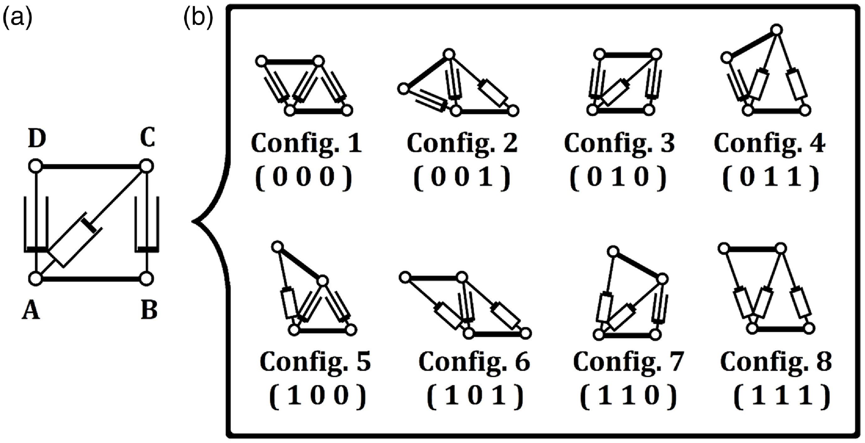
Figure 1. a) A VGT module. b) Configurations of a VGT module.
A four-module VGT manipulator (Nmod = 4) is shown in Fig. 2. The configuration number of the first module (the module that is connected to the base) is 4 (c1 = 4). The configuration numbers of the second, third, and last modules are 8, 3, and 6, respectively (c2 = 8, c3 = 3, c4 = 6). These numbers correspond to what is shown in Fig. 1-b. Based on what has been discussed earlier, a four-module VGT manipulator can have NconNmod = 84 = 4096 different configurations. Each configuration places the manipulator’s end-frame in a specific location. So, the workspace of this manipulator will include the same number of frames as illustrated in Fig. 3.

Figure 2. A 4-module VGT manipulator in configuration 4836 ( $\mathbb{C}=$
[c1 c2 c3 c4] = [4 8 3 6] ).
$\mathbb{C}=$
[c1 c2 c3 c4] = [4 8 3 6] ).
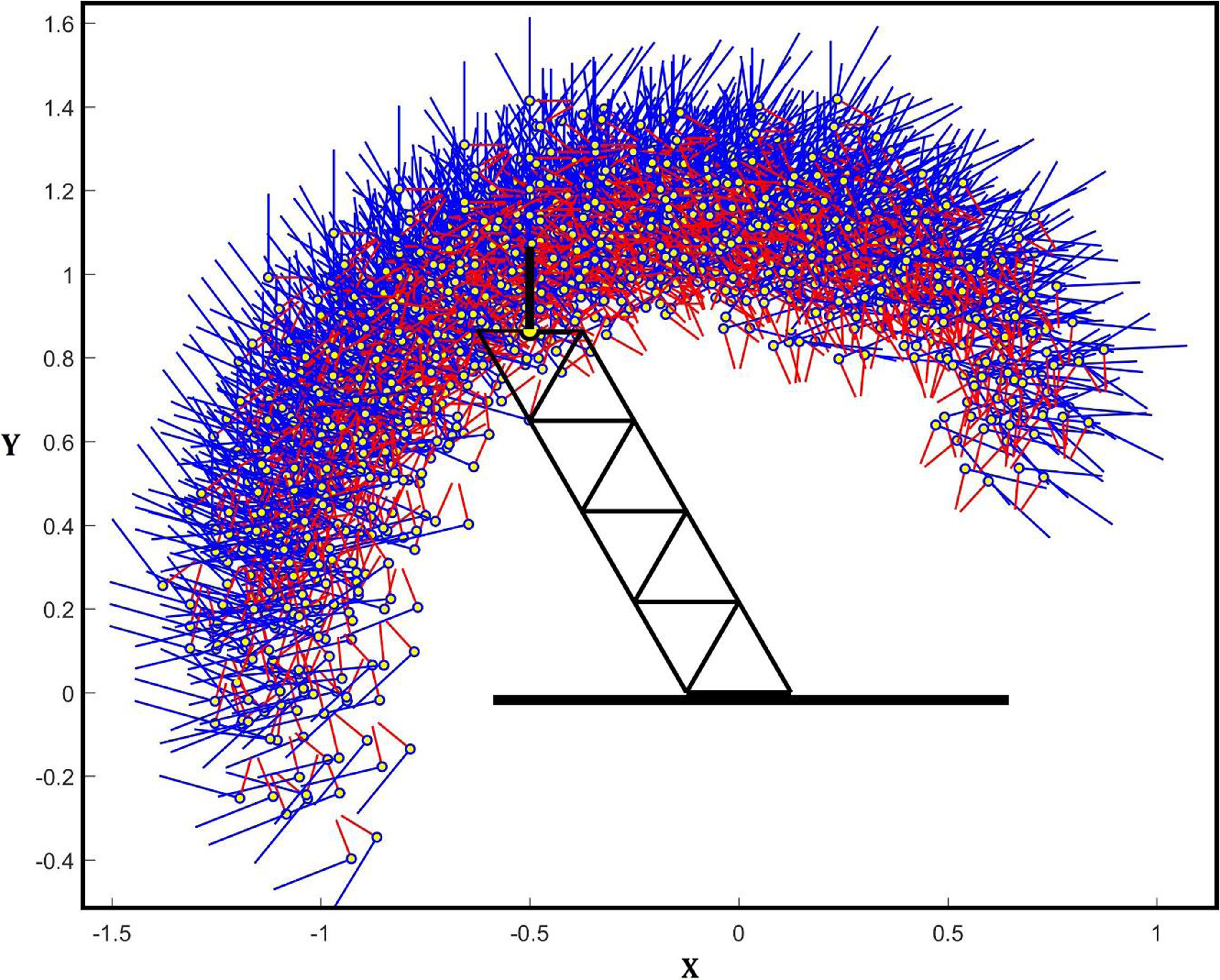
Figure 3. Workspace of a 4-module VGT manipulator containing 4096 discrete frames.
The hyper-redundant manipulators have the benefits of parallel robots, such as a high payload and high precision, combined with the benefits of serial robots, such as a large workspace and the ability to avoid obstacles. The use of discrete actuators instead of continuous ones eliminates the complex control problem of the hyper-redundant manipulators. From now on, this type of manipulator will be called “discretely actuated hyper-redundant manipulators (DAHRMs),” or in short, the “discrete manipulators.” In spite of the valuable capabilities described for discrete manipulators, they are practically underutilized. This may have been due to a lack of research. As for the inverse kinematics (IK) of these types of manipulators, as discussed below, there were deficiencies in existing publications, which was an incentive to present this article.
The IK problem is to determine the actuation amount of all the manipulator actuators so that the manipulator end-frame reaches a predetermined frame in space called the target-frame. As discussed later, in the case of DAHRMs, there are only a few choices for the actuation amount of each actuator. Therefore, the number of possible configurations for each module will be limited. As a result, the IK problem of DAHRMs becomes the choice of the best configuration from among all possible configurations, which minimizes the distance. In other words, the mentioned problem will be a combinatorial optimization problem, and it needs a different solution than what is proposed for continuous problems. The distance of the manipulator’s end-frame from the target-frame is considered the error of the answer to the IK problem. Here, the distance between two frames involves two concepts: location and direction.
Solving the forward kinematics problem of DAHRMs can be done without any problems. If the forward kinematic solution of each module is known, the transformation matrix of the manipulator can be calculated simply by multiplying the transformation matrix of the modules in sequence. But there are some problems with the methods presented in the field of IK. First, the usual methods used for continuous manipulators are not suitable for discrete manipulators because these methods do not necessarily lead to discrete values of actuation, and if the discrete values close to the values of the result are chosen instead, large errorsFootnote 2 are created. For example, Chirikijian and Lees [Reference Chirikjian and Lees30] approximated the overall shape of the manipulator to a spatial curve. And then they tried to close the end-frame to the target-frame by grasping the manipulator on this curve. But because the actuators are discrete, the modules have a limited number of configurations and could not sit well on the curve. The deviation of the modules from this curve, especially in the case of close-to-base modules, caused large errors in reaching the manipulator’s end-frame to the target-frame.
Secondly, the brute-force search method is not suitable. In this method, all configurations of the manipulator should be considered in the search space. The manipulator’s end-frame location should be calculated for all configurations of the manipulator (forward kinematics). These items are done off-line, and then the information is saved in the computer’s memory. After that, for solving an IK problem, it is sufficient to search among the saved information. This method is not feasible for the manipulators that have too many modules because the number of configurations grows exponentially with the increasing number of modules, and as a result, the CPU time and the required memory size grow exponentially too. In other words, the mentioned problem is an NP-hard problem, so brute-force searching is not feasible for it.
Ebert-Uphoff and Chirikjian [Reference Ebert-uphoff and Chirikjian31, Reference Ebert-Uphoff and Chirikjian32] used the concept of workspace density to solve the IK. When the workspace density of one point is higher than another, the manipulator has a better chance of reaching it. Their proposed method was a single-module searching algorithm. Here, the term “search” refers to the process of selecting the appropriate configuration among all possible configurations. And the term “single-module searching” refers to a searching process in which the searching space includes the configurations of a single module. Simply put, in a single-module searching process, the configuration of the manipulator was determined module by module. There are three types of modules in each step of this process:
-
1. Decided module: The module that has been configured in the previous steps.
-
2. Pending module: The module that is currently being configured.
-
3. Undecided module: The module that has not been configured.
In the first step, the pending module is the base module (the first module of the manipulator), and the rest of the modules are undecided. In the second step, the base module is a decided module, the second module is a pending module, and the other modules are undecided ones.
The searching process will continue until the last step, in which the pending module is the end module of the manipulator and the rest of the modules are decided modules. In the method discussed above, there is a concept called a “sub-workspace.” The sub-workspace is a subset of the manipulator workspace. To produce the sub-workspace, it is only required to freeze the pending and decided ones and allow only the undecided modules to move. At each step of the searching process, the criterion for selecting the pending module configuration is the greater than the target point density in the related sub-workplace. The problem with this method is the large amount of computation needed to calculate the sub-workspace density, especially in three-dimensional cases.
Suthakorn and Chirikjian [Reference Suthakorn and Chirikjian33] proposed another single-module searching method to solve this problem. Their searching algorithm was simpler and faster. They used the concept of sub-workspace mean-frame instead of sub-workspace density. The mean-frame of a sub-workspace was something like the mass center for a set of discrete masses. They provided an effective, simple, and fast way to calculate this frame and assumed that it had the highest density and that the density of each frame decreased by increasing its distance from the mean-frame. Therefore, their criterion for selecting the configuration of the pending module was to minimize the distance between the mean-frame of the corresponding sub-workspace and the target-frame. This method was very desirable in terms of CPU time and memory required, but its error was large.
Some investigators [Reference Sujan, Lichter and Dubowsky28, Reference dos Santos, Felipe and Sujan34] utilized genetic algorithms (GAs) to solve the IK problem of DAHRMs. In their method, the population size and the number of generations should be increased in order to obtain an acceptable precision, and with this, the CPU time will increase improperly. Kim et al. [Reference Kim, Jang and Nam29] proposed a continuous variable optimization method to solve the IK problem. They use a special cost function in order to lead the answers to the discrete values. This method was desirable in terms of CPU time and memory required, but the closeness of the results to discrete values was a challenging issue and depended on the subtle definition of the cost function.
Other meta-heuristic search methods, such as simulated annealing (SA) and particle swarm optimization (PSO), can also be used to solve the IK problem of DAHRMs. But as presented in the numerical results section, their results are weaker than the method presented in this article. In meta-heuristic search methods, two issues are important: exploration and exploitation. Exploration refers to the ability of the search to explore new and diverse regions of the solution space, while exploitation refers to the ability of the search to exploit the best solutions found so far and improve them locally. The exploration is done well, but the exploitation is not done well due to the lack of a suitable method to define neighbors in a controllable neighborhood radius. It causes a waste of time and inaccuracy. Anyway, solving this problem can lead to effective methods to solve the IK problem of DAHRMs. This issue can be investigated by researchers in the future.
Motahari et al. [Reference Motahari, Zohoor and Korayem35–Reference Motahari, Zohoor and Korayem38] proposed two new ideas in their search method: 1) Two-by-two searching or two-module searching, which means that two modules were configured in each step of the searching instead of one. These two were named “pending pair modules.” These two did not need to be adjacent. 2) Iteration, which means that when all modules are configured, repeating the search steps in a new order can improve the results and reduce errors. Their method did not necessarily find the exact solution, but it resulted in less error than the previous methods, and at the same time, it had a satisfactory CPU time. But the question that arises here is whether increasing the number of pending modules will improve the results. In other words, why not do three- or more-module searching instead of two-module searching? In this article, a generalized algorithm called “multi-module search (M-MS)” is presented to solve the IK problem of DAHRMs. Also, the effect of increasing the number of pending modules on CPU time and errors will be investigated.
In the M-MS method, the manipulator is initially configured randomly. Then, in each step, a certain number of modules (Npen) are randomly selected from all the modules of the manipulator as the pending modules. The search space in each step will contain all possible combinations of the configuration of the pending modules, and the best of them will finally be selected as the new configuration of these modules. This step is repeated by selecting the other pending modules randomly to reduce the error. The novelty of this method is the use of several modules instead of two in each step of the search. With this, a generalized method with the desired number of pending modules is presented.
The remainder of the article is organized as follows: in Section 2, the problem is stated clearly; after that, in Section 3, the proposed algorithm for solving the problem is described. Next, in Section 4, numerical results are presented. Finally, the conclusions are presented in Section 5.
2. Statement of the problem
Consider a prescribed frame as the target-frame (Ftar) and the end-frame of the manipulator (Fend). The end-frame location and orientation are determined if and only if the configuration of the manipulator ( $\mathbb{C}$
) is determined. To do this, all modules should be configured (
$\mathbb{C}$
) is determined. To do this, all modules should be configured ( $\mathbb{C}$
= [c1 c2 … cNmod]). The IK problem of a DAHRM that contains Nmod modules, each with Ncon configurations, can be described as a discrete variable optimization problem as below:
$\mathbb{C}$
= [c1 c2 … cNmod]). The IK problem of a DAHRM that contains Nmod modules, each with Ncon configurations, can be described as a discrete variable optimization problem as below:
 \begin{equation}\underset{\mathbb{C}}{\textbf{Minimize}} \left(\textbf{Error}(\mathbb{C})=\textbf{ Distance}\left(\textbf{F}_{\textbf{end}}(\mathbb{C}), \textbf{F}_{\textbf{tar}}\right)\right)\end{equation}
where $\mathbb{C}$
= [c1 c2 … cNmod]
$\mathbb{C}$
= [c1 c2 … cNmod]
subjected to
ci $\epsilon$
{1, 2, …, Ncon} for i = 1, 2, …, Nmod
$\epsilon$
{1, 2, …, Ncon} for i = 1, 2, …, Nmod
In the above expression, Error, which equals the distance between Fend and Ftar, is considered an objective function that is a function of the manipulator configuration ( $\mathbb{C}$
).
$\mathbb{C}$
). $\mathbb{C}$
can be selected from a set of all possible configurations of the manipulator. In other words, the modules should be configured so that the end-frame is as close to the target-frame as possible.
$\mathbb{C}$
can be selected from a set of all possible configurations of the manipulator. In other words, the modules should be configured so that the end-frame is as close to the target-frame as possible.
Figure 4 is presented for more familiarity with the IK problem of DAHRMs. Figure 4-a shows a VGT manipulator consisting of two modules (Nmod = 2) that must reach the target-frame (Ftar) represented by the dashed-line. Each module has a binary prismatic actuator, so it has two configurations (Ncon = 2), as shown in Fig. 4-b. By combining the possible configurations of the modules, the manipulator will have NconNmod = 22 = 4 configurations, as shown in Fig. 4-c. As can be seen in Fig. 4-c, among all configurations, the end-frame (Fend) of configuration No. 21 ( $\mathbb{C}$
= [2 1]) is closer to the target-frame (Ftar). Therefore, this configuration will be the best answer to the problem.
$\mathbb{C}$
= [2 1]) is closer to the target-frame (Ftar). Therefore, this configuration will be the best answer to the problem.

Figure 4. An example of the IK problem of DAHRMs.
The distance of the manipulator’s end-frame from the target-frame is considered the error of the answer to the IK problem. Here, the distance is not just the distance between the two origins; the difference in the direction of the two frames should also be considered. Formulas for calculating the distance between two frames are presented in the appendix. According to the definition of the error, even the best answer may have some errors, as can be seen in Fig. 4-c. But all the sample problems solved in the numerical results section are chosen to have an exact solution (zero error) to make sure the error in the answer is due to the solution method.
As mentioned in the introduction section, ordinary methods used for solving the IK problem of continuous manipulators are not usable for DAHRMs because they lead to big errors. So, solving this problem requires a special method. On the other hand, due to the large number of the manipulator configurations, it is not feasible to use brute-force searching. Among the methods presented in the articles, the two-by-two searching method has the best results in terms of error and CPU time. Two ideas have been used in this method: two-module searching and iteration. In the two-by-two searching method, there are two pending modules in each step of the solution, which are chosen randomly among all manipulator modules. Iterating this process reduces the error. The question that arises here is: Does increasing the number of pending modules lead to better results? To answer this question, a comprehensive method with an arbitrary number of pending modules is designed based on the two-by-two searching method, which is named “multi-module search (M-MS).” Step-by-step explanation of this method is as follows:
-
Step 1: The manipulator is configured arbitrarily.
-
Step 2: A certain number of modules (Npen) are arbitrarily selected from among all manipulator modules. These modules are known as pending modules.Footnote 3
-
Step 3: In this step, a new configuration for the pending modules is selected to reduce the error. The search space for this selection includes all the configuration combinations of the pending modules. The selection criterion is the error value. For example, if the number of pending modules is two (Npen = 2), and each module has eight configurations (Ncon = 8), the search space in this step contains NconNpen = 82 = 64 configurations. By changing the configuration of the pending modules, the configuration of the manipulator will also change. This new configuration, called the candid configuration, has a different error. All possible configuration combinations for the pending modules should be tested, and the related error should be calculated. Then, from among the candidate configurations, the configuration that has the least error is considered the new configuration of the manipulator.Footnote 4
-
Step 4: If the error value is greater than a predetermined threshold, then go back to step 2 and repeat the steps above. Otherwise, terminate the execution of the steps.
Step 3 is illustrated in Fig. 5 for a ten-module VGT manipulator using two randomly selected pending modules. In this figure (as in Fig. 4), each module contains a binary prismatic actuator. Therefore, in each iteration, there will be NconNpen = 22 = 4 candidate configurations.
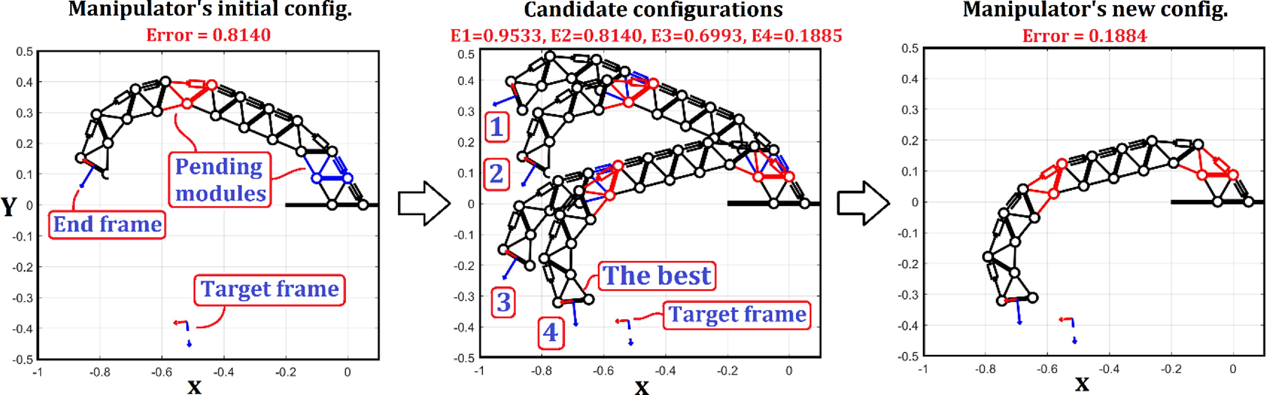
Figure 5. The process of selecting a new configuration for a ten-module VGT manipulator using two randomly selected pending modules. This process can be repeated for the new configuration to reduce the error.
In the second step, modules are not required to be selected in a particular order or adjacently. Numerical results show that if the initial configuration in Step 1 is chosen based on the “middle actuationFootnote 5” (as is done in the two-by-two searching method), it will lead to slightly better results than the random configuration. But the “middle configuration” is an unrealistic configuration, and all these configurations must be replaced with real configurations in the iteration steps. As a result, the algorithm will be a little more complicated. For this reason, this improvement is omitted here, and a random configuration is used in Step 1.
The search space of the proposed method, which contains all the candidate configurations, is far smaller than that of the brute-force searching method. The search space in the brute-force searching method includes NconNmod configurations. Now, if the number of iterations is Nitr, then the search space of the M-MS method will contain Nitr × NconNpen configurations. Therefore, the search space of the brute-force approach would grow exponentially as the number of modules increased, but in the multi-module method, the search space is not dependent on the number of manipulator modules (Nmod).
The number of cost evaluations in the M-MS method will be the same (Nitr × NconNpen). The CPU time will be proportional to this value. Accordingly, the time complexity of brute-force, two-by-two search and M-MS methods with respect to the size of input parameters is presented in Table I using big O. As can be seen in Table I, the M-MS method has exponential time with respect to the size of pending modules. This means that with the increase in Npen, the CPU time grows exponentially in the M-MS method. Npen in the two-by-two search method equals two and is not changed. Nmod in brute force has an exponential effect, but in the two-by-two and M-MS methods, its effect is linear. Nmod in these two methods affects the time of evaluating the cost function because the transformation matrix of the modules must be multiplied together to calculate the transformation matrix of the manipulator.
Table I. Time complexity of brute-force, two-by-two search, and M-MS methods with respect to the size of input parameters, using big O.
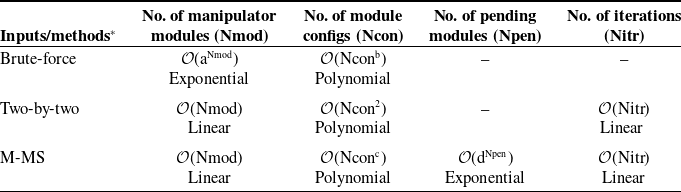
*a, b, c, and d are some constants: Ncon, Nmod, Npen, and Ncon, respectively.
To make the described method clearer, the related algorithm is presented below:
% M-MS algorithm:
Input( Nmod, Npen, Ncon )
-
% Nmod is the number of modules in the manipulator.
-
% Npen is the number of pending modules in each step of iteration.
-
% Ncon is the number of configurations of the modulesFootnote 6.
Input( { T1, T2, …, TNcon }, Ttar )
-
% Ti is the homogeneous transformation matrix of the module in its i’th configuration ( i = 1, 2, …, Ncon ).
-
% Ttar represents the transformation matrix of the target- frame.
Input( $\varepsilon$
)
$\varepsilon$
)
% $\varepsilon$
is a threshold for allowable error.
$\varepsilon$
is a threshold for allowable error.
For i = 1 : Nmod
ci = randi(Ncon) ;
-
% ci represents the chosen configuration of the i’th module in this step of the solution. At first, it is chosen randomly, but it may be changed later in the iteration steps.
-
% randi(n) is a function that returns a random integer on the interval 1 to n.
End
[A1, A2, …, ANmod ] = [ $\mathrm{T}_{{\mathrm{c}_{1}}}$
,
$\mathrm{T}_{{\mathrm{c}_{1}}}$
, $\mathrm{T}_{{\mathrm{c}_{2}}}$
, …,
$\mathrm{T}_{{\mathrm{c}_{2}}}$
, …, $\mathrm{T}_{{\mathrm{c}_{\text{Nmod}}}}$
] ;
$\mathrm{T}_{{\mathrm{c}_{\text{Nmod}}}}$
] ;
-
% Ai is the homogeneous transformation matrix of the i’th module of the manipulator.
A_man = A1 A2 … ANmod ;
-
% A_man is the transformation matrix of the manipulator, which represents the position and orientation of the end effector related to the base.
Error = distance( A_man, Ttar ) ;
-
% distance(A,B) is a function that calculates the distance between two frames A and B. The formula for this function is given in the appendix.
nitr = 0 ;
-
% nitr represents the number of iterations in this step of the solution.
While Error > $\varepsilon$
nitr = nitr + 1
[ m1, m2, …, mNpen ] = sort( randsample( Nmod, Npen ) ) ;
-
% mi is an integer between 1 and Nmod, which indicates which module of the manipulator is considered the i’th pending module.
-
% randsample(A,B) is a function that chooses B non-repetitive integers randomly on the interval 1 to A.
-
% sort(V) is a function that sorts the vector of numbers V.
For k1 = 1 : Ncon
For k2 = 1 : Ncon
⋮
For kNpen = 1 : Ncon ${\mathrm{c}_{\mathrm{m}}}_{1}$
= k1 ;
${\mathrm{c}_{\mathrm{m}}}_{1}$
= k1 ; ${\mathrm{c}_{\mathrm{m}}}_{2}$
= k2 ;
${\mathrm{c}_{\mathrm{m}}}_{2}$
= k2 ; $\vdots$ ${\mathrm{c}_{\mathrm{m}}}_{\text{Npen}}$
= kNpen ;
${\mathrm{c}_{\mathrm{m}}}_{\text{Npen}}$
= kNpen ;
[ A1, A2, …, ANmod ] = [ $\mathrm{T}_{{\mathrm{c}_{1}}}$
,
$\mathrm{T}_{{\mathrm{c}_{1}}}$
, $\mathrm{T}_{{\mathrm{c}_{2}}}$
, …,
$\mathrm{T}_{{\mathrm{c}_{2}}}$
, …, $\mathrm{T}_{{\mathrm{c}_{\text{Nmod}}}}$
] ;
$\mathrm{T}_{{\mathrm{c}_{\text{Nmod}}}}$
] ;
A_man = A1 A2 … ANmod ; $\mathrm{E}_{{\mathrm{k}_{1}}{\mathrm{k}_{2}}\cdots {\mathrm{k}_{\text{Npen}}}}$
= distance( A_man, Ttar ) ;
$\mathrm{E}_{{\mathrm{k}_{1}}{\mathrm{k}_{2}}\cdots {\mathrm{k}_{\text{Npen}}}}$
= distance( A_man, Ttar ) ;
-
% Ei j … k is the error related to the choice: the first pending module is in the i’th configuration, the second one is in the j’th configuration and so on until the last one, which is in the k’th configuration.
End
⋮
End
End
[ $\mathrm{c}_{{\mathrm{m}_{1}}}$
,
$\mathrm{c}_{{\mathrm{m}_{1}}}$
, $\mathrm{c}_{{\mathrm{m}_{2}}}$
, …,
$\mathrm{c}_{{\mathrm{m}_{2}}}$
, …, $\mathrm{c}_{{\mathrm{m}_{\text{Npen}}}}$
] = index( min { E11…1, E11…2, …,
$\mathrm{c}_{{\mathrm{m}_{\text{Npen}}}}$
] = index( min { E11…1, E11…2, …, $\mathrm{E}_{\text{Ncon Ncon}\ldots \text{Ncon}}$
} ) ;
$\mathrm{E}_{\text{Ncon Ncon}\ldots \text{Ncon}}$
} ) ;
-
% min { A, B, …, C } is a function that returns the minimum number in the set { A, B, …, C }.
-
% index(Aij…k) is a function that returns the index of Aij…k as a vector of integers [ i, j, …, k ].
Error = min { E11…1, E11…2, …, $\mathrm{E}_{\text{Ncon Ncon}\ldots \text{Ncon}}$
} ;
$\mathrm{E}_{\text{Ncon Ncon}\ldots \text{Ncon}}$
} ;
-
% Error is the distance related to the $\mathbb{C}=[\mathrm{c}_{1},\mathrm{c}_{2},\ldots, \mathrm{c}_{\text{Nmod}}]$
.
$\mathbb{C}=[\mathrm{c}_{1},\mathrm{c}_{2},\ldots, \mathrm{c}_{\text{Nmod}}]$
.

End
Display( c1, c2, …, cNmod ) ;
-
% The main output of the algorithm, which is the solution of the IK problem, is a set of integers, each of which is on the interval 1 to Ncon and represents the configuration of each module of the manipulator.
Nitr = nitr ;
-
% Nitr is the number of iterations occurred in the solution process.
Display(Nitr)
Display(Error)
-
% Here Error represents the error of the final solution.
Figure 6 illustrates the flowchart of the M-MS method.
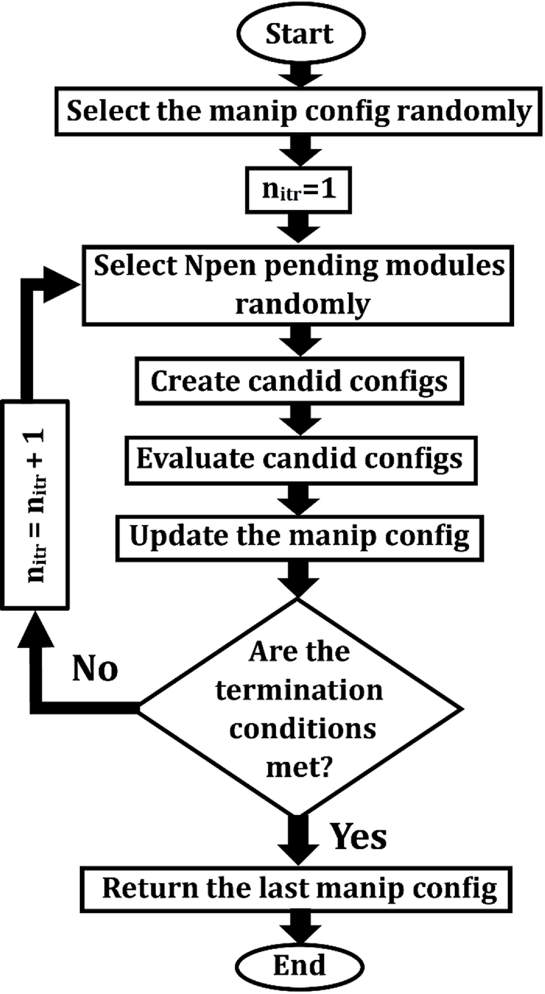
Figure 6. Flowchart of the M-MS method.
3. Numerical results
In this section, the method of calculating error is first described, then a 2D and a 3D case study are introduced, and finally, numerical results are presented in tables and diagrams and analyzed.
3.1. Definition of error
As discussed in Section 1, the workspace of a discrete manipulator is a finite set of discrete frames in space. If the target-frame is selected from among the frames in this set, the IK problem will have an exact solution; otherwise, even the best solution will not fit the target-frame. For the error to be real, all the problems discussed in this section will be of the first type, which is called “real problems.” For this purpose, the target-frame is derived by solving a forward kinematic problem with a random configuration. The error is defined as the distance between the target-frame and the manipulator end-frame, related to the configuration of the answer to the problem. The distance between the two frames is calculated using the definition given by Park [Reference Ebert-Uphoff26] and described in Appendix A. In order to compare the error of various problems correctly, these errors should be dimensionless. To do this, the distance mentioned is divided by the shortest length of the manipulator. The length of the manipulator is the distance between the origin of the base-frame and the origin of the end-frame of the manipulator.
3.2. Introducing the case studies
3.2.1. 2D case study
A 20-module manipulator with similar VGT modules is considered the 2D case study. This manipulator is called the ‘‘VGT manipulator.’’ A VGT module introduced earlier in Section 1 and illustrated in Fig. 1. The lengths of the constant links (AB and CD in Fig. 1) are 1/20. As mentioned earlier, all actuators in this module are binary. The discrete amounts of actuation (which are the length of the links, AD, AC, and BC) are 1/20 and 1.5/20. Thus, the minimum and maximum lengths of the manipulator are Lmin = 1 and Lmax = 1.5, respectively. Readers are referred to Kim et al. [Reference Kim, Jang and Nam29] for the forward kinematics of this module.
3.2.2. 3D case study
A 20-module manipulator with similar 3-RPS modules is considered the 3D case study. This manipulator is called, in short, the ‘‘3-RPS manipulator.’’ A 3-RPS module, as shown in Fig. 7, is a spatial parallel robot with three binary prismatic actuators in its three legs, A1B1, A2B2, and A3B3. The baseplate (A1A2A3) and the moving plate (B1B2B3) are equilateral triangles. A1, A2, and A3 are passive revolute joints with rotation axes parallel to their opposite sides in triangle A1A2A3. B1, B2, and B3 are passive spherical joints. The distances between the center and corners of the two triangles are a = b = 1/20. The discrete amounts of actuation, which are the length of the legs, are 1/20 and 1.5/20. So, the minimum and maximum lengths of the manipulator are Lmin = 1 and Lmax = 1.5, respectively. Readers are referred to Kim et al. [Reference Kim, Jang and Nam29] for the forward kinematics of this module.
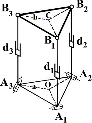
Figure 7. A 3-RPS module.
3.3. Numerical results
Figure 8a and b is presented to investigate the effect of the number of iterations (Nitr) on the error and the CPU time, respectively, for the 2D and 3D case studies. In both figures, the results for the 2-MS and 3-MS methodsFootnote 7 are presented. The presented results are the average results of 100 real random problems. Of course, these 100 problems are considered common among all cases so that their results can be compared. All the calculations in this article were done with MATLAB software and an Intel 1.66 GHz processor.
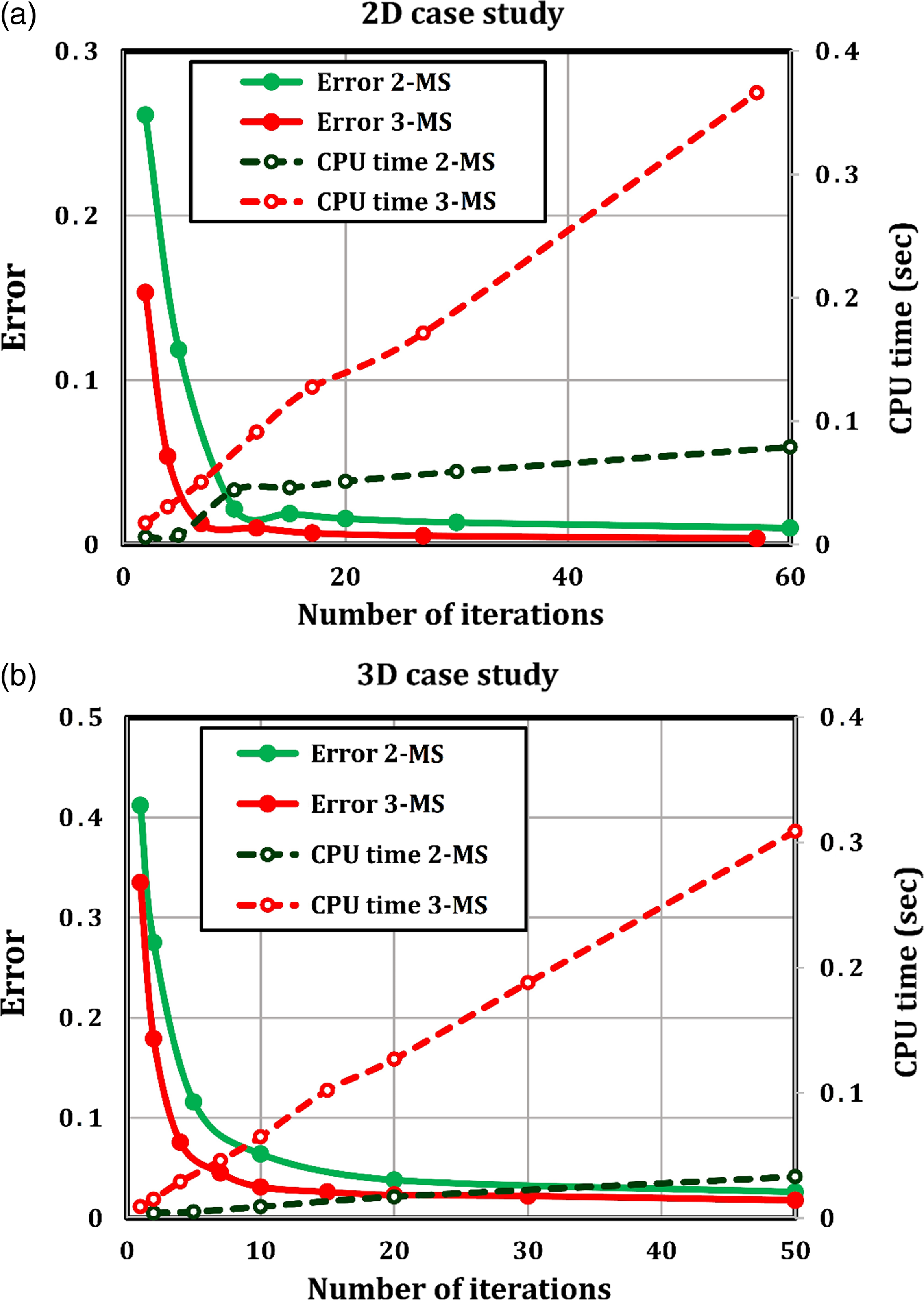
Figure 8. Examining the effect of the number of iterations on error and CPU time of the 2D case study (a) and the 3D case study (b) in two 2-MS and 3-MS methods.
According to these two figures, it is generally seen that the error decreases with the increase in Nitr, but the rate of this decrease decreases with the increase in Nitr until it remains constant after several iterations. On the other hand, the CPU time increases almost linearly with the increase in Nitr. The slope of this line is, as expected, higher in the 3-MS than in the 2-MS because, as mentioned in Section 3, the number of configurations examined in each step of the iteration in the three-module search is eight times that of the two-module search. In an equal Nitr, the error of the 3-MS is less than that of the 2-MS, but the CPU time is longer.
The numerical results presented in Fig. 8 showed that increasing the number of pending modules (Npen) reduces the error, but at the same time, the CPU time increases. Therefore, choosing Npen will be a challenge that should be considered.
Figure 9-a and b is presented for 2D and 3D case studies, respectively, to investigate the effect of increasing Npen on the efficiency of the solution method. For this purpose, the performance of 1-MS, 2-MS, 3-MS, and 4-MS methods has been compared. In each of the mentioned methods, the problem has been solved for various amounts of Nitr, and in each case, the CPU time and error have been evaluated. Then these points are connected by a curve in the CPU time error diagram. The presented results are the average results of 100 real random problems. Of course, these 100 problems are considered common among all cases so that their results can be compared.
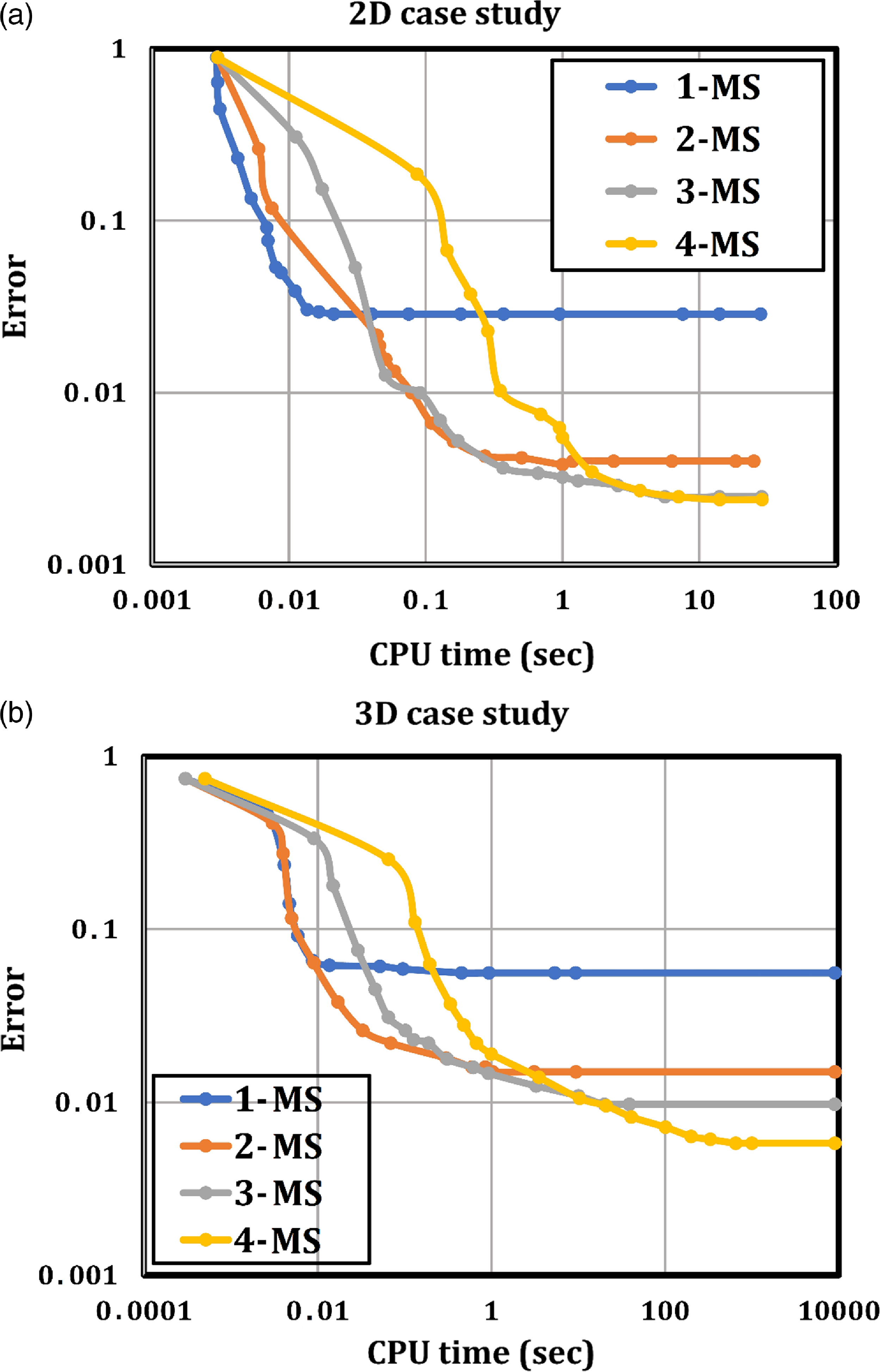
Figure 9. Comparison of the performance of 1-MS, 2-MS, 3-MS, and 4-MS methods in terms of error and CPU time for the 2D case study (a) and the 3D case study (b).
According to these two figures, in general, it is not possible to say which method is better than the others. Rather, in each time interval, the best method may be different. In short times (less than 0.01 s), the error increases with the increase of Npen, but in longer times, this advantage is gradually reversed, for example, in times of more than 10 s, in both figures, the lowest error belongs to 4-MS, followed by 3-MS, 2-MS, and 1-MS methods, respectively. Therefore, in general, it is not possible to decide on the amount of Npen, and the maximum acceptable CPU time for the problem should be determined. A CPU time below 1 s is usually considered acceptable for online problems. In this case, it can be seen in both figures that the 2-MS and 3-MS methods are superior to the 1-MS and 2-MS methods. In this case, the competition between the 2-MS and 3-MS methods is close, but the 3-MS is a little better. Note that both the horizontal and vertical axes are logarithmic.
Figure 10 is presented to validate the efficiency of the proposed algorithm. In this figure, the 2-MS and 3-MS methods are compared with nine meta-heuristic algorithms: the SA algorithm, GA, PSO, ant colony optimization (ACO), gray wolf optimizer (GWO), stochastic fractal search (SFS), whale optimization algorithm (WOA), Giza pyramid construction (GPC), and flying fox optimization (FFO) algorithm, all for the 2D case study (Fig. 10-a) and the 3D case study (Fig. 10-b).
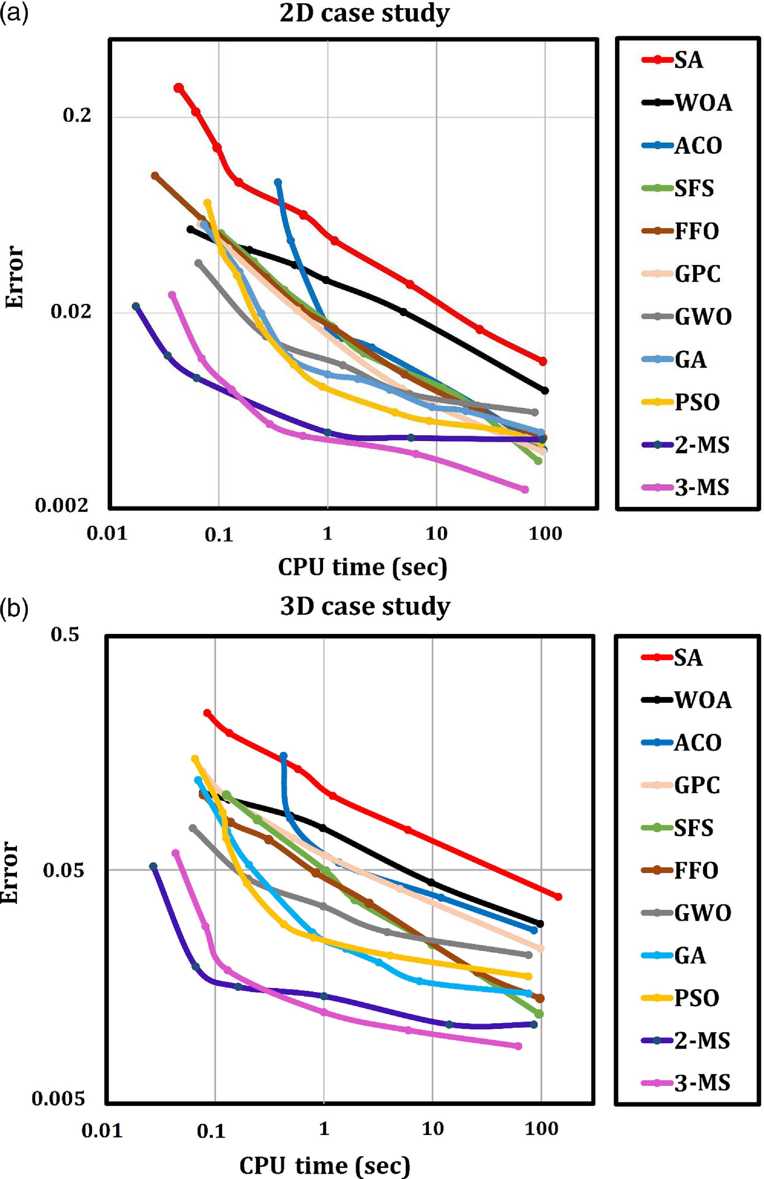
Figure 10. Comparing the performance of 2-MS and 3-MS methods with nine meta-heuristic search algorithms: SA, WOA, ACO, GPC, SFS, FFO, GWO, GA, and PSO, for the 2D case study (a) and the 3D case study (b).
In all methods, a common random problem has been solved one hundred times, and the average values of the results are presented. For the SA, GA, and PSO algorithms, the special functions for them, which are available in MATLAB, have been used. For the ACO, GWO, SFS, WOA, GPC, and FFO, the prepared codes in Refs [Reference Heris40–Reference Zervoudakis45] are used, respectively.
In the SA algorithm, for both 2D and 3D case studies, the initial temperature is 100 and the re-annealing interval is 100. By changing the maximum iteration value, different points of the corresponding curve are obtained in the figure. In GA, for both 2D and 3D case studies, the population size is 200, the elite count is 2, and the crossover fraction is 0.8. By changing the value of generation, different points of the corresponding curve are created in the figure. In PSO, for both 2D and 3D case studies, the value of particle swarm is 100, and different points of the curve are obtained from the change in the max-iterations value.
In ACO, for both 2D and 3D case studies, the number of iterations is 50, and different points of the curve are obtained from the change in the number of ants. In GWO, for both 2D and 3D case studies, the number of search agents is 50, and different points of the curve are obtained from the change in the max-iterations value. In SFS, for both 2D and 3D case studies, the number of start points (population size) is 10, the maximum number of diffusion (number of neighbors) is 10, and different points of the curve are obtained from the change in the maximum generation value.
In WOA, for both 2D and 3D case studies, the number of search agents (population size) is 100, and different points of the curve are obtained from the change in the maximum iterations value. In GPC, for both 2D and 3D case studies, maximum number of iterations (days of work) is 50, the value of substitution probability is 0.1, and different points of the curve are obtained from the change in the number of workers (population size). In FFO, for both 2D and 3D case studies, different points of the curve are obtained from the change in the maximum number of evaluating the cost function.Footnote 8 The remaining parameters are set to default values in all meta-heuristic algorithms mentioned above. Readers can find more information on the nine mentioned meta-heuristic algorithms in references [Reference Kirkpatrick, Gelatt and Vecchi46–Reference Zervoudakis and Tsafarakis54].
According to the figure, it can be said that in both 2D and 3D case studies, the 2-MS and 3-MS methods are superior to the nine meta-heuristic search methods. In the comparison between the two methods, 2-MS and 3-MS, as it was said about Fig. 9, it is not possible to comment in general, but it depends on the CPU time interval. In both 2D and 3D case studies, in CPU times less than 0.1 s, 2-MS is superior, but in CPU times close to 1 s and more, 3-MS performs better. It is not possible to form a general opinion about the nine meta-heuristic search algorithms, and the situation is different at different CPU time intervals. For example, for a CPU time of 1 s in the 2D case study, the following meta-heuristic algorithms work better in order: PSO, GA, GWO, GPC, ACO, SFS, FFO, WOA, and SA. In the 3D case study, the order is slightly different: PSO, GA, GWO, FFO, SFS, ACO, GPC, WOA, and SA. In both 2D and 3D case studies, it can be said that in the comparison between the nine meta-heuristic algorithms, algorithms PSO, GA, and GWO have the best performance and algorithms SA and WOA have the worst performance. Note that both the horizontal and vertical axes are logarithmic.
The proposed method and the nine presented meta-heuristic search algorithms are all nondeterministic search algorithms, which give different results from different runs. For this reason, in the previous diagrams, the problems were solved 100 times, and the average values of the results were presented.
An algorithm will be more robust if its answer changes less during different executions for the same input. To validate the robustness of the proposed method, a common random real problem has been solved one hundred times in both 2D and 3D case studies in 1 s, and the standard deviation of the errors of the 2-MS and 3-MS methods has been compared with the nine meta-heuristic algorithms in Fig. 11. Figure 11-a and b is related to the 2D and 3D case studies, respectively.
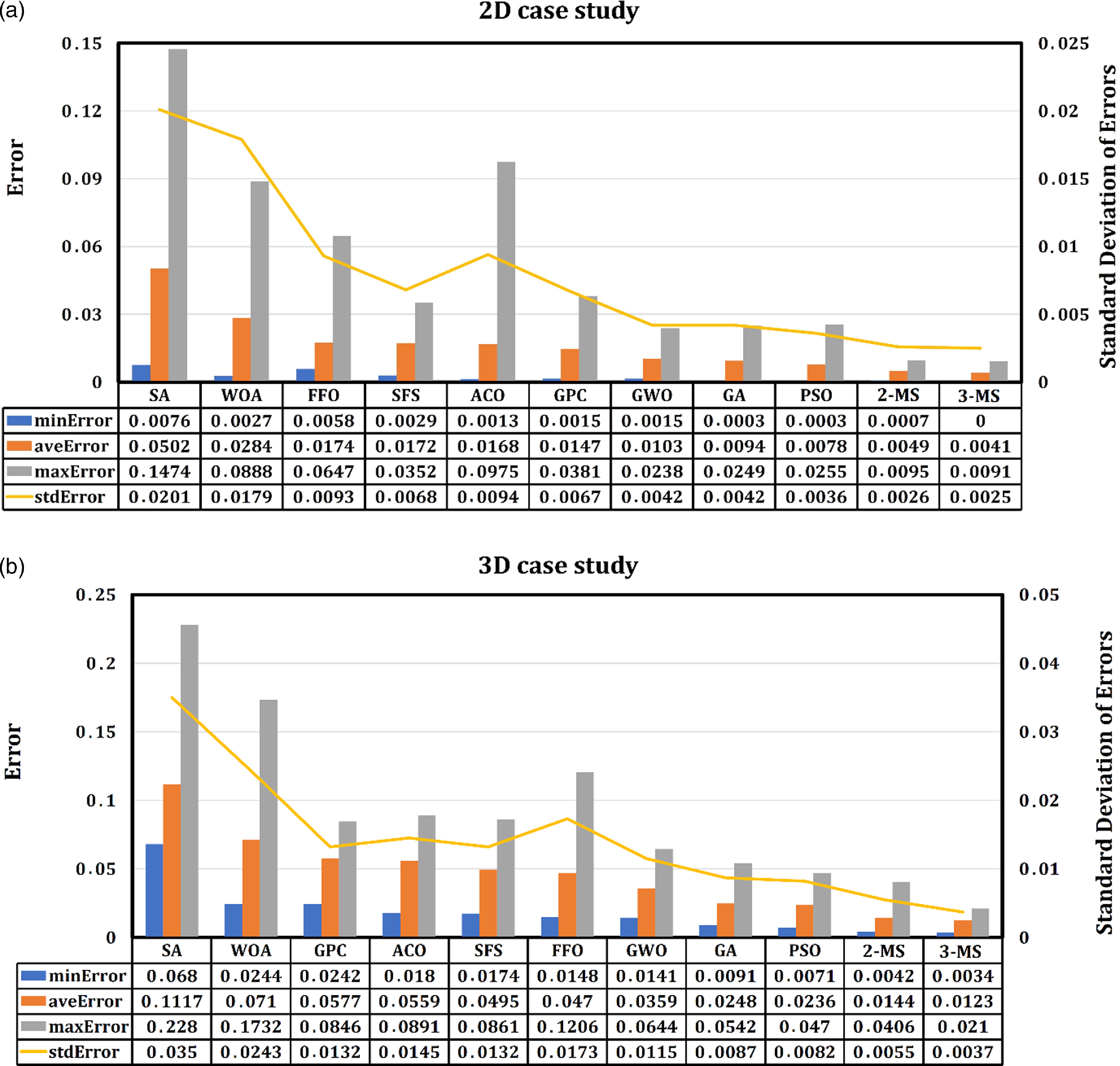
Figure 11. Comparison of the error of 2-MS and 3-MS methods with nine meta-heuristic search algorithms: SA, WOA, ACO, GPC, SFS, FFO, GWO, GA, and PSO, all in 1 s CPU time, for two case studies: 2D (a) and 3D (b).
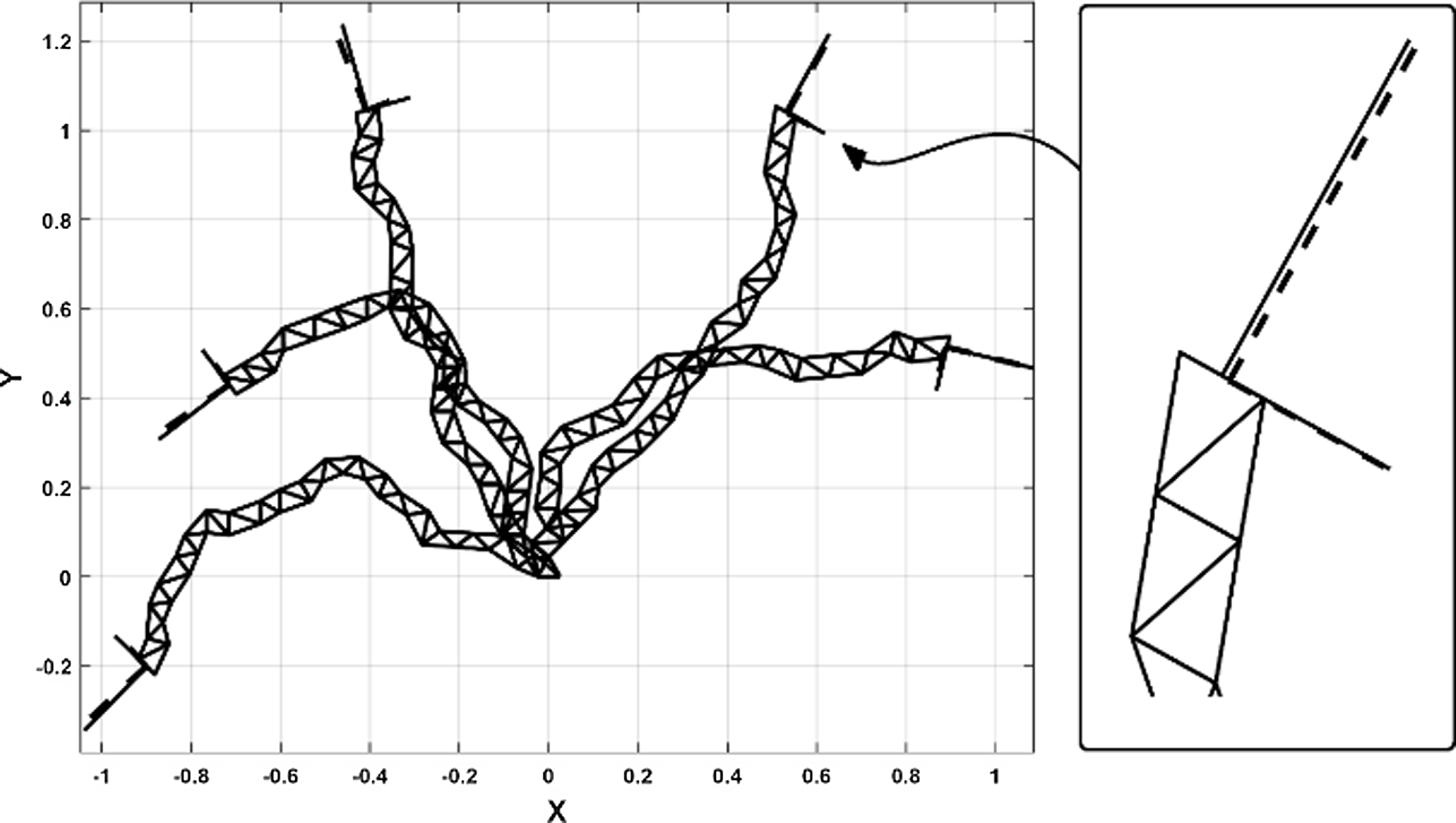
Figure 12. The solution configurations of five real random IK problems for the 2D case study, which were solved using the 3-MS method with 50 iterations. The end frames are represented by solid lines, while the target frames are represented by dashed lines.

Figure 13. The solution configurations of five real random IK problems for the 3D case study, which were solved using the 3-MS method with 50 iterations. The end frames are represented by solid lines, while the target frames are represented by dashed lines.
The minimum, average, maximum, and standard deviation (std) of the errors have been obtained for each method. The smaller the standard deviation of the error, the more robust the method will be. The standard deviation of the error is represented by an orange curve. Based on this, the order of robustness of the algorithms in the 2D case study, from more to less, is as follows: 3-MS, 2-MS, PSO, GA, GWO, GPC, SFS, FFO, ACO, WOA, and SA. The 3D case study follows the same order, but the ACO and FFO are swapped out. The order of the bar graphs is based on the average error. In both 2D and 3D case studies, methods 3-MS and 2-MS are more robust than the nine meta-heuristic algorithms. In the comparison between nine meta-heuristic algorithms in both 2D and 3D case studies, algorithms PSO, GA, and GWO are the most robust, and algorithms SA and WOA are the least robust (similar to the average error).
Figures 12 and 13 are presented in order to provide the reader with a clear understanding of the proposed method’s error rate. Each of these two figures shows the solution configuration for five real random problems. Figures 12 and 13 are related to 2D and 3D case studies, respectively. The method used to solve the problem in these two figures is the 3-MS method with 50 iterations. In these figures, the target frames are shown with the dashed lines, and the end frames are shown with the solid lines. The average error in the cases shown in Fig. 12 is 0.0055, and the average CPU time is 0.425 s. The average error in the cases shown in Fig. 13 is 0.0143, and the average CPU time is 0.375 s.
4. Conclusions
In this article, the M-MS method is presented to solve the IK problem of DAHRMs. Numerical tests were done on two 2D and 3D case studies. Numerical results indicated that increasing the number of pending modules would lead to a decrease in errors but an increase in CPU time. Therefore, it will be a challenge to pick the best option for the number of pending modules. The answer to this question is dependent on the maximum acceptable CPU time, as revealed by numerical investigations in both 2D and 3D case studies. For example, for a CPU time of less than 1 s in both case studies, the 3-MS will be the best choice. To validate the effectiveness of the proposed method, it was compared with nine meta-heuristic search algorithms: SA, GA, PSO, ACO, GWO, SFS, WOA, GPC, and FFO, in terms of CPU time and error. The 2-MS and 3-MS methods were superior to other methods in both 2D and 3D case studies. By examining the error’s standard deviation in both case studies, it was determined that the 2-MS and 3-MS methods were more robust than the others.
Author contributions
All work related to this article was done by Alireza Motahari.
Financial support
This research received no specific grant from any funding agency, commercial, or not-for-profit sectors.
Competing interests
The authors declare no competing interests exist.
Ethical approval
Not applicable.
Appendix
Each frame can be defined by a homogeneous transformation matrix (g), which can be expressed as follows:
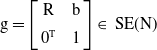 \begin{equation}\mathrm{g}=\left[\begin{array}{c@{\quad}c} \mathrm{R} & \mathrm{b}\\[5pt] 0^{\mathrm{T}} & 1 \end{array}\right]\in \text{ SE}(\mathrm{N})\end{equation}
where $\mathrm{R}\in \mathrm{SO}(\mathrm{N})$
is the rotation matrix and
$\mathrm{R}\in \mathrm{SO}(\mathrm{N})$
is the rotation matrix and $\mathrm{b}\in \mathrm{R}^{\mathrm{N}}$
is the position vector. N for 2D cases is 2, and for 3D cases it is 3. The distance between two frames, which are illustrated by
$\mathrm{b}\in \mathrm{R}^{\mathrm{N}}$
is the position vector. N for 2D cases is 2, and for 3D cases it is 3. The distance between two frames, which are illustrated by $\mathrm{g}_{1}$
and
$\mathrm{g}_{1}$
and $\mathrm{g}_{2}$
, can be expressed as follows:
$\mathrm{g}_{2}$
, can be expressed as follows:
 \begin{equation}\mathrm{D}(\mathrm{g}_{1},\mathrm{g}_{2})=\sqrt{ \left\| \mathrm{b}_{1}-\mathrm{b}_{2}\right\| ^{2}+{\mathrm{L}^{2}} \left\| \log {\mathrm{R}_{1}}^{\mathrm{T}}\mathrm{R}_{2}\right\| ^{2}}\end{equation}
where $\| \cdot \|$
is the Euclidean norm. L is a parameter mainly introduced to match the units of the squared terms. In this article, the value of L = 0.1 was used. Readers are referred to Park’s paper [Reference Park39] for more information.
$\| \cdot \|$
is the Euclidean norm. L is a parameter mainly introduced to match the units of the squared terms. In this article, the value of L = 0.1 was used. Readers are referred to Park’s paper [Reference Park39] for more information.


