


1 INTRODUCTION
1.1 Marine Reservoir Ages and the Marine Calibration Curves
In a world unperturbed by anthropogenic emissions, the concentration of 14C in the oceans is always depleted compared with the atmosphere. High frequency variations present in the atmospheric 14C signal are also smoothed out in marine environments. The amount of marine 14C depletion is variable over time, as well as being dependent upon the location and depth of the water. For a specific location and calendar age θ cal yr BP, we quantify the level of 14C depletion using the marine reservoir age (MRA), denoted as R Location (θ). The MRA defines the difference, at calendar age θ cal yr BP, between the radiocarbon age of dissolved inorganic carbon in the mixed ocean surface layer at that location, and the radiocarbon age of CO2 in the Northern Hemispheric (NH) atmosphere. Higher MRA values mean there is a greater level of 14C depletion in the ocean, and a larger disequilibrium with the atmosphere, at that location and time.
There are multiple complex factors affecting the MRA (Bard Reference Bard1988) but they can be roughly split into those acting at a global-scale, and more localized effects. The global-scale factors include atmospheric CO2 concentration and 14C production changes, and large-scale changes to ocean circulation and air-sea gas exchange rates. Additional global-scale effects include the smoothed and delayed response of the surface oceans, when compared with the more rapid atmospheric response, to variations in 14C production rate which occurs as a consequence of surface waters mixing with the extremely large carbon reservoir in the deeper ocean (Levin and Hesshaimer Reference Levin and Hesshaimer2000). The more local effects, which would influence the MRA in a smaller neighborhood, might include regional sea-ice, regional winds, water depth, and local upwelling (Key Reference Key2001; Reimer and Reimer Reference Reimer and Reimer2001; Key et al. Reference Key, Kozyr, Sabine, Lee, Wanninkhof, Bullister, Feely, Millero, Mordy and Peng2004; Toggweiler et al. Reference Toggweiler, Druffel, Key and Galbraith2019). We can therefore partition our location specific, and time dependent, MRA estimate into:
 $${R^{Location}}\left( \theta \right) = {R^{GlobalAv}}\left( \theta \right) + {\rm{\Delta }}{R^{Location}}\left( \theta \right),$$
where R GlobalAv (θ) captures the global-scale MRA effects and the oceanic smoothing of high-frequency 14C production rate changes; and ΔR Location (θ) the local depletion factors (Bard Reference Bard1988; Stuiver and Braziunas Reference Stuiver and Braziunas1993; Heaton et al. Reference Heaton, Köhler, Butzin, Bard, Reimer, Austin, Bronk-Ramsey, Grootes, Hughen, Kromer, Reimer, Adkins, Burke, Cook, Olsen and Skinner2020).
The goal of the Marine20 calibration curve (Heaton et al. Reference Heaton, Köhler, Butzin, Bard, Reimer, Austin, Bronk-Ramsey, Grootes, Hughen, Kromer, Reimer, Adkins, Burke, Cook, Olsen and Skinner2020) is to provide a “best estimate” of the global-scale surface water 14C concentration in the open ocean that has factored out R GlobalAv (θ). The Marine20 curve therefore aims to provide a global-scale baseline to remove the large-scale effects on the surface ocean MRA of the global palaeoclimatic and carbon cycle variables on which we have current knowledge; and critically also to account for the inherent oceanic smoothing of the high-frequency atmospheric 14C variation.
Oceanic 14C levels vary more smoothly than the atmosphere not only in terms of Δ14C (vs. calendar age), but also in terms of radiocarbon age (vs. calendar age). Representing this oceanic smoothing of the atmospheric variations in the radiocarbon age over time is one of the primary reasons why a product such as Marine20 is useful for calibration and interpretation of marine 14C samples. To obtain this radiocarbon age smoothing requires careful modeling of the MRA. The value of R GlobalAv (θ) varies rapidly to account for periods when the atmospheric radiocarbon age has fluctuated in response to a 14C production change, but the ocean’s radiocarbon age has not. Such radiocarbon age smoothing cannot be achieved by modeling with a constant MRA, see Section 5.1.1. While a constant MRA (equivalent to a constant proportion of the carbon being 14C-free) will reduce the size of oscillations in the Δ14C vs. calendar age, in terms of radiocarbon age vs. calendar age it equates to applying a constant offset from the atmospheric equivalent, leaving the size of radiocarbon age vs. calendar age oscillations the same. In this paper, when we discuss the damping of atmospheric signal, we will always be referring to the smoothing of the oscillations in radiocarbon age vs. calendar time unless stated otherwise.
The resultant global-scale Marine20 summary is intended to aid the research of two groups of marine 14C users—those archaeologists and environmental scientists wishing to calibrate 14C samples of unknown age that have obtained their carbon from the marine environment; and those palaeoceanographers wishing to understand additional MRA changes and hence finer-scaled behaviour of the carbon cycle and oceans over space and time.
We stress that all the Marine calibration curves are only intended for the open oceans, in combination with a ΔR atlas. Calibrating 14C samples from closed seas and large lakes, or understanding 14C variation in such locations, is considerably more challenging. We discuss the calibration of such samples in Section 5.1.3.
Notation: Each update of the Marine calibration curve generates new estimates for R GlobalAv (θ) and consequently will require updates to ΔR Location (θ). We now use a subscript to denote the curve-specific values so that, e.g., R 20 GlobalAv (θ) and ΔR 20(θ) refer to the global-scale and the additional local-scale estimates corresponding to the Marine20 curve (Heaton et al. Reference Heaton, Köhler, Butzin, Bard, Reimer, Austin, Bronk-Ramsey, Grootes, Hughen, Kromer, Reimer, Adkins, Burke, Cook, Olsen and Skinner2020); and R 13 GlobalAv (θ) and ΔR 13(θ) the Marine13 values (Reimer et al. Reference Reimer, Bard, Bayliss, Beck, Blackwell, Bronk Ramsey, Buck, Cheng, Edwards, Friedrich, Grootes, Guilderson, Haflidason, Hajdas, Hatté, Heaton, Hoffmann, Hogg, Hughen, Kaiser, Kromer, Manning, Niu, Reimer, Richards, Scott, Southon, Staff, Turney and van der Plicht2013). For ease of reading, we drop the location superscript in ΔR Location where it is not required.
1.2 Intention of this Response to the Community
Following the release of the Marine20 curve (Heaton et al. Reference Heaton, Köhler, Butzin, Bard, Reimer, Austin, Bronk-Ramsey, Grootes, Hughen, Kromer, Reimer, Adkins, Burke, Cook, Olsen and Skinner2020) we received multiple requests from the 14C community asking if we could provide a more intuitive description of the product aimed at the lay-reader. Motivated by these requests, we have provided this short note.
To guide our response, we collated a set of questions from both archaeological and environmental science users through Dr. Irka Hajdas, Dr. Christine Hatté, and Prof. Tim Jull. These have then been grouped thematically to form the structure of this paper. We split our responses into four sections. Section 2 addresses questions regarding the various uses of Marine calibration curves; and provides a brief summary as to why using Marine20 provides a benefit over Marine13. Section 3 regards the specific construction of the Marine20 curve, and explains the similarities and differences between Marine20 and the earlier Marine calibration curves such as Marine04, 09, and 13 (Hughen et al. Reference Hughen, Baillie, Bard, Beck, Bertrand, Blackwell, Buck, Burr, Cutler, Damon, Edwards, Fairbanks, Friedrich, Guilderson, Kromer, McCormac, Manning, Bronk Ramsey, Reimer, Reimer, Remmele, Southon, Stuiver, Talamo, Taylor, van der Plicht and Weyhenmeyer2004b; Reimer et al. Reference Reimer, Baillie, Bard, Bayliss, Beck, Blackwell, Bronk Ramsey, Buck, Burr, Edwards, Friedrich, Grootes, Guilderson, Hajdas, Heaton, Hogg, Hughen, Kaiser, Kromer, McCormac, Manning, Reimer, Richards, Southon, Talamo, Turney, van der Plicht and Weyhenmeyer2009, Reference Reimer, Bard, Bayliss, Beck, Blackwell, Bronk Ramsey, Buck, Cheng, Edwards, Friedrich, Grootes, Guilderson, Haflidason, Hajdas, Hatté, Heaton, Hoffmann, Hogg, Hughen, Kaiser, Kromer, Manning, Niu, Reimer, Richards, Scott, Southon, Staff, Turney and van der Plicht2013). Section 4 concentrates on the implications for users and provides worked examples of how to estimate ΔR(θ) for a particular location using the Marine20 curve and how to then calibrate 14C determinations. It is key to understand that these ΔR(θ) values must be updated to ΔR 20(θ) when using the Marine20 calibration curve. Finally in Section 5, we address further miscellaneous questions on the use of Marine20 which the community have raised.
Some of our responses overlap with information given in the Marine20 paper (Heaton et al. Reference Heaton, Köhler, Butzin, Bard, Reimer, Austin, Bronk-Ramsey, Grootes, Hughen, Kromer, Reimer, Adkins, Burke, Cook, Olsen and Skinner2020). However, here we have tried to provide a more intuitive understanding—minimizing technical detail but keeping the essential ideas. We hope this approach is more accessible for the highly diverse range of potential Marine20 users. Those readers seeking greater modeling details should refer to Heaton et al. (Reference Heaton, Köhler, Butzin, Bard, Reimer, Austin, Bronk-Ramsey, Grootes, Hughen, Kromer, Reimer, Adkins, Burke, Cook, Olsen and Skinner2020).
2 WHAT IS MARINE20 FOR? WHY IS IT AN IMPROVEMENT OVER MARINE13?
2.1 Uses of Marine20
Broadly speaking, Marine20 has two groups of users: those who have known-age marine 14C samples who want to understand variations in oceanic 14C depletion and hence investigate potential changes to the carbon cycle; and those seeking to calibrate marine 14C samples. The needs of these two user groups are strongly linked.
2.1.1 To study MRA changes beyond those caused by oceanic smoothing of atmospheric 14C and global palaeoclimatic variables
Palaeoceanographers are typically interested in understanding the spatial and temporal variations in MRA using 14C determinations for which they also have independent calendar age estimates. Estimates of region-specific MRA variations that enable insight into potential carbon cycle changes can be most usefully obtained by considering the offset between the Marine20 curve and their 14C data. This offset is ΔR 20(θ).
The ocean and the atmosphere respond differently to variation in 14C production rates. Changes in atmospheric 14C levels typically take time to be transferred to the surface ocean and are also significantly damped (Druffel and Suess Reference Druffel and Suess1983; Grottoli and Eakin Reference Grottoli and Eakin2007; Komugabe-Dixson et al. Reference Komugabe-Dixson, Fallon, Eggins and Thresher2016; Bard and Heaton Reference Bard and Heaton2021). This is a consequence of mixing between the surface layer of the ocean and the extremely large carbon reservoir in deeper ocean layers (in total, during late-Holocene/pre-industrial times, the ocean contained ∼ 60 times more carbon than the atmosphere), and the slow rate of air-sea CO2 equilibration (Grottoli and Eakin Reference Grottoli and Eakin2007; Skinner and Bard Reference Skinner and Bard2022). The resultant smoothing, and phase shift, of changes in atmospheric 14C levels that is inherent to the surface ocean causes considerable high-frequency variation in the overall MRA at any site—whereby atmospheric 14C levels have changed but the ocean is still in the process of responding/equilibrating—see Figure 1 for a model-based illustration of the effect on overall MRA of this ocean smoothing.
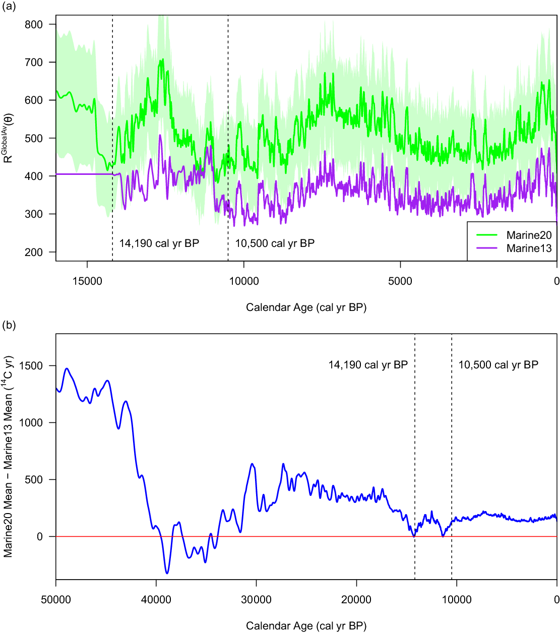
Figure 1 Panel (a) The mean R20 GlobalAv(θ) estimate of Marine20 (green, shown with 2σ-intervals) vs. the mean R13 GlobalAv(θ) of Marine13 (purple) from 15,000–0 cal yr BP. The vertical lines (at 14,190 and 10,500 cal yr BP) denote the breakpoints between the three different methods employed to construct the Marine13 curve. These plotted curves should be thought of as providing estimates for global-scale changes in MRA over time rather than a specific “global-average” MRA. Since the overall 14C depletion in any specific location is offset from these values by ΔR, it is the shape of RGlobalAv(θ) which is important for inference rather than their absolute values. From 10,500–0 cal yr BP, the shape of R20 GlobalAv(θ) remains similar to R13 GlobalAv(θ) indicating estimates of global-scale MRA changes and the overall estimates of 14C depletion at a specific oceanic site do not change substantially with Marine20 in this period. Further back in time, estimated changes in depletion are however significant. Panel (b) The offset between the mean of the Marine20 curve and the Marine13 curve. From 10,500–0 cal yr BP, the offset remains approximately constant over time as, during this time period, neither the atmospheric 14C estimate (IntCal13 vs. IntCal20) nor the global-scale effects (R13 GlobalAv(θ) vs. R20 GlobalAv(θ)) diverge. Further back in time, from 55,000–10,500 cal yr BP the differences between Marine20 and Marine13 are due to the combination of improvements in the modeling of R20 GlobalAv(θ) and improved knowledge of atmospheric 14C levels available in IntCal20.
These high-frequency changes in overall MRA, that occur solely due to oceanic smoothing of atmospheric 14C production, are not however of primary interest for those aiming to understanding carbon cycle changes. In fact, they are typically nuisance variables that act as confounders, hindering useful inference about carbon cycle changes when comparing observed 14C samples across oceanic sites or over time. Ideally, we would wish to remove, or factor out, these smoothing-based (nuisance) variations in overall MRA so that we can study and discover other, more scientifically interesting, causes for changes in oceanic 14C depletion levels more easily.
Equally, we would wish to factor out those confounding changes in overall MRA that are due to changes in global-scale palaeoclimate variables, for example those due to variations in CO2 concentration (Köhler et al. Reference Köhler, Nehrbass-Ahles, Schmitt, Stocker and Fischer2017), wind speed (Petit et al. Reference Petit, Mourner, Jouzel, Korotkevich, Kotlyakov and Lorius1990; McGee et al. Reference McGee, Broecker and Winckler2010; Kohfeld et al. Reference Kohfeld, Graham, de Boer, Sime, Wolff, Le Quéré and Bopp2013; Kageyama et al. Reference Kageyama, Harrison, Kapsch, Lofverstrom, Lora, Mikolajewicz, Sherriff-Tadano, Vadsaria, Abe-Ouchi, Bouttes, Chandan, Gregoire, Ivanovic, Izumi, LeGrande, Lhardy, Lohmann, Morozova, Ohgaito, Paul, Peltier, Poulsen, Quiquet, Roche, Shi, Tierney, Valdes, Volodin and Zhu2021), or in the Atlantic meridional overturning circulation (AMOC) (Böhm et al. Reference Böhm, Lippold, Gutjahr, Frank, Blaser, Antz, Fohlmeister, Frank, Andersen and Deininger2015; Henry et al. Reference Henry, McManus, Curry, Roberts, Piotrowski and Keigwin2016; Oka et al. Reference Oka, Abe-Ouchi, Sherriff-Tadano, Yokoyama, Kawamura and Hasumi2021) and wider carbon cycle (Bauska et al. Reference Bauska, Marcott and Brook2021). Factoring out the effect of these variables allows us to better compare changes in the carbon cycle over time between different oceanic locations, especially when we do not have contemporaneous 14C samples from all our sites. After having factored out the effect of global-scale variables, if we can identify that further MRA changes have occurred in one location, but not another, then this suggests localized carbon cycle variations.
Given known-age marine 14C samples from a specific location, both the inherent oceanic smoothing and global-scale confounders in overall MRA can be factored out by studying ΔR 20(θ), the offset of the specific samples to the Marine20 curve. Marine20 accounts for the damping of fine-scale atmospheric 14C variation which occurs in the oceans, and also incorporates the global-scale MRA effects. Consequently, studying the ΔR 20(θ) offset allows the disentangling of any confounding MRA changes that are due to global palaeoclimatic variables and the oceanic smoothing of rapid atmospheric 14C changes. Changes in ΔR 20(θ) over both space and time can therefore help to inform on important changes in localized oceanic conditions.
This approach to understanding variations in the carbon cycle, in particular those concerning ocean circulation and ventilation, by estimating changes in ΔR(θ) has been employed in multiple marine locations. Examples include the Southern Ocean (van Beek et al. Reference van Beek, Reyss, Paterne, Gersonde, van der Loeff and Kuhn2002); the Atlantic Ocean (Waelbroeck et al. Reference Waelbroeck, Lougheed, Vazquez Riveiros, Missiaen, Pedro, Dokken, Hajdas, Wacker, Abbott and Dumoulin2019); tropical Atlantic (Hughen et al. Reference Hughen, Lehman, Southon, Overpeck, Marchal, Herring and Turnbull2004a); the North Atlantic and Norwegian Seas (Bondevik et al. Reference Bondevik, Mangerud, Birks, Gulliksen and Reimer2006; Ascough et al. Reference Ascough, Cook and Dugmore2009; Muschitiello et al. Reference Muschitiello, D’Andrea, Schmittner, Heaton, Balascio, deRoberts, Caffee, Woodruff, Welten, Skinner, Simon and Dokken2019; Brendryen et al. Reference Brendryen, Haflidason, Yokoyama, Haaga and Hannisdal2020); the Gulf of Oman (Lindauer et al. Reference Lindauer, Santos, Steinhof, Yousif, Phillips, Jasim, Uerpmann and Hinderer2017); and the Florida Keys reef tract (Toth et al. Reference Toth, Cheng, Edwards, Ashe and Richey2017). Research has also been undertaken to understand ΔR(θ) variability, and its potential causes, in a range of Pacific Ocean locations including the Gulf of Panamá (Toth et al. Reference Toth, Aronson, Cheng and Edwards2015); off the coast of Peru and Chile (Ortlieb et al. Reference Ortlieb, Vargas and Saliège2011; Carré et al. Reference Carré, Jackson, Maldonado, Chase and Sachs2016; Latorre et al. Reference Latorre, De Pol-Holz, Carter and Santoro2017); the South China Sea (Yu et al. Reference Yu, Hua, Zhao, Hodge, Fink and Barbetti2010; Hirabayashi et al. Reference Hirabayashi, Yokoyama, Suzuki, Esat, Miyairi, Aze, Siringan and Maeda2019; Hua et al. Reference Hua, Ulm, Yu, Clark, Nothdurft, Leonard, Pandolfi, Jacobsen and Zhao2020); and the South Pacific, including the central South Pacific Gyre (Petchey Reference Petchey2020), New Zealand (Petchey and Schmid Reference Petchey and Schmid2020), Papua New Guinea (McGregor et al. Reference McGregor, Gagan, McCulloch, Hodge and Mortimer2008), Vanuatu and the Solomon Islands (Burr et al. Reference Burr, Vance Haynes, Shen, Taylor, Chang, Beck, Nguyen and Zhou2015), the Great Barrier Reef (Hua et al. Reference Hua, Webb, Zhao, Nothdurft, Lybolt, Price and Opdyke2015, Reference Hua, Ulm, Yu, Clark, Nothdurft, Leonard, Pandolfi, Jacobsen and Zhao2020), and the South Tasman Sea (Komugabe-Dixson et al. Reference Komugabe-Dixson, Fallon, Eggins and Thresher2016). In some locations, changes over time in the observed value of ΔR(θ) appear to be relatively small, while in other regions larger temporal variations are seen. Readers should note that the estimates of changes in ΔR(θ) over time in these papers relate to previous versions of the Marine calibration curve. They will need updating in light of the improved Marine20—although we expect that inference on variations in ΔR(θ) in the Holocene will remain similar due to the relatively limited changes in the Marine13 and Marine20 estimates (beyond a constant offset) in this time period.
We also note that the global-scale estimates of MRA, R 20 GlobalAv (θ), that are produced by Marine20 are also useful for those using directly-paired atmospheric and marine 14C samples to estimate variations in overall MRA (e.g., Bard et al. Reference Bard, Arnold, Mangerud, Paterne, Labeyrie, Duprat, Mélières, Sønstegaard and Duplessy1994; Siani et al. Reference Siani, Paterne, Michel, Sulpizio, Sbrana, Arnold and Haddad2001, Reference Siani, Michel, De Pol-Holz, DeVries, Lamy, Carel, Isguder, Dewilde and Lourantou2013; Skinner et al. Reference Skinner, Primeau, Freeman, de la Fuente, Goodwin, Gottschalk, Huang, McCave, Noble and Scrivner2017; Telesiński et al. Reference Telesiński, Ezat, Muschitiello, Bauch and Spielhagen2021). These studies, looking at direct ocean-atmospheric 14C age differences R Location (θ), are somewhat hampered when seeking to infer which changes are due to variations in CO2 levels or 14C production rates; and which are due to localized ocean ventilation changes. Separating out these effects can be improved by comparing the overall changes they observe in R Location (θ) to our Marine20 estimate of R 20 GlobalAv (θ).
2.1.2 To calibrate new marine 14C samples
Those seeking to calibrate new marine 14C determinations from a specific location need a local marine 14C calibration curve. Currently, we have insufficient knowledge about the local factors affecting MRA to accurately model region-specific calibration curves. For most locations, we also cannot obtain good data-based estimates of ΔR(θ) over prolonged periods—which could otherwise be used to create a local marine calibration curve—due to a sparsity of 14C data for which calendar ages are independently known (see Section 2.1.3 for more details on regional calibration curves).
If we wish to calibrate marine 14C samples from a particular location, we are therefore required to make a significant simplification. This simplification, used since the first Marine calibration curve (Stuiver et al. Reference Stuiver, Pearson and Braziunas1986), is to model the localized ΔR(θ) in the location of interest as being approximately constant, or at most to vary relatively slowly, over time. This simplification permits us to obtain an estimate for a local marine calibration curve using Marine20 in combination with known-age 14C samples, or paired marine and terrestrial 14C samples, from the site of interest.
We recognize that this simplification is a very significant approximation and lies at odds with Section 2.1.1. In practice, we should expect ΔR(θ) to vary over time in any location due to changes in local ocean circulation or other localized factors. The scale of these ΔR(θ) changes over time will vary dependent upon the location, as shown by the various research in Section 2.1.1. In certain locations, variation over time will be small and so the approximation will be good; in others there may have been larger changes in ΔR(θ) over time and treating it as approximately constant will be a much coarser approximation. However, such a simplification does permit the user 14C community to implement a standardised approach to marine calibration that can be used until our knowledge improves and reliable regional marine calibration curves become available. If possible, we always recommend users try and use an estimate of ΔR(θ) from a calendar age that is as close to the age of their specific samples as possible to limit the impact of potential ΔR(θ) changes.
If we are willing to assume that, in our ocean location of interest, the additional local depletion effects ΔR(θ) are approximately constant over time, then we can use known-age 14C data from that location to estimate a constant ΔR. In the case of Marine20 this is denoted ΔR 20. Such a ΔR 20 can then be used to adjust Marine20 and provide a localized calibration curve. Ideally, one would obtain this estimate of ΔR 20 based on 14C samples of similar calendar age to that which one is calibrating—for example, if one has an archaeological site with tightly linked (contemporaneous) shells and charcoal, or paired U-Th and 14C dates on the same ocean coral. However, if it is not possible to obtain an estimate of ΔR 20 using data of a similar calendar age to that one wishes to calibrate, one must rely upon 14C data from the recent past. A maintained database to enable estimation of regional ΔR 20 based on such recent samples is provided at http://calib.org/marine/ (Reimer and Reimer Reference Reimer and Reimer2001).
During the Holocene, to enable 14C calibration, a simplification of an approximately constant ΔR(θ) over time is perhaps justifiable for a broader range of ocean locations due to the relatively stable global climate. However, for samples that come from before the onset of the Holocene, such a simplification certainly cannot be justified at higher latitudes (outside ca. 40°S–40°N). During glacial periods, these high latitude regions may have seen localized sea-ice cover, strong winds, and ocean circulation changes that could have had very significant additional short-term effects on ΔR(θ) (Butzin et al. Reference Butzin, Prange and Lohmann2005; Völker and Köhler Reference Völker and Köhler2013). Consequently, in these polar regions, the assumption of a constant ΔR(θ) extending into glacial stadials is inappropriate (Butzin et al. Reference Butzin, Köhler and Lohmann2017). We do not recommend the use of Marine20, with a constant ΔR 20 estimated from Holocene samples, to calibrate 14C samples from polar regions (outside ca. 40°S–40°N) that are older than ca. 11.5 cal kyr BP.
This latitudinal polar divide (of 40°S–40°N) is based on the geometry of low- versus high-latitudinal areas in the BICYCLE model. Simulations with the three-dimensional LSG ocean general circulation model suggest that temporal changes in the presence of sea ice may have the largest influence on ΔR. In regions where sea ice formation can be excluded, Marine20 might still be applicable outside the stated low-latitudinal core area, but should be done so with great caution. We also do not provide an exact date as to when significant changes in ΔR(θ) are likely to have occurred in polar regions. These decisions should be made and justified by the calibration user, drawing on various lines of palaeoclimatic or proxy evidence on the extent of localized sea-ice they may have.
Crucially, this caution regarding the unsuitability for polar calibration in glacial periods is equally valid, if not more so, for any of the earlier Marine calibration curves provided by the IntCal group (e.g., Hughen et al. Reference Hughen, Baillie, Bard, Beck, Bertrand, Blackwell, Buck, Burr, Cutler, Damon, Edwards, Fairbanks, Friedrich, Guilderson, Kromer, McCormac, Manning, Bronk Ramsey, Reimer, Reimer, Remmele, Southon, Stuiver, Talamo, Taylor, van der Plicht and Weyhenmeyer2004b; Reimer et al. Reference Reimer, Baillie, Bard, Bayliss, Beck, Blackwell, Bronk Ramsey, Buck, Burr, Edwards, Friedrich, Grootes, Guilderson, Hajdas, Heaton, Hogg, Hughen, Kaiser, Kromer, McCormac, Manning, Reimer, Richards, Southon, Talamo, Turney, van der Plicht and Weyhenmeyer2009, Reference Reimer, Bard, Bayliss, Beck, Blackwell, Bronk Ramsey, Buck, Cheng, Edwards, Friedrich, Grootes, Guilderson, Haflidason, Hajdas, Hatté, Heaton, Hoffmann, Hogg, Hughen, Kaiser, Kromer, Manning, Niu, Reimer, Richards, Scott, Southon, Staff, Turney and van der Plicht2013). The use of Marine20, or any of the earlier Marine calibration curves, using a constant (Holocene-based) ΔR is likely to significantly underestimate the calendar age uncertainty of glacial-period polar oceanic 14C samples and introduce biases, providing calendar age estimates that may be substantially older than the true age of the 14C sample. See Section 2.1.6 and Heaton et al. (Reference Heaton, Butzin, Bard, Bronk Ramsey, Hughen, Köhler and Reimer2022) for further advice on calibration of polar marine 14C samples.
2.1.3 Calibration using data-based regional marine calibration curves
As explained above, in all marine locations, the value of ΔR(θ) will, to a greater or lesser extent, change over time. All users should therefore be aware of the current limitations of using a constant-adjusted Marine20 (or any earlier Marine curve) when calibrating marine 14C samples and should treat their calendar age estimates with caution accordingly, especially in marine regions where they think local hydrographic conditions will have changed significantly.
The range of recent research, described in Section 2.1.1, that uses 14C samples to provide insight into the scale of changes to ΔR(θ) over time has the potential to enable the creation of regional, data-based, marine calibration curves in some selected locations. Production of such regional curves is however extremely challenging due to the typical sparsity of available 14C marine samples over long time periods, as well as the difficulty in obtaining independent calendar age estimates for them. This is particularly an issue if we wish to create calibration curves which extend far into our past. There are also significant unanswered questions regarding the area over which such observational 14C marine data might reasonably be combined into a single regional curve, and similarly the extent of the spatial neighborhood in which any consequent regional marine curve might be applicable for calibration.
Examples of research on changes in ΔR(θ) where, due to the volume of 14C data from the region that is available, individuals have begun to propose and create regional data-based marine calibration curves covering more prolonged periods include the North Atlantic (Skinner et al. Reference Skinner, Muschitiello and Scrivner2019; Waelbroeck et al. Reference Waelbroeck, Lougheed, Vazquez Riveiros, Missiaen, Pedro, Dokken, Hajdas, Wacker, Abbott and Dumoulin2019), the Norwegian Sea (Muschitiello et al. Reference Muschitiello, D’Andrea, Schmittner, Heaton, Balascio, deRoberts, Caffee, Woodruff, Welten, Skinner, Simon and Dokken2019), and South Florida (Toth et al. Reference Toth, Cheng, Edwards, Ashe and Richey2017). In the Pacific, there is also the Gulf of Panamá (Toth et al. Reference Toth, Aronson, Cheng and Edwards2015), New Zealand (Petchey and Schmid Reference Petchey and Schmid2020), the Great Barrier Reef and the South China Sea (Hua et al. Reference Hua, Ulm, Yu, Clark, Nothdurft, Leonard, Pandolfi, Jacobsen and Zhao2020).
We do not feel able to endorse specific regional calibration curve products but we note that, for some 14C users, these regional marine curves may be appropriate for calibration. As our knowledge and data improve, we expect that more reliable, and more precise, regional calibration curves will become available. However, where ΔR(θ) is unknown, approximations and simplifications are currently still required for most 14C users.
2.2 Why is Marine20 an Improvement over Marine13?
Most simply, Marine20 aims to offer a substantial improvement in the modeling and estimation of the global-scale 14C depletion effects [i.e., R 20 GlobalAv (θ)] compared to the R 13 GlobalAv (θ) estimate used in Marine13. This is achieved by transient application of the carbon cycle model BICYCLE (Köhler and Fischer Reference Köhler and Fischer2004, Reference Köhler and Fischer2006; Köhler et al. Reference Köhler, Fischer, Munhoven and Zeebe2005, Reference Köhler, Muscheler and Fischer2006) to estimate the ocean’s 14C levels. BICYCLE is able to incorporate important time-dependent changes in the global carbon cycle. This was not possible with the box model used for Marine13 (Oeschger et al. Reference Oeschger, Siegenthaler, Schotterer and Gugelmann1975). The improvements in Marine20 are mainly seen in the period from 55,000–10,500 cal yr BP, in particular from 55,000–14,190 cal yr BP. There are however also some differences in the implementation of the Marine20 model compared to the Marine13 box model for the period 10,500–0 cal yr BP. See Figure 1a and Figure 2.

Figure 2 Plot of the mean Marine20 (BICYCLE-based) global-scale estimate of R 20 GlobalAv (θ), shown as green-solid line, against the LSG OGCM estimate of the overall MRA at three specific locations under its GS scenario and the LSG OGCM average under the GS scenario from 50°S–50°N. This GS scenario is intended to represent a glacial scenario (Sarnthein et al. Reference Sarnthein, Gersonde, Niebler, Pflaumann, Spielhagen, Thiede, Wefer and Weinelt2003; Butzin et al. Reference Butzin, Heaton, Köhler and Lohmann2020) although is not transient in climate. Note that the plotted LSG OGCM estimates include their corresponding ΔR term. As we can shift the Marine20 estimate in each location according to a local ΔR 20 estimate, it is the relative shapes of the curves (rather than the offsets) which are of primary relevance for inference. We also show the Marine13 estimate R 13 GlobalAv (θ) in purple for comparison. (Please see online version for color figures.)
We know that from 55,000–10,500 cal yr BP there have been significant changes in global CO2 concentration, related to substantial changes to the carbon cycle, as well as differences in global-average wind speeds compared with the recent past (Petit et al. Reference Petit, Mourner, Jouzel, Korotkevich, Kotlyakov and Lorius1990; McGee et al. Reference McGee, Broecker and Winckler2010; Böhm et al. Reference Böhm, Lippold, Gutjahr, Frank, Blaser, Antz, Fohlmeister, Frank, Andersen and Deininger2015; Köhler et al. Reference Köhler, Nehrbass-Ahles, Schmitt, Stocker and Fischer2017). We also know that these factors must have affected the MRA. However, it was not possible to include these changes in the computational modeling of Marine13 (Reimer et al. Reference Reimer, Bard, Bayliss, Beck, Blackwell, Bronk Ramsey, Buck, Cheng, Edwards, Friedrich, Grootes, Guilderson, Haflidason, Hajdas, Hatté, Heaton, Hoffmann, Hogg, Hughen, Kaiser, Kromer, Manning, Niu, Reimer, Richards, Scott, Southon, Staff, Turney and van der Plicht2013). From 14,190–10,500 cal yr BP, Marine13 used a small set of marine records from tropical and subtropical locations to try and incorporate these changes from observational records. However, the Marine13 curve made no attempt to model global-scale changes in MRA from 55,000–14,190 cal yr BP. Marine13 set R 13 GlobalAv (θ) to be constant 405 14C yrs throughout this period (Figures 1a and 2).
When using Marine13, any MRA changes from 55,000–14,190 cal yr BP had to be entirely incorporated in the local ΔR 13(θ), conflating global-scale and localized effects. If you were calibrating a 14C sample and did not know how ΔR 13(θ) changed over time, then you still had to model it as constant. This meant, with Marine13, you were effectively assuming there had been no variation in oceanic 14C depletion from 55,000–14,190 cal yr BP. This is clearly incorrect, not least as the substantial changes in atmospheric 14C levels (Reimer et al. Reference Reimer, Austin, Bard, Bayliss, Blackwell, Ramsey, Butzin, Cheng, Edwards, Friedrich, Grootes, Guilderson, Hajdas, Heaton, Hogg, Hughen, Kromer, Manning, Muscheler, Palmer, Pearson, van der Plicht, Reimer, Richards, Scott, Southon, Turney, Wacker, Adolphi, Büntgen, Capano, Fahrni, Fogtmann-Schulz, Friedrich, Köhler, Kudsk, Miyake, Olsen, Reinig, Sakamoto, Sookdeo and Talamo2020) would have affected the MRA.
Marine20 offers an improvement from 55,000–10,500 cal yr BP by incorporating, through usage of the BICYCLE model (Köhler and Fischer Reference Köhler and Fischer2004, Reference Köhler and Fischer2006; Köhler et al. Reference Köhler, Fischer, Munhoven and Zeebe2005, Reference Köhler, Muscheler and Fischer2006), as many of the known, and shared, global-scale palaeoclimate and carbon cycle changes that might influence oceanic 14C depletion as currently possible. These large-scale carbon cycle changes are included in our estimate of R 20 GlobalAv (θ), and hence also the Marine20 curve (Figures 1 and 2). This enables better separation of global and local effects. Marine20 aims to model the effect of the changing global CO2 concentration, atmospheric 14C, wind speed, and basic carbon cycle changes in ocean circulation. Consequently, when using Marine20 we hope to have better accounted for the known effects of the global carbon cycle, and the damping of the atmospheric 14C variations inherent to the ocean environment.
For the 10,500–0 cal yr BP period, Marine20 also aims to provide some small improvements in its estimate of R 20 GlobalAv (θ), and hence in the calibration curve, compared to the previous R 13 GlobalAv (θ) and Marine13 (see Figure 1). These are primarily due to an increased understanding of atmospheric 14C production (since for Marine20 the model is forced by the improved IntCal20 curve rather than IntCal13) and the incorporation of more minor changes in global CO2 concentration. Note that, when comparing Marine20 [and R 20 GlobalAv (θ)] against Marine13 [and R 13 GlobalAv (θ)] it is their relative changes over time which are important, not their absolute values. The curves aim to represent global-scale temporal effects, rather than a specific spatial average. The ∼150 14C yrs offset between the Marine20 and Marine13 versions in the recent past is not therefore of direct relevance for comparisons. This offset will be accounted for in the changes from ΔR 13 to ΔR 20. We discuss this further in Section 3.1.3.
2.3 Why Does This Marine20 Improvement Matter for a 14C User?
For those seeking to obtain spatial understanding of MRAs to study the carbon cycle, the use of Marine20 makes it easier to compare MRA estimates in different locations—in particular, when the reference 14C data are not all of the same calendar age. For those aiming to understand more detailed temporal MRA changes, comparison against Marine20 allows one to factor out the oceanic smoothing of rapid changes in atmospheric 14C production rate and remove the effects of the global carbon cycle—any further MRA changes can therefore be identified as due to other time-varying factors. Conversely, a user studying spatial and temporal variations in the offset between the Marine13 curve and 14C samples during the period from 55,000–14,190 cal yr BP could not disentangle local ocean reservoir changes from globally-shared effects. This hindered useful inference when comparing marine 14C samples from the glacial period against Marine13 and earlier marine calibration curves. With these previous marine calibration curves, users had to estimate themselves whether the changes they saw in R Location (θ) in the last glacial were due to global changes in atmospheric CO2 partial pressure or in wind strength; or whether they were caused by changes in ocean ventilation (e.g., Bard et al. Reference Bard, Arnold, Mangerud, Paterne, Labeyrie, Duprat, Mélières, Sønstegaard and Duplessy1994; Sikes et al. Reference Sikes, Samson, Guilderson and Howard2000; Siani et al. Reference Siani, Paterne, Michel, Sulpizio, Sbrana, Arnold and Haddad2001). This is now addressed by estimating the offset ΔR 20(θ) against Marine20.
For users calibrating new marine 14C samples from a given location, the benefit of Marine20 can be seen by considering the two potential sources of errors when using any marine calibration curve from the IntCal project:
-
a. Error when modeling the global-scale MRA effects R GlobalAv (θ);
-
b. Error in modeling the local MRA effects ΔR(θ) as constant—in any region there are likely to be local factors affecting the MRA which aren't seen on a global level and which change over time, e.g., appearance and disappearance of sea-ice, and short-term local changes in circulation and upwelling.
Since Marine13 modeled R 13 GlobalAv (θ) as constant from 55,000–14,190 cal yr BP, the use of Marine13 for calibration of samples from this period will introduce significant errors of type (a). Conversely, the use of Marine20, with a variable R 20 GlobalAv (θ) that incorporates the effect of known global-scale variables on 14C depletion, will reduce the magnitude of this type of error and so should improve calibration reliability. In the period from 14,190–0 cal yr BP, the differences between using Marine13 and Marine20 will typically be much smaller—so long as one ensures they update the estimate of ΔR 13 to ΔR 20. We note that for both Marine13 and Marine20, potential error of type (b) will remain where there is temporal variation in regional factors that affect the local 14C depletion but not the wider ocean. Without better understanding of regional effects, for which more detailed regional archives will likely be needed as discussed in Section 2.1.3, this type (b) error will remain somewhat irreducible.
3 QUESTIONS ON THE CONSTRUCTION OF MARINE20
3.1 Comparisons of Marine20 with Marine13
3.1.1 Have we changed our approach for Marine20, and if so, why?
The fundamental idea of the marine calibration curve has not changed between Marine20 and the earlier Marine curves. Both Marine20 and Marine13 use, where possible, an ocean-atmosphere computer model to estimate the changes in the MRA at the surface ocean which occur at a global-scale, i.e., R GlobalAv (θ), and simultaneously use this estimate to generate a global-scale oceanic calibration curve which factors out R GlobalAv (θ).
However, for Marine13, and the preceding marine calibration curves, these ocean-atmosphere computer models could not be extended back beyond 10,500 cal yr BP since they were not able to incorporate the carbon cycle and climate changes which are known to have occurred before then (Petit et al. Reference Petit, Mourner, Jouzel, Korotkevich, Kotlyakov and Lorius1990; McGee et al. Reference McGee, Broecker and Winckler2010; Böhm et al. Reference Böhm, Lippold, Gutjahr, Frank, Blaser, Antz, Fohlmeister, Frank, Andersen and Deininger2015; Henry et al. Reference Henry, McManus, Curry, Roberts, Piotrowski and Keigwin2016; Köhler et al. Reference Köhler, Nehrbass-Ahles, Schmitt, Stocker and Fischer2017; Bauska et al. Reference Bauska, Marcott and Brook2021). Significant simplifications were therefore required from 55,000–10,500 cal yr BP. With Marine20, through use of the carbon cycle box model BICYCLE (Köhler et al. Reference Köhler, Muscheler and Fischer2006), we have been able to extend the computational modeling approach back to 55,000 cal yr BP and include more detailed knowledge regarding observed changes in the global carbon cycle. Hopefully, Marine20 therefore incorporates an improved estimate of the global-scale MRA effects which also extends back further in time.
3.1.2 What was done for Marine09 and Marine13?
For both Marine09 (Reimer et al. Reference Reimer, Baillie, Bard, Bayliss, Beck, Blackwell, Bronk Ramsey, Buck, Burr, Edwards, Friedrich, Grootes, Guilderson, Hajdas, Heaton, Hogg, Hughen, Kaiser, Kromer, McCormac, Manning, Reimer, Richards, Southon, Talamo, Turney, van der Plicht and Weyhenmeyer2009) and Marine13 (Reimer et al. Reference Reimer, Bard, Bayliss, Beck, Blackwell, Bronk Ramsey, Buck, Cheng, Edwards, Friedrich, Grootes, Guilderson, Haflidason, Hajdas, Hatté, Heaton, Hoffmann, Hogg, Hughen, Kaiser, Kromer, Manning, Niu, Reimer, Richards, Scott, Southon, Staff, Turney and van der Plicht2013), the curve from 10,500–0 cal yr BP was based upon a simple ocean-atmosphere box-diffusion model (Oeschger et al. Reference Oeschger, Siegenthaler, Schotterer and Gugelmann1975). This box-model approach had been taken since 1986 (Stuiver et al. Reference Stuiver, Pearson and Braziunas1986). The available tree-ring 14C data were used as the atmospheric model input, and parameters for air-sea gas exchange and eddy diffusivity were set to hit pre-bomb 14C targets for the surface and deep ocean. This resulted in an estimate of the global-scale MRA R 13 GlobalAv (θ) (see Figure 1a) that was variable from 10,500–0 cal yr BP. However, in this time period, the variation is relatively small since the climate state was relatively constant, and carbon cycle (atmospheric CO2) changes were minor.
For the portion of the Marine13 curve from 14,190–10,500 cal yr BP, Marine13 was based on a small set of, tropical and subtropical, coral and sediment records. This limited marine data was combined using the same statistical methodology as for IntCal13 (Niu et al. Reference Niu, Heaton, Blackwell and Buck2013) with the mean MRA for each site calculated from the overlap with the tree-rings. From 50,000–14,190 cal yr BP there were no tree-rings for calculating a global-scale MRA so a constant value of 405 14C yrs was applied (Figure 2) even though it was recognized that the use of a constant value wasn’t correct because large global-scale MRA changes must have occurred.
The constant value of 405 14C yrs used for R 13 GlobalAv (θ) from 50,000–14,190 cal yr BP has remained the same since Marine04 (Hughen et al. Reference Hughen, Baillie, Bard, Beck, Bertrand, Blackwell, Buck, Burr, Cutler, Damon, Edwards, Fairbanks, Friedrich, Guilderson, Kromer, McCormac, Manning, Bronk Ramsey, Reimer, Reimer, Remmele, Southon, Stuiver, Talamo, Taylor, van der Plicht and Weyhenmeyer2004b) and was chosen to match the output of the Marine04 box-diffusion model output between AD 1350–1850. This model value is essentially the same as those used for calibrations before IntCal04 by Stuiver et al. (Reference Stuiver, Pearson and Braziunas1986) (409 yr), by Stuiver and Braziunas (Reference Stuiver and Braziunas1993) (402 yr), and Stuiver et al. (Reference Stuiver, Reimer, Bard, Beck, Burr, Hughen, Kromer, McCormac, van der Plicht and Spurk1998) (400 yr). Since the carbon cycle was considerably different pre-Holocene compared with AD 1350–1850, such an estimate of ≈ 400 14C yrs is likely to be highly inappropriate between 50,000–14,190 cal yr BP during the last glaciation.
3.1.3 But has the Marine20 curve not meant that calibration and overall MRA estimates have changed significantly from Marine13 even in the Holocene?
In the Holocene, the global-scale Marine20 curve [and accompanying R 20 GlobalAv (θ)] is offset by ∼150 14C yrs from the Marine13 curve [and corresponding R 13 GlobalAv (θ)]—see Figure 1b. However, this does not mean the estimate for the overall 14C depletion in any specific oceanic location has changed substantially in the time period up until 10,500 cal yr BP.
The R GlobalAv (θ) is poorly named. Rather than denoting the global-average MRA, it is more helpful to consider it as an estimate of global-scale MRA changes. It is the shape of this estimate, and specifically how it varies over time, which is important. As described in Section 1.1, the overall 14C depletion in any oceanic location is a combination of the global-scale factors and the local variation. The total depletion at a marine site is
 $${R^{Location}}\left( \theta \right) = {R^{GlobalAv}}\left( \theta \right) + {\rm{\Delta }}{R^{Location}}.$$
Consequently, if we introduce a constant shift to an estimate of R GlobalAv (θ) this can be compensated for by simply reducing each ΔR Location by the same amount (in the case of Marine20 and Marine13 this shift is ∼150 14C yrs at 0 cal yr BP).
Marine13 and Marine20 [and their global-scale estimates, R 13 GlobalAv (θ) and R 20 GlobalAv (θ)] are offset since they rely on different carbon cycle models. However, critically they have the same fundamental shape back to 10,500 cal yr BP (Figures 1a and b, also Figure 7 in Heaton et al. Reference Heaton, Köhler, Butzin, Bard, Reimer, Austin, Bronk-Ramsey, Grootes, Hughen, Kromer, Reimer, Adkins, Burke, Cook, Olsen and Skinner2020). Once one factors in the updated ΔR 20 values for the Marine20 curve, the effect on calibration and the overall MRA estimate in any specific location between the 2013 and 2020 marine calibration curves is generally relatively small back to 10,500 cal yr BP. It is however essential to update the estimates of ΔR, from ΔR 13 to ΔR 20, for any location whenever one uses Marine20.
3.1.4 Why do we have to update our ΔR values, from ΔR 13 to ΔR 20? Could we not have kept the same global-scale MRA changes?
The aim of the Marine calibration curve is to factor out global-scale carbon cycle changes as best one can. Marine20, through use of BICYCLE (Köhler et al. Reference Köhler, Muscheler and Fischer2006), incorporates a more accurate estimate of these global-scale MRA changes than the previous marine calibration curves. Even in the Holocene, although differences to Marine13 are smaller (Figure 1b), the improved carbon cycle knowledge included in Marine20 should still increase our ability to resolve changes in MRA and improve marine calibrations.
As explained above, any constant shift in R GlobalAv (θ) can be compensated for by applying the opposite shift to ΔR. It would therefore have been possible to shift Marine20 by a constant so that it agreed with the Marine13 curve at 0 cal yr BP; or so that R 20 GlobalAv (θ) agreed with the 405 14C yr box-model mean of previous Marine curves between AD 1350–1850. However, the unshifted Marine20, with a mean R 20 GlobalAv (θ) of 585 14C yrs between AD 1350–1850, was seen to fit marine 14C samples from the recent past better than the Marine13 curve—see Figs. 9A and 9B in Heaton et al. (Reference Heaton, Köhler, Butzin, Bard, Reimer, Austin, Bronk-Ramsey, Grootes, Hughen, Kromer, Reimer, Adkins, Burke, Cook, Olsen and Skinner2020). We therefore left Marine20 and R 20 GlobalAv (θ) unshifted. Some hesitation remained about this choice, but it was felt preferable over an ad-hoc correction which would have maintained mostly positive ΔRs throughout the modern ocean (not only at high latitudes).
Furthermore, we note that estimates of ΔR values are frequently based on 14C data from calendar years other than 0 cal yr BP (see later Figure 3). Even with an ad-hoc shift to match the Marine20 and Marine13 curves at 0 cal yr BP, the curves would not generally align at any other point in time. Recalculation of ΔR would still therefore be required in most cases. Additionally, since the uncertainty on the Marine20 curve is not identical to Marine13, updating of the ΔR estimates (to ΔR 20) would still be needed.
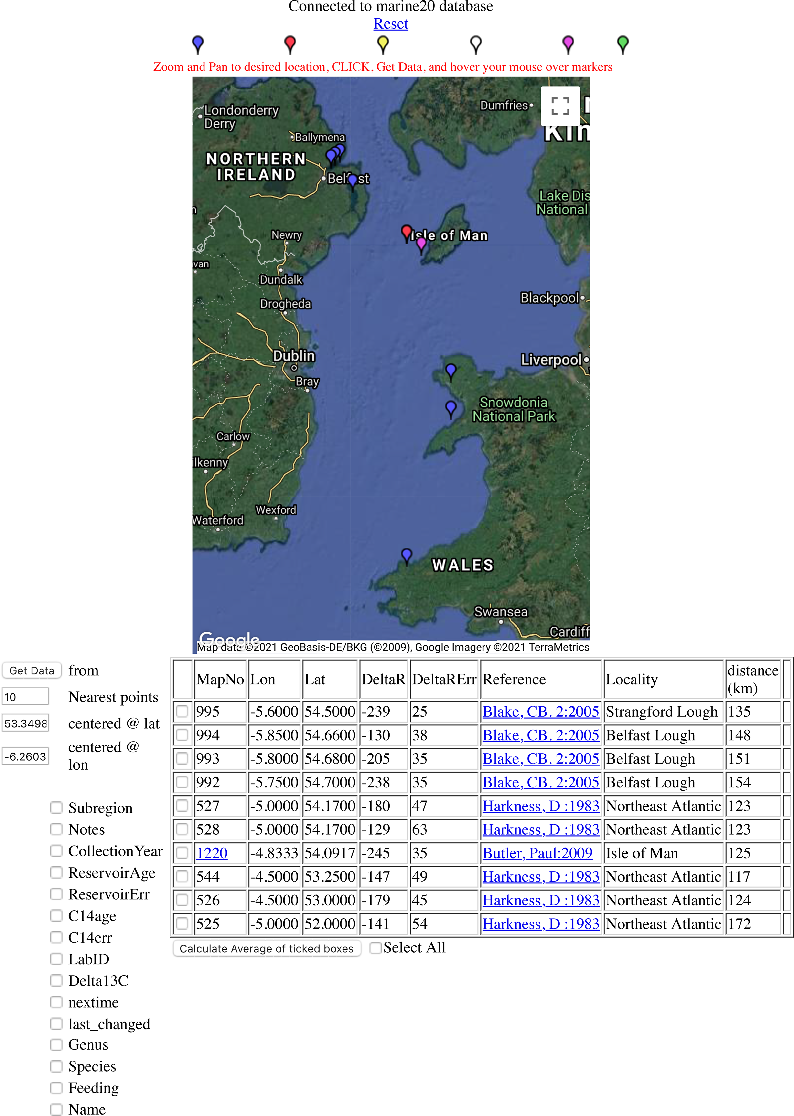
Figure 3 Location of 14C samples near Dublin taken from marine radiocarbon reservoir database (http://calib.org/marine/). Credit: Map data ©2021 GeoBasis-DE/BKG, Google Imagery ©2021 Terrametrics. Blue and red pushpins denote suspension and deposit feeding organisms, respectively, and purple are time histories rather than single determinations. Hovering over the different colored pushpins at the top of the webpage provides further definitions.
3.1.5 Are there situations where I should still use Marine13?
No, we do not recommend the continued use of Marine13. While we warned that Marine20 is not suitable for calibration in polar regions (Heaton et al. Reference Heaton, Köhler, Butzin, Bard, Reimer, Austin, Bronk-Ramsey, Grootes, Hughen, Kromer, Reimer, Adkins, Burke, Cook, Olsen and Skinner2020), this is not resolved (and is in fact made worse) by using an earlier marine calibration curve such as Marine13. Similar warnings were provided in the earlier calibration papers although less explicitly (e.g., Reimer et al. Reference Reimer, Bard, Bayliss, Beck, Blackwell, Bronk Ramsey, Buck, Cheng, Edwards, Friedrich, Grootes, Guilderson, Haflidason, Hajdas, Hatté, Heaton, Hoffmann, Hogg, Hughen, Kaiser, Kromer, Manning, Niu, Reimer, Richards, Scott, Southon, Staff, Turney and van der Plicht2013).
As described in Section 2.1.2, the issue in the polar regions is that during glacial periods, currently unknown local effects (e.g., changes in local sea-ice cover, strong winds, and altered ocean circulation) might have caused considerable localized, and short-term, changes in the surface ocean 14C depletion (Butzin et al. Reference Butzin, Köhler and Lohmann2017). These localized effects may have been distinct from those occurring on a global scale. Consequently, the assumption of an approximately constant ΔR(θ) cannot be justified in polar regions before the onset of the Holocene. This problem of additional localized, and short-term, variations in 14C depletion is not addressed by Marine13 or any of the earlier Marine calibration curves provided by the IntCal working group, and their use will not offer any improvements.
3.1.6 What should I do when calibrating marine 14C samples from polar regions?
Until our knowledge of past climate and models improve, and we can provide regional calibration curves, the calibration of marine 14C samples from polar regions, in particular during glacial periods, will remain a challenge.
Our cautious recommendation is that, if the sample is from the Holocene, one calibrate polar samples against Marine20 using a value of ΔR 20 which is also based upon 14C data from the Holocene. Ideally, one might estimate this ΔR 20 based on samples of similar calendar age to that which one is calibrating. This recommendation is made on the assumption that, during the Holocene, variations in sea-ice cover and high-latitude winds that might affect ΔR 20 should have remained small.
For polar 14C samples dating from before the Holocene, when ΔR(θ) may have varied significantly over time, great care must be taken in any calibration to prevent overconfidence in the calibrated date. Estimates of regional marine 14C depletion are available under fixed carbon cycle and climate scenarios using the three-dimensional LSG ocean general circulation model (Butzin et al. Reference Butzin, Heaton, Köhler and Lohmann2020) on PANGAEA (https://doi.pangaea.de/10.1594/PANGAEA.914500), however these scenarios are not transient in terms of climate. Hence calibrating against any individual scenario is still likely to lead to overconfidence.
The Marine20 group have proposed that a user calibrate polar samples against latitudinal-specific maximum-depletion and minimum-depletion curves separately and use two resultant ages to inform a bracketing which it is hoped encompasses the true calendar age (Heaton et al. Reference Heaton, Butzin, Bard, Bronk Ramsey, Hughen, Köhler and Reimer2022). These bracketing calendar age intervals are however wide—with differences of up to 1500 calendar years between the maximum- and minimum-depletion calibration scenarios. As more information becomes available on polar palaeoclimate and the extent of sea-ice, we expect calibration in these regions will become more precise.
3.2 Construction of the Marine20 Curve
3.2.1 Why did you choose the BICYCLE model to make Marine20 rather than other models?
The BICYCLE model (Köhler et al. Reference Köhler, Muscheler and Fischer2006) was chosen since it has sufficient complexity to accurately model the effect of a transient global-scale carbon cycle, yet remains sufficiently fast to be run hundreds of times and allow the uncertainty in the precise changes to the carbon cycle to be propagated though to Marine20.
For radiocarbon calibration, it is important not just to have a single best estimate for the calibration curve but to also understand the uncertainty around that curve. In the case of a model-based Marine calibration curve, uncertainty arises from two sources (Kennedy and O’Hagan Reference Kennedy and O’Hagan2001). Firstly, no computer model can perfectly represent the complexities of the Earth system. All models are simplifications and hence have a model discrepancy uncertainty. Secondly, the palaeoclimatic and carbon cycle changes we wish to feed into our ocean-atmosphere computer model are themselves somewhat uncertain. This uncertainty must be propagated through the model and introduces an input-related uncertainty to the Marine calibration curve.
Since carbon cycle models are complex and non-linear, we cannot reliably understand the input-related uncertainty by just running the model at the extremes of its climate and carbon cycle scenarios. Instead, we need to sample a range of scenarios from those that are potentially feasible and run each through the computer model. This creates an ensemble of possible Marine curves. We can then infer the input-related uncertainty using Monte-Carlo from the variability between the individual Marine curves in the ensemble. In the case of Marine20, we created 500 possible, BICYCLE-based, Marine curves for our ensemble by varying BICYCLE’s inputs according to our prior beliefs regarding their potential values.
While BICYCLE is a box-model, rather than a more complex Ocean General Circulation Model (OGCM), we believe it is sufficiently detailed to enable accurate modeling of large-scale MRA changes. We see little difference between the relative shapes of the BICYCLE-generated R 20 GlobalAv (θ) and the regional MRA estimates provided by the LSG OGCM (Butzin et al. Reference Butzin, Heaton, Köhler and Lohmann2020) as shown in Figure 2—see also Figure 4 in Heaton et al. (Reference Heaton, Köhler, Butzin, Bard, Reimer, Austin, Bronk-Ramsey, Grootes, Hughen, Kromer, Reimer, Adkins, Burke, Cook, Olsen and Skinner2020). This suggests that BICYCLE is able to capture most of the global-scale MRA temporal variations, and hopefully indicates that its model discrepancy uncertainty is small.
BICYCLE is also ideally suited to allow the Monte-Carlo approach required to understand the input-related uncertainty since it runs quickly. A more complex OGCM model, that could only be run very few times, would be of limited use for our Marine20 purposes. The use of BICYCLE allows Marine20 to provide good model representation yet still capture the significant input-related uncertainty which results from our lack of precise knowledge on the true palaeoclimate and carbon cycle inputs.
3.2.2 How did you choose the BICYCLE parameters?
The parameters in the BICYCLE model were not specifically tuned for Marine20. We took the same BICYCLE settings as had been used in a previous application of the model on 14C dynamics (Köhler et al. Reference Köhler, Muscheler and Fischer2006). A detailed description of the changing physical boundary conditions, based on palaeodata, that were prescribed for our implementation of BICYCLE can be found within Köhler et al. (Reference Köhler, Muscheler and Fischer2006)—specifically sea level, temperature, large scale ocean circulation, sea ice, and iron input which affects Southern Ocean marine biology. The parameters for BICYCLE were chosen to generate output that matched, as closely as possible, data-based reconstructions of changes in the carbon cycle during the past glacial cycle. This tuning focussed primarily on atmospheric CO2 concentration, but also considered the fit to δ 13C and Δ14C in the atmosphere. Further details can be found in Köhler et al. (Reference Köhler, Fischer, Munhoven and Zeebe2005).
For the creation of Marine20, the only three adjustments to the version of BICYCLE used in Köhler et al. (Reference Köhler, Muscheler and Fischer2006) were (i) a revised scheme for the implementation of carbonate compensation (i.e., the fluxes of carbonate ions between deep ocean and sediments); (ii) the external prescription of atmospheric CO2 concentration, as opposed to using the values BICYCLE internally generates. This violates mass conservation but brings the carbon cycle as close as possible to the observational data; and (iii) the external prescription of atmospheric Δ14C—individual posterior realisations of the IntCal20 curve were used, avoiding any assumptions on 14C production rates and enabling the propagation of uncertainty on atmospheric Δ14C levels through to the Marine20 curve. More detail on these adjustments are provided in Heaton et al. (Reference Heaton, Köhler, Butzin, Bard, Reimer, Austin, Bronk-Ramsey, Grootes, Hughen, Kromer, Reimer, Adkins, Burke, Cook, Olsen and Skinner2020). During previous studies using BICYCLE, oceanic information on carbon cycle changes were also used to evaluate model performance, e.g., the deglacial changes in the vertical gradient of δ 13C in the Southern Ocean (Hodell et al. Reference Hodell, Venz, Charles and Ninnemann2003).
The CO2 concentration record used to force the BICYCLE model for Marine20 was a spline through data from six Antarctic ice cores on their most recent age models (Law Dome, WAIS Divide, EPICA Dome C, EPICA Dronning Maud Land, Siple Dome, Talos Dome). All details on data selection and the spline calculation are contained in Köhler et al. (Reference Köhler, Nehrbass-Ahles, Schmitt, Stocker and Fischer2017).
4 QUESTIONS ON THE USE OF THE MARINE20 CURVE
4.1 Recalculating ΔR with the Marine20 curve
Whenever a new marine calibration curve is produced, a user will need to update the estimates of the additional regional components of MRA variation, i.e., the location specific ΔR(θ), before using the curve. We describe below how to do this using contemporary samples in the marine radiocarbon reservoir database hosted at http://calib.org/marine/ and with a user’s own 14C reference data. Typically, the samples in the reservoir database have calendar ages varying from ca. 200–0 cal yr BP. If a user has their own 14C samples from which to estimate ΔR, they can be of any calendar age.
As emphasized in Section 1.2.2, those users wishing to calibrate new 14C samples should ideally obtain estimates of ΔR in their location from samples of a similar calendar age to those they intend to calibrate—for example using paired terrestrial and oceanic samples, or samples for which an independent calendar date is available. However, we recognize this is often not possible and 14C data from the recent past is all that is available to estimate ΔR. In such cases, users should however give careful consideration as to whether, for the specific ocean location under study, an estimate of ΔR based on samples from the recent Holocene is suitable for calibration in much older time periods, and in particular the last glacial. This is especially relevant if the samples lie at higher latitudes, or within seas where ocean depth may have varied considerably. See Sections 2.1 and 4.2 for further discussion of these issues.
Users should also be aware that new samples are frequently added to the http://calib.org/marine/ radiocarbon reservoir database. As such new 14C data become available, estimates of ΔR 20 provided by the database may change. When calibrating, it is therefore important to note both the date of ΔR 20 calculation and the references used.
If no information is available on how a previous ΔR 13 was calculated, other than it was based on modern-day samples, we suggest a user can obtain an approximate ΔR 20 by subtracting 150 14C yrs (the approximate offset between the mean of Marine13 and Marine20 in the period from 200–0 cal yr BP) from the published value of ΔR 13, i.e., setting ΔR 20 = ΔR 13 − 150 14C yrs. To prevent the need for this approximation going forward, we recommend all authors provide sufficient detail on how their estimates of ΔR were created to ensure reproducibility for future calibration curve updates.
4.1.1 Recalculating a constant ΔR 20 based on data from the marine radiocarbon reservoir database
When we do not have detailed information on the changes in ΔR(θ) over time, if we want to calibrate new 14C samples we are required to make an approximation that it is constant, or at most slowly varying, for a given region. We can estimate this constant value ΔR 20 from the difference in 14C yrs of known age marine samples from that region and the Marine20 curve for that calendar age.
The ΔR values in the marine radiocarbon reservoir database at http://calib.org/marine/ (Reimer and Reimer Reference Reimer and Reimer2001) have been recalculated to provide a ΔR 20 for use with Marine20. We consider, as an example, estimating ΔR 20 in the ocean region off the coast of Dublin (53.35°N, 6.26°W). The locations of the 10 nearest marine 14C samples are shown in Figure 3. Some care should be taken when selecting which of the samples to use in estimating ΔR 20 for a given location. Samples from restricted sites, such as lagoons or fjords, may not be appropriate for more open ocean locations. Suspension feeding organisms usually provide a more accurate representation of the surface ocean age than deposit feeders. Migratory species may not have fed at the site where they were collected. The weighted mean and uncertainty of selected samples can be calculated for use in calibration. Note that the number of locations can be specified and additional information, such as collection year (given in AD/BC) and feeding type, can be requested from the menu at the left.
In Figure 4, we plot the Marine20 curve and the ten 14C observations identified in the map of Figure 3 which have been selected from the marine radiocarbon reservoir database. We calculate the offset between the curve and the samples in the calendar year of each 14C sample. These provide estimates of ΔR 20(θ) and may be used to give some indication of how reliable an assumption that it remains approximately constant over time is.
In the case we wish to approximate ΔR 20(θ) as constant, e.g., to allow calibration of unknown age samples, then these values can be suitably averaged. In this case we get an estimate for ΔR 20 of −201 ± 46 14C yrs (1σ). These calculations are all performed online within the marine radiocarbon reservoir database.
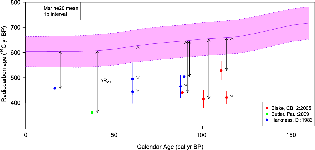
Figure 4 Known-age marine 14C samples in the region off the coast of Dublin compared to the Marine20 calibration curve (shown in pink). We plot the 1σ-intervals on the 14C observations and the Marine20 curve. The offsets, highlighted as arrows, form our estimate for ΔR 20(θ) which we are typically required to assume as approximately constant to calibrate new, unknown age, marine 14C samples from the region. (Please see online version for color figures.)
4.1.2 Recalculating a constant ΔR 20 based on own reference 14C samples
If a user has their own 14C dated samples they can calculate a ΔR 20 using the link to the deltar software (Reimer and Reimer Reference Reimer and Reimer2017). These samples can be of known collection ages; independently dated ages, such as via U-Th or optically stimulated luminescence (OSL) dating; or contemporaneous marine and terrestrial radiocarbon ages including radiocarbon dated tephra deposits. The software will provide the 68% (1σ) and 95% (2σ) confidence intervals for ΔR 20. Most calibration programs expect a 68% (1σ) uncertainty on ΔR.
4.2 What Should a User Do if They Think ΔR has Changed Significantly from the Present-Day Values?
The assumption that modern-day 14C samples are representative of ΔR(θ) at times a long way further back in the past, i.e., a constant ΔR, should rightly be treated with caution. It is only proposed in situations where no more detailed information on changes in ΔR(θ) is available. If such data is available, we recommend calculation of a ΔR 20 using 14C samples of a similar calendar age to those that one wishes to calibrate. Using such contemporaneous samples should provide an improved estimate of ΔR 20 for the time period of the sample you wish to calibrate.
If a user is calibrating a 14C sample for which they believe that there may be additional variation in ΔR(θ), but does not have contemporaneous reference data on which to estimate the relevant value, they may wish to add an additional uncertainty to the present-day ΔR 20 estimate before calibration.
4.3 How should a user treat the MRA from the Southern Hemisphere?
Our definition of MRA, given in Section 1.1, considers the offset in radiocarbon years (14C yrs) between the surface-layer dissolved inorganic carbon and the contemporaneous Northern Hemispheric atmosphere (Reimer et al. Reference Reimer, Austin, Bard, Bayliss, Blackwell, Ramsey, Butzin, Cheng, Edwards, Friedrich, Grootes, Guilderson, Hajdas, Heaton, Hogg, Hughen, Kromer, Manning, Muscheler, Palmer, Pearson, van der Plicht, Reimer, Richards, Scott, Southon, Turney, Wacker, Adolphi, Büntgen, Capano, Fahrni, Fogtmann-Schulz, Friedrich, Köhler, Kudsk, Miyake, Olsen, Reinig, Sakamoto, Sookdeo and Talamo2020). The Southern Hemispheric (SH) atmospheric 14C level is somewhat offset, and depleted, compared to the Northern Hemispheric levels, with the SH atmosphere being 36 ± 27 14C yrs older (Hogg et al. Reference Hogg, Heaton, Hua, Palmer, Turney, Southon, Bayliss, Blackwell, Boswijk, Bronk Ramsey, Pearson, Petchey, Reimer, Reimer and Wacker2020). This atmospheric offset changes over time and is known as the interhemispheric 14C gradient.
If we are interested in assessing the level of 14C disequilibrium between the surface-layer of site in the SH oceans and the SH atmosphere with which those sites directly interact, we must therefore be somewhat careful. By calculating the overall MRA at an ocean site with respect to the NH atmosphere, we will obtain MRAs at SH ocean sites that provide overestimates for the actual level of 14C disequilibrium from the SH atmosphere. The size of this overestimate will be the value of the NH-SH atmospheric offset. Since Marine20 is created by forcing the BICYCLE model with the NH atmospheric, our estimates of ΔR 20(θ) at SH ocean sites will also include a component caused by the NH-SH atmospheric offset rather than ocean changes.
When calibrating marine 14C samples from the SH, one can still use the Marine20 curve so long as you estimate a ΔR 20(θ) for the site. The effect of forcing Marine20 by the NH atmospheric 14C levels, rather than the SH, should be compensated for through estimation of ΔR 20(θ). This is not however the case if the MRA correction is based on, e.g., paired atmospheric-marine samples for the SH site.
We also note that there are hints that the interhemispheric 14C gradient has varied in the past, notably due to winds and ocean changes (e.g., Rodgers et al. Reference Rodgers, Mikaloff-Fletcher, Bianchi, Beaulieu, Galbraith, Gnanadesikan, Hogg, Iudicone, Lintner, Naegler, Reimer, Sarmiento and Slater2011; Capano et al. Reference Capano, Miramont, Shindo, Guibal, Marschal, Kromer, Tuna and Bard2020). Hence, while those studying sites in the SH can still use the Marine20 curve since the interhemispheric offset is relatively small, more work is needed in the future to better constrain and reduce the uncertainties associated with the calibration of 14C ages on marine samples.
5 ADDITIONAL QUESTIONS
5.1.1 Can I just calibrate my 14C samples against the atmospheric IntCal20 curve directly using an estimate of the overall MRA R Location (θ) for my region that I obtained from a particular calendar year (e.g., by looking at the offset to IntCal20 at 0 cal yr BP)?
No, using the atmospheric IntCal curves on 14C samples from the open ocean directly isn’t a reliable calibration approach and will result in incorrect calendar age estimate. One should always calibrate open ocean marine 14C data against the Marine calibration curves using a regional ΔR adjustment rather than against an atmospheric calibration curve. The only exception to this is the case of 14C samples from semi-closed basins, closed lakes and small seas, which we discuss in Section 5.1.3.
The marine (radiocarbon age vs. calendar age) 14C calibration curve is not only offset from the atmospheric 14C curve. As explained in Section 2, it is also much smoother as the ocean removes much of the high-frequency variation seen in the atmospheric 14C signal and wiggles are somewhat delayed. Since the ocean responds more slowly to changes in 14C production rates compared to the atmosphere, the overall MRA R Location (θ) fluctuates very rapidly—such fluctuations in overall MRA occur when the atmospheric 14C level has already changed but the ocean is still in the process of responding. This high-frequency variability in overall MRA can be clearly seen in the estimate of R 20 GlobalAv (θ), the global-scale temporal variations, plotted in Figure 1a. The necessary smoothing of the radiocarbon age vs. calendar age 14C oscillations seen in the open ocean cannot be obtained with a constant overall MRA R Location (θ). Such a constant R Location (θ) would simply shift the atmospheric radiocarbon age vs. calendar age calibration curve but leave all the oscillations the same.
A user can estimate the total MRA, R Location (θ), in a single calendar year by looking at the offset between IntCal20 and a specific 14C sample. However, there is no guarantee that this single year estimate of total MRA will be representative of the total MRA for other calendar years due to this inherent smoothing of the atmospheric radiocarbon age vs. calendar age 14C variations that occurs in the oceans. Such a user cannot therefore use their single-year point estimate of R Location (θ) to calibrate new samples, of different calendar ages, against the atmospheric IntCal20 curve.
Marine20 models the damping present in the ocean during its construction, factoring out the high-frequency MRA changes in the resultant curve through its estimate of R 20 GlobalAv (θ). Figure 1a shows this R 20 GlobalAv (θ) during the Holocene. Most of the rapid variation shown here is a result of the smoothing, and delay, of the atmospheric IntCal20 14C signal that occurs in the ocean. Since, when using the Marine20 curve, the atmospheric damping has been factored out through the highly variable R 20 GlobalAv (θ), a user only needs to consider the additional local effects ΔR(θ). These are less likely to relate to damping and so should hopefully remain more constant.
Further, there are physical reasons why changes in atmospheric CO2, 14C production and carbon cycle will significantly affect the MRA before the onset of the Holocene, typically increasing the level of oceanic 14C depletion compared with the levels seen—again, see Figure 7 of Heaton et al. (Reference Heaton, Köhler, Butzin, Bard, Reimer, Austin, Bronk-Ramsey, Grootes, Hughen, Kromer, Reimer, Adkins, Burke, Cook, Olsen and Skinner2020). If one calibrates against Marine20 these effects are included. However, they are not if one simply applies a constant offset to the IntCal20 curve.
Finally, the use of MRA estimates based on previous iterations of Marine and IntCal curves will lead to incorrect inference. Each set of curve updates require the recalculation of MRA estimates.
5.1.2 How can a user get reference marine 14C data from glacial periods to estimate a ΔR 20(θ)?
The Marine20 curve includes the global-scale changes in the MRA for glacial periods as discussed above. In most non-polar regions, we suggest this can be used together with an estimate of ΔR 20 based upon independent marine 14C from the recent past. Otherwise, it is very difficult unless you have paired marine/terrestrial 14C dated material (see e.g., Petchey and Schmid Reference Petchey and Schmid2020); a known-age tephra layer (Sikes et al. Reference Sikes, Samson, Guilderson and Howard2000; Siani et al. Reference Siani, Paterne, Michel, Sulpizio, Sbrana, Arnold and Haddad2001); or a sample dated in some other way such as via U-Th or OSL (e.g., Toth et al. Reference Toth, Aronson, Cheng and Edwards2015, Reference Toth, Cheng, Edwards, Ashe and Richey2017; Hirabayashi et al. Reference Hirabayashi, Yokoyama, Suzuki, Esat, Miyairi, Aze, Siringan and Maeda2019; Hua et al. Reference Hua, Ulm, Yu, Clark, Nothdurft, Leonard, Pandolfi, Jacobsen and Zhao2020). Note that while some of these references relate to data from the Holocene, the methods they desribe could also be applied to older samples. Stratigraphic alignment of cores to terrestrial records may also provide a method to estimate ΔR 20(θ) and MRA (e.g., Muschitiello et al. Reference Muschitiello, D’Andrea, Schmittner, Heaton, Balascio, deRoberts, Caffee, Woodruff, Welten, Skinner, Simon and Dokken2019; Skinner et al. Reference Skinner, Muschitiello and Scrivner2019; Waelbroeck et al. Reference Waelbroeck, Lougheed, Vazquez Riveiros, Missiaen, Pedro, Dokken, Hajdas, Wacker, Abbott and Dumoulin2019; Brendryen et al. Reference Brendryen, Haflidason, Yokoyama, Haaga and Hannisdal2020).
5.1.3 How can I calibrate 14C samples from closed seas and large lakes?
None of the Marine calibration curves are intended for closed seas and lakes. Closed seas and lakes have their own carbon turnover and reservoir offset that is independent of ocean circulation. Further complications arise, especially for lakes, since the 14C offset between the surface water and the atmosphere is often affected by both the release of old (but not necessarily dead) organic carbon from soils and peats; and dead inorganic carbon (a hard water effect) entering the lake from its inflows/groundwater. The sensitivity to external inputs also depends on the lake’s dissolved inorganic carbon which can vary widely, as well as the salinity from freshwater to hypersaline lakes. These are both fundamentally different from an open ocean reservoir age linked to 14C decay during transport in a large water body and to limitations in the air-sea gas exchange.
Consequently, for the calibration of such samples, none of the Marine calibration curves are appropriate—they are based on open-ocean estimates of R GlobalAv (θ) that include a large, 14C-deficient, deep ocean reservoir. However, atmospheric IntCal calibration curves are also unlikely to be entirely appropriate for closed seas and large lakes since the carbon turnover will still smooth away at least some of the high-frequency (radiocarbon vs. calendar age) atmospheric variation. In reality, the damping with closed seas and large lakes is likely to lie somewhat between that seen in the (heavily damped) open-ocean Marine calibration curve and the (undamped) atmospheric calibration curve.
It is unfortunately not possible to give an off-the-shelf universal solution for those wishing to calibrate 14C samples from non-open waters. We therefore defer to the user to decide upon, and justify, an appropriate approach to calibration based upon their expert knowledge of the specific sea or lake. For large lakes and closed seas, hydrological modeling to determine the surface water 14C depletion (using models without deep water compartments) may be most appropriate (e.g., Yu et al. Reference Yu, Shen and Colman2007). For smaller lakes, where there are known age shells or other lacustrine organisms available, then the simplest approach would be to measure the 14C ages of these samples and calculate the lake’s offset to the atmospheric IntCal20 curve, with an estimated fossil fuel correction for post-industrial age samples. This atmospheric offset can then be used to calibrate other 14C samples directly against the IntCal20 curve. This suggestion comes with considerable caveats however, since the 14C reservoir offset in a lake can vary over time for many reasons including changing hydrological cycles. Paired terrestrial and lacustrine or sediment samples may therefore be needed throughout the core to determine the appropriate atmospheric 14C offset to apply.
In the case of semi-closed basins (i.e., those which have sometimes been cut-off partially or completely from the open ocean, but at other times have not) a 14C user must consider both the present open-ocean exchange and the time evolution of these exchanges due to past sea level changes. Complications will inevitably arise, ranging from basins that were completely disconnected during the LGM and Late Glacial (e.g., Baltic Sea, Black Sea) to basins in which hydrology was probably affected in a more subtle way (e.g., Mediterranean Sea, Red Sea, and Arctic Ocean with the closure of the Bering Strait). Again more research is needed to understand the evolution of reservoir ages in such semi-closed basins (e.g., of the Black Sea Soulet et al. Reference Soulet, Ménot, Garreta, Rostek, Zaragosi, Lericolais and Bard2011).
5.1.4 What should be done for 14C samples that arise from different water masses such as the deep and intermediate ocean?
It is important to also stress that Marine20, and all previous marine calibration curves, are only useful for marine samples which grew at the ocean surface. As a community we are a great distance from being able to provide individual marine calibration curves for the deep and intermediate layers in the main ocean basins. Such work will require much more understanding of ocean circulation. Currently, deep sea corals and benthic foraminifera can provide data from different water masses.
5.1.5 How can a user propose 14C data for inclusion in the marine reservoir database?
Researchers with either known age or independently dated pre-bomb 14C measurements, which can be used to calculate ΔR 20, are encouraged to send published papers and relevant information to R. or P.J. Reimer for inclusion in the database. Please note however that, because of its setup, which assumes a known-age or independently dated sample with insignificant calendar age uncertainty, paired marine and terrestrial data cannot be included in the current radiocarbon reservoir database. The user can of course still calculate ΔR 20 values for their own paired samples using the deltar software provided through the database.
5.1.6 What information should 14C users include in their papers to ensure adherence to open science best practices?
Since all 14C calibration curves are regularly updated, it is essential to ensure that calibration is reproducible, and critically that all calendar dates and inference can be revised, for future calibration curve updates. All 14C users should therefore provide the conventional radiocarbon ages for their samples (in 14C yr BP) and the accompanying lab codes. They should also clarify which calibration curve they have used for the reader as advised by Millard (Reference Millard2014).
When linking and referencing research, users should also ensure that they are not comparing calendar dates, or inference, that have been obtained with different versions/updates of calibration curves. For example, it is not reliable to compare inference and calendar dates across papers which have been inconsistently calibrated, with some calendar age estimates being provided by calibration against IntCal/Marine09 while others have been estimated using IntCal/Marine13 and/or IntCal/Marine20.
In the case of the Marine calibration curves, this consistency is also important if estimating changes in ΔR 20(θ) by looking at the offset against Marine20. One must not mix estimates of ΔR 20(θ) with previous estimates of ΔR 09(θ) or ΔR 13(θ) that were obtained by looking at the offset to Marine09 or Marine13. This is particularly the case when studying changes in the last glacial period since Marine09 and Marine13 incorporated no global-scale carbon cycle changes (see Figure 2 and Section 3).
Authors are also encouraged to ensure that the method they used to estimate ΔR 20 for calibration is entirely reproducible for future Marine calibration curve updates. This will require an explanation of the method used and referencing of the original publications in the marine database that have been used to determine ΔR 20.
5.1.7 Do all editors of all journals know that they have to check that the date of the marine database used has to be mentioned in the bibliographic reference, since it is continuously updated?
No, reviewers and editors will need to be encouraged to check that ΔR 20 values have been used, either because the subscript is included or the date when the database was used is given.
ACKNOWLEDGMENTS
P. Köhler and M. Butzin are supported by the German Federal Ministry of Education and Research (BMBF), as Research for Sustainability initiative (FONA); www.fona.de through the PalMod project (grant numbers: 01LP1505B, 01LP1919A), which also covered the Open Access fees. E. Bard is funded by EQUIPEX ASTER-CEREGE and ANR MARCARA.


 Open access