EXPERIMENTAL

Figure 1 shows our interface for CF hyphenation of an elemental analyzer (EA) model Vario MICRO (Elementar, Germany) with the ion source of a MICADAS AMS (Szidat et al. Reference Szidat, Salazar, Vogel, Battaglia, Wacker, Synal and Türler2014). In the “CN” mode, the EA combusts the sample and releases the peaks corresponding to N₂, CO₂ and other gases in sequence by thermal desorption using helium as gas carrier at 135 cm³/min. The peaks are detected with a thermal conductivity detector (TCD). The EA is connected to the gas interface through a 1/16” stainless steel tubing (inner diameter = 0.75 mm, length = 5 m). Figure 1b shows our modified “CN” method which releases the CO₂ at warmer temperature than normal conditions in order to create a sharp peak. The pressure at the head valve of the helium bottle is lower than normal conditions (1.2 bar relative to ambient pressure). In the beginning of the run, the split valve is closed and all the flow enters the dead volume (flexible bellow tube size: L = 30 cm, 50 cm³), exiting to the vent through the purge valve while a small fraction still reaches the ion source, keeping the lines flushed. The flow is controlled by a mass flow controller (MFC) model MCW500 (Alicat, USA) and by a restriction tube at point “1” (1/16” tubing, i.d. = 0.1 mm, L = 80 mm). The MFC is set to a medium flow of 75 cm³/min at 150 s to guarantee the CO₂ residence time inside the dead-volume to be long enough (60 s). This residence time can be measured with a non-dispersive infrared (NDIR) detector tuned for CO₂ (Sunset Laboratory, USA) which can be mounted before or after the dead volume as indicated by the points “1” and “2” of Figure 1a. After 210 s, the MICADAS data acquisition is started and at ∼270 s, the control program searches for the CO₂ peak height from the recorded TCD signal. The end time (t_end = 300 s) is the end of the loading protocol, when the CO₂ peak is almost at the end of the dead volume. At t_end, the purge valve is closed and the split valve is opened. This new arrangement directs some of the carrier flow to the split vent at a rate controlled by the needle valve, keeping the dead volume pressurized around a desired value. This pressurization assures that an overpressure is maintained at the splitting “Tee” and the CO₂ does not flush back into the split vent. At t_end, the MFC is set to deliver a flow into the ion source of 1–5 cm³/min depending on the capillary i.d. and the pressure of the dead volume. All the steps before t_end belong to the CO₂ loading into the dead volume while all the later steps regard to the ion source injection protocol. t_end defines t = 0 for Figures 3–4 (see below).

Figure 1 Scheme of the experimental method. (a) Experimental set up with a green trace line indicating the CO₂ loading path, (b) Elemental analyzer conditions during CO₂ loading. At t_end, the pneumatic valves split the inflow, (c) Picture of the dead volume. (Please see electronic version for color figures.)

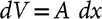
Figure 2 Illustration of the mathematical model during the high flow (75 cm³/min) loading. (a) Scheme of the dead volume with a CO₂ peak that starts at the entrance and then diffuses and drifts during 20 s, (b) Calculations of the CO₂ concentration showing how the peak drifts at several time steps. Wall reflection at the exit is highlighted with a red circle, (c) Calculation of the CO₂ concentration at the exit of the dead volume as a function of time (C[L,t]) compared to the measured signal of a NDIR detector.

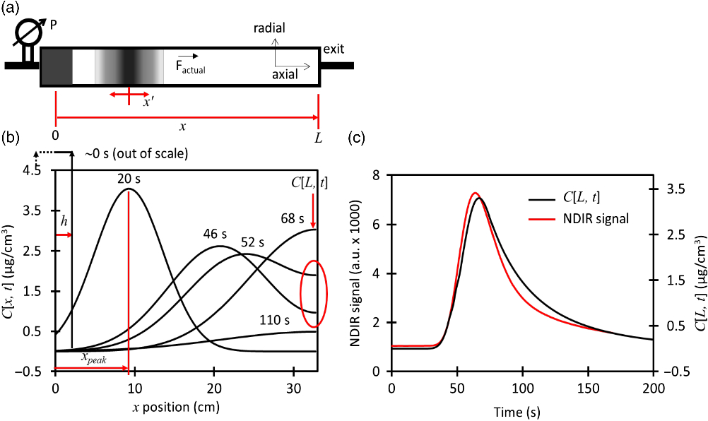
Figure 3 Time evolution and quality parameters of ionization using the whole protocol (CO₂ loading and injection) for the dead-volume CF interface with a capillary i.d. of 0.18 mm. (a) Ion current signal, (b) Ionization yield, (c) Overlap of calculated CO₂ concentration, mass flow and ion current for 70 µg C normalized to these conditions:C[L,t] = 1.1 µg C/mL, ¹²C^– = 3.3 µA and $\˙ m$ = 3.5 µg C/min.

Figure 4 Summary of the empirical and calculated data for 3 different injection capillaries as a function of the injected mass. (a) maximum ion current, (b) average ionization efficiency, (c) calculated CO₂ concentration, and (d) calculated mass flow. The arrows indicate the onset of ionization suppression.

The control program of the interface is written in Visual Basic 2017 (community edition). It commands all the valves, involved devices and their respective software in real-time. The program controls the MICADAS and the EA by TCP commands. Both valves are shut-off valves with pneumatic actuation. Without pneumatic pressure, the split valve is in the open state and the purge valve is in the close state. In this way, both valves can share a single pneumatic feed. The pneumatic feed is delivered by a single valve DVI 205M (Pfeiffer, USA) connected to a home-made power relay which is controlled by a small signal from an ARDUINO board model MEGA 2560 (Arduino, Italy). The MFC hardware comes with the option for serial communication and control. The R program (R Core Team 2013) was employed to develop the algorithm and mathematical models. Later, those algorithms were implemented in a Visual Basic program, so it could track and display the calculated mass flow in real time. This method enables the system to be simple and low-cost but also it is able to carry out the loading and injection protocols automatically.

Aliquots of D-(+)-sucrose (Sigma Aldrich, USA) standard solution at 10 µg C/µL in ultra-pure water (18 MΩ·cm, TOC < 2ppb) are deposited in aluminum caps (Elementar, Germany) which are closed and set in the EA autosampler. The standards are solid crystals of sodium acetate (fossil; p.a., Merck, Germany), C5, C6 and C7 from IAEA and Oxalic Acid II (Oxa II) from NIST (SRM 4990c). The MICADAS is operated at 135ºC Cs temperature, 128 W power for the Cs reservoir heater and at a background pressure in the ionizer chamber of 2 × 10^–6 mbar during gas injection.

RESULTS AND DISCUSSION

Mathematical Model

We developed an algorithm that tracks the CO₂ peak along the dead volume and calculates the carbon mass flow at the exit or position L. The model is illustrated in Figure 2 and described in detail in the supplemental materials.

The CO₂ peak with mass (m) starts as a disk with half width (h) and cross section area (A) determined by the container’s inner diameter. The initial CO₂ concentration (C ₀ ) is uniform in the axial and radial directions as defined by Equation (2). The axial speed is calculated, during the loading

$${C_0}\; = {\rm{ }}m/\left( {2hA} \right)$$ (2)

and injection protocols, from the measured standard flow corrected by the pressure and the cross section area of the dead volume. The CO₂ drift (x _peak ) is illustrated in Figure 2a and 2b in which the center of the peak is moved until certain axial position at the same speed of the carrier gas during a small amount of time (dt = 1 s) each time.

$$C\left[ {x',t} \right] = {1 \over 2}{C_0}\left[ t \right]\mathop \sum \limits_{n = - 1}^1 \left\{ {erf\left( {{{h + 2nL - x'} \over {2\sqrt {Dt} }}} \right) + erf\left( {{{h - 2nL + x'} \over {2\sqrt {Dt} }}} \right)} \right\};t > 0$$ (3)

The concentration profile along the whole axial coordinate is broadened using Equation (3) which is based on the error function (erf) and takes in account initial width, time (t), Diffusivity (D), axial position and gas reflection when encountering a wall at a distance (L) (Crank Reference Crank1975). We use a pressure-dependent diffusivity as determined for helium-CO₂ mixtures by (Bogatyrev and Nezovitina Reference Bogatyrev and Nezovitina2012) at 25°C. The concentration profile relative to the axial direction is calculated with a travelling coordinate x’, where x’ = 0 at the peak center located at x _peak position. The coordinates are transformed by Equation (4). Wall or boundary reflection is useful to realistically simulate the moment

$$x' = {\rm{ }}x{\rm{ }}-{\rm{ }}{x_{peak}}$$ (4)

when the peak reaches the end of the dead volume located at position L and is impeded to enter the injecting capillary. We observed that the series n = –1 to 1 was enough to approximate our results, although it should be noted that the original form of Equation (3) is an infinite series with n = –∞ to +∞ (Crank Reference Crank1975). We assume that diffusion, wall reflection and mass loss are the only factors that change the concentration profile in the axial direction. The concentration profile in the radial direction is kept uniform during the whole simulation. In this work, the ratio of dead volume length to disk initial width h is ∼12 and the length to inner diameter ratio is ∼12. Our assumptions will not work for neither small L/h nor L/i.d. ratios where there is gas mixing instead of lateral diffusion. Figure 2b illustrates how the concentration profile changes in time and in axial position. The red circle highlights how the wall reflection affects the CO₂ concentration peak tail at the exit of the dead volume (C[L,t]). Equation (5) gives the real-time mass flow as the product of the instantaneous CO₂ concentration in µg C/cm³ with the carrier flow in cm³/min as explained in Equation (1).

$$˙ m = C[L,t]\;˙ V$$ (5)

The mass inside the dead volume is calculated by numerical integration of Equation (3) with respect to volume for the whole range x = –h to L. The integration volume element is converted into axial units using $dV = {\it{A}}\,\,dx$ . The mass loss is the product of the mass flow delivered into the capillary during the interval dt. Then, C ₀ is corrected to account for mass loss, the peak is let to drift again during dt and the algorithm is repeated. When the CO₂ peak reaches the end position, the drift value is kept constant at x _peak = L but time t continues increasing. The theory can be tested at high flow by carrying out the CO₂ loading protocol without splitting the flow, letting the CO₂ escape through the purge valve and including a non-dispersive infrared (NDIR) detector connected to the purge vent at position “2”. The dynamic response of this detector is linear for all the range of concentrations used in this work. The medium flow is kept constant at 75 cm³/min until the whole peak is detected. The theory is not tested for the injection protocol because of the lack of sensitivity of the NDIR detector at low flows. Figure 2c shows a very good agreement between the shape of the calculated CO₂ concentration C[L,t] at the exit of the dead volume with the NDIR signal. We are not able to calibrate the NDIR signal to instantaneous concentrations, thus we cannot prove the accuracy of the model. Nevertheless, the calculated C[L,t] value seems to be reliable.

Empirical Results

Figure 3a shows how the ¹²C^– current signal changes during continuous-flow (CF) injection with the dead-volume interface coupled to the EA. A maximum current of 14.4 µA is reached during the time evolution of the 50 µg C injection. The maximum current for 50 µg C is the highest within the group of masses evaluated. Higher masses like 70 µg C produce the curve “4” in which the current starts to increase but suffers a sudden drop at 120 s that lasts until ∼800 s where the signal starts to recover again. This behavior reflects the ionization suppression which has been observed before for CF injection into AMS ion sources (Agrios et al. Reference Agrios, Salazar and Szidat2017). Equation (6) is used to calculate the instantaneous ionization efficiency at the low-energy side of the AMS where I is the ion current signal (µC/s), F is Faraday’s constant (96485 C/mol), $˙ m$ is the instantaneous mass flow (µg C/s) and M _C is molar mass of carbon (12.011 g/mol). The ion current is recorded continuously and is only limited by the recording frequency of the detector (0.1 Hz). Hence, it is possible to calculate an “instantaneous” mass flow and ionization yield at any given moment. Figure 3b shows the ionization yield for the same group of

$$Eff.{\rm{}}\left( {\rm{\% }} \right) = {{I{\rm{}}} \over {˙ m{\rm{}}}}{{{M_c}{\rm{}}} \over {{\rm{}}F}}{\rm{}} \cdot 100{\rm{\% }}$$ (6)

injected masses as Figure 3a. The yield for 50 µg C reaches higher values than lower masses and the strong ionization suppression for 70 µg C is reflected in its reduction in ionization yield. The general behavior of the current and ionization yield are illustrated in Figure 3b and 3c for 70 µg C. In the beginning of the injection (< 50 s), the MFC flow reading is very low; however, the actual flow going into the ion source is higher. Momentarily, the actual flow is driven by the dead volume pressure due to the position of the MFC. This causes an underestimation of the mass flow ( $˙ m$ ) that lasts until the system equilibrates at ∼50 s. As consequence, the actual $˙ m$ creates a small current (I) that in comparison with the underestimated $˙ m$ translates into an artificial ionization yield peak as indicated with an arrow. After 100 s, the ion current is triggered when the mass flow is around 1 µg C/min. The onset of the current suppression and its recovering points occur when $˙ m$ is ∼2.0 µg C/min as indicated by the arrows. In this case, $˙ m$ reaches a maximum of 3.5 µg C/min. This suggests that the ionization suppression is reversible and only appears when the instantaneous $˙ m$ is higher than an onset value. The mass flow never reaches the suppression onset for relatively low masses (20–50 µg C), so their current signals are not affected. It should further be noted that the CO₂ concentrationC[L,t] starts to rapidly increase earlier than $˙ m$ . This is because, in the beginning of injection, the front of the CO₂ peak is located at the end of the dead volume (L), hence C[L,t] is already increasing. However, the carrier flow is very low (1.3 cm³/mL), thus the estimated $˙ m$ is also low at this moment. Later, the carrier flow slowly increases, reaching 3.2 cm³/mL at 600 s and after a quick increment, it reaches 5 cm³/mL at 900 s. The same flow increment pattern is used for all measurements with the exception of Table 1 and this pattern is intended to keep the dead volume pressure relatively constant. The maximum value of C[L,t] and $˙ m$ time plots change proportionally with the mass, but they all have the same shape and width (see example in Figure 3c).

Table 1 Radiocarbon analysis of grains of standard materials showing the St. dev. as the standard deviation of the repeated measurement (n = 2), uncertainty as the average counting statistics uncertainty at 1-σ level and accuracy as the relative difference to the nominal value.

The long increasing tails of the ionization yield starting at 750 s occur when the CO₂ concentration is decreasing but the carrier flow is increasing rapidly. $˙ m$ is the product ofC[L,t] and flow, consequently, $˙ m$ decays slowly. The ion current tail is not following the fast decay of the CO₂ concentration, but it is variating more with the long tail of $˙ m$ . However, the variation of the ion current is not perfectly governed by $˙ m$ . Our model estimation is based on perfect cylindrical tubing, but the dead volume has irregular geometry and can suffer of turbulent flows due to the considerable volume of the pressure gauge and the irregular shape of the dead volume walls as shown in Figure 1. The CO₂ that is trapped in the turbulent flow and irregular geometries is released at a later time, increasing even more the tail of the ion current signal. These non-ideal situation creates inaccuracies in our mathematical model.

Figure 4 summarizes the data presented in Figure 3 for three different capillary sizes. Similar as in Figure 3, ionization suppression is observed for all capillaries, when the instantaneous $˙ m$ reaches the onset value. Figures 4a and 4b show how the maximum current and average ionization efficiency increase with the mass until reaching a maximum from where the signals start to be suppressed. The average ionization efficiency is defined as the average instantaneous ionization efficiency for the time range of 50–750 s. All capillaries reach similar levels of maximum current, however, the biggest capillary (0.18 mm) can reach higher efficiencies. On the other hand, the mass working-range for the largest capillary is comparatively narrow. This means that it is better to use large capillaries for small masses. The mass range can be extended by using lower carrier flows during injection of high masses because this avoids the mass flow to reach the suppression onset as it is done for Table 1. In the other hand, high carrier flows should be used for lower masses. Figure 4c indicates that the ionization suppression starts at different CO₂ concentrations and the CO₂ concentration at the onset is very different for each capillary. On the contrary, Figure 4d shows that the onset of ionization suppression falls in a narrow range (2.0–2.3 µg C/min) for all capillaries. This reflects that the signal for this type of interface and ion source is not controlled by the CO₂ concentration alone, but by the mass flow.

Preliminary results are shown in Table 1 using the whole automatized protocol, but quantifying the CO₂ using the height of the EA peak and limiting the maximum mass flow to 2.0 µg C/min by decreasing the carrier volumetric flow setting on real time. For this range of masses, the typical precision for non-CF interfaces using Oxa II is ca. 0.6–0.8% (Hoffmann et al. Reference Hoffmann, Friedrich, Kromer and Fahrni2017; Tuna et al. Reference Tuna, Fagault, Bonvalot, Capano and Bard2018). Although the results are comparable with non-CF works, Table 1 just represents a proof-of-concept due to the small number of repetitions. Further statistical characterization including constant and cross contamination shall be carried out in future.

In general, our CF interface gives 4–6% optimum ionization yields which are lower than the optimum yields reported for non-CF interfaces. We should mention that our Cs vaporization temperature (135°C) is much lower than for other studies. Hoffmann et al. (Reference Hoffmann, Friedrich, Kromer and Fahrni2017) used 160°C to achieve 4–6% yields. Fahrni et al. (Reference Fahrni, Wacker, Synal and Szidat2013) obtained a 6% yield at 150°C. Nevertheless, we think that at similar source conditions non-CF interfaces should be just slightly more efficient, because they work at nearly steady-state conditions and at low carrier flows (<1.4 cm³/min). In contrast, for our CF interface, the carrier flow is much higher and the carbon mass flow is continuously changing. Our data suggests that the higher carrier flow range (1–5 cm³/min) has small detrimental impact on the ionization yield comparing with non-CF yields. High carrier flows increase the background gas, interfering with the Cs⁺ beam; but perhaps at the same time, this cools down the Ti surface which increases the CO₂ absorption. The optimal carbon mass flows from previous studies (Fahrni et al. Reference Fahrni, Wacker, Synal and Szidat2013; Hoffmann et al. Reference Hoffmann, Friedrich, Kromer and Fahrni2017) and from our results are in the same range; the ionization mechanism is therefore more governed by the amount of CO₂ that is fed onto the Ti surface per unit time (independently of the type of injection flow or capillary size), if the Cs⁺ beam density is kept constant.