


1. INTRODUCTION
This paper presents a method for creating OxCal Bayesian models without going through the complex process of writing OxCal code. Our approach uses the recently published ChronoLog software (chrono.ulb.be; Levy et al. Reference Levy, Geeraerts, Pluquet, Piasetzky and Fantalkin2021) as a graphical user interface (GUI) to generate OxCal scripts. It enables users with no training in programming or mathematics to easily build Bayesian models, even intricate ones, with the help of a user-friendly interface. The generated scripts can include termini post and ante quem, duration bounds, and several types of synchronisms. To the best of our knowledge, no GUI currently exists that automatically creates Bayesian OxCal models. In 2015, in a work comparable to ours, Dye and Buck showed how archaeological sequence diagrams, such as Harris matrices, can be converted to Bayesian chronological models. Their work was presented as a “proof of concept for the design of a front-end for Bayesian calibration software that is based directly on the archaeological stratigrapher’s identification of contexts” (Dye and Buck Reference Dye and Buck2015: 84). Such a “front-end for Bayesian calibration software” is the purpose of this paper, though our model is not specific to archaeological sequence diagrams, but rather uses generic chronological units, which can represent diverse realities, such as stratigraphical entities, historical reigns, and cultural phases. Graphical interfaces for producing Bayesian models without requiring specialized mathematical or computational skills have already been successfully applied in many fields of science (see for example Woodward Reference Woodward2012 and Chen et al. Reference Chen, Zhang, Dong, Lin, Zhu, He, Christiani, Wei and Chen2019). Our work provides a similar framework in the field of radiocarbon dating.
We start with a short introduction to ChronoLog (Section 2), followed by instructions for building OxCal Bayesian models with this tool (Section 3). We then present technical details on the conversion rules from ChronoLog to OxCal (Section 4), and three case-studies (Section 5). Readers not interested in OxCal technicalities can skip Section 4.
2. CHRONOLOG
ChronoLog is a software toolFootnote 1 for computer-assisted chronological research (Levy et al. Reference Levy, Geeraerts, Pluquet, Piasetzky and Fantalkin2021), available online at no charge at chrono.ulb.be. The goal of the tool is to build complex chronological models, check their consistency, and compute optimal bounds on start dates, end dates and durations. We call such models “chronological networks” (Levy et al. Reference Levy, Geeraerts, Pluquet, Piasetzky and Fantalkin2021: 1), as they focus on the interconnected aspect of the chronological data (see below). Note that ChronoLog is not a statistical tool, but rather uses a deterministic approach, based on graph algorithms (for mathematical details, see Levy et al. Reference Levy, Geeraerts, Pluquet, Piasetzky and Fantalkin2021: 11–16; Geeraerts et al. Reference Geeraerts, Levy and Pluquet2017). We first describe the ChronoLog data model, then its main functionalities.
2.1. Data Model
The ChronoLog data model rests on three types of objects: time-periods, sequences, and synchronisms.
Time-periods. A time-period is a contiguous interval of time, characterized by a start date, an end date, and a duration, expressed in years. These dates and durations are represented by ranges, noted [x, y]. A date between 1200 and 1300 CE, for example, is thus noted [1200, 1300]. Ranges can also feature unknown values, represented by question marks. An unknown date is thus noted as [?, ?], a terminus post quem of 1300 CE as [1300, ?], and a terminus ante quem of 1300 CE as [?, 1300]. An exact date of 1300 CE is noted as [1300, 1300]. The same notation is also used for durations (e.g., [5, 10] years for a duration of between 5 and 10 years). Figure 1 presents an example of a ChronoLog time-period starting after 1200 CE, ending before 1300 CE, and lasting 30 to 60 years.

Figure 1 Graphical syntax of a ChronoLog time-period. The time-period has an earliest start of 1200, a latest end of 1300 and lasts 30 to 60 years. These data are shown on the left side of the time-period (“input bounds”). The right side of the time-period displays the “computed bounds,” i.e., the tightest possible bounds computed by ChronoLog.
Input bounds vs. computed bounds. A ChronoLog time-period features input bounds and computed bounds. The input bounds are the ranges chosen by the user and appear on the left side of the time-period (Figure 1). The computed bounds appear on the right side of the time-period and are automatically computed by ChronoLog (Levy et al. Reference Levy, Geeraerts, Pluquet, Piasetzky and Fantalkin2021: 6–7). They provide the tightest possible ranges that can be obtained by combining all the input data. In the example of Figure 1, combining the dating bounds (e.g., 1200, 1300) and the minimum duration (e.g., 30 years) yields a tightened range of [1200, 1270] for the start of the time-period and [1230, 1300] for the end of the time-period.
Sequences. A sequence is a set of time-periods following each other with no gaps: the end date of a time-period equals the start date of the next time-period in the sequence (cf. OxCal’s “contiguous model,” Bronk Ramsey Reference Bronk Ramsey2009a: 348–349). Each time-period is contained within a sequence. Figure 2 presents an example with two sequences. The time-periods of a sequence are simply stacked on top of each other, with time flowing from above to belowFootnote 2 .

Figure 2 The ChronoLog graphical syntax. The model shows two kings and two strata. The strata have a duration of at least 20 years, King Albert started reigning after 1200 CE and reigned at most 10 years, and King Baldwin died before 1300 and reigned at least 35 years. In addition, two synchronisms connect a king to a stratum. Input bounds are displayed on the left side of the time-period, and tightened bounds on its right side.
Synchronisms. A synchronism is a chronological relation between two time-periods. The Figure 2 example contains two synchronisms, represented by arrows bearing the name of the synchronism. The first one expresses that Stratum 2 starts during the reign of King Albert, and the second one that Stratum 1 ends during the reign of King Baldwin. A list of the main types of ChronoLog synchronisms is presented in Appendix A.
Figure 2 presents a full ChronoLog model, with two archaeological strata (Stratum 2, preceding Stratum 1) and two kings (Albert, preceding Baldwin). The strata last at least 20 years each: Albert’s reign starts after 1200 CE and lasts at most 10 years. Baldwin dies before 1300 and reigns at least 35 years. These data, combined with the two synchronisms, allow for a significant tightening of the ranges, as shown in the right column of each time-period.
2.2. Main ChronoLog Functionalities
Input bounds (for dates and durations) can easily be set/modified by clicking on the bound button inside the time-period, and synchronisms can be added by simply linking two time-periods with the mouse.
The first functionality offered by ChronoLog is a consistency check: when one enters a new bound or synchronism into a ChronoLog model, the system automatically checks if the data are consistent or contradictory. In the latter case, it reports the cause of the contradiction. Spotting such contradictions is not straightforward. Figure 3 shows a variant of the previous model where Baldwin is awarded a maximum duration of 25 years (instead of a minimum duration of 35 years). The resulting model is not consistent, as the new maximum duration contradicts the other constraints. Indeed, we now have 35 years maximum for the dynasty, and at least 40 years for the two strata. This creates an impossibility, since the two strata (at least 40 years) are supposedly included in the timespan of the dynasty (at most 35 years), through the two synchronisms. ChronoLog reports the presence of such inconsistencies (see the small popup window in Figure 3). It also reports the cause of the inconsistency (by clicking on the popup window’s “Why?” button).

Figure 3 Same model as previously (Figure 2), but with a 25 years maximum duration for Baldwin (instead of minimum 35 years). The model is inconsistent because the resulting 35 years maximum duration of the dynasty (10+25 years) is too short to contain the 40 years minimum duration of the two strata (20+20 years). The inconsistency is automatically detected and by ChronoLog.
The second functionality is called tightening (see Levy et al. Reference Levy, Geeraerts, Pluquet, Piasetzky and Fantalkin2021: 6–7). It consists in computing, for each time-period, the tightest possible range for each start date, end date and duration. These computed bounds appear on the right side of each time-period, after the input bounds. The procedure for computing these bounds has been described in details elsewhere (Levy et al. Reference Levy, Geeraerts, Pluquet, Piasetzky and Fantalkin2021: 11–15). In short, the ChronoLog model is encoded as a large graph, where nodes represent boundaries and edges represent delays between these boundaries. The tightened bounds for each boundary are obtained by propagating the date priors along this network using shortest-path graph algorithms. This approach ensures the obtention of the tightest possible bounds derivable from the set of priors (see Geeraerts et al. Reference Geeraerts, Levy and Pluquet2017 and Levy et al. Reference Levy, Geeraerts, Pluquet, Piasetzky and Fantalkin2021: 11–15).
The consistency check and tightening operations run fast and are performed on-the-fly. Full details on the usage and internals of ChronoLog can be found in Levy et al. Reference Levy, Geeraerts, Pluquet, Piasetzky and Fantalkin2021, and online at chrono.ulb.be.
3. BUILDING BAYESIAN OXCAL SCRIPTS WITH CHRONOLOG
3.1. User Manual
ChronoLog allows users to add radiocarbon dates in selected time-periods of a model, and to convert the whole model to an OxCal script. This is done in the following way:
-
1. Launch the ChronoLog “Export to OxCal” dialog (Figure 4) by using “File→Export to OxCal” or by clicking on the “OxCal export” button (atom icon) in the ChronoLog toolbar. Alternatively, one can also export a single sequence to OxCal by clicking on the “OxCal export” button in the sequence’s toolbar.

Figure 4 ChronoLog’s “OxCal export” window.
-
2. Encode the (uncalibrated) radiocarbon dates (under “C14 Dates”). Each radiocarbon date is associated with a ChronoLog time-period (translated to an OxCal phase) or with a start/end date (OxCal boundary Footnote 3 ). These are selected by the user in the “Phase/boundary” combo box. The input of 14C dates follows the classical OxCal scheme: optional name, 14C date, uncertainty.
-
3. Dates relating to the same chronological event can be combined by selecting them with the mouse while holding the Ctrl key, then clicking the “R_Combine” button.
-
4. Additional options:
-
a. Input bounds vs. computed (tightened) bounds: choose (under “ChronoLog options”) whether the Bayesian priors of the OxCal script will be ChronoLog’s input bounds or the tight computed bounds. The former option is the simplest and is the default used in this paper (see Section 6 for more details).
-
b. Default resolution vs. 1 year-resolution: a checkbox allows use of a resolution of 1 year instead of the default resolution provided by the calibration curve.
-
c. Outlier analysis: a checkbox allows automatic insertion of code for outlier analysis, using OxCal’s “general model” (Bronk Ramsey Reference Bronk Ramsey2009b: 1028).
-
d. Export to file vs. opening in OxCal: either save the OxCal script to a file (button “Save to file”) or open it directly online on the OxCal websiteFootnote 4 (button “Open in OxCal”). In the latter case, the “Run OxCal immediately” checkbox also runs the script immediately on the OxCal site.
-

3.2. Advantages
This approach has several advantages. First, it automatically detects possible contradictions among the encoded priors. As noted above, manually detecting such contradictions is not an easy task. Our approach allows an early detection of any inconsistency, before running the OxCal script, resulting in potentially significant time saving.
Second, the tightening algorithm used by ChronoLog guarantees the tightest possible ranges derivable from the set of priors (Levy et al. Reference Levy, Geeraerts, Pluquet, Piasetzky and Fantalkin2021: 6–7, 12–14). ChronoLog allows users to build OxCal models based on these tightened ranges rather than the input priors (see item 4a above). The inclusion of these tight ranges might help (or accelerate) the execution of OxCal in selected cases, where OxCal’s MCMC algorithm fails to start (or starts too slowly) because of difficulties in finding a first reasonable solution (cf. Bronk Ramsey Reference Bronk Ramsey2009a: 357–358).
The tight bounds can also be useful when one wants to focus on a single stratigraphic sequence of a complex ChronoLog model. In that case, the model can be compacted by exporting that stratigraphic sequence only and using the tight bounds. This approach builds a reduced OxCal model that features only one sequence but enriches it with priors deriving from the complete ChronoLog model.
The main advantage of our approach is that it allows users with no knowledge of the OxCal language to build Bayesian models by themselves. ChronoLog allows them to automatically launch the execution of the script on the OxCal website, and to simply wait for the OxCal report table which displays the confidence intervals for each boundary. Beginners in OxCal might also find that their ChronoLog-generated OxCal models more accurately reflect archaeological thinking, as the OxCal commands in these scripts directly translate the conceptual objects represented in the ChronoLog model.
For more experienced users, our approach allows quick building of an initial model skeleton, which they can then easily adjust by enriching or modifying the script directly in OxCal, thus saving significant development time. Such users might also find that using ChronoLog-generated models reduces the risk of inadvertent coding errors. It is indeed easy to unwittingly create an OxCal model with a bug that may never be discovered. Having ChronoLog generate the OxCal model skeleton is thus an advantage in this matter.
We do not claim that ChronoLog is meant to replace direct modeling with OxCal. First, OxCal experts might prefer to use the original tool, in order to take full advantage of all the subtleties and advanced modeling options offered by the OxCal language. Furthermore, ChronoLog does not yet implement the full array of existing OxCal instructions, but rather focuses on the most common ones. Finally, ChronoLog is particularly useful for cases where the set of prior constraints forms a large part of the model, for example in cases of synchronisms and duration bounds derived from historical sources. In such cases, our approach provides an easy way to convert the ChronoLog model to a Bayesian OxCal script with the same constraints. For other cases however, like prehistoric sites with a few phases, or environmental sequences, ChronoLog might not always provide an easier way to get started.
Note that our ChronoLog-to-OxCal conversion tool has been tested with OxCal version 4.4 (https://c14.arch.ox.ac.uk/oxcal/OxCal.html) and might not be fully compatible with other versions of OxCal.
4. CHRONOLOG TO OXCAL CONVERSION RULES
This section describes how ChronoLog models are translated into OxCal code. For the sake of simplicity, all the examples use the ChronoLog input bounds (rather than the computed ones). Readers not interested in the OxCal technicalities can skip this section.
4.1. Time-periods
Each ChronoLog time-period is translated to an OxCal Phase. Lower and upper bounds on start/end dates are modeled with the OxCal After() and Before() instructions, respectively. Exact dates are encoded directly into the boundary (e.g., Boundary(“Albert_start”, CE(1200))). Duration bounds are encoded using an Interval() statement inside the Phase and an interval constraint after the Phase. An exact duration is encoded using a boundary constraint (boundary_end = boundary_start + duration). Figure 5 shows an example.

Figure 5 A ChronoLog time-period (with date and duration bounds), and the automatically generated OxCal script (using input bounds, rather than computed bounds, and omitting radiocarbon dates). Note: a ChronoLog earliest date of X is modeled in OxCal as After(“”, X.0), with X.0 meaning the start of year X. A ChronoLog latest date of X is modeled in OxCal as Before(“”, X.999), to represent the end of year X.
4.2. Sequences
ChronoLog sequences are translated as contiguous OxCal multiphase sequences i.e., sequences featuring one OxCal boundary between each pair of consecutive phases (Bronk Ramsey Reference Bronk Ramsey2009a: 348–349).Footnote 5 Such sequences exactly model the semantics of ChronoLog sequences (see Section 2.2 above). An example of this is seen in Figure 6. In addition, if the initial phase of the sequence does not feature a 14C date or an earliest start, ChronoLog automatically assigns it a default earliest start (currently set to 50,000 BCE). Similarly, if the last phase of the sequence has no 14C date nor a latest end, ChronoLog assigns it a default latest end of 1950 CE. The default bounds are meant to ease the OxCal computation process. They can be modified in the ChronoLog “OxCal export” window, by clicking on the “Settings” button.

Figure 6 Converting a ChronoLog sequence to OxCal code (using input bounds and omitting radiocarbon dates).
4.3. Synchronisms
ChronoLog synchronisms are translated as OxCal boundary constraints inserted at the bottom of the script. All the types of ChronoLog synchronisms can be translated to OxCal, as all of them are expressed using simple relations (≤, ≥, =) between boundaries (see Figures 16 and 17). Figure 7 provides an example using the ChronoLog contemporaneity synchronism, which expresses that two time-periods share some amount of time (see Figure 17).
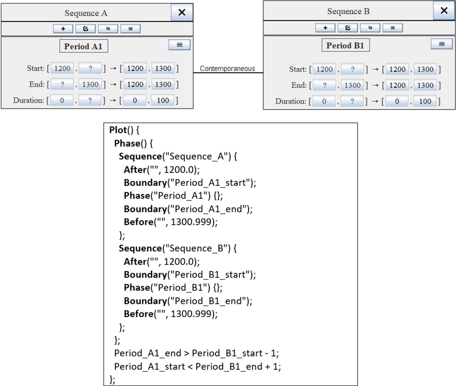
Figure 7 Example of converting a contemporaneity synchronism to OxCal. Radiocarbon dates are omitted for the sake of conciseness. The OxCal constraints corresponding to the ChronoLog synchronism are shown in bold. The +1 and –1 have been added to emulate ChronoLog’s ≥ and ≤ operators using OxCal’s “>” and “<” operators.
Appendix B presents the complete conversion rules from ChronoLog to OxCal.
5. CASE STUDIES
We present three case-studies taken from recent radiocarbon publications. The ChronoLog files of the case-studies are available online on the ChronoLog website at chrono.ulb.be/download/. These case-studies are presented as proofs of concept, to show how use of our method enables users to reach similar results in a straightforward, effortless manner. All the scripts were executed with OxCal version 4.4. The complete OxCal scripts are provided in Appendix C.
5.1. Egyptian 18th Dynasty (Bronk Ramsey et al. Reference Bronk Ramsey, Dee, Rowland, Higham, Harris, Brock, Quiles, Wild, Marcus and Shortland2010; Quiles et al. Reference Quiles, Aubourg, Berthier, Delque-Količ, Pierrat-Bonnefois, Dee, Andreu-Lanoë, Bronk Ramsey and Moreau2013)
Our first example concerns the chronology of the second half of the Egyptian 18th dynasty (Kings Amenhotep II to Horemheb). Several recent studies have reconstructed the ancient Egyptian chronology based on Bayesian radiocarbon models (Bronk Ramsey et al. Reference Bronk Ramsey, Dee, Rowland, Higham, Harris, Brock, Quiles, Wild, Marcus and Shortland2010; Quiles et al. Reference Quiles, Aubourg, Berthier, Delque-Količ, Pierrat-Bonnefois, Dee, Andreu-Lanoë, Bronk Ramsey and Moreau2013; Shortland and Bronk Ramsey Reference Bronk Ramsey and Shortland2013). These models include radiocarbon samples from contexts associated with known kings, as well as Bayesian priors that model the sequence of kings and provide estimates of the durations of their reigns.
We present a simple such model, with data gathered from previous studies (Bronk Ramsey et al. Reference Bronk Ramsey, Dee, Rowland, Higham, Harris, Brock, Quiles, Wild, Marcus and Shortland2010; Quiles et al. Reference Quiles, Aubourg, Berthier, Delque-Količ, Pierrat-Bonnefois, Dee, Andreu-Lanoë, Bronk Ramsey and Moreau2013). Our model features eight kings, five of whom are associated with contemporary radiocarbon samples (the determinations are from Bronk Ramsey et al Reference Bronk Ramsey, Dee, Rowland, Higham, Harris, Brock, Quiles, Wild, Marcus and Shortland2010). All of the kings are given duration ranges, adapted from Quiles et al. Reference Quiles, Aubourg, Berthier, Delque-Količ, Pierrat-Bonnefois, Dee, Andreu-Lanoë, Bronk Ramsey and Moreau2013. In addition, the model features radiocarbon determinations from the tomb of Sennefer (Quiles et al. Reference Quiles, Aubourg, Berthier, Delque-Količ, Pierrat-Bonnefois, Dee, Andreu-Lanoë, Bronk Ramsey and Moreau2013), a tomb dated between the start of Tutankhamen’s reign and the start of Horemheb’s reign. We also add a terminus ante quem (TAQ) of 1200 BCE for the end of the dynasty. This TAQ is very conservative, as it is ca. 100 years after the accepted historical date for the dynasty’s end. Its inclusion in the model is necessary in order to help OxCal start the Monte Carlo Markov Chain (MCMC) algorithm because our model features no radiocarbon determinations for the last two reigns (see Bronk Ramsey Reference Bronk Ramsey2009a: 357–358).
Figure 8 shows the ChronoLog model. The left side displays the sequence of kings, with their duration ranges and the TAQ. The tomb of Sennefer appears on the right side, with two synchronisms that place it between the starts of the reign of Tutankhamun and of Horemheb. The graphical syntax of the ChronoLog model is simple and self-explanatory. Figure 9 presents a sketch of the OxCal script generated by ChronoLog, based on the input bounds (see Appendix C for the full script). The script is fairly classical, with two sequences (kings, Sennefer), and two synchronisms at the bottom. It was generated using a one-year resolution and the “general model” of outlier analysis (see Section 3.1 above), in order to conform to the original publication (Bronk Ramsey et al. Reference Bronk Ramsey, Dee, Rowland, Higham, Harris, Brock, Quiles, Wild, Marcus and Shortland2010). Table 1 presents the results obtained by running the script, compared to those in Bronk Ramsey et al. Reference Bronk Ramsey, Dee, Rowland, Higham, Harris, Brock, Quiles, Wild, Marcus and Shortland2010. Note the close similarity between the two sets of results. The slight variations might stem from the following factors: (1) the latter model was much wider in time, covering the 17th to 21st dynasties, (2) the reign duration constraints are slightly different,Footnote 6 (3) the latter model used a regional offset of 19±5 radiocarbon years (Bronk Ramsey et al. Reference Bronk Ramsey, Dee, Rowland, Higham, Harris, Brock, Quiles, Wild, Marcus and Shortland2010: 1555) absent from our model.

Figure 8 ChronoLog model for the second half of the Egyptian 18th dynasty. All reigns feature a duration estimate adapted from Quiles et al. (Reference Quiles, Aubourg, Berthier, Delque-Količ, Pierrat-Bonnefois, Dee, Andreu-Lanoë, Bronk Ramsey and Moreau2013). The Sennefer tomb is dated to between the start of Tutankhamen and the start of Horemheb. The model includes radiocarbon determinations (from Bronk Ramsey et al. Reference Bronk Ramsey, Dee, Rowland, Higham, Harris, Brock, Quiles, Wild, Marcus and Shortland2010) in all reigns, except Neferneferuaten, Ay and Horemheb. Further radiocarbon determinations are included in the tomb of Sennefer (from Quiles et al. Reference Quiles, Aubourg, Berthier, Delque-Količ, Pierrat-Bonnefois, Dee, Andreu-Lanoë, Bronk Ramsey and Moreau2013). See Appendix C for full details on the model.

Figure 9 Egyptian 18th dynasty: sketch of the OxCal script generated by ChronoLog. The sketch omits radiocarbon determinations and several reigns, for the sake of conciseness (see Appendix C for the full script).
Table 1 Results of the OxCal script generated by ChronoLog, compared to those of Bronk Ramsey et al. (Reference Bronk Ramsey, Dee, Rowland, Higham, Harris, Brock, Quiles, Wild, Marcus and Shortland2010).

This first example was intended to demonstrate the ease of creating a historical sequence (with duration bounds and TPQs/TAQs) and simple synchronization features (tomb of Sennefer) using ChronoLog. Furthermore, the ChronoLog graphical depiction of the model makes it straightforward to read and to modify. Note that the script has been entirely generated by ChronoLog (including the one-year resolution parameter and the outlier analysis code) and can be run by OxCal without further modificationFootnote 7 . Such is also the case for the scripts of the following two case studies.
5.2. Late Helladic to Proto-Geometric Aegean Chronology (Fantalkin et al. Reference Fantalkin, Finkelstein and Piasetzky2015)
We now illustrate the creation of more complex models, that feature archaeological strata contained within cultural phases. Our model is adapted from Fantalkin et al. (Reference Fantalkin, Finkelstein and Piasetzky2015). Their study featured a carbon-based chronology for Aegean cultural phases, from the late Late Helladic IIIB to the Middle Geometric II period, primarily based on Aegean ceramic imports to the Levant. They built a large Bayesian model, featuring 19 archaeological strata contained within 12 cultural phases, as well as termini post and ante quem (Figure 10). For simplicity, we limited the ChronoLog model presented here to the first six cultural phases (LH IIIB to Early Proto-Geometric; see Figure 11).

Figure 10 Bayesian model of Fantalkin et al. (Reference Fantalkin, Finkelstein and Piasetzky2015: 30, their Fig. 2) for Aegean chronology from the late Late Helladic IIIB to the Middle Geometric II.

Figure 11 ChronoLog model for Aegean chronology from the late Late Helladic IIIB to the Early Proto-Geometric (adapted from Fantalkin et al. Reference Fantalkin, Finkelstein and Piasetzky2015). All the synchronisms are of type “A is included in B”.
Fantalkin et al.’s model used nested OxCal phases for modeling inclusion of strata within cultural phases, as is customary in OxCal modeling. However, ChronoLog does not use nesting of phases, but rather inclusion synchronisms (see Figure 17). The generated OxCal script therefore features one (carbon-less) sequence of cultural phases, and several independent sequences for the strata. Inclusion of strata within a cultural phase is represented by the chronological constraints located at the bottom of the script (Figure 12).

Figure 12 Sketch of the OxCal script automatically generated by ChronoLog for the Aegean chronology case-study (see Appendix C for the full script).
Table 2 compares the results of the script with those of the original paper. The two sets of results show good general agreement, but also some discrepancies, which can be explained by the following considerations:
-
1. Our model is smaller than the original one: we truncated the model at the end of Early Proto-Geometric, to ease the presentation.
-
2. Our model uses synchronisms instead of nested phasesFootnote 8 .
-
3. We used a model of sequences that is different from theirs. We use OxCal’s “contiguous model” (Bronk Ramsey Reference Bronk Ramsey2009a: 348–349), which features one boundary between each pair of consecutive phases. Fantalkin et al. rather used the “sequential” model (ibid.), which features two boundaries between consecutive phases, to allow a gap between them. The dates they provide for each transition (Table 2 below) are obtained using the start of the confidence interval of the first boundary, and the end of the confidence interval of the second boundary (Fantalkin et al. Reference Fantalkin, Finkelstein and Piasetzky2015: 35–36).
Table 2 Results of the OxCal script generated by ChronoLog, compared to those of Fantalkin et al. (Reference Fantalkin, Finkelstein and Piasetzky2015: 31, their Table 2).

5.3. Iron I/Iron II Transition in the Southern Levant (Mazar and Bronk Ramsey Reference Mazar and Bronk Ramsey2008)
Our final case-study concerns a radiocarbon model of the Iron I/Iron II transition in the southern Levant (Mazar and Bronk Ramsey Reference Mazar and Bronk Ramsey2008, Model C3). This model uses an Iron I phase, an Iron II phase, and an additional “Late Iron I” phase whose end is synchronized with the end of Iron I (Figure 13). Twenty-two additional phases representing archaeological strata bearing short-lived 14C samples are nested within these three cultural phases. A ChronoLog representation of this model is given in Figure 14. The model uses two ChronoLog sequences: one for Iron I and Iron II, and another one for “Late Iron I.” The end of Iron I and “Late Iron I” are synchronized through a “Simultaneous end” synchronism. Twenty-two additional time-periods (not shown in Figure 14 through lack of space) represent the strata and are connected to the three main time-periods using “inclusion synchronisms,” as in the previous model. A sketch of the OxCal script generated by ChronoLog is given in Figure 15 (see Appendix C for the full script). The script contains the same radiocarbon determinations as in Mazar and Bronk Ramsey’s Model C3, except for two samples (lab nos. HM3 and QS6), which had to be removed in order to reach an agreement index above 60%. The script uses a one-year resolution in order to conform to the original publication. Table 3 compares the results of our script for the Iron I/Iron II transition to those of Mazar and Bronk Ramsey. The results are very close: at 68% we have 949–928 vs. their 948–919, and at 95% we have 958–917 vs. their 963–917. Here, as before, the slight differences can easily be explained by differences in modeling.

Figure 13 Bayesian model for the Iron I/Iron II transition in the southern Levant (Bronk Ramsey Reference Bronk Ramsey2009a: 351, their Figure 7, adapted from Mazar and Bronk Ramsey Reference Mazar and Bronk Ramsey2008, their Figure 2).


Figure 16 Alternative model, imposing the additional constraint: “Late Iron I starts after the start of Iron I”.
Table 3 Results of the OxCal script generated by ChronoLog, compared to those of Mazar and Bronk Ramsey (Reference Mazar and Bronk Ramsey2008: 173, their Figure 1, Model C3).

Finally, we would like to illustrate how easily ChronoLog enables us to enrich a model. For example, we could posit that the “late Iron I” begins after the start of Iron I, which is actually part of the very definition of “late Iron I” but was not represented in the above model. This can be done very easily, by adding one more synchronism between Iron I and “late Iron I,” namely “late Iron I starts after the start of Iron I” (Figure 16). It also shows that ChronoLog permits having more than one synchronism between two given time-periods. This example is given here for illustrative purposes only, as the generated script gave exactly the same result for the Iron I/Iron II transition as the preceding one.
6. CONCLUSION
This paper demonstrated how to generate Bayesian models automatically using ChronoLog, chronological modeling software (Levy et al. Reference Levy, Geeraerts, Pluquet, Piasetzky and Fantalkin2021) freely available online at chrono.ulb.be. ChronoLog enables users with no computer programming skills, or with no knowledge of the OxCal language, to create complex radiocarbon Bayesian models with the help of a user-friendly interface. This approach has the potential to significantly widen the pool of current practitioners of OxCal Bayesian modeling, by making archaeologists less dependent on programmers for building models. For more experienced OxCal users, ChronoLog can represent a significant time saver, allowing them to generate the skeleton of their OxCal scripts automatically, which they can then fine-tune manually. In addition, ChronoLog’s rich library of high-level synchronisms can be particularly useful for helping users build complex Bayesian models. Our three case-studies showed that our approach produces similar results to those obtained with OxCal models written manually. Yet, as often occurs in automatically generated code, the OxCal scripts generated by ChronoLog are sometimes slower than their manual counterparts. This is due to the former scripts using more OxCal boundaries than manual ones. Furthermore, in the case of strata included within cultural periods, our approach based on synchronisms runs slower than OxCal’s classical approach of nested phases (see Section 5.2). Future developments of ChronoLog will focus on optimizing the generated OxCal code to address these shortcomings.
Finally, we intend to add more OxCal functionalities in future versions of ChronoLog, such as non-uniform phases (with features such as Zero_Boundary, Tau_Boundary, and Sigma_Boundary), and more advanced types of outlier analysis than the currently implemented general model (cf. Bronk Ramsey Reference Bronk Ramsey2009b).
ACKNOWLEDGMENTS
The authors would like to thank Prof. Christopher Bronk Ramsey and Mr. Michael Cordonsky for having answered our technical questions about OxCal. They also thank Prof. Gilles Geeraerts for his valuable advice. We also thank two anonymous reviewers and the associate editor for their helpful suggestions. Eythan Levy was supported by the Center for Absorption in Science (Israel Ministry of Absorption), by the Dan David Foundation and by the Rotenstreich Foundation.
Appendix A. Main ChronoLog Synchronisms

Figure 17 The contemporaneity synchronism and special cases thereof. In the images, time flows from above to below.

Figure 18 Additional ChronoLog synchronisms. In the images, time flows from above to below.
Appendix B. Detailed ChronoLog to OxCal Conversion Rules
Table 4 Detailed ChronoLog to OxCal conversion rules (sequences and bounds).

Table 5 Detailed ChronoLog to OxCal conversion rules (synchronisms).

Table 6 Detailed ChronoLog to OxCal conversion rules (radiocarbon dates).

Appendix C. Details of the case studies
Case-study 1: Egyptian 18th Dynasty
Radiocarbon Dates
Table 7 Radiocarbon determinations included in the first case-study (Egyptian 18th dynasty). The radiocarbon determinations for the kings are from Bronk Ramsey et al. Reference Bronk Ramsey, Dee, Rowland, Higham, Harris, Brock, Quiles, Wild, Marcus and Shortland2010 (excluding outlier samples no. 18520, 19550, 19004, 19263, VERA-4686, VERA-4686B, 20482, and 18954). Those of the tomb of Sennefer are from Quiles et al. Reference Quiles, Aubourg, Berthier, Delque-Količ, Pierrat-Bonnefois, Dee, Andreu-Lanoë, Bronk Ramsey and Moreau2013 (“Bouquet 1” only). Dates with an asterisk are combined.


Case-study 2: Late Helladic to Proto-Geometric Aegean Chronology
Radiocarbon Dates
Table 8 Radiocarbon dates for the Aegean chronology from the late Late Helladic IIIB to the Early Proto-Geometric (adapted from Fantalkin et al. Reference Fantalkin, Finkelstein and Piasetzky2015: 28, their Table 1). Dates with an asterisk are combined.


Case-study 3: Iron I/Iron II Transition in the Southern Levant
Radiocarbon Dates
Table 9 Radiocarbon dates for the Iron I/II transition in the southern levant (adapted from Mazar and Bronk Ramsey Reference Mazar and Bronk Ramsey2008, model C3, excluding additional samples HM3 and QS6). In cases of discrepancies (samples MG5, MG9, Y1, Y3, GrN-26121, GrN-18825) between Mazar and Bronk Ramsey’s OxCal script (p. A23) and their table (Table 2, p. 164), we have followed the script. Regarding the Tel Miqne samples (originating in Stratum V but initially reported as coming from Stratum IV), see Mazar and Bronk Ramsey Reference Mazar and Bronk Ramsey2008, note 3. Dates with an asterisk are combined.


 Open access