


INTRODUCTION
During the last ice age, large volumes of water were stored in the continental ice caps. As a consequence, sea levels were roughly 100 m lower than today. At that time, the southern North Sea was a diverse landscape inhabited by a rich fauna. It was in fact part of the Mammoth Steppe (Mol et al. Reference Mol, Post, Reumer, van der Plicht, de Vos, van Geel, van Reenen, Pals and Glimmerveen2006a, Reference Mol, de Vos, Bakker, van Geel, Glimmerveen, van der Plicht and Post2008, Reference Mol and Post2010a; Lister and Bahn Reference Lister and Bahn2007; Kuitems Reference Kuitems2020), and the area is considered a unique and rich heritage site that was inhabited by humans, in particular during the Mesolithic (Peeters Reference Peeters, Benjamin, Bonsall, Pickard and Fischer2011; Roebroeks Reference Roebroeks2014; Meiklejohn et al. Reference Meiklejohn, Niekus and van der Plicht2015; van der Plicht et al. Reference van der Plicht, Amkreutz, Niekus, Peeters and Smit2016). Recent investigations have increased our insights into geographical aspects of this now submerged landscape (Gaffney et al. Reference Gaffney, Thomsen and Fitch2007; Sturt et al. Reference Sturt, Garrow and Bradley2013; Cohen et al. Reference Cohen, Gibbard and Weerts2014; van Heteren et al. Reference van Heteren, Meekes, Bakker, Gaffney, Fitch, Gearey and Paap2014). Nevertheless, still a lot of unanswered questions exist about the animals and people who occupied the area despite the large quantities of fossil bones and occasional artifacts extracted from the seabed (Glimmerveen et al. Reference Glimmerveen, Mol and van der Plicht2006; Mol et al. Reference Mol, de Vos, Bakker, van Geel, Glimmerveen, van der Plicht and Post2008, Reference Mol and Post2010a).
The main reason is that most of the finds derive from unknown stratigraphical, geographical, and archaeological contexts (Peeters Reference Peeters, Benjamin, Bonsall, Pickard and Fischer2011). As a result of natural erosion and sedimentation, finds are not in situ. In addition, the vast majority of finds has been brought up in fishing nets or came ashore in sand dredged from the seabed for the purpose of coastal reinforcement and land reclamation. An example of the latter is the Zandmotor (sandmotor) located on the coast near Den Haag (The Hague). But also several zones in the southern North Sea, for instance the Brown Bank and Eurogeul, are known as palaeontological and/or archaeological “hot spots” which have been subject to targeted “fishing” expeditions. A rare location where research of in situ contexts has been conducted is Rotterdam-Maasvlakte in the Netherlands (Moree and Sier Reference Moree and Sier2015). Figure 1 shows a map of the North Sea with relevant locations.

Figure 1 Map of the North Sea showing the most relevant find locations of fossil bones: M: Maasvlakte, Z: Zandmotor, B: Belgium, D: Germany, DK: Denmark, F: France, N: Norway, NL: Netherlands, UK: United Kingdom, A: Amsterdam, L: London, R: Rotterdam.
A major aspect concerns the establishment of the age of the fossil finds. Over the last decades, many samples have been submitted for 14C dating, which has resulted in an important and unique series of dates. For 14C dating, also the stable isotope 13C is measured for fractionation correction; analysis of the stable isotope 15N of the dated bone collagen was introduced later, in the 1990s. Both stable isotopes are proxies used for reconstruction of, and for information on (palaeo)climatological and environmental change (e.g., Fry Reference Fry2008). A good example concerns the Mesolithic hunter-gatherers of Doggerland. Analysis of the 13C and 15N isotope contents of their bones indicates that their major food resource was freshwater fish (van der Plicht et al. Reference van der Plicht, Amkreutz, Niekus, Peeters and Smit2016).
This contribution presents an overview of fossil bones analyzed for their natural isotopes. It comprises more than 200 animal bone dates. It provides a catalog of samples measured over the last decades, with 14C dates measured both conventionally and by AMS, most of them also providing the stable isotopes 13C and 15N. The majority of the measurements were done in Groningen. For the purpose of completeness these were supplemented by available data from other laboratories. The isotopic data provide a major contribution towards an integrated understanding of the North Sea in the past. Detailed palaeontological, archaeological, and geophysical interpretations of the North Sea finds can be found in the extensive literature.
METHODS
Techniques and Conventions
For isotope analysis, the collagen fraction of the bone is isolated. This is done generally by following an improved version of the method originally developed by Longin (Reference Longin1971). In brief, the sample is first entirely released from bioapatite and contaminants such as humic acids. Subsequent heating at 90°C causes gelatinization of the collagen (Mook and Streurman Reference Mook and Streurman1983; Mook and van de Plassche Reference Mook, van de Plassche and van de Plassche1986). For a complete description of sample pretreatment aspects we refer to Dee et al. (Reference Dee, Palstra, Aerts-Bijma, Bleeker, de Bruijn, Ghebru, Jansen, Kuitems, Paul, Richie, Spriensma, Scifo, van Zonneveld, Verstappen-Dumoulin, Wietzes-Land and Meijer2020).
The list of data comprises measurements performed over decades at 3 separate laboratories: conventional (until 2011, Groningen code GrN) and AMS (by 2 machines: Tandetron 1994–2017, code GrA and Micadas, since 2017, code GrM). Large samples have been measured by radiometry. The collagen is combusted to produce CO2; the 14C activity is measured using proportional counters. The δ13C ratio is measured by mass spectrometry (IRMS). For more technical details of the conventional method we refer to Mook and Streurman (Reference Mook and Streurman1983) and Cook and van der Plicht (Reference Cook and van der Plicht2013).
Small samples (and large ones since 2011) are measured by AMS. The first AMS was a 2.5MV Tandetron (van der Plicht et al. Reference van der Plicht, Wijma, Aerts, Pertuisot and Meijer2000). The present AMS is a Micadas system (Synal et al. Reference Synal, Stocker and Suter2007). Both employed a combination of Elemental Analyser/Mass Spectrometer (EA-IRMS). The EA combusts the collagen into CO2 which is subsequently reduced into graphite (Aerts et al. Reference Aerts-Bijma, van der Plicht and Meijer2001). The graphite is pressed into targets, mounted in a sample wheel before it is loaded into the ion source of the machine. The IRMS measures the stable isotope ratios δ13C and δ15N.
Stable isotope concentrations are measured by mass spectrometry, based on molecular gases. The stable Carbon isotope (13C) content of the sample is measured in CO2 by IRMS (isotope ratio mass spectrometry) upon combustion of the pre-treated 14C sample material (such as collagen, prepared from fossil bone). Thus, the same CO2 is used for both isotope measurements, 13C and 14C dating—either by AMS or by the conventional method. For the nitrogen isotope 15N, also IRMS is used. In this case, N2 gas prepared from the same collagen sample is used.
The stable isotopic content of the samples is expressed in delta (δ) values, which are defined as the deviation (expressed in per mil) of the rare to abundant isotope ratio from that of a reference material where δ = [(aR/bR) sample /(aR/bR) reference –1]; aR is the rare-, and bR the abundant isotope ratio. For carbon, the reference material is belemnite carbonate (V-PDB); for nitrogen, the reference is ambient air (Mook Reference Mook2006). The analytical error is 0.1‰ and 0.2‰ for δ13C and δ15N, respectively. The 14C dates are reported in BP by convention (Mook and van der Plicht Reference Mook and van der Plicht1999), using the oxalic standard and Libby halflife and including normalization for fractionation. The 14C dates are calibrated using IntCal20 (Reimer et al. Reference Reimer, Austin, Bard, Bayliss, Blackwell, Ramsey, Butzin, Cheng, Edwards, Friedrich, Grootes, Guilderson, Hajdas, Heaton, Hogg, Hughen, Kromer, Manning, Muscheler, Palmer, Pearson, van der Plicht, Reimer, Richards, Scott, Southon, Turney, Wacker, Adolphi, Büntgen, Capano, Fahrni, Fogtmann-Schulz, Friedrich, Köhler, Kudsk, Miyake, Olsen, Reinig, Sakamoto, Sookdeo and Talamo2020) and OxCal software (Bronk Ramsey Reference Bronk Ramsey2009). Calibrated dates are reported in calBP, i.e., calendar age relative to 1950 AD.
Bone Quality Aspects
Bone collagen is sensitive to degradation. The most common indicators for collagen integrity are the carbon and nitrogen extraction yields of the collagen, denoted as %C and %N, respectively. These numbers are provided by the mass spectrometer. Also, the atomic C/N ratio, C/N = (%C/%N) × (14/12) is a widely accepted quality parameter. Based on comparison with the chemical composition of collagen extracted from fresh bone using the same purification treatment, the carbon content of genuine collagen should be around 30-40 % and its nitrogen content around 11–16% for reliable results (van Klinken Reference van Klinken1999). The C/N ratio for well-preserved bone collagen is 2.9–3.6 (DeNiro Reference DeNiro1985; Ambrose Reference Ambrose1991). The weight proportion of the extracted collagen in relation to the initial sample weight (% yield) is preferably minimally 0.5 (van Klinken Reference van Klinken1999). For fresh bone, this number is about 20%.
In terms of contamination, one can calculate how much contamination is needed to explain aberrant dates. It obviously depends on the age of the contaminant, which theoretically can be any age between modern and fossil. Let us assume here modern contamination, then a contamination of 1% modern Carbon a sample of 50,000 BP will be measured as 35,000 BP. More examples can be found in Mook and Streurman (Reference Mook and Streurman1983) and Mook and van de Plassche (Reference Mook, van de Plassche and van de Plassche1986), both written for the conventional dating method, using large samples. For our example, 1% foreign Carbon for a 1-gram sample is 10 mg, which is relatively much. The same calculations apply to AMS but the samples are much smaller. Here, a contamination of 1% foreign Carbon for a 1 mg sample is only 10 μg; therefore, AMS is much more sensitive for contamination (Lanting and van der Plicht Reference Lanting and van der Plicht1994).
In natural circumstances, contamination can be caused by processes such as degradation which can enable invasion of carbon containing matter from the environment (Mook and Streurman Reference Mook and Streurman1983). This is particularly true for Pleistocene samples. We do not have an example where this is clearly shown, because of the lack of context for the North Sea samples. The key for successful dating is quality control, in particular the Carbon content of the collagen (Mook and Streurman Reference Mook and Streurman1983; Olsson Reference Olsson2009), later supplemented by the Nitrogen content. Also, the δ13C and δ15N values must be in certain ranges (van Strijdonck et al. Reference van Strijdonck, Nelson, Combré, Bronk Ramsey, Scott, van der Plicht and Hedges1999). For example, a δ13C value of say –25‰ for bone can be suspect, in particular when the C content is low; contamination with material having low δ13C values, like soil components, is then not unlikely. When the conservation circumstances are excellent, like in the permafrost, the collagen is usually perfect for dating, allowing dating to very old ages (slightly over 50,000 BP). An example is the Arilakh mammoth (Mol et al. Reference Mol, Tikhonov, van der Plicht, Kahlke, DeBruyne, van Geel, Pals, de Marliave and Reumer2006b). Together with discussions concerning which samples should be used as blank (background) for the 14C method, made us argue to set the upper limit for bone dating at 45,000 BP. For details see van der Plicht and Palstra (Reference van der Plicht and Palstra2016).
RESULTS
The vast majority of data is in this overview is obtained by the Groningen laboratory. Limited data for the North Sea are available from other laboratories, which are included here to provide a date list for the North Sea which is as complete as possible. The laboratories can be recognized by internationally assigned laboratory codes as follows:
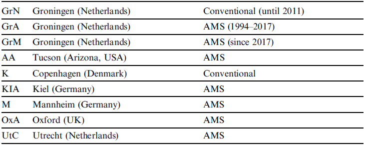
Some codes/laboratories are no longer in use or active today: GrN, GrA, K, and UtC (see the list of lab codes at www.radiocarbon.org).
The main result of 14C measurement is, of course, the dating itself: a direct measurement of the age of the sample, which is otherwise difficult or impossible to establish. This is especially true for the North Sea finds because there is in general a lack of context like stratigraphy and/or associations. The results are shown in Tables 1 and 2 (see Appendix). They show the results for animal bones, sorted to 14C age. Table 1 shows the animal bone results for ages older than the Holocene era; Table 2 for the Holocene era.
Laboratory code, locality, 14C age and its uncertainty, species and skeletal element are shown, as well as the C and N contents and stable isotope ratios δ13C and δ15N of the collagen, when available. Some dates close to the dating limit are reported with asymmetric uncertainties, shown as σ(–) and σ(+). The 14C dates are calibrated using the IntCal20 curve (Reimer et al. Reference Reimer, Austin, Bard, Bayliss, Blackwell, Ramsey, Butzin, Cheng, Edwards, Friedrich, Grootes, Guilderson, Hajdas, Heaton, Hogg, Hughen, Kromer, Manning, Muscheler, Palmer, Pearson, van der Plicht, Reimer, Richards, Scott, Southon, Turney, Wacker, Adolphi, Büntgen, Capano, Fahrni, Fogtmann-Schulz, Friedrich, Köhler, Kudsk, Miyake, Olsen, Reinig, Sakamoto, Sookdeo and Talamo2020) and are given as the 95% confidence range in calBP. The numbers are rounded to significant values.
The tables also include a parameter “quality” which we have defined as follows. Accepted dates are indicated by “a”. They all meet the established quality aspects concerning C and N. The label “1” means that not all criteria are known. For example, for samples measured by other laboratories in we only have the 14C dates and not the other data. Mostly, the δ13C values are not published or otherwise available. The label “2” means that not all criteria are strictly met, but the outcomes are reasonable. For example, a C/N ratio of 2.8 is strictly taken not acceptable. But one has to take into account that the C% and N% measurements from which the C/N ratio is calculated are not very precise. In practice, there is no good reason for rejection. The label “3” means that only the C isotopes are measured (14C and 13C). This is related to the historical developments of the radiocarbon method. During the early decades of the method, the N isotopes of collagen has not been measured. This applies to almost all conventional dates and the early AMS dates. The measurement of N isotopes gradually became standard since the 1990s. The measurements that are “crossed out” are shown for completeness but rejected because of unacceptable sample quality. In all cases, we have used 0.5% collagen yield of the raw bone material as acceptance threshold.
In Figure 2 we show an overview of all dated bones, sorted taxonomically. A grand total of 144 Pleistocene and 71 Holocene accepted faunal dates (including duplicates) is represented. Figure 2 also includes human bone data from the North Sea; these are not further discussed here (see van der Plicht et al. Reference van der Plicht, Amkreutz, Niekus, Peeters and Smit2016). In Figure 2, the 14C ages (BP) are given instead of calibrated dates (calBP) to avoid reservoir effect ambiguities and still existing uncertainties in the oldest part of the calibration curve. The marine species are subject to a reservoir effect. This also applies to the giant auk. For the Holocene North Sea, for the reservoir effect a general number of 400 years can be taken. For the Pleistocene this number can vary significantly, depending on time and location. For a detailed discussion see Heaton et al. (Reference Heaton, Köhler, Butzin, Bard, Reimer, Austin, Bronk Ramsey, Grootes, Hughen, Kromer, Reimer, Adkins, Burke, Cook, Olsen and Skinner2020) and references therein. For non-marine aquatic species (in terms of diet), an unknown reservoir effect applies. This is the case for the otter. Also, humans with a significant subsistence of freshwater/marine fish have an unknown reservoir effect.
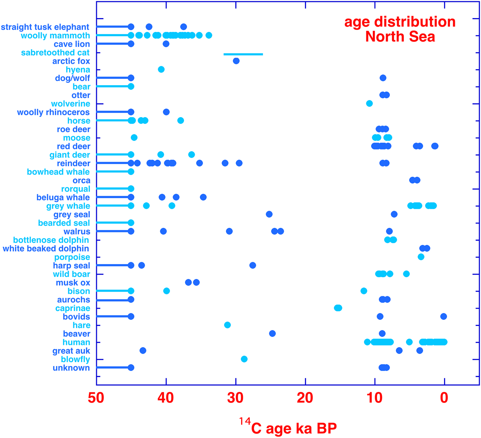
Figure 2 Age distribution of all dated bones from the North Sea, organised by species or taxonomical family. The horizontal lines at the left side of the figure correspond to ages larger than 45,000 BP. Dates reported as finite and older than 45,000 BP are truncated at 45,000 BP.
DISCUSSION: RADIOCARBON DATES OF THE FAUNA
Some General Observations for the 14C Dates
The data (Tables 1–2 and Figure 2) show that the majority (about 2/3) of the fossils date to the Pleistocene. These are all faunal samples and include true 14C dates and ages which are infinite on the 14C time scale. A second group (about 1/3) represent the Holocene. These concern both human and animal fossil bones, including artifacts made of bone. It appears that the LGM (Last Glacial Maximum) period around 20,000 BP seems to be more less devoid of fossils. For the Holocene there are also human fossil bones; there is a group dating to the Mesolithic, and a (larger) group which is (sub)recent. For these data we refer to van der Plicht et al. (Reference van der Plicht, Amkreutz, Niekus, Peeters and Smit2016). After the Mesolithic the region became uninhabitable due to the sea level rise. Concerning the Glacial record, we note here a particular important example GrA-58271, a Late Glacial parietal bone which dates 11,050 ± 50 BP and is described in detail by Amkreutz et al. (Reference Amkreutz, Verpoorte, Waters-Rist, Niekus, van Heekeren, van der Merwe, van der Plicht, Glimmerveen, Stapert and Johansen2018). There is one Neandertal skull find known from the North Sea (Hublin et al. Reference Hublin, Weston and Gunz2009). Unfortunately, as this sample did not contain collagen, it could not be dated. All other human bones assessed as possibly Neandertal based on their patina were dated as Mesolithic.
Terrestrial animals dated thus far are straight tusked elephant, woolly mammoth, cave lion, saber-toothed cat, arctic fox, hyena, dog/wolf, bear, otter, wolverine, woolly rhinoceros, horse, roe deer, moose, red deer, giant deer, reindeer, wild boar, musk ox, bison, aurochs, caprinae, other bovids, hare, and beaver. Marine animals are bowhead whale, orca, common rorqual, beluga whale, grey whale, grey seal, bearded seal, walrus, bottlenose dolphin, white beaked dolphin, porpoise, and harp seal. The dataset contains one bird species (great auk).
It is of interest here to note that Late Pleistocene and Early Holocene mammals from two different sites in the Netherlands show many similarities. The faunal composition of the dredged site De Groote Wielen (near Den Bosch) and the Eurogully (North Sea) is almost identical. The 14C dates show that the mammoth fauna are more or less of the same age. The results from De Groote Wielen, in particular for woolly mammoth (Mammuthus primigenius) and woolly rhinoceros (Coelodonta antiquitatis) can be found in Mol et al. (Reference Mol, Verhagen and van der Plicht2010b).
However, aspects such as taphonomic processes, choices for sediment used for sand suppletion projects, mesh size of fishing nets, detection of finds by (often amateur) collectors, and the glamour of specific finds dramatically determine the type of North Sea finds that are finally submitted for radiocarbon dating. Hence, the composition of the current dataset is biased, which affects the representation of species and periods. For instance, small, fragile fish and bird bones are just sporadically submitted for radiocarbon dating. First of all, classical, precise excavation and sieving methods cannot be applied within the North Sea area, limiting the recovery of smaller sized finds. Moreover, often the collagen of such remains does not preserve well enough for dating purposes.
Samples of cervids are represented in relatively high numbers in the radiocarbon dataset. Many of these are modified antlers. But also artifacts made of cervid bones and skeletal elements of bovids and horses have been submitted for age determination. A prime example is a decorated, Late-Glacial bovid metatarsus which dated 11,560 ± 50 BP (GrA-28364) see Amkreutz et al. (Reference Amkreutz, Verpoorte, Waters-Rist, Niekus, van Heekeren, van der Merwe, van der Plicht, Glimmerveen, Stapert and Johansen2018).
Many finds come from a limited number of regions from the North Sea area, specifically locations that are frequently exploited by fishermen and that are suitable for sand extraction purposes. Indeed, more than a third of the samples come from the important fishing areas Eurogully and the Brown Bank (see Figure 1). Also, a large part comes from the Dutch province Zuid-Holland, where many large sand suppletion projects took place in recent years, in particular Maasvlakte and Zandmotor (Figure 1).
Although this dataset reflects a biased composition of dwellers of the North Sea area in the past, it gives insight in aspects such as species present in different periods and chemical conservation of fossil remains, helps to solve geological puzzles of the North Sea bottom, and reveals some spectacular discoveries.
Context of the Material
A difficult issue has always been the context of the finds from the North Sea. Only recently, a detailed stratigraphic framework has been made for the Eurogeul region (Hijma et al. Reference Hijma, Cohen, Roebroeks, Westerhoff and Busschers2012) and for a small region offshore of the Maasvlakte area (Busschers et al. Reference Busschers, Westerhof and van Heteren2013). The defined lithostratigraphic units show signs of repeated, severe reworking during various fluviatile and/or marine depositional phases. Therefore, is likely that none of the North Sea assemblages, including the dated samples discussed in this paper, are pristine and free from mixing.
The geological framework presented by Hijma et al. (Reference Hijma, Cohen, Roebroeks, Westerhoff and Busschers2012), even implies that all Late Pleistocene terrestrial mammals dating older than around 30,000 years must have been redeposited from their original location. However, overall, the skeletal remains from the North Sea are well preserved with just few signs of weathering and little or no rounding (Kuitems et al. Reference Kuitems, De Loecker, van Kolfschoten, Borst, van Doesburg, van der Es, Opdebeeck, Otte, Reumer, van Tongeren, Weerts and Wesselingh2013a). Such taphonomic characteristics indicate that the skeletal material did not lie on the surface for long, nor was it transported over large distances. Therefore, many finds may derive from eroded, large lumps of such reworked sediments (Kuitems et al. Reference Kuitems, van Kolfschoten, De Loecker and Busschers2013b).
Besides the depositional history of the material, the way the fossils have been retrieved hampers assigning palaeontological and archaeological finds to a precise stratigraphic unit. That is, most fossils of large mammals are collected during fishing expeditions (Mol et al. Reference Mol, de Vos, Bakker, van Geel, Glimmerveen, van der Plicht and Post2008; Mol and Post Reference Mol and Post2010a). The rough location of the ship was reported along with many of the samples that were found in fishing nets. But, even the most detailed data available on location and depth of the nets are far from precise enough to link a find to a specific stratigraphical layer (Kuitems et al. Reference Kuitems, van Kolfschoten, De Loecker and Busschers2013b). However, combining the radiocarbon dates, ship’s coordinates, geological information and knowledge of ecological preferences and restrictions of species, a number of finds can be assigned to a specific lithological unit. Below, selected results of the isotope date list for the North Sea fossil bones are discussed and highlighted in more detail.
Unique Samples
Unique finds are first finds of certain species of the Mammoth steppe in the North Sea. Among these is a first find of a hare (Lepus Sp.) from the bottom of the North Sea, found at the Zandmotor. It is a mandible, 14C dated to 31,140 (–190, +200) BP (GrA-54021). For more details we refer to Mol and van der Plicht (Reference Mol and van der Plicht2012a). This result represents a first such old date for this species for the North Sea.
Also finds of bones from an otter (Lutra lutra) yield the first dates for this species from the North Sea. They were recovered from the sand suppletion area for the Maasvlakte (Mol and van der Plicht Reference Mol and van der Plicht2012b). Two specimens date to the Early Holocene: 8825 ± 45 BP (GrA-52432) and 8300 ± 40 BP (GrA-52433). This result provides a clear answer to the question whether these animals date to the mammoth fauna or not.
Another first age-establishment for a species in this particular area concerns an arctic fox (Alopex) from the Zandmotor, in the suppleted sand originating from the Eurogully (Langeveld et al. Reference Langeveld, Mol and van der Plicht2018). It is dated to 29,900 (–490, +550) BP (GrA-69520). We note that an even younger arctic fox is known from De Groote Wielen near ’s-Hertogenbosch in the southern Netherlands, about 90 km inland. The 14C date is 21,890 ± 100 BP (GrA-35484; Verhagen and Mol Reference Verhagen and Mol2009).
A series of 11 fossil bones from the giant auk (Pinguinus impennis) from the North Sea region was submitted for 14C dating (Langeveld Reference Langeveld2015). Unfortunately, only three samples appeared datable; the collagen yield of the others was too low. The collagen of the three analysed samples was of good quality (see C and N parameters, Table 1 and 2). Two samples from the Zandmotor dated Holocene, the youngest 3505±45 BP (GrA-65546). One bone dated Pleistocene: 43,290 (–380, +400) BP (GrA-64453). The latter was found on the beach of Hoek van Holland. The stable isotope (δ13C and δ15N) results of the three auk samples indicate a pure marine diet, as expected. That means that the dates need to be corrected for the reservoir effect. For the Holocene the correction is 400 years. Thus, the youngest sample is 3105 14C years old, which calibrates into 1425–1300 BC.
A unique find of importance is a fossil bone (mandible with teeth) of a sabertoothed cat (Homotherium) from the Brown Bank. A series of six samples was dated by AMS in Utrecht, resulting in a final date of ca. 28,000 BP (Reumer et al. Reference Reumer, Rook, van der Borg, Post, Mol and de Vos2003). These six dates range between 26,700 and 31,300 BP, with uncertainties ranging between 220 and 400 BP. A few samples of mandible and tooth were dated with varying results in δ13C and 14C age. Hence, the six dates cover a significant range, which is indicated in Figure 2 as a horizontal bar because it concerns here only one specimen. However, no further quality parameters of the collagen are available.
Relevant Dates for Non-Bone Samples
There are a few samples with a North Sea context that were radiocarbon dated which are not bone or another skeletal part, but are relevant: wood artifacts, fly pupae, coprolites, and plant remains. Here we discuss only finds which are faunal related.
Fly pupae (Protophormia terraenovae) were found in a skull from a woolly mammoth dredged from the Eurogully. They were dated by 14C to 28,740 (–180, +190) BP (GrA-50454; Table 1) (van der Plicht et al. Reference van der Plicht, Post and Mol2012). Like many other 14C dates, this is younger than stratigraphic inferences for the Eurogully (Hijma et al. Reference Hijma, Cohen, Roebroeks, Westerhoff and Busschers2012). The importance of this fly pupae date that it is not obtained from fossil bone. Pleistocene bone collagen is often a subject of deliberations in terms of degradation and/or contamination (e.g., van der Plicht and Palstra Reference van der Plicht and Palstra2016). There is no reason at all to “suspect” the fly pupae date in this respect. We note that there is one other fly pupae date known from “de Groote Wielen” near Den Bosch, the Netherlands, that was found in association with Late Pleistocene mammal bone. The date is 26,660 ± 150 BP (GrA-35816) (Verhagen and Mol Reference Verhagen and Mol2009). This date shows the same general timerange as that of the Eurogully.
A few coprolites of Hyena (Crocuta crocuta) are found, and dating has been attempted. However, because of the nature of the sample material this appeared problematic. One coprolite (found on the Brown Bank) contained a small bone and a small piece of wood. The latter dates to 18,310 ± 150 BP (GrA-59740). The bone appeared not datable. A coprolite found on the Maasvlakte (in sand originating from the Eurogully) was dated as “organic matter,” yielding a 14C age of 35,050 (–240, +250) BP (GrA-56323). The C content was low (4.9%), the δ13C value –16.43‰.
A recent find is a molar from a giant deer (Megaloceros giganteus). It was found in sandy deposits of the North Sea, about 10 km west of the present coastline. Unfortunately, the collagen preservation of the molar appeared very poor. This sample is not included in the datatable and figures. However, plant remains were preserved in the deep folds of the molar. This shows that the animal foraged in a steppe environment, eating Artemisia. For details we refer to van Geel et al. (Reference van Geel, Sevink, Mol, Langeveld, van der Ham, van der Kraan, van der Plicht, Haile, Rey-Iglesia and Lorenzen2018). The plant remains are 14C dated to 38,750 (–290, +300) BP (GrA-68256), corresponding to Greenland Interstadial 11.
Anomalous 14C Dates
A striking example is a worked reindeer bone with cut marks displaying a human face. Archaeologically this is potentially a sensational sample, believed to date to the Mesolithic. But it dated to 1310 ± 60 BP (GrA-20291). Technically, this was a problematic sample because the bone had been treated with preservatives, and the material was very delicate. It was established by radiocarbon that the artifact was not as old as was hoped; it is not related to ancient people living in what is today the North Sea area. A duplicate dating yields essentially the same date (GrA-22093, 1370 ± 40 BP). This pair of 14C dates was the reason to change the determination from reindeer to red deer. Assuming the contamination was removed adequately, of course. The preservative applied is known as Stelfon, which is of fossil origin (i.e., does not contain 14C). So, in contrast to most collagen-containing contaminants, if any contamination was left on the material after pretreatment it measures older than its actual age, its true age being even more recent.
Another anomalous date concerns a “goat-like animal” (Caprinae) from the Brown Bank, which could not be further identified. It dates to the Late Glacial: 15,190 ± 60 BP (GrA-38211) which is impossible, or at least not very likely based on present palaeontological understanding. The sample was dated again, even in threefold, all with the same result (Table 1). There is no reason to doubt the dating; there are no signs of contamination, and the sample quality parameters are good. In theory the species identification could be problematic but that is not known. This sample is a mystery which still remains to be resolved.
Issues Near the 14C Limit
Many of the (Late) Pleistocene fossils belonged to typical so-called mammoth steppe fauna. Moreover, a large number of Pleistocene fossils are from marine mammals. The set of 14C dates for large marine mammals have raised questions, which still need to be resolved. That is, many whales date between 35,000 and 45,000 BP and walruses between 25,000 and 30,000 BP. However, following Hijma et al. (Reference Hijma, Cohen, Roebroeks, Westerhoff and Busschers2012), the marine fauna should be about 60–85,000 years old. Therefore, these 14C dates have been criticized (Rijsdijk et al. Reference Rijsdijk, Kroon, Meijer, Passchier, van Dijk, Bunnik and Janse2013). Could contamination possibly cause anomalously young dates such that fossils of say 80,000 years old date 40,000 in the laboratory? This question has been raised earlier for the Homotherium (dating around 28,000 BP) and Elephas antiquus (37,440 ± 310 BP, GrA-25815). These samples should perhaps be redated for confirmation, applying compound specific dating (Devièse et al. Reference Devièse, Comeskey, McCullagh, Bronk Ramsey and Higham2018).
The above was a motivation to study in depth some technical issues concerning 14C dating of Pleistocene (i.e., “old”) samples. This concerns laboratory intercomparisons, backgrounds, contamination and pretreatment. A series of mammoth bones from the North Sea has been investigated for this purpose. This “test series” resulted in valid dates which are shown in Tables 3 and 4 and concerns GrA-56655, 56656, 55658, 56660, 56661, 56662, 56664, 56674, 56675, and 56676. Incidentally, of our test series GrA-56660 (a mammoth humerus from the Eurogully) showed bite marks of Hyena. Hence, the 14C date provides a date for this species, i.e., Crocuta crocuta spelaea, as well.
Radiocarbon laboratories regularly organize an exchange of samples varying in age and material to compare dating protocols (Scott et al. Reference Scott, Cook and Naysmith2010). The latest intercomparison program is known as SIRI (Sixth International Radiocarbon Intercomparison; see www.radiocarbon.org). The sample dated as GrA-56658 is already in use for the purpose and is now known as sample B for SIRI. Other bones from the North Sea bones were also shipped to the Glasgow laboratory (the coordinating laboratory for 14C intercomparisons) for possible future use.
Some samples are just lightly touched by glue, which is supposedly efficiently removed, in particular with an extra chemical cleaning called “Soxhlet” (Bruhn et al. Reference Bruhn, Duhr, Grootes, Mintrop and Nadeau2001). Such contamination was applied to a series of samples from Great Yarmouth (6 miles east off the coast): GrA-39962, 39964, 39965, 39966, and 39121. Indeed, the resulting collagen parameters are well in their acceptable ranges, and the dates appear reasonable. For more details concerning the Soxhlet procedures applied in Groningen we refer to Dee et al. (Reference Dee, Palstra, Aerts-Bijma, Bleeker, de Bruijn, Ghebru, Jansen, Kuitems, Paul, Richie, Spriensma, Scifo, van Zonneveld, Verstappen-Dumoulin, Wietzes-Land and Meijer2020).
Apart from the official intercomparison program which includes samples of all ages and materials, Pleistocene bones are often dated by more than one laboratory to compare protocols. This is particularly done for samples which are unique. Examples can be found in the literature (Semal et al. Reference Semal, Rougier, Crevecoeur, Jungels, Flas, Hauzeur, Maureille, Germonpre, Bocherens, Pirson, Cammaert, de Clerck, Hambucken, Higham, Toussaint and van der Plicht2009; Crevecoeur et al. Reference Crevecoeur, Bayle, Rougier, Maureille, Higham, van der Plicht, De Clerck and Semal2010; Maroto et al. Reference Maroto, Vaquero, Arrizabalaga, Baena, Baquedano, Jorda, Julia, Montes, van der Plicht, Rasines and Wood2012; Fiedel et al. Reference Fiedel, Southon, Taylor, Kuzmin, Street, Higham, van der Plicht, Nadeau and Nalawade-Chavan2013; Huels et al. Reference Huels, van der Plicht, Brock, Matzerath and Chivall2017; Kuzmin et al. Reference Kuzmin, Fiedel, Street, Reimer, Boudin, van der Plicht, Panov and Hodgins2018). Of particular interest here is the so-called ultrafiltration method (Bronk Ramsey et al. Reference Bronk Ramsey, Higham, Bowles and Hedges2004) which was introduced to further purify (i.e., remove remaining contaminants) from bones treated by the classic Longin (Reference Longin1971) method. However, the effectiveness of ultrafiltration is not without controversy (Huels et al. Reference Huels, Grootes and Nadeau2009; Fülöp et al. Reference Fülöp, Heinze, John and Rethemeyer2013; Minani et al. Reference Minami, Yamazaki, Omori and Nakamura2013).
The laboratory intercomparisons show that for good quality bone, no additional treatments are necessary (van der Plicht and Palstra Reference van der Plicht and Palstra2016). Furthermore, we mention here a relatively new development: compound specific dating. Separated amino acids from collagen, in particular hydroxiproline (known as HYP) are the most reliable datable fraction of (partially) degraded bone (Devièse et al. Reference Devièse, Comeskey, McCullagh, Bronk Ramsey and Higham2018).
Another important methodological aspect is the dating limit of the 14C method, and reporting dates close to that limit. The measurement errors become asymmetric, leading to the so-called 2-sigma criterion: when the measured activity becomes smaller than 2 times its measurement error, the age is given as this limit (Olsson Reference Olsson1989; van der Plicht and Hogg Reference van der Plicht and Hogg2006). As stated above, a proper background determination is essential as well. In any case, dates like KIA-25281 reported as a finite number 54,010 (–2630, +3940) BP (see Table 1) we consider not realistic.
DISCUSSION: STABLE ISOTOPES OF THE FAUNAL BONES
Along with radiocarbon, stable carbon and often nitrogen isotopes have been measured for many of the organic remains. The stable isotope (13C, 15N) signal of fossil animal bones is a powerful tool for investigating ancient environments, ecosystems, and the reconstruction of the diet and ecological preferences of species (e.g., Drucker et al. Reference Drucker, Hobson, Ouellet and Courtois2010). For animals and humans, the isotopic values of fossil distinguish herbivores, omnivores, carnivores, C3 and C4 plant consumers, and terrestrial and aquatic diets—to mention the main categories. Such analyses are based on the principle that the organic tissues of an organism (bone collagen and teeth) reflect the composition of the food and water the organism ingested during its life (Kohn Reference Kohn1999; Fry Reference Fry2008). Well known is the large distinction in δ13C values between C3 and C4 plants, which utilize a different photosynthesis process. These values are reflected in the tissues of consumers (e.g., Vogel and van der Merwe Reference Vogel and van der Merwe1977; Fry Reference Fry2008).
Distinctive δ15N values are observed between trophic levels. The isotopic enrichment of the δ15N value is larger than that of δ13C, about 3–5‰ for each trophic level shift (Bocherens and Drucker Reference Bocherens and Drucker2003; Hedges and Reynard Reference Hedges and Reynard2007). This means for instance, that in general the bone collagen of a carnivore is enriched in 15N relative to 14N in comparison with the 15N/14N ratio (δ15N) originally present in the prey species, and herbivores have higher δ15N values than the plants they consume (Bocherens Reference Bocherens2003). Distinctive δ13C values are also observed between trophic levels. The isotopic signatures of food sources are passed along the food chain to their consumers, with an enrichment of the δ13C value by about 1‰ for each trophic level shift (Lanting and van der Plicht Reference Lanting and van der Plicht1998).
A distinctive environment is the aquatic one. For freshwater reservoirs, typical isotope values for animals and humans are around –25‰ and +13‰ for δ13C and δ15N, respectively (e.g., Philippsen Reference Philippsen2013; Cook et al. Reference Cook, Bonsall, Hedges, McSweeney, Boronean and Pettitt2001; Arneborg et al. Reference Arneborg, Heinemeier, Lynerup, Nielsen, Rud and Sveinbjornsdotir1999). For the marine reservoir, these are around –11‰ and +13‰ for δ13C and δ15N, respectively (e.g., van der Plicht et al. Reference van der Plicht, Amkreutz, Niekus, Peeters and Smit2016). Figure 3 shows an example of general ranges for terrestrial fauna, humans consuming terrestrial food, freshwater food, and marine food.
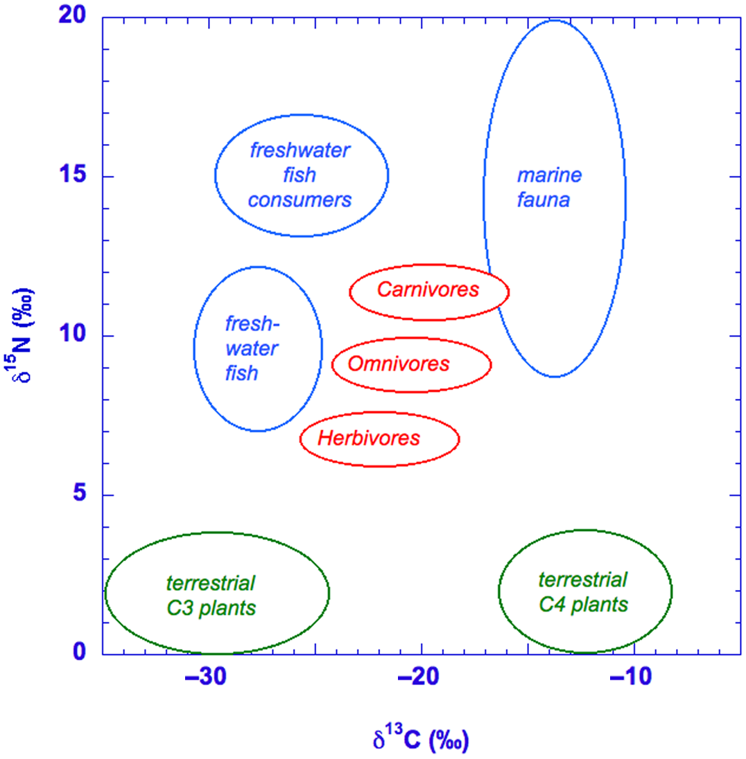
Figure 3 Schematic representation of (part of) the food web, indicating the relative ranges of δ13C and δ 15N values.
The dataset consists of data of terrestrial and aquatic organisms. For the latter, the 14C dates need correction for reservoir effects in order to derive absolute ages. This also applies to terrestrial organisms with a significant aquatic food subsistence. The latter is not simply 400 years (the general marine Holocene value) but can be riverine (or a mixture of both) since the Early Holocene landscape of the present North Sea region was a delta. The stable isotopes δ13C and δ15N are a necessary tool to quantify reservoir effects. The present tables consist for a major part of unpublished 14C, 13C, and 15N data, and can be used in the future to further zoom in on this question. In all figures and tables, the 14C ages (BP) are given instead of calibrated dates (calBP) to avoid reservoir effect ambiguities.
The data represents marine carnivores, terrestrial carnivores, omnivores (incl. humans), herbivores, and one bird species (Tables 1 and 2). The majority of the animal samples correspond to the Pleistocene. Indeed, many samples belong to typical Late Pleistocene mammoth steppe fauna, including woolly mammoth, cave lion, arctic fox, hyena, woolly rhinoceros, horse, giant deer, reindeer, and bison. In addition, the dataset includes 19 marine animals with a Pleistocene age, such as bowhead whale, common rorqual, beluga whale, grey whale, grey seal, harp seal, walrus, and great auk.
The rest of the samples correspond to the Holocene era: 61 animal skeletal remains, including 25 artifacts/worked items made of antler and bone. There is also a significant dataset of human bones. Here we will only use their average values of stable isotope ratios, for comparison with those of the fauna. For more details we refer to van der Plicht et al. (Reference van der Plicht, Amkreutz, Niekus, Peeters and Smit2016). Many finds come from a relatively limited number of areas from the North Sea, specifically locations that are frequently exploited by fishermen and that are suitable for sand extraction purposes. Indeed, about a third of the samples come from the important fishing areas Brown Bank (n = 53) and Eurogully (n = 43). Also, a large part (n = 38) comes from the Dutch province Zuid-Holland, in which many large sand suppletion projects took place in recent years (Maasvlakte, Zandmotor; see Figure 1).
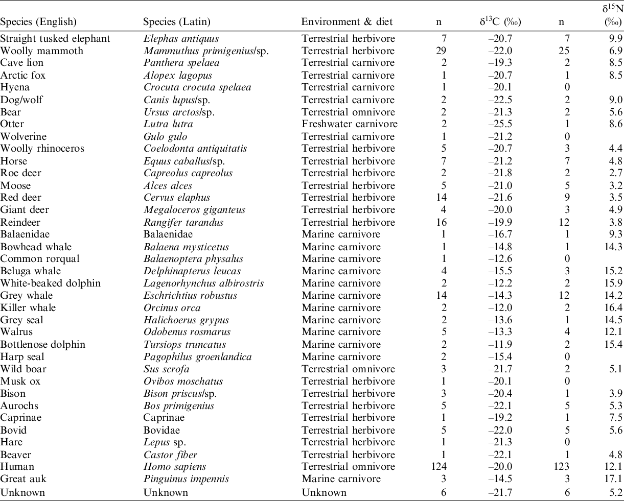
Table 3 (see Appendix) shows an overview summary of the analysed species, number of samples, class, environment (marine or terrestrial) and trophic level, with the (averaged) value of δ13C and δ15N. Figure 4 shows the mean δ13C and δ15N values for the samples, roughly ordered per trophic niche. In general, the isotope signals of most species fit into broad groups as shown in Figure 3. As expected, the marine carnivores show the highest δ13C and δ15N values. Their δ13C values range between –16.7 and –11.4 ‰, and the δ15N values between +9.3 and +17.7‰. The terrestrial herbivores show δ13C values ranging from –23.3 to –18.9‰. The δ15N values cover a large range of 9.9‰, the lowest being +1.7‰ and the highest δ15N value (+11.6‰) being higher than those of the terrestrial omnivorous animals and terrestrial carnivores in the current dataset.

Figure 4 Mean stable isotope (δ13C and δ15N) values with one sigma standard deviation for all animal samples, ordered per trophic level (herbivore, carnivore, omnivore) and habitat (marine, terrestrial). All samples are from mammals.
Apart from the humans, the terrestrial omnivores data fall within the range of these of terrestrial herbivores; δ13C values range between –22.3 and –20.3‰, and δ15N between +3.5 and +7.7‰. The humans show large ranges of both isotope values (see van der Plicht et al. Reference van der Plicht, Amkreutz, Niekus, Peeters and Smit2016). The terrestrial carnivores have δ13C and δ15N values between –25.6 and –19.2‰ and between +7.7 and +10.2‰, respectively. The dataset consists of two samples of a freshwater carnivore, an otter, with a δ13C value of –26.2‰ and –24.8‰, and a δ15N value of +8.6‰ (the δ15N of only one sample has been measured). These categories of trophic level/habitat are composed of a variety of species from different time periods. In the following, results of a number of species will be discussed in more detail. This selection is primarily based on the number of available samples per species.
The data for the Pleistocene samples are shown in Figure 5. As can be seen, the δ15N values of straight-tusked elephant (+7.5 to +11.6‰) and many of woolly mammoth (+5.0 to +9.1‰) exceed these of other herbivores. Relatively high δ15N values are commonly observed for woolly mammoths (e.g., Bocherens Reference Bocherens2003; Kuitems et al. Reference Kuitems, van Kolfschoten and van der Plicht2015a) and has also been observed for Middle-Pleistocene straight-tusked elephants from Germany (Kuitems et al. Reference Kuitems, van der Plicht, Drucker, van Kolfschoten, Palstra and Bocherens2015b). The current dataset also includes woolly mammoth samples with lower δ15N values. This has also been observed for Late-Glacial woolly mammoths in the Ukraine (Drucker et al. Reference Drucker, Bocherens and Péan2014), and has been associated with changing environments and/or climates and changes of niche occupation after the Last Glacial Maximum (LGM). Pre-LGM values of mammoths from Europe (including samples from the Ukraine) show higher δ15N values, ranging between 6.7‰ and 11.1‰ (Drucker et al. Reference Drucker, Bocherens and Péan2014). The current dataset of the North Sea contains only mammoth samples dating pre-LGM, the majority being older than the 14C background (>45,000 BP). The woolly mammoth samples with the lowest δ 15N values (between +5.0 and +6.0‰) are all older than 45,000 years BP.
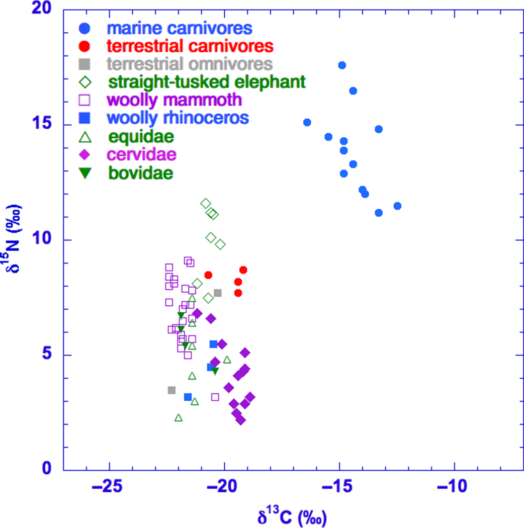
Figure 5 Stable isotope (δ13C and δ15N) values for Pleistocene mammal samples from the North Sea.
The δ13C values of woolly mammoths (–22.4 to –21.4‰) are rather negative compared to these of other herbivores, including straight-tusked elephants (–21.2 to –20.2‰). Also, this picture (woolly mammoths are depleted in δ13C compared to other herbivores) is known for other localities and has tentatively been linked to seasonally metabolism of stored fat (Bocherens Reference Bocherens2003; Szpak et al. Reference Szpak, Gröcke, Debruyne, MacPhee, Guthrie, Froese, Zazula, Patterson and Poinar2010).
All horses (n = 6) in this dataset originate from the (Late) Pleistocene. Their δ15N and δ13C values range from +2.3 to +6.4‰ and from –22.0 to –19.9‰, respectively. The general view of the horse diet is that it consists predominantly of grasses. However, dental wear studies on molars from Middle Pleistocene horses from Europe, with considerably low δ15N values, indicated that these specimens were mainly browsing (Rivals et al. Reference Rivals, Julien, Kuitems, van Kolfschoten, Serangeli, Bocherens, Drucker and Conard2015). The lower δ15N values have also been interpreted as the result of a browsing diet for these specimens (Kuitems et al. Reference Kuitems, van der Plicht, Drucker, van Kolfschoten, Palstra and Bocherens2015b), since usually browsers tend to have lower δ15N values than grazers (and lower δ13C values; e.g., Drucker et al. Reference Drucker, Hobson, Ouellet and Courtois2010). Another recent study on a Middle Pleistocene site from France (Richards et al. Reference Richards, Pellegrini, Niven, Nehlich, Dibble, Turq and McPherron2017) revealed that stable isotope values from horse dentine samples in a temporal sequence followed environmental and possibly climatic changes through time. Here, the lowest δ15N values (about +2 to +3‰) are linked to low temperatures. The lowest δ15N values of horse samples in the current dataset from the North Sea can either be caused by a specific diet (i.e., browsing) or low temperatures and/or high amounts of precipitation (i.e., affecting the δ15N values of plants they are feeding on), or by a combination of these factors.
Well-defined temporal changes in the distribution of δ13C and δ15N values have been observed for several species within North-western Europe, related to the climatic and environmental differences during the Late-Glacial and/or around the Pleistocene-Holocene boundary. These include changes in atmospheric CO2 concentrations (Richards and Hedges Reference Richards and Hedges2003; Stevens and Hedges Reference Stevens and Hedges2004), climatic variation on a local-scale including soil moisture conditions (Stevens and Hedges Reference Stevens and Hedges2004; Fox-Dobbs et al. Reference Fox-Dobbs, Leonard and Koch2008), and forest development after the LGM (Drucker et al. Reference Drucker, Bocherens and Billiou2003, Reference Drucker, Bidault, Hobson, Szuma and Bocherens2008), leading to depleted δ13C values in the Holocene.
Indeed, the Pleistocene-Holocene boundary is characterized by severe climatic and environmental changes for the area of the current North Sea. In general, the onset of the Holocene is characterized by wetter and warmer climatic circumstances, sea level rise and forest development. The current stable isotope record for the North Sea does not allow for statements on temporal trends: none of the species is represented (in appropriate numbers) in both Pleistocene and Holocene. Moreover, in general, samples from the last part of the Late-Pleistocene, i.e., the LGM and the Late Glacial, are lacking (see Tables 1 and 2 and Figure 2).
In contrast to the characteristic Pleistocene “mammoth steppe fauna,” generally thriving in open landscapes, the Holocene samples represent specimens from temperate species and forest dwellers. This is illustrated by the North Sea samples of cervids: Pleistocene samples are chiefly from reindeer, and consists further of giant deer and moose, whereas the Holocene samples of cervids predominantly consists of red deer, and further include moose and roe deer. As shown in Figure 6, the δ13C values of samples from Holocene cervids (n = 22, average = –21.7‰) are considerably more negative than those of the Pleistocene cervids (n = 20, average = –19.7‰).

Figure 6 Stable isotope δ13C values for samples of cervids from the North Sea through time.
This difference can partly be ascribed to the changed δ13C values of plants caused by the climatic shift from the Pleistocene to the Holocene. Moreover, this difference can be explained by dissimilarities between the species, such as niche occupation, physiology and dietary composition. For instance, in general the diet of reindeer consists for a significant part of lichens, which commonly yield higher δ13C values than vascular plants (Ben-David et al. Reference Ben-David, Shochat and Adams2001; Drucker et al. Reference Drucker, Bocherens and Billiou2003).
Due to the sea level rise, samples of marine mammals recur in the Holocene record. Considering the marine bone samples, a number of the walruses (Odobenus rosmarus) has a low nitrogen isotope ratio (n = 4; average = +12.1‰) compared to most other marine mammals (average = +14.5‰). This might be ascribed to the feeding on food sources of a low trophic level, such as clams and other molluscs (Dehn et al. Reference Dehn, Sheffield, Follmann, Duffy, Thomas and O’Hara2007).
The freshwater species is only represented by two samples from a Holocene otter. Also, the stable isotopes of the Holocene dog/wolf (Canis sp.; GrA-24209) show mainly a freshwater signal (Figure 7). This is not surprising, since the Holocene dog lived together with humans, as is known from other sites in Northwestern Europe (e.g., Noe-Nygaard Reference Noe-Nygaard1983, Reference Noe-Nygaard1988; Schulting and Richards Reference Schulting and Richards2002; Fischer et al. Reference Fischer, Olsen, Richards, Heinemeier, Sveinbjornsdottir and Bennike2007). In general, freshwater fish was an important part of the diet of Mesolithic humans in this area (see next paragraph). Their dogs might have consumed the “rest” of the human meal (Noe-Nygaard Reference Noe-Nygaard1983), causing a freshwater signal. Besides numerous samples from human skeletal remains, abundant finds of stone tools indicate the presence of Mesolithic hominins in the North Sea area.
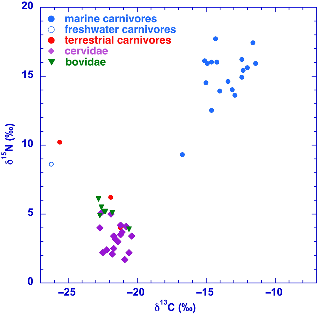
Figure 7 Stable isotope (δ13C and δ15N) values for Holocene animal samples from the North Sea.
Indeed, during the Mesolithic the higher areas in the coastal landscape of the North Sea, such as river dunes were inhabited. A well-known example is the archaeological site Hardinxveld-Giessendam De Bruin (Louwe Kooijmans et al. Reference Louwe Kooijmans, Ball, Brinkkemper, van Wijngaarden, Bakels, Beerenhout and Hänninen2001). Among the faunal remains that were submitted for radiocarbon dating are numerous pieces of worked bone and antler, including artifacts. These comprise long bones of bovids, equids, and cervids, and antler predominantly of red deer. The bone material from six of such objects could not be identified at species level. These are plotted as “unknown.” The δ13C and δ15N values fall within the ranges of terrestrial herbivores. This is not surprising as artifacts were usually made from cervid bone.
CONCLUSIONS
The North Sea region was dry land during the last glacial period and was inhabited by a rich fauna. This yields large quantities of fossil bones recovered from the present seabed. Over the years, more than 200 animal bones are dated by 14C, including a significant amount from extinct species. These were dredged up from the sea bottom or are found on the beach or on sand suppleted areas. Since the finds are recovered without a clear context, the dates yield crucial information for reconstructions of the past environment in a multidisciplinary setting.
We discuss here the available dates and show that most fossil bones provide important information on palaeontology, palaeoecology, landscape, and archaeology for this unique heritage site. The stable isotope ratios δ13C and δ15N of the dated bones illustrate that a collection of stray finds without context nevertheless can lead to inference of past environments in a multidisciplinary approach. For most of the animal remains from the North Sea, this is the first time that the stable isotope values are discussed. This consists of information on both extinct and extant terrestrial and aquatic species. The extinct species include straight-tusked elephant, woolly mammoth, woolly rhinoceros, and cave lion.
As a heritage site, the North Sea area has been archaeologically and palaeonotlogically extensively explored by both classic methods and modern techniques. Radiocarbon dates and stable isotope data add valuable information on environmental conditions and dietary habits in this area through time.
APPENDIX
Table 1 Data for North Sea fossil animal bones, selected for Late Pleistocene and for infinite 14C age (>45,000 BP). The table contains a column indicating the quality aspect of the measurement, wherein “a” means accepted, “1” accepted but not all criteria known, “2” not all criteria met but accepted, “3” accepted but only C isotopes measured. The calibrated dates are shown at 95% confidence level (“low” to “high”).

Table 2 Data for North Sea fossil animal bones, selected for Holocene age. The table contains a column indicating the quality aspect of the measurement, wherein “a” means accepted, “1” accepted but not all criteria known, “2” not all criteria met but accepted, “3” accepted but only C isotopes measured. The calibrated dates are shown at 95% confidence level (“low” to “high”).
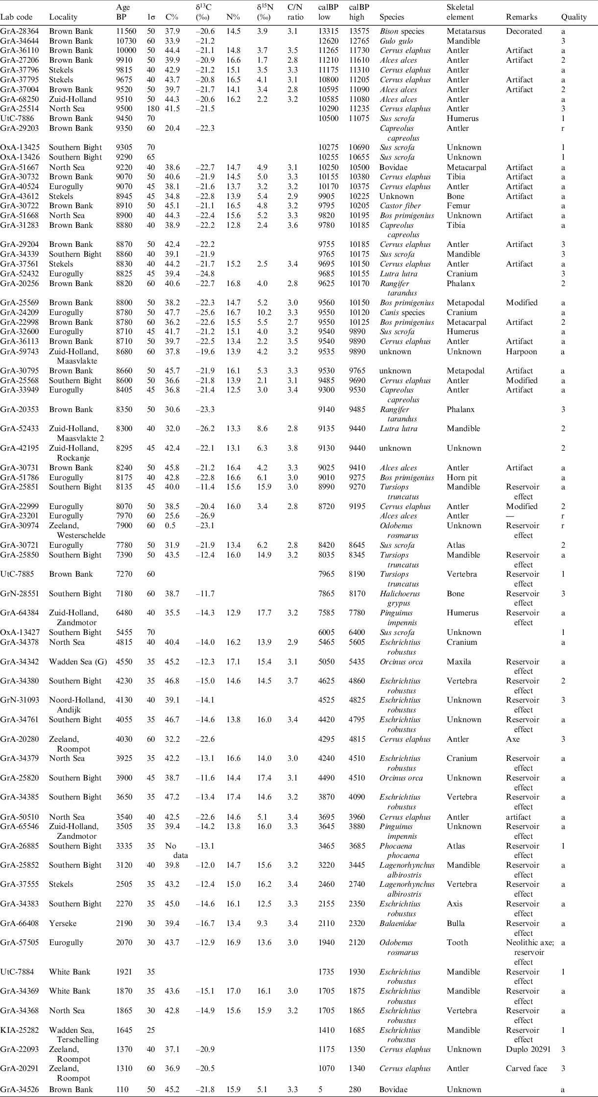
Table 3 Overview of analyzed species, environment and average values of the stable isotope ratios δ13C and δ15N.


 Open access