


INTRODUCTION
The Coastal Oyashio (CO) and Oyashio regions along the southwestern edge of the western subarctic gyre in the North Pacific Ocean (Fig. 1) are characterized by high macronutrient concentrations, primary production, and mesozooplankton biomass (Sakurai, Reference Sakurai2007; Ikeda et al., Reference Ikeda, Shiga and Yamaguchi2008). These regions provide important nursery grounds for a wide range of commercially important marine fishery resources, such as Japanese sardine and Japanese anchovy (Sakurai, Reference Sakurai2007). The CO water flows on the continental shelf along the Pacific coast off southeastern Hokkaido, extends westward, partly intrudes the Funka Bay through Hidaka Bay, and reaches the vicinity of the Sanriku coast during winter–spring (e.g., Hanawa and Mitsudera, Reference Hanawa and Mitsudera1986; Fig. 1). The CO transports very cold and low-salinity water (typically with temperature <2°C and salinity <33) that originates in the Okhotsk Sea. In addition, the CO water exhibits much higher concentrations of dissolved iron (2.8 nM) than Oyashio water near the sea surface (~0.2 nM) during the pre-bloom period (Nishioka et al., Reference Nishioka, Ono, Saito, Sakaoka and Yoshimura2011), significantly contributing to the occurrence of a ‘massive spring bloom,’ typically with very high chlorophyll a (Chl-a) concentrations exceeding 5 mg m−3 (Fig. 1; Isada et al., Reference Isada, Hattori-Saito, Saito, Kondo, Nishioka, Kuma, Hattori, McKay and Suzuki2019; Kuroda et al., Reference Kuroda, Toya, Watanabe, Nishioka, Hasegawa, Taniuchi and Kuwata2019). Therefore, the transport of CO water with high concentrations of dissolved iron plays a major role in regulating the generation and spatial extent of massive spring blooms over the Oyashio area (Kuroda et al., Reference Kuroda, Toya, Watanabe, Nishioka, Hasegawa, Taniuchi and Kuwata2019).

Figure 1. Study area around Hokkaido, Japan. (a) main current systems, coring sites, sediment-trap study site, and observational stations. Closed circle denotes coring site T3 (piston core T3, multi-core T3 MC4-1); open circles represent previous coring sites (SK-2: Sagawa et al., Reference Sagawa, Kuwae, Tsuruoka, Nakamura, Ikehara and Murayama2014; CH84-14: Crusius et al., Reference Crusius, Pedersen, Kienast, Keigwin and Labeyrie2004; GH01-1011: Itaki and Ikehara, Reference Itaki and Ikehara2004); open triangle is sediment trap study site MD01-2409 of Kawahata et al. (Reference Kawahata, Minoshima, Ishizaki, Yamaoka, Gupta, Nagao and Kuroyanagi2009); open star is observational station E16. (b, c) Study area in relation to surrounding areas of the Pacific showing mean surface Chl-a concentrations in March–April for 2003–2020 as measured by the Moderate Resolution Imaging Spectroradiometer (MODIS) aboard the Aqua satellite from the NASA Goddard Space Flight Center, Ocean Ecology Laboratory, Ocean Biology Processing Group (NASA OB.DAAC, Greenbelt, MD, USA. doi: 10.5067/AQUA/MODIS/L3B/CHL/2018, accessed on 26/03/2021); (c) is enlarged map of the area in the white rectangle in (b). In (b), open circles denote coring sites T3 (piston core T3, multi-core T3 MC4-1), LV28-4-4 (Lembke-Jene et al., Reference Lembke-Jene, Tiedemann, Nürnberg, Gong and Lohmann2018), and PC06 (Minoshima et al., Reference Minoshima, Kawahata and Ikehara2007); DSW: dense shelf water, ESC: Eastern Sakhalin current, OSIW: Okhotsk Sea intermediate water, CO: Coastal Oyashio, OY: Oyahio, EKC: East Kamchatka Current, WSG: Western Subarctic Gyre, K-O: Kuroshio-Oyashio transition, KR: Kuroshio, KE: Kuroshio Extension.
The CO is a coastal boundary current that originates from the East Sakhalin Current in the Okhotsk Sea (Fig. 1); the CO on the Pacific shelf can be regarded as a downward extension of the East Sakhalin Current on the shelf from the Okhotsk Sea (Isoda et al., Reference Isoda, Kuroda, Myousho and Honda2003; Kuroda et al., Reference Kuroda, Toya, Watanabe, Nishioka, Hasegawa, Taniuchi and Kuwata2019). The East Sakhalin Current is driven by wind stress induced at the sea surface along the Sakhalin coast in the Okhotsk Sea, and is primarily controlled by the dynamics of the arrested topographic waves (Csanady, Reference Csanady1978). The dynamics of the CO are somewhat modified on the Pacific shelf; a shelf-break frontal jet is dominant on the shelf along southeastern Hokkaido (Sakamoto et al., Reference Sakamoto, Tsujino, Nishikawa, Nakano and Motoi2010), and a coupled remote–local arrested topographic wave is dominant on the southwestern shelf (Kuroda et al., Reference Kuroda, Isoda, Takeoka and Honda2006).
It is interesting to note that there was a step-function-like regime shift of sea surface temperature (SST) and the Western Pacific (WP) index in 2015/2016 (https://www.cpc.ncep.noaa.gov/data/teledoc/wp_ts.shtml, accessed December 2, 2021), which corresponded to an abrupt weakening of the East Sakhalin Current (Supplementary Figure 1). Concomitantly, satellite-based chlorophyll concentrations decreased during spring in a wide area, including downstream of the CO (Hidaka Bay and Funka Bay), Oyashio, and the Kuroshio–Oyashio transition, except for the Oyashio off southeastern Hokkaido, in which the concentrations increased (Fig. 2). Therefore, CO dynamics potentially cause decadal-scale changes in biological production in the western North Pacific through large-scale atmospheric forcing associated with decadal climate variability.
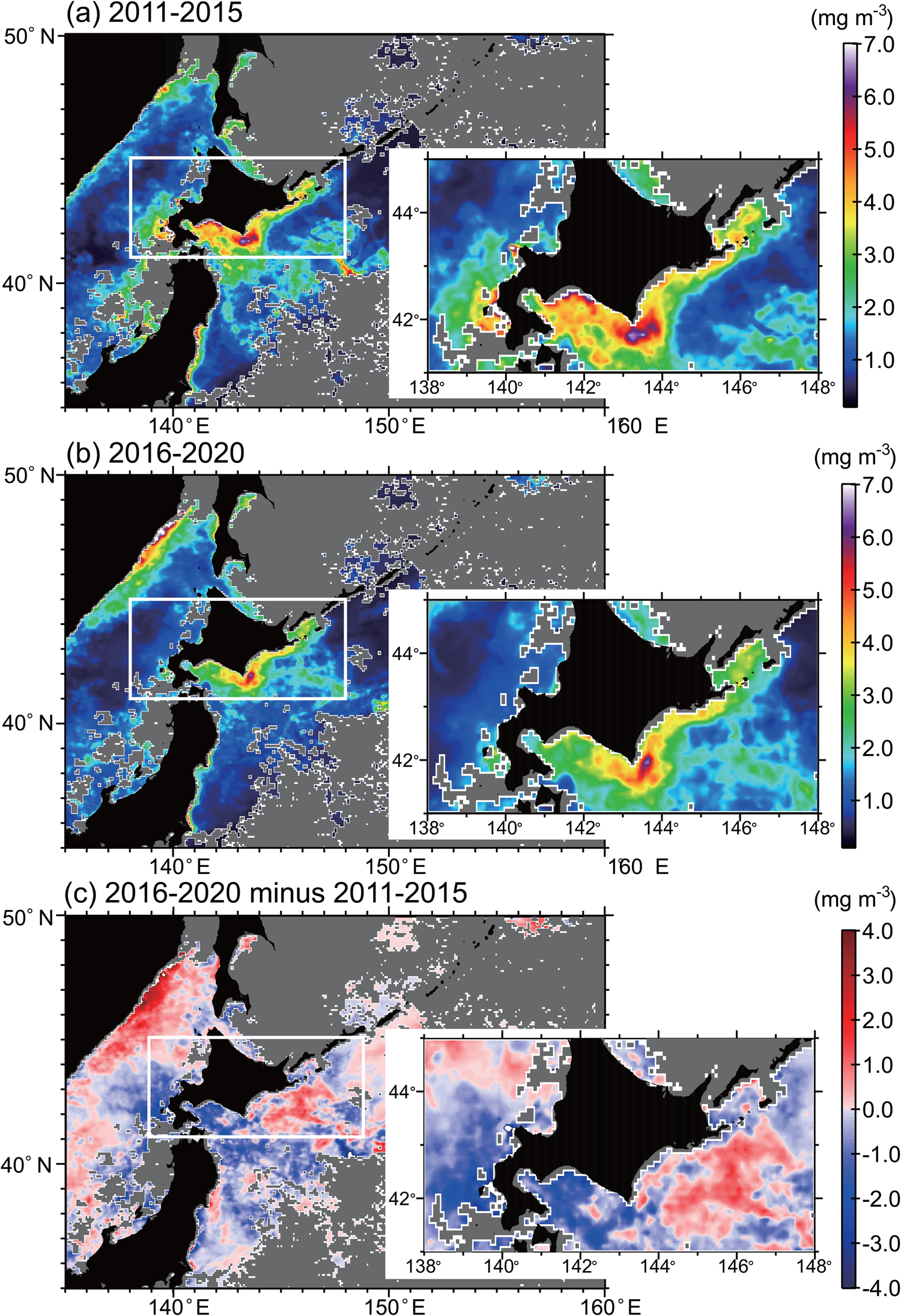
Figure 2. Satellite-based mean chlorophyll concentrations in March to April during (a) 2011–2015, (b) 2016–2020, and (c) difference (b-a) between mean chlorophyll concentrations. Study site T3 is within Hidaka Bay (white rectangle), and it shifted to a low chlorophyll and high SST regime after 2015/2016 when volume transport of the Coastal Oyashio weakened simultaneously (Supplementary Figure 1). Gray areas denote missing values due to cloud cover.
Previous paleoceanographic studies conducted in the western North Pacific have documented changes in biological productivity. The total organic carbon (TOC) and biogenic opal concentrations in the Oyashio (core site PC6, Minoshima et al., Reference Minoshima, Kawahata and Ikehara2007), CO (core site CH84-14, Crusius et al., Reference Crusius, Pedersen, Kienast, Keigwin and Labeyrie2004), and Okhotsk Sea showed millennial-scale variations in primary productivity during the Holocene. However, the time resolutions of previously obtained records were not fine enough to detect centennial-scale variability in productivity. With respect to higher trophic-level organisms, decadal-to-centennial variability in Japanese sardine and Japanese anchovy migrating in the western North Pacific was revealed in fish-scale records from Beppu Bay, southwest Japan, near the main spawning grounds for these species (Kuwae et al., Reference Kuwae, Yamamoto, Sagawa, Ikehara, Irino, Takemura, Takeoka and Sugimoto2017). The Japanese sardine record shows a decreasing trend in the maximum values of decadal-to-centennial fluctuations. Although other diverse fish species inhabit the area, to date there have been no paleoceanographic records of zooplankton, which are the main prey organisms for these fish. Although several well-known marine paleofish productivity reconstructions have been created for large marine ecosystems (e.g., Gulf of Alaska, off Peru, Chile, California, and South Africa) (Baumgartner et al., Reference Baumgartner, Soutar and Ferreira-Bartrina1992; Finney et al., Reference Finney, Gregory-Eaves, Douglas and Smol2002; Struck et al., Reference Struck, Altenbach, Emeis, Alheit, Eichner and Schneider2002; Valdés et al., Reference Valdés, Ortlieb, Gutierrez, Marinovic, Vargas and Sifeddine2008; Gutiérrez et al., Reference Gutiérrez, Sifeddine, Field, Ortlieb, Vargas, Chávez and Velazco2009; Salvatteci et al., Reference Salvatteci, Gutierrez, Field, Sifeddine, Ortlieb, Caquineau, Baumgartner, Ferreira and Bertrand2019), the long-term dynamics of zooplankton productivity and even bottom-up or top-down control of zooplankton production in the food chain remain unclear. Therefore, the dynamics of marine food chains from primary producers to fish on centennial and longer timescales have rarely been addressed.
Here, we reconstruct high-resolution (mean: 34-year intervals) records of algal and zooplankton productivity using Late Holocene sediment core samples from Hidaka Bay, located within the CO system (Kuroda et al., Reference Kuroda, Toya, Kakehi, Setou, Chen and Guo2020). These sediments allow us to address the following five questions: 1) can sedimentary chlorophyll a and its derivatives (Chl-a) and steryl chlorin esters (SCEs) be used as proxies for spring primary and secondary productivity, respectively? 2) Are there long-term trends and centennial-scale variability in biological production? 3) Is there evidence for bottom-up effects on zooplankton productivity? 4) Do long-term trends and centennial variability in primary and secondary productivity in the records reflect the response to changes in the frequency of CO intrusion into Hidaka Bay? CO water contains diatom species inhabiting sea ice that is transported by the East Sakhalin Current. Sea-ice-associated diatoms are a powerful proxy for detecting CO intrusions in Hidaka Bay. By analyzing fossil diatom assemblages in the sediments, including sea-ice-associated diatoms, the influence of CO and its iron supply on productivity in the bay could be assessed. 5) Is zooplankton productivity responding to iron supply from the CO associated with the abundance of Japanese sardine in the western North Pacific?
STUDY SITE AND MARINE SETTING
The study area is located on the slope off the southern part of Hokkaido, Japan (Fig. 1, site T3, water depth: 607 m). The sediments are generally composed of a mixture of fine-grained clastic sediments and biogenic materials, predominately opal. Occasional disruptions of pelagic sedimentation processes in this tectonically active region might be associated with tsunami, volcanic, and earthquake events, and these disruptions are recognizable in the core stratigraphy. Giant earthquakes are posited to have occurred at an average recurrence interval of ca. 400 years, with variations ranging between 100 years and 800 years (Sawai et al., Reference Sawai, Kamataki, Shishikura, Nasu, Okamura, Satake, Thomson, Matsumoto, Fujii and Komatsubara2009; Ishizawa et al., Reference Ishizawa, Goto, Yokoyama, Miyairi, Sawada, Nishimura and Sugawara2017). In the coastal area near the T3 site, there are two tsunami layers in the coastal lowlands of southern Hokkaido, corresponding to those formed in the seventeenth and eighteenth centuries (Takashimizu et al., Reference Takashimizu, Nagai, Okamura and Nishimura2013).
Hidaka Bay is well suited as a study site for these questions because it is in the westernmost part of CO near the Hokkaido coast (Supplementary Figure 2), where spring biological production responds to the frequency of CO water westward intrusions (Fig. 2; Supplementary Materials 1).
METHODS
Sediment cores
A piston core (T3; inner diameter of pipe: 75 mm) and one of the multi-cores (T3 MC4-1; inside diameter of pipe: 82 mm) were sampled during the R/V Tansei-Maru KT-10-5 cruise (April 21, 2010) at 42°14.083′N, 141°34.987′E, at a water depth of 607 m off the southern coast of Hokkaido, Japan (Fig. 1). The piston core T3 (690.1 cm in length, Fig. 3; Supplementary Figure 3) was sectioned every 1 m (sections 4 to 10, Supplementary Table 1), split in half, and sliced at intervals of 1 cm (sections 4 to 5) or 2 cm (sections 6 to 10). For geochemical and diatom analyses, we used the sliced samples at an interval of 2 cm for T3 (mean time resolution: 46 years) and 1 cm for T3 MC4-1 (mean time resolution: 20 years), except for high-density event layers. We determined the boundaries of the event layers from CT images, which were confirmed by anomalously higher values of dry bulk density relative to the background trend (Fig. 3).
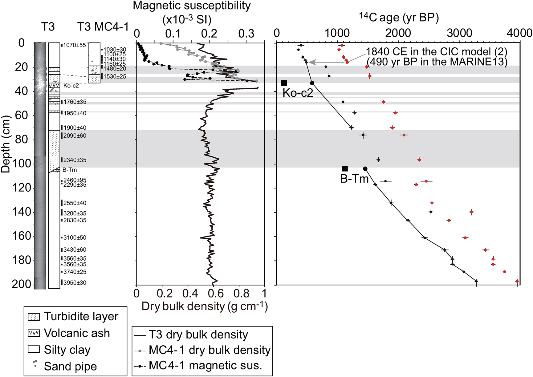
Figure 3. CT images, core lithology, dry bulk density, magnetic susceptibility, and 14C ages for the upper ~200 cm of cores T3 and T3 MC4-1. Data are shown for 0–205 cm in core T3 and 0–33 cm in core T3 MC4-1. Solid rectangles with ages and errors right side of lithology denote 14C sample horizons and 14C yr BP. The right panel shows raw 14C ages (small red circles) and those corrected by a ΔR value of 670 years (small black circles) (see Supplementary Materials 1). Horizontal shaded bands denote levels of turbidite layers. Large solid squares and circles denote 14C ages of tephra (Ko-c2: Yamada, Reference Yamada1958; B-Tm: Machida et al., Reference Machida, Arai and Moriwaki1981) based on Intcal13 and MARINE13 dataset, respectively. Solid lines denote those connected by 14C data plots from the ‘normal’ sediments and age-controls of tephra used for Bayesian age modeling. (For interpretation of references to color in this figure legend, the reader is referred to the web version of this article.)
Identification of tephra samples was based on petrographic properties and major element compositions of volcanic glasses. The major element compositions of the tephra glasses were determined using an energy-dispersive X-ray spectrometer (JEOL JSM-5310).
‘Event-free’ composite core depth
For chronological analysis, we developed a composite core depth scale by correlating the piston and multi-cores at the turbidite layers (28–33 cm depth in core for T3 MC4-1 and 26.0–33.1 cm for T3; Supplementary Materials 1). The composite core depth (ccd) we used was based on core T3 MC4-1 above the bottom of the turbidite layer (raw depth of 33 cm in MC4-1) and core T3 below the turbidite layer (raw depth of 33 cm in T3) (Supplementary Table 1). Then, the ‘event-free’ composite core depth (efd) was determined by subtracting the thicknesses of all turbidite and volcanic ash layers from cores T3 MC4-1 and T3 (Supplementary Table 1).
Dating
Core chronology was based on 210Pb dating (Appleby and Oldfield, Reference Appleby and Oldfield1978) for the upper portion of core T3 MC4-1, and on tephra eruption dates and 14C dating for the remaining core. Samples for the 137Cs, 210Pb, and 214Pb analyses were collected at intervals of 1 cm to a depth of 24 cm in T3 MC4-1. The radioactivity was determined by gamma counting using a Ge-detector (GWL–90-15–S, EG&G ORTEC, USA) equipped with a multichannel analyzer (MCA7700, SEIKO EG&G, Tokyo, Japan) at the Research Institute for Humanity and Nature in Japan. Dried samples were sealed in holders for a month to allow 222Rn and its short-lived daughters (214Pb) to equilibrate. The activity of the supported 210Pb was estimated by measuring the activity of 214Pb, whereas that of 210Pbexcess was determined using the difference between the total and supported 210Pb:
Regarding the chronology of the upper sediments, we compared several age models constructed based on the constant initial concentration (CIC) model (Robbins and Edgington, Reference Robbins and Edgington1975), the 137Cs fallout-based model, and the constant rate of supply (CRS) method of 210Pb dating (Appleby and Oldfield, Reference Appleby and Oldfield1978). Two CIC models were produced to assess the bioturbation effects on excess 210Pb profiles (as described later): model 1, where two different regression lines in the upper and lower layers were applied to the CIC model, and model 2, where only the regression line in the lower layer was applied to the CIC model, assumed as the bioturbation active layer in the upper layer and below its depth, which is reliable for estimating the sedimentation rate.
The age-depth model below the zone of excess 210Pb activity for both cores T3 MC4-1 and T3 was constructed from benthic foraminiferal 14C ages. The measurements of accelerator mass spectrometry (AMS) 14C ages were performed for mixed benthic foraminifera by the National Ocean Sciences Accelerator Mass Spectrometer (NOSAMS) facility at Woods Hole Oceanographic Institute, USA. Stable carbon isotope values for the correction of isotopic fractionation were measured during AMS sample preparation or processing by NOSAMS. Age models were generated using OxCal v.4.3 (Bronk Ramsey, Reference Bronk Ramsey2009), where Bayesian statistical methods for calibration of 14C data and the MARINE13 calibration set (Reimer et al., Reference Reimer, Bard, Bayliss, Beck, Blackwell, Bronk Ramsey and Buck2013) were used. The 14C-based age-depth model was constructed using the Bayesian approach in terms of calibration in conjunction with the P-sequence deposition model (assuming that the deposition is a Poisson process) installed in OxCal 4.3 (Bronk Ramsey, Reference Bronk Ramsey2008) together with ΔR values of 670 ± 50 yr (Supplementary Materials 1).
Biogenic opal content
The biogenic opal (bio-opal) content was determined using a slightly modified method based on that developed by Mortlock and Froelich (Reference Mortlock and Froelich1989). The sediment samples were crushed into fine powder after being dried at 50°C for 24 h. Solutions of 30% HCl and 8% H2O2 were added to 30 mg of the sample in a polypropylene centrifuge tube to remove calcium carbonates and organic materials. The bio-opal contents were determined through extraction using 10 ml of a 2 M Na2CO3 solution at 83°C for 2 h, followed by molybdate-yellow spectrophotometry with a Shimazu UV Mini-1240v spectrophotometer in Center for Marine Environmental Studies, Ehime University. Residues of the selected samples were examined under an optical microscope to verify the complete dissolution of the siliceous microskeletons. The relative standard deviation analysis of bio-opal was 2% in the replicate analyses. All values were reported as 10% hydrated opal (SiO2 • 0.4 H2O) by using a multiplier of 2.396 on Si.
Elemental TOC and TN, organic matter δ13C, and sedimentary δ15N
Acid-washed (1 M HCl) samples were combusted in a Costech 4010 HCNS elemental analyzer at the Stable Isotope Laboratory at Idaho State University to determine the TOC and total nitrogen (TN) concentrations. The analyzer was coupled with a Finnigan Deltaplus Advantage isotope ratio mass spectrometer at the Stable Isotope Laboratory at Idaho State University for δ13C and δ15N measurements. All isotope values were reported in permil units (‰) according to the following relation:

where X is the element of interest and R is the measured isotopic ratio. All carbon isotope measurements are relative to the Vienna Pee Dee Belemnite standard and all nitrogen measurements are relative to atmospheric nitrogen. The molar ratios of TN:TOC (C/N) were calculated by following Perdue and Koprivnjak (Reference Perdue and Koprivnjak2007). Replicate measurements of internal standards conducted along with TOC and TN yielded 4.4% and 6.9% coefficients of variation, respectively, whereas those of internal δ13C and δ15N standards yielded 1σ standard deviations of 0.19‰ and 0.20‰.
To reconstruct carbon-based marine biological productivity, we estimated the marine-derived organic carbon (OCmarine) fraction using both a δ13C-based two-source mixing model (Gordon and Goñi, Reference Gordon and Goñi2003) and an atomic C/N-based model (Perdue and Koprivnjak, Reference Perdue and Koprivnjak2007; Supplementary Materials 1). In the shelf and slope areas along southeast Hokkaido located in the upstream CO area, the δ13C in the surface sediments tends to approach lower values in samples taken closer to the coast. Usui et al. (Reference Usui, Nagao, Yamamoto, Suzuki, Kudo, Montani, Noda and Masao Minagawa2006) demonstrated that the δ13C (C/N) variations in the surface sediments can be explained by the mixing ratios of marine- and terrestrial-origin organic matter with end-member values of −21.0 (8.4) and −26.9 (16.4), respectively. We applied these end-member values to estimate the contributions of OCmarine to TOC in the T3 core samples.
Algal pigments and SCEs
Concentrations of fossil pigments were quantified using high-performance liquid chromatography (HPLC). Frozen sediments were placed in 10 mL glass vials. HPLC-grade acetone was added (3 mL), and the pigments were extracted at 0°C during agitation in an ultrasonic bath (Tani et al., Reference Tani, Matsumoto, Soma, Soma, Hashimoto and Kawai2009a, Reference Tani, Nara, Soma, Soma, Itoh, Matsumoto, Tanaka and Kawaib). The extracts were collected after centrifugation at 2000 rpm for 5 min. These procedures were repeated at least three times for each sample until the supernatant became completely colorless. The combined extract was evaporated to dryness under N2, dissolved in 3 mL diethyl ether, and washed with an aqueous solution of NaCl (1 M). After evaporating the ether phase to dryness under N2, the residue was dissolved in 200–500 μL of acetone together with an internal standard, mesoporphyrin IX dimethyl ester (Sigma Chemical Company, USA), and analyzed by HPLC (LC-10CE, Shimadzu, Kyoto, Japan) using a photodiode array detector (SPD-M10AVP, Shimadzu, Kyoto, Japan). A Wakopack Navi C30-5 reverse-phase column (4.6 mm diameter, 250 mm length; Wako Pure Chemical Industries, Ltd., Japan) was used for separation. The mobile-phase solvent A was a mixture of acetonitrile and water (90:10 v/v), whereas solvent B was 100% ethyl acetate. A linear gradient from 100% A to 100% B over 40 min was followed by an isocratic hold for 10 min at 100% B. The flow rate was 1.0 mL min–1.
Pigments were identified based on retention times, absorption spectra of standard samples, and absorption coefficients. Because the SCE standards were not available, we identified them based on data from the literature (King and Repeta, Reference King and Repeta1991; Harradine et al., Reference Harradine, Harris, Head, Harris and Maxwell1996) and from previous analysis of sterols in hydrolyzed SCEs using HPLC-MS and GC-MS (Soma et al., Reference Soma, Itoh, Tani and Soma2005, Reference Soma, Tani, Soma, Mitake, Kurihara, Hashomoto, Watanabe and Nakamura2007). The pigments analyzed in this study were chlorophyll a (a major photosynthetic pigment ubiquitous in all taxonomic algae), its derivatives, and SCEs. In this paper, the sum of chlorophyll a and its transformation products (pheophytin a, pyropheophytin a, and pheophorbide a) is designated as Chl-a.
To detect post-depositional degradation of pigments, we used the chlorophyll a/pheophytin a ratio, which is an indicator of post-depositional pigment degradation because the labile precursor, Chl-a, is compared to the chemically stable product, pheophytin a (Leavitt and Hodgson, Reference Leavitt, Smol, Birks and Last2001).
Diatom assemblage analysis
The composition of diatom species in ocean sediments is widely used for paleoceanographic reconstructions of the dominance of water masses (Ren et al., Reference Ren, Gersonde, Esper and Sancetta2014). A distribution map of the relative abundance of diatom species in the surface sediments in the North Pacific shows that the East Sakhalin Current along Sakhalin and Hokkaido in the Okhotsk Sea is characterized by a high relative abundance of sea-ice-associated species, Bacterosira bathyomphala, Fragilariopsis oceanica, and Fragilariopsis cylindrus (Ren et al., Reference Ren, Gersonde, Esper and Sancetta2014), indicating that the sum of percentages of these species is a proxy for this water, and may trace intermittent intrusions of dissolved iron-replete CO water into Hidaka Bay.
For diatom assemblage analysis, 43 samples were obtained from the upper portion of cores T3 and T3 MC4-1. Freeze-dried samples weighing ~6 mg to ~100 mg depending on the diatom content were cleaned using solutions of 15% hydrogen peroxide and sodium hexametaphosphate. After the chemical reaction, clay minerals were removed and the solution was rinsed out through repeated decantation. The volume of the sample liquid was adjusted to 25 mL, then 1 mL of the well-mixed liquid was transferred onto a cover slip. The sample liquid present on the cover slip was gently dried. The cover slip with the sample on the surface was mounted on a microslide glass with Mountmedia® of Wako Pure Chemical Industries, Ltd. (refractive index ≥ 1.50). Under a light microscope with ×1000 magnification using immersion oil, more than 400 diatom valves in each prepared microslide were counted at the species or genus level.
Mass accumulation rates of biogeochemical properties
To obtain burial rates of biogeochemicals and to consider the dilution effects of clastic materials on the concentrations, mass accumulation rates (MARs; g cm−2 yr−1) for the upper layer (0–21 cm in composite core depth; ccd) were calculated using the following equation:

where C is the concentration of a property (g g−1 dry sediment) and SAR is the sediment mass accumulation rate (g dry sediment cm−2 yr−1), which is estimated from the CRS or CIC method of 210Pb dating. For the layers below 21 cm in ccd, MAR was calculated using the following equation:

where DBD is the dry bulk density (g dry sediment cm−3) and SR is the sedimentation rate (cm yr−1), which was estimated from 14C Bayesian statistical method-based dating (Supplementary Materials 1).
Mineral compositions
To obtain dilution effects of terrestrial materials on concentrations in biogeochemical proxies, mineralogical analysis was conducted using the random powder X-ray diffraction (XRD) method using an X-ray diffractometer equipped with a CuKa tube and monochromator (MX-Labo, Bruker AXS, Mac Science, Kanagawa, Japan) in the Faculty of Environmental Earth Science, Hokkaido University. Tube voltage was 40 kV, current was 20 mA, and the divergence, scattering, and receiving slits were 1°, 1°, and 0.15 mm, respectively. Freeze-dried powdered sediment samples were mounted on glass holders and x-rayed from 2°–40° 2θ. Scanning speed was 4° 2θ/min and the data sampling step was 0.02° 2θ. The diffractograms were processed using MacDiff v. 4.2.5 software (Petschicks, Reference Petschicks2021) for profile smoothing and background calculation. We report intensity (cps).
Principal component analysis
Principal component analysis (PCA) was used to identify primary factors influencing the variations in the biogeochemical parameters (bio-opal, Chl-a, chlorophyll a/pheophytin a, chlorophyll a/Chl-a, SCEs, δ13C, δ15N, TOC, TN, and C/N) and dry bulk density. We used data below 6.5 cm in ccd (before AD 1960, n = 65) to avoid any complication caused by early diagenesis of organic matter. Additionally, we performed PCA using biogeochemical parameters and diatom species to detect the leading mode of variability in productivity related to diatom-inferred water-mass dominance. We also performed PCA for mineral compositions, concentrations of bio-opal, Chl-a, and SCEs, dry bulk density, and sedimentation rates to determine minor or major effects of dilution of clastic materials on opal concentrations. PCA computations were conducted on centered and standardized data using CANOCO for Windows 4.5 (ter Braak and Šmilauer, Reference ter Braak and Šmilauer2002).
RESULTS
Tephra
A comparison of the data obtained with that of standard volcanic glasses (Nakamura, Reference Nakamura2016) indicates that the upper volcanic ash layer of core T3 was determined to be Ko-c2 (Yamada, Reference Yamada1958; Katsui et al., Reference Katsui, Suzuki, Soya and Yoshihisa1989; Supplementary Figure 4), which erupted from Mt. Komaga-Take, south Hokkadido, Japan. The 106-cm-deep tephra layer was determined to be the Baegdusan–Tomakomai tephra (B-Tm; Machida et al., Reference Machida, Arai and Moriwaki1981; Supplementary Figure 4), which erupted from the Baegdusan [Chang-baishan] caldera at the border between China and North Korea. The eruption ages of the Ko-c2 and B-Tm tephra were reported to be within AD 1694 (Furukawa et al., Reference Furukawa, Yoshimoto and Yamagata1997), and AD 946 in dendrochronological studies conducted using the AD 774–775 14C spike (Hakozaki et al., Reference Hakozaki, Miyake, Nakamura, Kimura, Masuda and Okuno2018), respectively.
Dating of the surface layer
The vertical profile of excess 210Pb in core T3 MC4-1 did not show a simple exponentially decreasing trend with respect to depth (Supplementary Figure 5). The slope of the excess 210Pb was steeper at levels below 17 cm than at higher levels. We produced two CIC-based age-depth models: CIC model 1, which was obtained using two different regression lines in the upper and lower layers, and CIC model 2, in which only the regression line in the lower layer was applied. The CRS model and the CIC-based model 2 were more proximal to the level of time control of the 137Cs minor peak at 8–10 cm (AD 1964; Supplementary Figure 6). Moreover, the downward extension of the CIC-based model 2 was consistent with the tephrochronology of Ko-c2 (AD 1694). However, the sedimentation rates in the CRS model were found to be abnormally high after AD 1950 relative to the 14C-based age model (results below). Considering a doubled deepening of the original 137Cs peak due to moderate steady-state mixing in the surface layer (Robbins et al., Reference Robbins, Krezoski and Mozley1977), the original position of the 137Cs pulse is most likely located at 4–5 cm, which is close to CIC model 2 for AD 1964 (Supplementary Materials 1). Therefore, we used the CIC model 2 as an appropriate age-depth model for levels above 19 cm.
14C-based age-depth model
The 14C ages obtained are shown in Figure 3, Supplementary Figure 3, and Supplementary Table 2. Several successive 14C ages in Figure 3 show chronological reversals in relatively high-density sediments, indicating that there were reworked materials, likely due to turbidity currents. Therefore, we removed these older 14C ages (Supplementary Table 2) for the age modeling process (Supplementary Materials 1).
Figure 3 shows plots of ΔR-corrected 14C ages. ΔR was obtained by subtraction of an age from the CIC model 2 (AD 1840, 490 yr BP in the MARINE13 data set) at 16 cm for core T3 MC4-1 from a benthic foraminiferal 14C age of 1160 yr BP from the same depth (Supplementary Materials 1). Age-depth models (Fig. 4) were generated based on the Bayesian approach using the ΔR value and seventeen 14C ages for core T3 below 21.1 cm efd (Ko-c2; Supplementary Figure 7). The CIC model 2 was consistent with the 14C-based Bayesian model using three 14C ages for core T3 MC4-1 (Fig. 4). In this study, we present data after 1000 BC with relatively low age errors (mean: 58 years) to resolve centennial variability in geochemical properties.
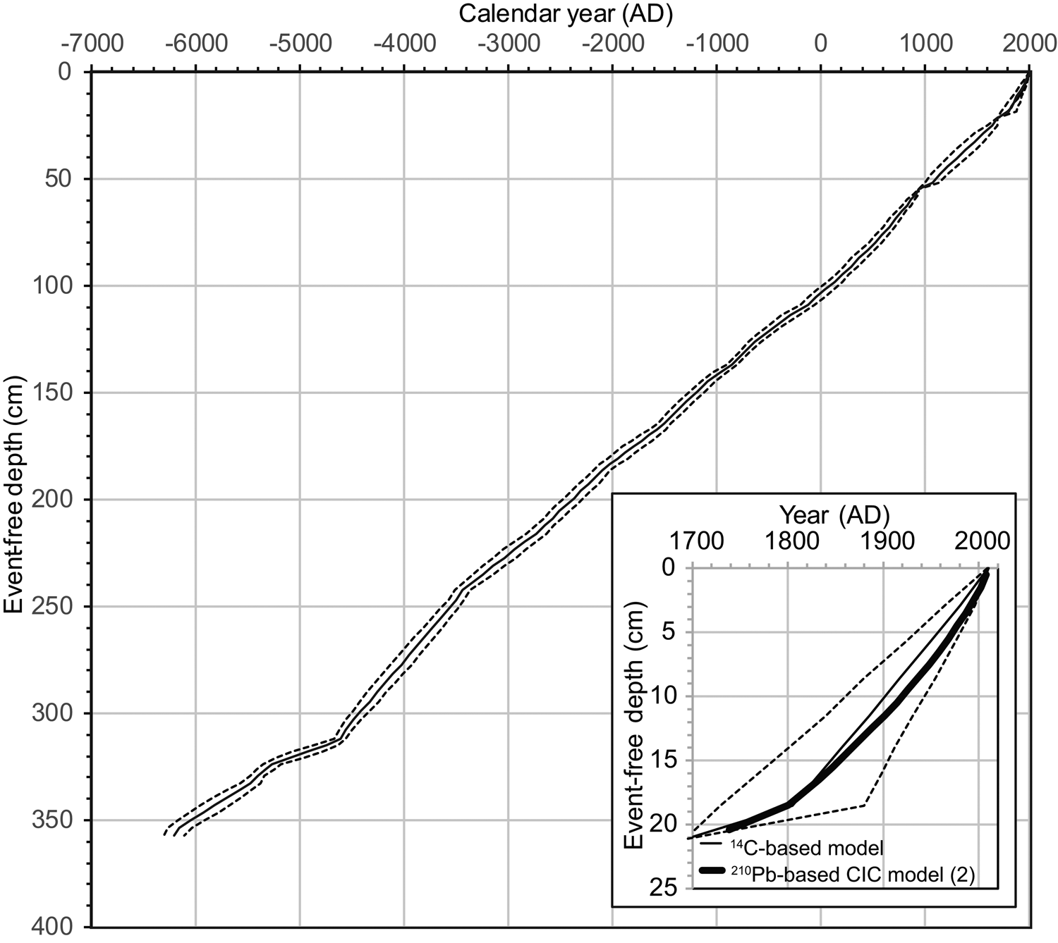
Figure 4. Overall age-depth model for the T3 composite core. The ‘event-free’ depth (efd) of the composite is the depth below the sediment water interface determined by correlating the surface multi-core to the piston core, followed by removal of units determined to be turbidite and tephra deposits. The model below 21.1 cm efd (Ko-c2) was generated using a Bayesian approach on 17 14C ages that were constrained by well-dated tephra ages (Ko-c2, B-Tm, and Ko-g). Above 18.5 cm efd for core T3 MC4-1, the model was generated using 210Pb-based CIC model (2) (Supplementary Figure 5). Between the points 18.5 cm efd/1800 AD and 21.1 cm efd/1694 AD, ages were determined by linear interpolation. The region between the dashed lines denotes the 95% probability ranges of the calibrated age at each event-free composite-core depth. The lower right-hand panel expands the upper portion, denoting the 210Pb-based CIC model 2 (0–21.2 cm efd) and the 14C-based Bayesian model.
Bio-opal and quartz
Mean bio-opal concentrations were low between 1100 BC and AD 400, and increased and varied on centennial timescales after AD 400 (Fig. 5a). The mean MAR values (Fig. 6) showed very similar temporal patterns to the concentrations (r = 0.84, P < 0.01, N = 90; Supplementary Table 3), whereas abnormally high values were observed after AD 1800 (Fig. 6a) in association with high sedimentation rates during this period. There was no trend in quartz concentrations before AD 1550, with decreased values thereafter (Fig. 5). Bio-opal concentrations showed a positive correlation with sedimentation rate (r = 0.45, P < 0.01, N = 87; Supplementary Table 3). In contrast, quartz concentrations (Fig. 5) show a negative correlation with sedimentation rate (r =−0.42, P < 0.01, N = 65; Supplementary Table 3). The bio-opal concentrations showed non-significant correlation with quartz content (r = 0.05, P > 0.01, N = 74; Supplementary Table 3).
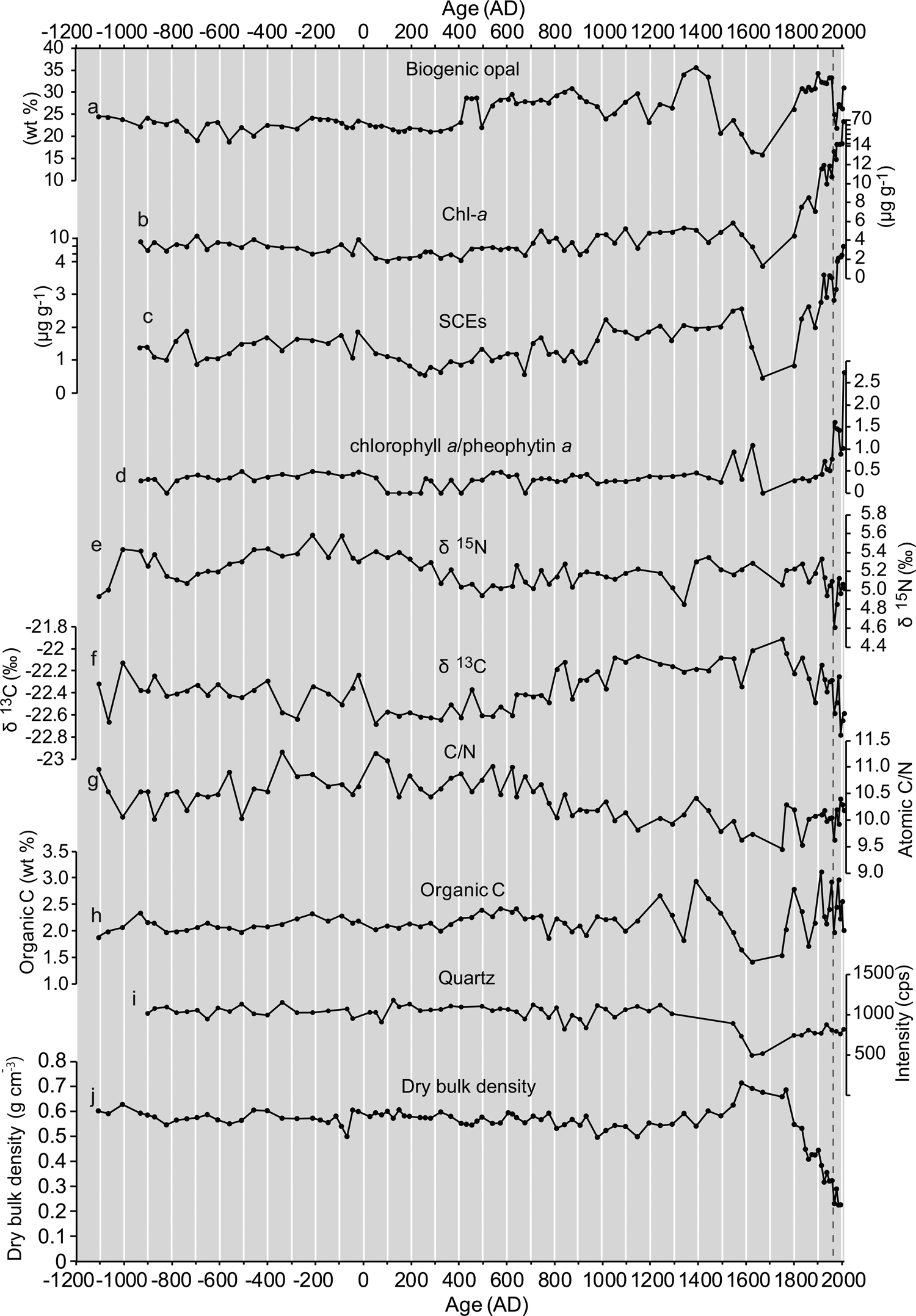
Figure 5. Temporal changes in concentrations of biogeochemical parameters in the T3 composite core. (a) Biogenic opal, (b) chlorophyll a and derivatives (Chl-a), (c) steryl chlorin esters (SCEs), (d) ratio of chlorophyll a/pheophytin a, (e) δ15N (sedimentary stable nitrogen isotope ratio), (f) δ13C (organic carbon isotope ratio), (g) C/N (molar ratio of organic carbon and nitrogen), (h) concentrations of total organic carbon (TOC), (i) quartz content, (j) dry bulk density. Vertical dashed line denotes 1960 AD, after which chlorophyll a/pheophytin a ratios and Chl-a and SCEs concentrations are high due to the presence of more undegraded labile chlorophyll a and SCEs in the surface sediments.
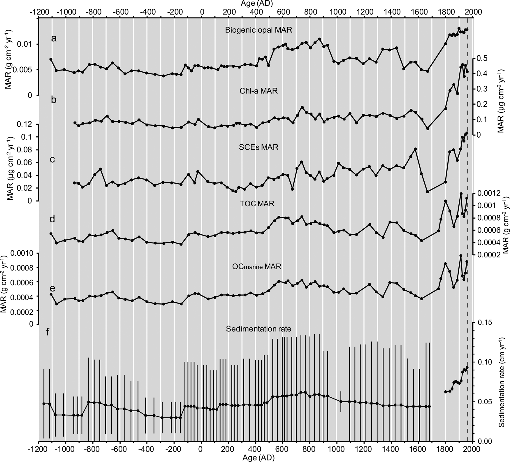
Figure 6. Temporal changes in mass accumulation rate (MAR) for biogeochemical parameters and sedimentation rate for the combined time series of T3 and T3 MC4-1 core before 1960 AD. (a) Biogenic opal, (b) chlorophyll a and derivatives (Chl-a), (c) steryl chlorin esters (SCEs), (d) total organic carbon (TOC), (e) δ13C-based marine-derived organic carbon (OCmarine), and (f) sedimentation rate; error bar for (f) denotes 95% confidence interval.
Pigments
Chl-a concentrations showed moderate values from 930 BC to 20 BC (mean: 3.5 μg g–1 dry sediment), low values from AD 50 to AD 700 (mean: 2.7 μg g–1), and an increasing trend from AD 700 to the twentieth century with centennial-scale variability (Fig. 5b). The SCEs (Fig. 5c) showed temporal patterns similar to those of Chl-a (r = 0.67, P < 0.01, N = 75). The mean MAR values of Chl-a and SCEs (Fig. 6b, c) showed very similar temporal variability to the concentrations (r = 0.995, P < 0.01, N = 76 for Chl-a; r = 0.980, P < 0.01, N = 76 for SCEs), whereas abnormally high values were observed after AD 1800. The MAR of Chl-a and SCEs showed a close correlation from 930 BC to AD 2008 (r = 0.98, P < 0.01, N = 76; Supplementary Table 3). Concentrations of Chl-a and SCEs showed a close positive correlation with sedimentation rate (r = 0.84, P < 0.01, N = 76; r = 0.85, P < 0.01, N = 76; Supplementary Table 3). In contrast, the concentrations of Chl-a and SCEs showed non-significant correlation with quartz content (r = -0.22, P = 0.06, N = 78; r =−0.29, P = 0.011, N = 78; Supplementary Table 3).
The weight ratio of chlorophyll a/pheophytin a showed no increasing trend before AD 1960, except for intervals of an abnormal peak (Fig. 5d), indicating nonsignificant effects of post-depositional degradation of pigments before AD 1960. After AD 1960 (0–6.5 cm depth in core), chlorophyll a/pheophytin a showed an increasing trend with abnormally high values. These high-value intervals indicate that there is more abundant labile chlorophyll a in the surface layer than in the other levels. The increase in Chl-a and SCEs after AD 1960, therefore, indicates a post-depositional degradation pattern. We excluded the surface Chl-a and SCEs data to observe long-term productivity changes and for PCA.
δ15N and δ13C, C/N, and TOC
Both δ15N and C/N showed a decreasing trend after AD 400, whereas δ13C showed an increasing trend after AD 400 and a decreasing trend after AD 1750 (Fig. 5). The organic carbon concentrations were relatively constant before AD 1100, and had large fluctuations after this time. The contributions of terrestrial organic carbon were estimated to be 15–30% or 13–36% of the TOC, based on δ13C or C/N, respectively. The MAR of δ13C- and C/N-based OCmarine showed an increasing trend with centennial-scale fluctuations after AD 400 (Fig. 6). There were similar temporal patterns between δ13C- and C/N-based OCmarine MARs (Supplementary Figure 8), which indicates the robustness of both estimations of the marine-derived carbon MAR.
Diatom assemblages
The results of diatom analysis showed that the most abundant diatoms were Chaetoceros spp. and its resting spores (53 ± 6%), followed by Odontella spp. (13 ± 5%), and Thalassiosira spp. and its resting spores (8 ± 2%) (Supplementary Figure 9). The diatom assemblages in the sediment core samples mostly were composed of Chaetoceros spp. and Thalassiosira spp. (61 ± 7%), of which their resting spores accounted for 86%.
The sum of percentages of sea-ice-associated species Bacterosira bathyomphala, Fragilariopsis oceanica, and Fragilariopsis cylindrus between AD 540 and AD 1950 showed centennial-scale variations during the past 1500 years, and were positively correlated with Chl-a concentration (r = 0.54, P < 0.01, N = 36), SCEs concentration (r = 0.60, P < 0.01, N = 36), Chl-a MAR (r = 0.52, P < 0.01, N = 36), and SCEs MAR (r = 0.64, P < 0.01, N = 36), and weakly correlated with bio-opal MAR (r = 0.35, P < 0.05, N = 36) (Supplementary Table 4).
The percentages of Fragilariopsis doliolus showed a negative correlation with the bio-opal concentration (r = −0.57, P < 0.01, N = 36) and MAR (r = −0.60, P < 0.01, N = 36), and a weakly negative correlation with Chl-a MAR (r = −0.41, P < 0.05, N = 36) but no correlation with Chl-a concentrations (Supplementary Table 4).
PCA of biogeochemical and mineral parameters
The results of the PCA conducted for the biogeochemical parameters revealed three main axes (PC1, PC2, PC3; see Fig. 7 for PC1 vs. PC2; Supplementary Figure 10 for PC1 vs. PC3), explaining 76% of the variations in all geochemical parameters (Supplementary Table 5). The highest loading of Chl-a was observed in PC1. SCEs and bio-opal were also highly loaded on PC1. The ratio of chlorophyll a/pheophytin a (chl a/pheo a) showed low loading on PC1. Dry bulk density is highly loaded on PC1, showing an inverse relation with bio-opal, Chl-a and SCEs. Organic carbon and nitrogen were perpendicular to δ13C, C/N, and chl a/pheo a. The inverse relation between dry bulk density and bio-opal, and moderate contributions of bio-opal concentrations to the total weight of dry sediment (10–30%) indicates that the abundance of diatom valves affects porosity in bulk sediment, which determines variations in the bulk density. Dry bulk density and bio-opal showed an oblique direction with δ13C and C/N (indices of mixing ratio of terrestrial and marine-derived organic matter) on PC1 vs. PC2 axes, indicating nonsignificant effects of dilution of terrestrial materials on dry bulk density and bio-opal. The highest loading of δ15N was found on PC3, although the other biogeochemical parameters were low loading on PC3 (Supplementary Figure 10).
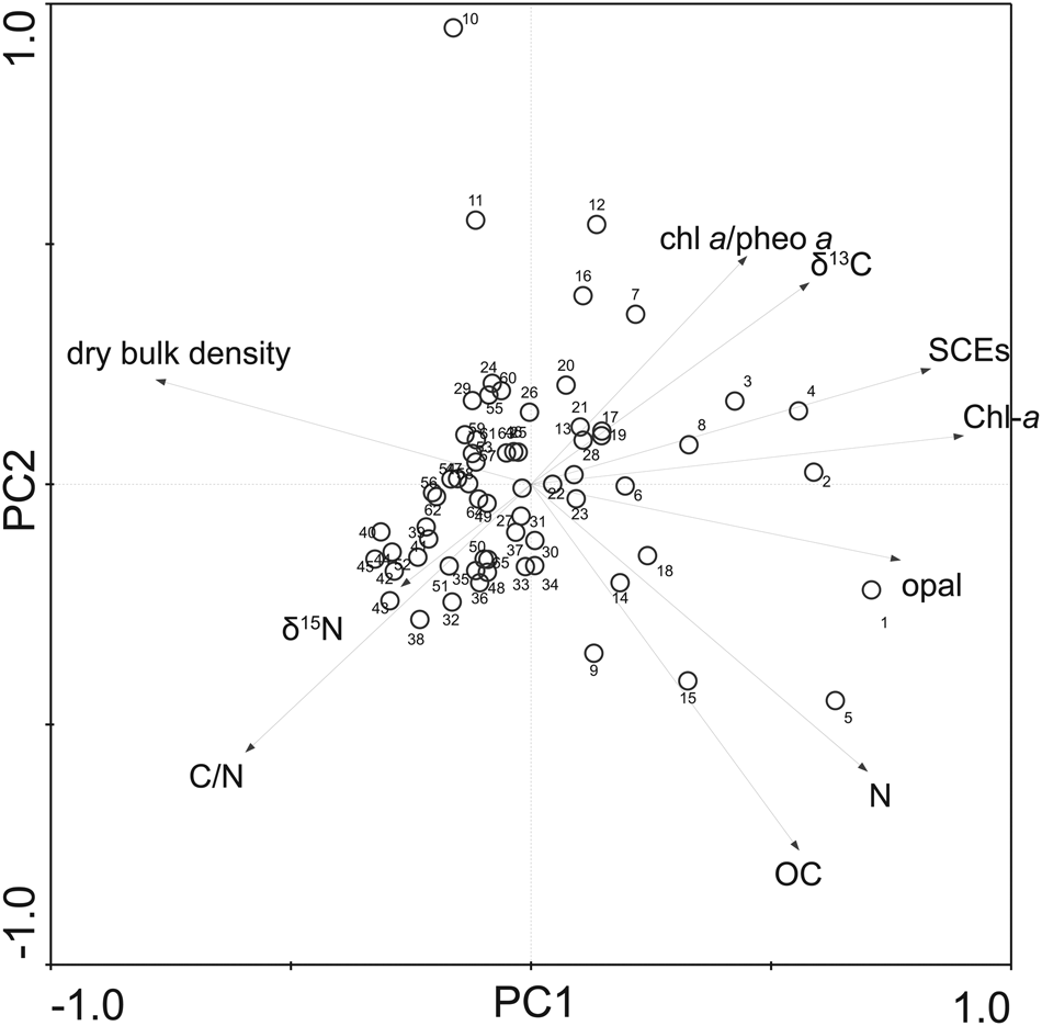
Figure 7. Principal component analysis (PCA) biplots of scores of biogeochemical indices in the principal component (PC) 1 versus PC2 axes. Chl-a: chlorophyll a plus derivatives concentrations, SCEs: steryl chlorin esters concentrations, chl a/pheo a: chlorophyll a/ pheophytin a ratio, OC: total organic carbon concentrations, N: total nitrogen concentrations, C/N: molar ratio of organic carbon and nitrogen, opal: biogenic opal (bio-opal) concentration, δ15N: sedimentary stable nitrogen isotope ratio, and δ13C: organic carbon isotope ratio. The first principal component (PC1) accounted for 44% of the variation, the second principal component (PC2) accounted for 18% of the variation, and the third principal component (PC3) accounted for 13% of the variation. These three components accounted for 76% of the variation. Numbers denote sample ID as described in Supplementary Table 5.
Results of PCA of mineral compositions, sedimentation rates, dry bulk density, Chl-a, SCEs, and bio-opal (Supplementary Table 6) showed that directions of mineral contents such as quartz, illite, chlorite, and other minerals, were perpendicular to Chl-a, SCEs, bio-opal, sedimentation rate, and dry bulk density on the PC1 and PC2 axes (Supplementary Figure 11). Dry bulk density had a negative correlation with Chl-a, SCEs, bio-opal, and sedimentation rate.
PCA of biogeochemical parameters and diatom assemblages
The results of the principal component analysis (PCA) conducted using biogeochemical parameters and diatom assemblage data were used to detect the leading factors of variability in lower trophic productivity indices (Supplementary Table 7). Chl-a, SCEs, resting spores of Chaetoceros furcellatus, and sea-ice-associated diatom species have a high positive contribution to PC1 (Supplementary Figure 12). Chl-a, SCEs, and sea-ice associated diatoms showed an inverse relation with Neodenticula seminae. In contrast, bio-opal, organic carbon, and δ13C exhibited moderate loadings on PC2. Organic carbon and bio-opal were positively correlated with the large diatom species Actinocyclus curvatulus, Coscinodiscus spp., and B. bathyomphala, and were negatively correlated with Chaetoceros resting spores and F. doliolus. Inverse directions between Chaetoceros resting spores and F. doliolus with bio-opal, organic carbon, and large diatoms indicated that the percentage of Chaetoceros resting spores decreased when productivity of large diatom was high. This mode of variability is less related to the PC1 mode, which is characterized by high contributions of Chl-a, SCEs, and sea-ice-associated diatoms.
DISCUSSION
Factors controlling biogeochemical concentrations
Concentrations of bio-opal, Chl-a, SCEs, and organic carbon may be influenced by availability of terrestrial or marine micro- and macronutrients through primary productivity in Hidaka Bay, and dilution effects of deposition rates of terrestrial clastic materials onto the bottom sediments. Primary productivity in Hidaka Bay is mainly driven by supply of macronutrients and iron from oceanographic sources. The influence of terrestrial macronutrients and dissolved iron on primary productivity are likely minor because the volume transport of the CO has a magnitude order of 106 m3/s (Sakamoto et al., Reference Sakamoto, Tsujino, Nishikawa, Nakano and Motoi2010), which is larger than a typical river discharge by five orders of magnitude (~10 m3/s for the Mu and Saru rivers), although the concentrations of nitrate plus nitrite are comparable between the rivers (10 μM) and CO during the pre-bloom period (15 μM) (Nishioka et al., Reference Nishioka, Ono, Saito, Sakaoka and Yoshimura2011). In general, dissolved iron from the river is expected to be removed from the water near the river mouth where river water encounters saline sea water for the first time (Boyle et al., Reference Boyle, Edmond and Sholkovitz1977). Therefore, only a very small amount of terrestrial dissolved iron from rivers directly reaches our observation site, and it has little effect on primary production because the site is located on the continental slope ~ 44 km from the nearest river mouth.
Dilution effects of deposition rates of terrestrial clastic materials on the concentrations of productivity indices are minor. Results from δ13C and C/N, indices of mixing ratio of terrestrial and marine-derived organic matter (Usui et al., Reference Usui, Nagao, Yamamoto, Suzuki, Kudo, Montani, Noda and Masao Minagawa2006; Kuwae et al., Reference Kuwae, Yamaguchi, Tsugeki, Miyasaka, Fukumori, Ikehara and Genkai-Kato2007), showed an oblique direction with dry bulk density and bio-opal with on PC1 vs. PC2 axes (Fig. 7). Furthermore, bio-opal, Chl-a, and SCEs showed no significant correlation with quartz content (Supplementary Table 3, Supplementary Figure 11), a proxy of inputs of terrestrial clastic materials. These results indicate that variations in dry bulk density, bio-opal, Chl-a, and SCEs are not substantially influenced by dilution of terrestrial materials. A close positive correlation between sedimentation rates with bio-opal, Chl-a, and SCEs (Supplementary Table 3, Supplementary Figure 11) indicates that deposition rates of marine production-derived materials are a main factor controlling sedimentation rates.
Chl-a and SCEs as proxies of spring biological productivity
The high positive loadings of Chl-a, SCEs, and bio-opal on PC1 (Fig. 7) suggest that the PC1 mode of variability is associated with variations in both primary and secondary production. The lack of an increasing trend of chl a/pheo a (Fig. 5), the different directions in the chl a/pheo a-vectors with Chl-a and SCEs on the PC1 and PC2 axes (Fig. 7), and the increasing trend of Chl-a and SCEs after AD 400 all indicate controls in Hidaka Bay by primary and secondary productivity as opposed to post-depositional pigment degradation. This is also supported by similar slopes of the linear regression line for δ13C and C/N and that of the two end-member trend (Supplementary Figure 13). If preferential degradation of organic nitrogen relative to organic carbon occurred through post-depositional processes, it would result in a steeper slope of a linear regression line of δ13C and C/N than that expected from the two end-member plots (i.e., terrestrial- and marine-derived organic matter; Usui et al., Reference Usui, Nagao, Yamamoto, Suzuki, Kudo, Montani, Noda and Masao Minagawa2006; Supplementary Figure 13). The similar slopes of both lines suggest that the preferential degradation of the nitrogen, contained in the molecular structure of chlorophyll a and its derivatives, and SCEs, is minor.
The results of the PCA analysis combining biogeochemical parameters with diatom assemblages showed different PC modes among bio-opal, organic carbon, and δ13C (PC2) with Chl-a and SCEs (PC1) (Supplementary Figure 12), indicating the presence of different mechanisms underlying the two PC modes. The high positive correlation between Chl-a and SCEs with sea-ice-associated diatoms indicates that the deposition of Chl-a and SCEs is associated with temporal variability in productivity during spring blooms in Hidaka Bay. Because C. furcellatus is the only diatom species observed as abundant resting spores in the CO during massive spring blooms (Kuroda et al., Reference Kuroda, Toya, Watanabe, Nishioka, Hasegawa, Taniuchi and Kuwata2019), the positive correlation of the resting spores with Chl-a and SCEs supports the inference of Chl-a and SCEs as a proxy of massive spring bloom productivity. In contrast, the positive correlation between bio-opal and organic carbon with the large diatom species Coscinodiscus spp., A. curvatulus, and B. bathyomphala indicates that the PC2 mode of variability is related to productivity of these large diatom species.
SCEs as a zooplankton biomass proxy
According to previous research, SCEs are formed by zooplankton grazing on phytoplankton (Harradine et al., Reference Harradine, Harris, Head, Harris and Maxwell1996; Talbot et al., Reference Talbot, Head, Harris and Maxwell1999a, Reference Talbot, Head, Harris and Maxwellb; Soma et al., Reference Soma, Itoh, Tani and Soma2005) and egested in fecal pellets (Harradine et al., Reference Harradine, Harris, Head, Harris and Maxwell1996; King and Wakeham, Reference King and Wakeham1996). Therefore, they can be used as a biomarker of grazing rates by zooplankton in a marine water column (Louda et al., Reference Louda, Loitz, Rudnick and Baker2000; Villanueva and Hastings, Reference Villanueva and Hastings2000; Soma et al., Reference Soma, Tanaka, Soma and Kawai2001; Squier et al., Reference Squier, Hodgson and Keely2002; Tani et al., Reference Tani, Kurihara, Nara, Itoh, Soma, Soma, Tanaka, Yoneda, Hirota and Shibata2002; Nara et al., Reference Nara, Tani, Soma, Soma, Naraoka, Watanabe, Horiuchi, Kawai, Oda and Nakamura2005). Because the grazing rates on phytoplankton most likely influence fecal pellet production and deposition in proportion to zooplankton biomass, the concentrations and MARs of SCEs represent zooplankton biomass. In particular, they might be inferred to reflect biomass during April–June, given that this interval corresponded to the time of highest biomass during two years of field observations near our core site E16 (Fig. 1; Shinada et al., Reference Shinada, Ban and Ikeda2008). Thus, the close correlation between the MARs of SCEs and Chl-a over the last two millennia indicates that long-term variations in zooplankton productivity from spring to early summer were controlled by spring phytoplankton productivity in this area.
Primary productivity indices in Hidaka Bay reflecting responses to centennial dynamics of CO
We hypothesize that the centennial variability in primary and secondary productivity observed in our pigment-derived records reflects response to changes in the frequency of CO intrusion into Hidaka Bay. There are several lines of indirect evidence to support this hypothesis (Table 1). First, the diatoms in the sediment samples were mostly neritic species: Chaetoceros genera and Thalassiosira genera. Observational studies have demonstrated that CO intrusions cause massive spring diatom blooms in the Oyashio areas (Kono and Sato, Reference Kono and Sato2010; Kuroda et al., Reference Kuroda, Toya, Watanabe, Nishioka, Hasegawa, Taniuchi and Kuwata2019) and in Funka Bay, which is the terminal position of westward intrusion of CO (Shinada et al., Reference Shinada, Shiga and Ban1999). Spring bloom producers primarily are composed of Chaetoceros and Thalassiosira genera (Kuroda et al., Reference Kuroda, Toya, Watanabe, Nishioka, Hasegawa, Taniuchi and Kuwata2019), most of which have higher iron requirements than oceanic species (Sunda and Huntsman, Reference Sunda and Huntsman1995). Kuroda et al. (Reference Kuroda, Toya, Watanabe, Nishioka, Hasegawa, Taniuchi and Kuwata2019) demonstrated that these genera are major components of massive spring blooms in response to CO water-mass intrusions. The major components of these genera in the sediments indicate that the temporal changes in bio-opal and Chl-a concentrations and their MARs are associated with variability in spring bloom productivity in response to CO intrusions, and associated macronutrient and iron fluxes.
Table 1. Four lines of evidence and the implication to support hypothesis of primary productivity in Hidaka Bay reflecting the responses to centennial dynamics of the iron-replete Coastal Oyashio. MAR: mass accumulation rate, Chl-a: concentrations of chlorophyll a and its derivatives, SCEs: steryl chlorin esters, HNLC: high-nutrient low-chlorophyll, OSIW: Okhotsk Sea Intermediate Water, CO: Coastal Oyashio.
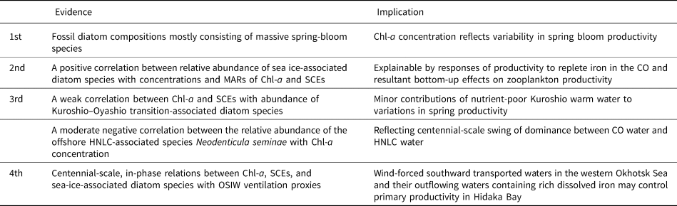
Second, the positive correlation between sea-ice-associated diatom species and concentrations and the MARs of Chl-a and SCEs, can be explained by responses of productivity to the transport of replete iron and Chaetoceros and Thalassiosira genera from the upstream of the CO area into Hidaka Bay and by bottom-up effects on zooplankton productivity.
The third line of indirect evidence is the minor influence of other water masses on the productivity of Hidaka Bay through nutrient availability for primary producers. Frequent intrusions of low-nutrient, warm, anticyclonic mesoscale eddies from the Kuroshio Extension might result in low primary productivity in the Oyashio and CO water. Ren et al. (Reference Ren, Gersonde, Esper and Sancetta2014) demonstrated that Fragilariopsis doliolus is abundant in the nutrient-poor Kuroshio Extension and the Kuroshio–Oyashio transitional water. Fragilariopsis doliolus is often observed in the Oyashio region during the spring bloom in association with the Kuroshio–Oyashio transitional water (Kuroda et al., Reference Kuroda, Toya, Watanabe, Nishioka, Hasegawa, Taniuchi and Kuwata2019). Therefore, the percentages of F. doliolus in the sediments are a possible index for temporal changes in the frequency of Kuroshio Extension-derived, nutrient-poor water intrusions in the study area. The weak correlation between Chl-a and SCEs with abundance of F. doliolus (Supplementary Figure 12; Supplementary Table 4) suggests minor contributions of Kuroshio Extension-derived water to variations in spring productivity at the study site. In contrast, the lateral transport of water mass from the western subarctic gyre, the so-called high-nutrient low-chlorophyll (HNLC) area, has a moderate negative influence on spring bloom because there is a moderate negative correlation between the relative abundance of the offshore HNLC-associated species Neodenticula seminae with Chl-a concentration (Supplementary Figure 12). This may reflect centennial-scale swings of dominance between CO water and HNLC water: times when CO intrusions are rare and HNLC water dominates result in the absence of massive spring blooms.
The fourth line of evidence is the association of centennial-scale, in-phase relations between Chl-a, SCEs, sea-ice-associated diatom species with OSIW ventilation inferred from both the sedimentary abundance of the radiolarian Cycladophora davisiana (Itaki and Ikehara, Reference Itaki and Ikehara2004) and epibenthic foraminifer δ13C (Lembke-Jene et al., Reference Lembke-Jene, Tiedemann, Nürnberg, Gong and Lohmann2018) that were reconstructed from the western Okhotsk Sea (sites GH01–1011 and LV28-4-4, respectively; Fig. 8). Outflow at the sea surface extending from the East Sakhalin Current and outflow in the intermediate layer tied to the OSIW are important pathways for the supply of iron into the western North Pacific (Nishioka et al., Reference Nishioka, Ono, Saito, Nakatsuka, Takeda, Yoshimura and Suzuki2007; Kuroda et al., Reference Kuroda, Toya, Watanabe, Nishioka, Hasegawa, Taniuchi and Kuwata2019). The East Sakhalin Current has two along-shore velocity maxima on the shelf and slope off the Sakhalin Island that can be barotropically controlled by alongshore wind stress through the dynamics of the arrested topographic waves (Csanady, Reference Csanady1978), and by basin-scale wind-stress curl through the dynamics of the Sverdrup balance (Simizu and Ohshima, Reference Simizu and Ohshima2006). Nakanowatari and Ohshima (Reference Nakanowatari and Ohshima2014) showed that alongshore transport on the Okhotsk shelf strengthened primarily when northeasterly winds prevailed off Sakhalin Island, which corresponded to negative values of the WP index (Horel and Wallace, Reference Horel and Wallace1981) and North Pacific Index (i.e., deepening of the Aleutian Low; Trenberth and Hurrell, Reference Trenberth and Hurrell1994). Likewise, if the basin-scale wind-stress curl changed the southward transport of the dense shelf water along the slope east of Sakhalin Island, which is the source water of OSIW, outflow of the OSIW might be affected by wind-driven circulation in the Okhotsk Sea. These outflowing waters with rich dissolved iron are transported to the downstream CO area near the sea surface or the Oyashio area through the intermediate layer, where the dissolved iron is eventually entrained into the euphotic zone by winter vertical convection and contributes to spring bloom formation (Nishioka et al., Reference Nishioka, Ono, Saito, Sakaoka and Yoshimura2011). These processes, in association with large-scale atmospheric forcing, can control localized primary productivity in Hidaka Bay, and are likely responsible for the coherent temporal patterns between Chl-a, SCEs, and sea-ice-associated diatom species with the OSIW ventilation indices.
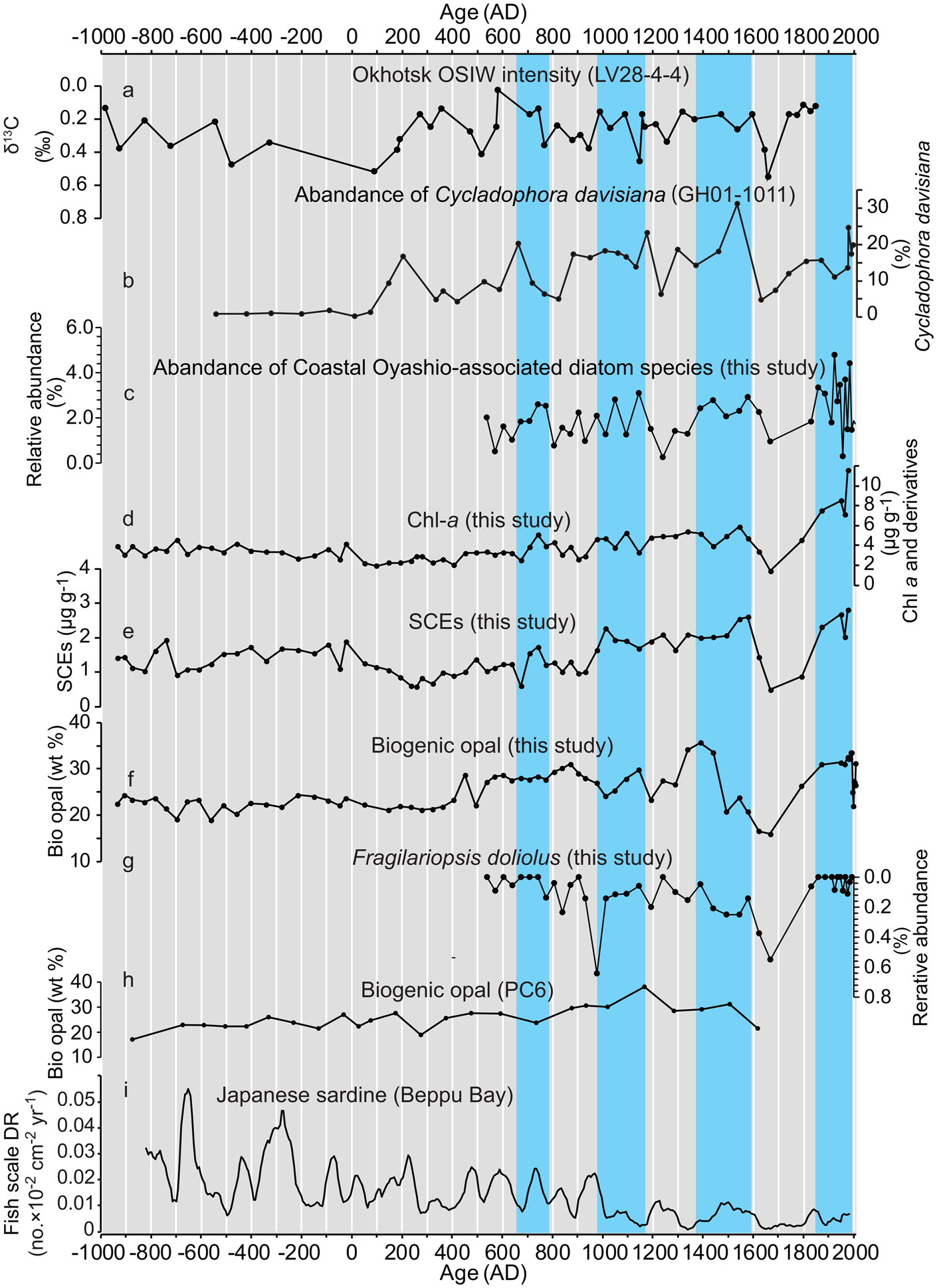
Figure 8. Temporal relationship between records of productivity indices in core sample T3 and other paleoceanographic proxies. (a) Okhotsk Sea Intermediate Water (OSIW) ventilation index from off East Sakhalin (LV28-4-4, 674 m water depth; Lembke-Jene et al., Reference Lembke-Jene, Tiedemann, Nürnberg, Gong and Lohmann2018), (b) relative abundance of Cycladophora davisiana (G01-1011, 1348 m water depth; Itaki and Ikehara, Reference Itaki and Ikehara2004), (c) relative abundance of Coastal Oyashio-associated diatom species (percentage sum of Bacterosira bathyomphala, Fragilariopsis oceanica, and Fragilariopsis cylindrus), (d) Chl-a (concentrations of chlorophyll a and its derivatives), (e) steryl chlorin esters (SCEs) concentrations, (f) biogenic opal concentrations (wt %: weight %), (g) relative abundance of Fragilariopsis doliolus, (h) biogenic opal concentrations (wt %: weight %) from PC6 site (Minoshima et al., Reference Minoshima, Kawahata and Ikehara2007), (i) deposition rate of Japanese sardine scales (Kuwae et al., Reference Kuwae, Yamamoto, Sagawa, Ikehara, Irino, Takemura, Takeoka and Sugimoto2017). Blue shade denotes interval of increased abundance of Coastal Oyashio-associated diatom species. (For interpretation of references to color in this figure legend, the reader is referred to the web version of this article.)
In summary, available circumstantial evidence, along with reasonable explanations for linkages between the proxies, support the hypothesis that long-term variability in spring primary and secondary productivity in Hidaka Bay mainly reflects the response to changes in the frequency of CO intrusion into the study area.
Forcing factors to account for the increasing trend in primary productivity in the CO region
Productivity proxies (Chl-a, SCEs, and bio-opal) showed an increasing trend in the records, especially after AD 400. This is consistent with an increasing trend during the Mid-to-Late Holocene reported as bio-opal concentrations in the CO (CH84-14, Crusius et al., 2004; Supplementary Figure 2) and downstream of the CO (PC6, Minoshima et al., Reference Minoshima, Kawahata and Ikehara2007). The Chl-a, SCEs, bio-opal, and marine-derived organic carbon MAR showed a twofold to fourfold increase from 3000 years ago to AD 1900 (Fig. 6). These increasing MARs might not have resulted from increased nutrient enrichment from the subsurface layer due to progressive intensified vertical convection in winter because there is no report of a decreasing trend in SST; rather, an increasing trend of winter SST reconstructed from foraminiferal δ18O in the adjacent site SK-2 has been reported (Sagawa et al., Reference Sagawa, Kuwae, Tsuruoka, Nakamura, Ikehara and Murayama2014). One possible mechanism is a progressively intensified CO with its resultant macronutrient and dissolved iron supply. This inference seemingly conflicts with the increasing trend in wintertime SST because decadal-scale SST changes tend to have an inverse relation with CO transport (Supplementary Figure 1). However, relative abundance of sea-ice-associated diatoms showed an increasing trend after AD 500 (Fig. 8, Supplementary Table 8) using the Mann-Kendall test (Kendall, Reference Kendall1938) for statistical significance, supporting an intensified CO. Increased CO transport is driven by enhanced winter northeasterly wind stress along the Sakhalin coast, which is associated with a negative WP mode. However, to test this mechanism in controlling productivity in the iron-replete CO and adjacent areas, a paleoclimate reconstruction for the WP index is required.
Implications of CO iron transport for sardine productivity
Japanese sardines spawn in the water off south Japan and transport and migrate into the Kuroshio Extension, Kuroshio–Oyashio transitional water, Oyashio, and Coastal Oyashio to grow (Fig. 1). The sedimentary record of sardine-scale deposition rate from Beppu Bay is most likely an excellent index of the regional sardine population in the Northwest Pacific because the bay is located near the main spawning grounds of Japanese sardine and there is general consistency between the historical catch records during the past 500 years in the sardine spawning areas off south Japan and that of sardine scale deposition rates (Kuwae et al., Reference Kuwae, Yamamoto, Sagawa, Ikehara, Irino, Takemura, Takeoka and Sugimoto2017). Currently, there is no information on long-term dynamics of prey abundance that would cause centennial variability in the sardine stock.
Although the lower trophic productivity showed an increasing trend in the downstream area of CO at sites T3 (Fig. 8f) and PC6 (Fig. 8h), it differs from Japanese sardine productivity, which shows a decreasing trend over the last 3000 years (Fig. 8). This indicates that iron supply rates associated with CO intrusions into the northwest Pacific do not necessarily contribute to the long-term variability of Japanese sardine productivity. Because Japanese sardine use other water masses, including the Kuroshio Extension, Kuroshio–Oyashio transition, and Oyashio, lower trophic level productivity needs to be elucidated in these water masses.
CONCLUSIONS
To elucidate the long-term dynamics of productivity in CO, which is a major pathway of iron supply to the surface layers in the northwest Pacific, temporal changes in primary and secondary productivity over the last 3000 years were reconstructed. Records of Chl-a (chlorophyll a and its derivatives), SCEs, bio-opal concentrations, and MARs showed an increasing trend and centennial-scale variability after ca. AD 400. The SCEs concentrations showed a high positive correlation with Chl-a concentrations, indicating that zooplankton productivity was controlled by bottom-up effects in CO. To test the hypothesis that centennial-scale, lower trophic productivity reflects a response to the intensity (frequency of intrusions) of CO with replete dissolved iron, we compared the temporal relation between the concentrations and MARs of Chl-a, SCEs, and bio-opal with the relative abundance of sea-ice-associated diatom species. There were close correlations between Chl-a and SCEs with sea-ice-associated diatoms, indicating that the lower trophic productivity was influenced by CO intensity, probably responding to iron supply from the western Okhotsk Sea.
Inconsistency between the long-term trends in Chl-a and SCEs with sardine abundance suggests that effects of CO iron transport on the sardine population through the bottom-up effect may be minor, if any. Other paleofish abundance reconstructions in the large marine ecosystems of the world's major fisheries have demonstrated long-term variability in the Gulf of Alaska (Finney et al., Reference Finney, Gregory-Eaves, Douglas and Smol2002), off North America (Baumgartner et al., Reference Baumgartner, Soutar and Ferreira-Bartrina1992; Tunnicliffe et al., Reference Tunnicliffe, O'Connell and McQuoid2001), off Peru and Chile (Valdés et al., Reference Valdés, Ortlieb, Gutierrez, Marinovic, Vargas and Sifeddine2008; Gutiérrez et al., Reference Gutiérrez, Sifeddine, Field, Ortlieb, Vargas, Chávez and Velazco2009; Salvatteci et al., Reference Salvatteci, Gutierrez, Field, Sifeddine, Ortlieb, Caquineau, Baumgartner, Ferreira and Bertrand2019), and South Africa (Struck et al., Reference Struck, Altenbach, Emeis, Alheit, Eichner and Schneider2002). To better understand long-term ecosystem variability and regulating processes, including food chains and their bottom-up or top-down control, and to validate the ecosystem–climate hypothesis (Finney et al., Reference Finney, Alheit, Emeis, Field, Gutiérrez and Struck2010), additional sedimentary records of lower trophic productivity are required for these systems. Our study highlights the utility of chlorophyll a and its derivatives and SCEs to reveal long-term variability in lower trophic level productivity.
Acknowledgments
We thank all of the crew of R/V Tansei-maru (KT-10-5) for the sampling and Dr. Koji Sugie of Japan Agency for Marine Earth Science and Technology and Dr. Kazuaki Tadokoro and Dr. Tsuyoshi Watanabe of Fisheries Resources Institute, Japan Fisheries Research and Education Agency for providing comments to improve our paper.
Supplementary material
The supplementary material for this article can be found at https://doi.org/10.1017/qua.2021.71
Financial support
This study was supported by the 2008–2012 Special Coordination Funds for Promoting Science and Technology from the MEXT and Grants-in-Aid for Scientific Research (22340155, 17H02959, 18H01292) from the JSPS. The cooperative research program (10A020, 09A025) of the Center for Advanced Marine Core Research, Kochi University supported this study.


 Open access