


INTRODUCTION
Although the importance of the tropics as a major driver of global climatic systems and hydrological cycles has been previously highlighted (e.g., Chiang, Reference Chiang2009), current knowledge of how long-term environmental change has affected these regions and their hydrological responses to past environmental change is limited (Metcalfe and Nash, Reference Metcalfe and Nash2012). As a prime example, the tropical savanna region of northern Australia (that covers 23% of the continent) (Fig. 1), exhibits large temporal and spatial gaps in research coverage. The longest (and continuous) terrestrial record from within the Australian savanna currently extends to the last glacial maximum (Rowe et al., Reference Rowe, Wurster, Zwart, Brand, Hutley, Levchenko and Bird2021). The availability of proxies is limited by seasonal conditions in the northern Australian tropics, restricting most records to the coastal zone or the Atherton Tablelands (Field et al., Reference Field, Tyler, Gadd, Moss, McGowan and Marx2018). There is also a disparity in the spatial distribution of records. Most derive from coastal zones (Prebble et al., Reference Prebble, Sim, Finn and Fink2005; Proske et al., Reference Proske, Heslop and Haberle2014; Proske, Reference Proske2016). The few records from the northeast of Australia (Cape York Peninsula) begin during the middle Holocene and are limited to one or two proxies per study (Luly et al., Reference Luly, Grindrod and Penny2006; Proske et al., Reference Proske, Stevenson, Seddon and Taffs2017) (Fig. 2, Table 1). This situation differs from the wet tropics of eastern Australia, and particularly the Atherton Tablelands, where numerous studies have revealed the climatic and environmental conditions that prevailed during the last 50 ka (Haberle, Reference Haberle2005; Turney et al., Reference Turney, Kershaw, James, Branch, Cowley, Fifield, Jacobsen and Moss2006; Muller et al., Reference Muller, Kylander, Wüst, Weiss, Martinez-Cortizas, LeGrande, Jennerjahn, Behling, Anderson and Jacobson2008; Kershaw and van der Kaars, Reference Kershaw, van der Kaars, Metcalfe and Nash2012; Burrows et al., Reference Burrows, Heijnis, Gadd and Haberle2016).
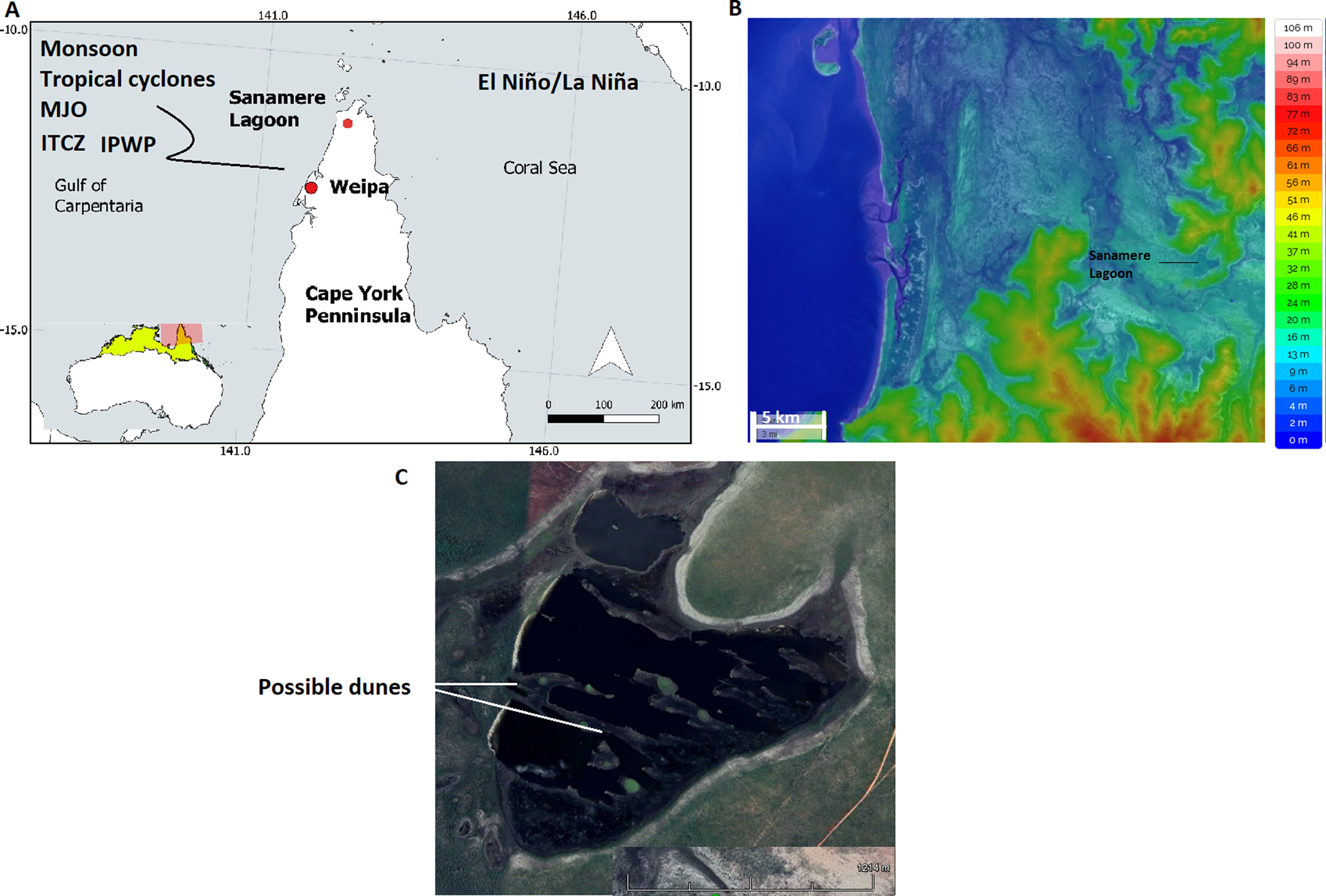
Figure 1. (A) Location of Sanamere Lagoon in Cape York Peninsula and main drivers of climate in the region; yellow area = tropical savannas in Australia, green area = wet tropics; ITCZ = Intertropical Convergence Zone; IPWP = Indo-Pacific Warm Pool; MJO = Madden-Julian Oscillation. (B) Topography of surrounding area (map modified from topographic-map.com). (C) Location of possible dunes in the site.

Figure 2. Locations of sites mentioned in the text, with a focus on Cape York and surrounding areas (refer to Table 1).
Table 1. Sites with paleoenvironmental evidence in the tropics of Australia.

Biogeochemical records derived from lake sediments have proven useful across a range of geographical areas to identify changes in climate, precipitation, and anthropogenic activities (Meyers and Lallier-Vergès, Reference Meyers and Lallier-Vergès1999; Leng and Marshall, Reference Leng and Marshall2004). It is the ability of lake sediments to integrate catchment-wide fluctuations in terrestrial and aquatic processes over long timescales that makes them so useful (Cohen, Reference Cohen2003). Especially relevant are records with robust dating and quality preservation of multiple proxies. The combination of several proxies provides the opportunity to validate and interrogate current hypotheses regarding the trajectory of past environmental change (Birks and Birks, Reference Birks and Birks2006). The limitations of any method may be contained and balanced through the strengths of partner proxies. The study of these biogeochemical responses, preserved in a range of proxy records, provides a better understanding of past climate drivers in the study region, including the Indonesian-Australian summer monsoon (IASM), the position of the Intertropical Convergence Zone (ITCZ), and the dynamics of the Indo-Pacific Warm Pool (IPWP) and the Madden-Julian Ocillation (MJO), all of which drive northern Australian climate and hydrology (Risbey et al., Reference Risbey, Pook, McIntosh, Wheeler and Hendon2009; Krause et al., Reference Krause, Gagan, Dunbar, Hantoro, Hellstrom, Cheng, Edwards, Suwargadi, Nerilie and Rifai2019).
Given the extension of the northern Australian tropics, studies report different evidence regarding the timing and intensity of monsoon peak activity over different time scales and monsoon reactivation during the deglacial. For example, some records show wet conditions over tropical Australia during the last glacial maximum (LGM) (records from South Indonesia, Ayliffe et al., Reference Ayliffe, Gagan, Zhao, Drysdale, Hellstrom, Hantoro and Griffiths2013), while other proxies indicate drier conditions (northern Western Australia, Di Nezio and Tierney, Reference Di Nezio and Tierney2013; Denniston et al., Reference Denniston, Asmerom, Polyak, Wanamaker, Ummenhofer, Humphreys, Cugley, Woods and Lucker2017). There are also discrepancies around the impact of climate change during Heinrich Stadials and the relative intensity of the monsoon system. Questions over the status of the monsoon are especially acute during the middle into late Holocene, where climatic processes overall are known to show a high degree of variability (Lewis et al., Reference Lewis, Gagan, Ayliffe, Zhao, Hantoro, Treble and Hellstrom2011). Exploring these variabilities within a sub-region of the Australian savanna environment in Cape York Peninsula is a valuable contribution to the reconstruction of the local patterns of environmental change.
This paper presents a paleoclimatic and hydrological record from Sanamere Lagoon, located at the northernmost point of Cape York Peninsula. Sanamere is the first continuous terrestrial record covering the last ca. 33,000 yrs BP of environmental change from the lowland tropics of northeastern Australia. This record consists of lake sediment-derived geochemical (micro X-ray fluorescence [μXRF] scanning, carbon and nitrogen content and their stable isotopes), physical (grain size), and biological (diatoms) proxy datsets. We develop a record of hydroclimatic changes for this under-studied region of northeast Australia and examine this record in the context of other records developed for the region.
SITE DESCRIPTION
Cape York Peninsula (here-in referred to as ‘the Peninsula’) stretches between 10°S and 16°S and is one of the major monsoon-influenced regions of Northern Australia, along with the Kimberley in Western Australia and the Northern Territory's ‘Top End.’ Most of the Peninsula has a strongly seasonal tropical climate (also referred to as monsoonal) (Peel et al., Reference Peel, Finlayson and McMahon2007), with just a small area of wetter climate (humid tropical) on the eastern coast (Fig. 1). Perennial lakes are scarce across the Peninsula, given high evapotranspiration rates and the limited rainfall over much of the year. As a consequence, sites permitting the study of long-term environmental change are limited and the location of any suitable lake sites particularly valuable.
Sanamere Lagoon (11.1230°S, 142.3594°E; 15 m above sea level [asl]) is located within the boundaries of the Apudthama Land Trust. The lagoon is 1 km north of the W-E flowing perennial Jardine River (Fig. 1), is ~2.5 km2 in area, with an approximate catchment area of 9 km2 overflowing through a low saddle to the west at ~17 m asl. The majority (88%) of the annual 1753 mm rainfall occurs between December and April, with a mean annual temperature of 27°C (Commonwealth of Australia, 2020). Although most lakes dry out in this region during the dry season, the deeper parts of Sanamere Lagoon have been permanently covered by standing water for the last 35 years (Mueller et al., Reference Mueller, Lewis, Roberts, Ring, Melrose, Sixsmith and Lymburner2016). This is despite periods of significantly below-average regional rainfall in this period (BOM, 2018). Maximum water depth during the dry season in 2017 was 1.2 m. At this level, several relict dune features are exposed, dating from the time of lagoon impoundment. During the wet season, these features are largely submerged and the lake flows into the Jardine River. The lagoon is immediately bordered by open sedges and Pandanus species, and the catchment is then occupied by heath. Beyond/surrounding the catchment is Eucalyptus-dominated woodlands (Neldner et al., Reference Neldner and Clarkson1995). The lake was probably formed as a result of the collapse of laterite karst to form a sinkhole-like depression below the local water table (Grimes and Spate, Reference Grimes and Spate2008).
METHODS
Sample collection
The sediment core was recovered from the approximate Lagoon center in July 2017. Cores were taken from the deepest portion of the lake in a single drive from a raft-mounted hydraulic coring rig. In total, 172.2 cm of sediment was collected, immediately cut into four sections, and frozen on site to enable transportation without disturbance. On return to the laboratory, the frozen cores were split lengthways, and one portion scanned at the Australian Nuclear Science and Technology Organisation (ANSTO) using the ITRAX μXRF core scanner. The remaining portion was sub-sampled for further analyses.
Stratigraphy and chronology
Core stratigraphy was defined by physical features (darkness, stratification, and texture), color, structure, visible components (organic fragments, charcoal), sedimentation rate, grain size, and carbon content. Variations in grain size can indicate changing transport energy, lake level, and the amount and energy of runoff into a sedimentary basin. The presence of larger grains in the sediment record indicates either increased precipitation (especially in closed-basin lake catchments) (Chen et al., Reference Chen, Wan, Zhang, Zhang and Huang2004; Conroy et al., Reference Conroy, Overpeck, Cole, Shanahan and Steinitz-Kannan2008) or lower lake stands that lead to shorelines prograding toward the lake center (Xiao et al., Reference Xiao, Chang, Wen, Zhai, Itoh and Lomtatidze2009). Thus, grain size can be used as an indicator for a change in water influx, although the direction of change cannot be inferred from grain size alone. Forty-one sediment samples (1, 5, 7, 10, 12, 23, 25, 28, 30, 32, 36, 38, 42, 44, 47, 52, 55, 58, 60, 63, 65, 67, 68, 69, 73, 75, 77, 79, 81, 83, 85, 87, 90, 93, 99, 105, 136, 141, 151, 162, 172 cm) were dispersed with sodium hexametaphosphate, sieved so particles <1000 μm could be retained, subsequently pretreated with 30% hydrogen peroxide (H2O2) to remove organics and finally with NaOH to dissolve biogenic silica particles. After this pretreatment, all samples were analyzed using a Malvern Mastersizer 2000 laser diffraction spectrophotometer. The median grain size and the percentages of clay (<2 μm), silt (≥2 μm, <63 μm), sand (≥63 μm), and coarse sand (≥275 μm, <1000 μm) were obtained for each depth.
Details of the dating procedure can be found in Rivera-Araya et al. (Reference Rivera-Araya, Rowe, Levchenko, Ulm and Bird2022) and Figure 3. In summary, six different organic fractions (bulk organics, pollen concentrate, cellulose, stable polycyclic aromatic carbon (SPAC), macrocharcoal >250 um, and microcharcoal >63 um) were compared at six different depths along the core. Acid-base-acid (ABA), modified ABA (30% hydrogen peroxide + ABA), 2chlorOx (a novel cellulose pre-treatment method), and hydrogen pyrolysis (hypy) were used to pre-treat the organic fractions. All samples were calibrated to calendar years using the Oxcal Program and the IntCal13 calibration curve (Reimer et al., Reference Reimer, Bard, Bayliss, Beck, Blackwell, Ramsey and Buck2013) with 0 calibrated years before present representing 1950 AD. IntCal13 was used rather than SHCal13 due to the influence of Northern Hemisphere air masses on the Tropical North of Australia, when the Inter Tropical Convergence Zone moves southwards during the Australian-Indonesian summer monsoons (Hogg et al., Reference Hogg, Hua, Blackwell, Niu, Buck, Guilderson and Heaton2013). The rbacon R package (Blaauw and Christen, Reference Blaauw and Christen2019) was used to develop the age models for the core.

Figure 3. Age-depth model for the Sanamere Lagoon (95% confidence error bars) constructed using Bayesian age modeling with the rbacon package in R (Rivera Araya et al., Reference Rivera-Araya, Rowe, Levchenko, Ulm and Bird2022). Ages were interpolated for each sampled depth and sedimentation rates were calculated over 1 cm intervals using the number of years covered by that interval as indicated by the age-depth model.
Rivera-Araya et al. (Reference Rivera-Araya, Rowe, Levchenko, Ulm and Bird2022) found that the magnitude and consistency of offsets between fractions and the physical and chemical properties of the tested organic fractions indicate that SPAC is the most reliable fraction to date in Sanamere Lagoon and that hypy successfully removes contamination sourced from exogenous carbon. The oldest date is 31,300 calibrated years before present (cal yr BP) and the youngest is 2500 cal yr BP, spanning ca. 29,000 years.
The source of organic matter in the lagoon sediments was investigated using bulk sedimentary nitrogen and organic carbon isotope values, as well as the carbon-to-nitrogen (C:N) ratios. The biochemical and organic matter composition of the biota in a lake depends on the amount and types of organic matter deposited at different times in the history of the site. C:N ratios often have been used to distinguish the origins of sedimentary organic matter, with algae having ratios between 5–8 and vascular plants >20, while ratios of ~10–20 mark the transition from primarily aquatic (<10) to primarily terrestrial (>20) sources (Meyers and Ishiwatari, Reference Meyers and Ishiwatari1993, Reference Meyers, Ishiwatari, Lerman, Imboden and Gat1995). Carbon isotopes of terrestrial organic matter can be used to track variations derived from the delivery of organic matter from C3 and C4 plants, moisture, and partial pressure of CO2 (Farquhar et al., Reference Farquhar, O'Leary and Berry1982). The carbon isotope composition of algal organic matter also reflects the availability of dissolved CO2. Although nitrogen isotopes have been associated with several indicators, including organic matter sources, past mixing regimes, and the history of nutrient loading (Talbot, Reference Talbot, Last and Smol2002; Brodie et al., Reference Brodie, Casford, Lloyd, Leng, Heaton, Kendrick and Zong2011), a possible inverse relationship between nitrogen isotope values and rainfall has also been suggested for the savannas in Northern Australia (Bird et al., Reference Bird, Brand, Diefendorf, Haig, Hutley, Levchenko and Ridd2019).
In total, 134 samples were analyzed for carbon and nitrogen abundance and isotope composition (δ13C and δ15N values). A representative aliquot of each sample was homogenized using a mortar and pestle. Total organic carbon and nitrogen abundance and isotope composition (aliquots 1–10 mg) were determined using a Costech elemental analyzer fitted with a zero-blank auto-sampler coupled via a ConFloIV to a ThermoFinnigan DeltaV PLUS using continuous-flow isotope ratio mass spectrometry (EA-CF-IRMS) at James Cook University's Cairns Advanced Analytical Centre. Stable isotope results are reported as per mil (‰) deviations from the VPDB and AIR reference standard scale for δ13C and δ15N values, respectively. Uncertainty on internal standards (‘Low Organic Carbon’ δ13C, −26.54‰; δ15N, 7.46‰; ‘Taipan’ δ13C, −11.65‰; δ15N, 11.64‰; and ‘Chitin’ δ13C, −19.16‰; δ15N, 2.20‰) was better than ±0.1‰. Repeated measurements on samples showed that C and N concentrations were generally reproducible to ±1% (1σ).
Elemental abundance
ITRAX analysis provides information about the variation in elemental abundance downcore. The abundances of elements such as iron (Fe), titanium (Ti), and aluminum (Al) in lake sediments typically indicate times of low lake level stands or greater clastic material transport under conditions of higher precipitation and consequent runoff (Douglas et al., Reference Douglas, Brenner and Curtis2016). XRF elemental profiles were completed in four sections (0–50, 50–100, 100–150, 150–172 cm), using the second-generation ITRAX core scanner located at the Australian Nuclear Science and Technology Organisation (ANSTO). Although the scanner produced data for a total of 25 elements (Al, Si, S, Cl, Ar, K, Ca, Ti, V, Cr, Mn, Fe, Ni, Cu, Zn, Br, Rb, Sr, Y, Zr, Pd, Ba, La, Ce, Pb), only those with above-background measurements and explanatory power for the environmental context in Sanamere Lagoon were selected for comparative analyses (Al, Si, Ti, Fe). In order to determine if a measurement was valid, the sample surface, argon, and total counts were analyzed for anomalous and/or inconsistent readings. The four selected elements were then normalized by calculating the proportion of counts of each element per total counts at each depth (Rothwell and Rack, Reference Rothwell and Rack2006), and a 10-point running mean calculated for the normalized concentrations, which gave an effective sample interval of 1 cm. To account for variations in moisture content, surface roughness, and grain size, ITRAX data were normalized against the total counts per second (Ohlendorf at al., Reference Ohlendorf, Wennrich, Enters, Croudace and Rothwell2015). Si:Ti ratios are interpreted as a measurement of biogenic silica (Davies et al., Reference Davies, Lamb and Roberts2015) and Si:Al ratios are used as proxies for grain size (Turner et al., Reference Turner, Jones, Brewer, Macklin, Rassner, Croudace and Rothwell2015). The ratio of incoherent (inc) to coherent (coh) dispersion depends on the average atomic number of the sediment material (Rothwell and Rack, Reference Rothwell and Rack2006), which generally correlates with organic carbon content (Burnett et al., Reference Burnett, Soreghan, Scholz and Brown2011) because the organic elements have average atomic weights smaller than aluminosilicates or quartz.
Stratigraphic units were delineated using hierarchical clustering and a broken stick model using the R packages vegan (Oksanen et al., Reference Oksanen, Blanchet, Friendly, Kindt, Legendre, McGlinn and Minchin2019) and rioja (Juggins, Reference Juggins2017), with Euclidean distance and constrained cluster analysis by the incremental sum of squares (CONISS) as the clustering method. The broken stick model separates the data into intervals and fits a separate line segment to each interval. This model is considered one of the best criteria that helps determine how many axes represent ‘important’ variation with respect to the original data table (Birks et al., Reference Birks, Lotter, Juggins and Smol2012).
Diatoms
Diatoms are widely used as indicators of paleoenvironmental conditions owing to their specific water quality preferences according to nutrient availability, acidity, light, thermal conditions, and dissolved oxygen concentrations (Stoermer and Smol, Reference Stoermer and Smol2001; Battarbee et al., Reference Battarbee, Jones, Flower, Cameron, Bennion, Carvalho, Juggins, Smol, Birks, Last, Bradley and Alverson2002). On Cape York Peninsula, diatom composition is correlated with total alkalinity, bicarbonate concentration, pH, electrical conductivity (EC), and latitude (Negus et al., Reference Negus, Barr, Tibby, McGregor, Marshall and Fluin2019).
The core was sampled every second centimeter between 1–43 cm and every three centimeters below 43 cm. Sample processing followed standard techniques, including sample deflocculation, oxidation of organic matter by addition of 30% hydrogen peroxide, isolation of diatom frustules by heavy liquid separation (s.g. = 2.15 g/cm3), and centrifugation for 15 minutes at 1500 rpm (Morley et al., Reference Morley, Leng, Mackay, Sloane, Rioual and Battarbee2004). The light fraction was then transferred by pipette to a clean tube. Samples were diluted to 4 mL and an aliquot transferred to a microscope slide for counting using a Nikon Eclipse TE300 microscope. The volume in the tube and the volume pipetted onto the slide were recorded, so the concentration of diatoms per sample could be calculated. Each sample was counted until at least 300 complete valves were identified or 10 transects were counted from each slide. Diatoms were identified using various taxonomic guides (Gell et al., Reference Gell, Sonneman, Reid, Illman and Sincock1999; Sonneman et al., Reference Sonneman, Sincock, Fluin, Reid, Newall, Tibby, Gell and Tyler1999). The relative abundance of each species was calculated as a proportion of the total, and species representing <2% of the relative abundance were removed to account for the influence of rare species. Raw diatom counts were converted to relative abundance before statistical analysis. The diatom assemblage was summarized and used to delineate zones using hierarchical clustering and a broken stick model, as described previously in the elemental abundance section.
RESULTS
Stratigraphy and chronology
Four initial stratigraphic zones were identified based on variations in the basic physical and chemical parameters along the core. The core description follows a sequence starting at the bottom of the core, with the last section referring to the top of the core. The first (lowest) layer (172–140 cm) is a dark brown color (5 YR 5/8), with carbon content <0.5%. Over the interval from 140–65 cm, mineral content gradually decreases and the color changes to light brown (7.5 YR 4/3). A series of three orange (7.5 YR 6/8) 1-cm thick bands are evident from 71–65 cm (Fig. 4). Beginning at 65 cm, the sediment color changes to reddish brown (5 YR 4/4). The upper 43 cm of the core consists of black (10YR 2/1), organic (5–40% carbon) sediments, including the presence of decomposed organic debris. Sedimentation rates change from 0.05 mm/year to 0.17 mm/year (Fig. 4) between 33–23.5 ka and range from 0.09–0.01 mm/year between 23.4–7.6 ka. Higher rates (0.09–0.15 mm/yr) are maintained towards the surface, until they drop abruptly at 4.9 ka, staying low until the end of the sequence (~ 0.01–0.09 mm/yr).

Figure 4. Sedimentation rates and grain size measured in the Sanamere sequence. Dashed lines indicate identified stratigraphic zones using clustering.
Particles <63 μm (i.e., silt and clay) dominate most of the Sanamere record (Fig. 4). Between 33–19 ka, percentages of sand are higher (up to 32% at 28.6 ka) compared to the rest of the sequence, where the percentage stayed <10%. Percentages of clay remain close to 20% between 33–30 ka and decrease to values <5% until 24 ka. These values then increase to 20% until the top of the sequence. The clay percentage broadly corresponds to the general trends seen in Ti counts. This correlation is most likely explained by the presence of anatase (metastable mineral form of titanium dioxide) derived from lateritic deep weathering, which forms a component of the fine fraction in the lateritic soils of the region (Eggleton et al., Reference Eggleton, Taylor, Le Gleuher, Foster, Tilley and Morgan2008). Percentages of coarse sand are <12% through the entire sequence, the one exception being an observation at 19 ka (26%) (Fig. 4).
The percentage of carbon ranges between 0.2–41% across the full core. Carbon abundance is consistent and low (0.3–1%) during the period 33–18.2 ka (Fig. 5). The period between 18.2–9.7 ka shows a sustained increase from 1% to 2.2%, from which point it gradually increases to 40% at 8.1 ka. Brief intervals of low abundance are evident until 4.3 ka, from which time values increase again. Nitrogen percentages range between 0.03–1.52% and follow a similar trend compared to carbon. The C:N ratio shows a gradual, but substantial, increase up the sequence, changing from a value of 4 at 32 ka to 13 at 10 ka. At 6.9 ka, the highest ratio is reached (44). From this point, the ratio declines to 11 at the end of the sequence (Fig. 5) δ13C values broadly decrease from the base of the record (−27‰) to 4 ka (~ −22‰) (with inter-interval fluctuations of usually ~ ± 0.5‰, but with individual short, larger excursions to individual values as high as −18‰ and as low as −29‰). From 4 ka to the present, values increase slightly to ~ −22‰ and remain constant. Nitrogen isotopes exhibit the same trends (noting variability between samples is generally larger, ± 1‰).

Figure 5. Total carbon, nitrogen, and isotopic abundance for the Sanamere sequence. Note that %C and %N are presented as log-transformed values. Dashed lines indicate identified stratigraphic zones using clustering.
Elemental abundance
High water content and low elemental counts prevented use of the XRF scanning results between 0–7 cm (present to ca. 4.2 ka). Cluster analysis (broken-stick) identified nine zones throughout the combined Sanamere profile, however four zones are used, consistent with the stratigraphic changes discussed above (Fig. 4). Fe has the highest relative counts in the spectra, followed by Ti (Fig. 6). Fe counts are stable and high from the bottom of the sequence (ca. 33 ka) until 10.8 ka from where they drop slightly (from 0.97 to 0.86). These counts fluctuate between 0.76–0.95 until they decrease abruptly to low values at 5.8 ka. After this, they increase again and fluctuate between 0.41 and 1 until they reach their lowest value at 4.8 ka, from which they peak again at 4.5 ka (Fig. 6). From the beginning of the sequence (bottom of the core) until 17.6 ka, Ti counts are high and exhibit only minor fluctuations (values between 0.68–0.80). At 17.6 ka, a decreasing trend is evident, with two major exceptions at 16.6 ka and 5.9 ka. Ti counts are also negatively correlated with Al counts.

Figure 6. Normalized elemental counts, elemental ratios, and ratio of incoherent (inc) to coherent (coh) dispersion. Dashed lines indicate identified stratigraphic zones using clustering.
Both Al and Si values stay low until 9 ka, thereafter, increasing to reach a peak ca. 7.5 ka, followed by an equally abrupt decrease ca. 5 ka. Si:Ti values show a peak at 8 ka, whereupon they decrease to reach previous values (Fig. 6). The inc/coh ratio increases at 11 ka and stays high until the top of the sequence. Higher values of Si:Al are evident from the bottom of the sequence until ca. 20 ka, and thereafter these values drop abruptly. Increased values are also evident at ca. 4.7 ka (Fig. 6).
Diatoms
Diatom abundance is low from the base of the sequence (850–1424 diatoms/g of sediment) to 21.2 ka, followed by a sustained increase in abundance to 10.9 ka. A peak in concentration is evident at 7 ka (~3 × 10⁵ diatoms/g), after which the concentration decreases abruptly. Values increase and return to early Holocene levels at the top of the core (Fig. 7). Although samples were extracted every 2 or 3 cm, samples between 120 cm and the bottom of the core did not yield sufficient diatoms to comply with the minimum required to derive statistically significant conclusions, except for samples at 132, 147, and 159 cm.

Figure 7. Diatom assemblage and concentration data. Dashed lines indicate identified stratigraphic zones using clustering.
Nineteen diatom species were identified. The assemblage is dominated by benthic diatoms with a preference for acidic environments throughout the record (although definitive conclusions about niche conservatism in diatom species is still premature; Soininen and Teittinen, Reference Soininen and Teittinen2019). Cluster analysis suggests the presence of three zones: ca. 33–18.2 ka, 18.2–7.3 ka, and 7.3 ka to present. Before 18.2 ka, the sequence is mostly dominated by Pinnularia viridiformis and Pinnularia stomatophora, with Stauroneis phoenicetron and Eunotia arcus as secondary species. At ca. 18.4 ka, the proportion of additional species (such as Brachysira brebissonii and Pinnularia sp.) increases, while P. viridiformis becomes less abundant. The diversity of species starts to increase at ca. 11 ka, and particularly after 9.8 ka, when Encyonema neomuelleri and Eunotia muscicola appear. At 7.3 ka, the abundance of B. brebissonii increases from values <6% to values >30%, while Pinnularia sp. decreases to values <10% for the rest of the sequence. From 4.3 ka, the relative abundance of B. brebissonii declined from 54% to values <17%, while Frustulia rhomboides increased, and species such as Eunotia diodon and Stenopterobia intermedia appeared for the first time.
DISCUSSION
Unit A (33–29.2 ka)
The age-depth model (Fig. 3) indicates that the sediments in Sanamere Lagoon started to accumulate ca. 33 ka. This likely occurred in a depression formed by collapse of the underlying laterite karst. This depression was then, and remains now, located below regional groundwater level, supporting initial water accumulation and the continued presence of a standing water body since formation. According to previous studies, accumulation of the initial sediments is likely to have occurred under dry climate conditions, before the major sea level drop at 30 ka, and even as water table reduced further into the LGM (Brooke et al., Reference Brooke, Nichol, Huang and Beaman2017) (Fig. 8). Between 33–30.1 ka, a possible wetter interval is suggested by high sedimentation rates (Fig. 4), associated with possible enhanced runoff of clastic sediment, with the highest percentage of clay in the sequence and an average particle size of 2.7 μm. Overall, climatic reconstructions in the region suggest drier and cooler conditions relative to the present, with the monsoon considered to be inactive or greatly weakened at this time (Reeves et al., Reference Reeves, Bostock, Ayliffe, Barrows, De Deckker, Devriendt and Dunbar2013). However, regional variations are starting to be demonstrated as more research is completed. Previous studies suggested a major latitudinal shift of the western Pacific ITCZ in southerly tropical regions (southern Papua New Guinea) during Heinrich Stadial 3 (ca. 30 ka), associated with intense rainfall (Lewis et al., Reference Lewis, Gagan, Ayliffe, Zhao, Hantoro, Treble and Hellstrom2011; Jacobel et al., Reference Jacobel, McManus, Anderson and Winckler2016; Bayon et al., Reference Bayon, De Deckker, Magee, Germain, Bermell, Tachikawa and Norman2017). The existence of wet periods during Marine Isotope Stages (MIS) 2 and 3 (30–18 ka) is similarly established for the wet tropics of Australia, including results from research at Broomfield swamp (Burrows et al., Reference Burrows, Heijnis, Gadd and Haberle2016) and Lynch Crater (Muller et al., Reference Muller, Kylander, Wüst, Weiss, Martinez-Cortizas, LeGrande, Jennerjahn, Behling, Anderson and Jacobson2008). Extreme floods have been identified during this same period (Nott et al., Reference Nott, Bryant and Price1999) further west in the Wangi Falls area in the Northern Territory (Nott and Price, Reference Nott and Price1994; Nott et al., Reference Nott, Price and Bryant1996), noting with caution that the Wangi Falls dates are potentially overestimated (May et al., Reference May, Preusser and Gliganic2015).

Figure 8. Sea level data extracted from Lambeck et al. (Reference Lambeck, Rouby, Purcell, Sun and Sambridge2014).
The ITRAX and grain size analyses indicate the presence of coarser quartz grains (higher Si:Al), and high concentration of Ti, both in accordance with the expected conditions after the lagoon formation under arid conditions during this period (Lambeck et al., Reference Lambeck, Rouby, Purcell, Sun and Sambridge2014; Brooke et al., Reference Brooke, Nichol, Huang and Beaman2017; Ishiwa et al., Reference Ishiwa, Yokoyama, Okuno, Obrochta, Uehara, Ikehara and Miyairi2019). Enriched values of δ15N suggest decreased rainfall, according to the significant inverse correlation between rainfall and δ15N found by Bird et al. (Reference Bird, Brand, Diefendorf, Haig, Hutley, Levchenko and Ridd2019) in northern Australia.
It is likely that during this time the site formed a shallow pond or swamp with low nutrient availability. These conditions likely supported the aquatic plants that dominated the lagoon during this period. The low concentration and autecology of the diatoms at the base of the column support this finding. For instance, P. viridiformis, a diatom that can be aerophilous, is the single dominant species during this period and is commonly found in neutral or acidic water. Aerophilous species commonly occur in subaerial environments, such as moist or temporarily dry places, to the point of surviving nearly exclusively outside water bodies (Johansen, Reference Johansen, Stoermer and Smol2010). The C:N ratios (<20) and δ13C values (< −25‰) suggest the input of aquatic plants or lacustrine algae, predominantly.
The end of this period is associated with an abrupt, further decrease in sea level (from −83 m to −126 m) that started ca. 30 ka (Lambeck, 2014). However, there are no apparent effects of this decrease in the Sanamere Lagoon sediments, despite this leading to a dramatic increase in the distance to the coast to both east and west of the site (Fig. 9 presents a summary of the paleoenvironmental history of the site).

Figure 9. Summary of environmental changes at Sanamere Lagoon.
Unit B (29.2–18.2 ka)
Site conditions appear to have remained relatively dry over the period between 29.2–18.2 ka (corresponding to much of MIS 2). δ15N values suggest decreased rainfall (increased aridity), a trend that is consolidated from the previous period. Rather than intermittent intervals of wetter conditions, a consistency developed in terms of a continual uninterrupted drying trend, but without the site actually drying out. Coarse grains, representing increased coarse sand (Fig. 4) and high values of Si:Al (Fig. 4), characterize this period, along with an increase in median grain size (from 2 μm to 11 μm). Diatoms continue to appear in low concentrations, although species in addition to P. viridiformis and E. arcus appear for the first time, including S. phoenicentron. These are all acidophilous species, recorded in habitats with running water (such as rivers and streams) (van Dam et al., Reference van Dam, Mertens and Sinkeldam1994). Diatoms from these habitats could indicate the presence of shallow and unstable environments (van Dam et al., Reference van Dam, Mertens and Sinkeldam1994). In the Sanamere Lagoon context, these habitats may be located between the raised elongated sand features that also likely formed during this period. Carbon and nitrogen concentrations continued to be low, indicating low production of biomass within the lagoon and the surrounding catchment.
Fluctuating water depths may have induced periodic deflation of exposed sediments on the Sanamere Lagoon shore, although the lake did not dry at the core location. During this time, dune formation and increased aeolian sedimentation took place in other locations in north and east Australia (Petherick et al., Reference Petherick, McGowan and Kamber2009; Lewis et al., Reference Lewis, Tibby, Arnold, Barr, Marshall, McGregor, Gadd and Yokoyama2020). These episodes of sand movement are coincident with periods of elevated IASM rainfall at Ball Gown Cave in Western Australia. These synchronous changes also link the responses of sites in western Kimberley and the Gulf of Carpentaria during the last glacial period (Denniston et al., Reference Denniston, Wyrwoll, Polyak, Brown, Asmerom, Wanamaker and LaPointe2013). Low sea levels during the LGM also influenced dune formation and emplacement on Cape York Peninsula and the Gulf of Carpentaria. Dune emplacements at Cape Arnhem (Lees et al., Reference Lees, Stanner, Price and Yanchou1995), Cape Flattery, and Shelburne Bay between 24–18 ka appear to represent a period of widespread dune activity associated with the LGM. Dune formation occurred at glacial low sea levels when wide areas of continental shelf became exposed to wind action (Lees et al., 1990; Lees, Reference Lees1992, Reference Lees2006).
Lagoons also record aeolian and dune activity. For example, in Native Companion Lagoon (NCL), in North Stradbroke Island (southeast Queensland), the significant local sand and dust content of the NCL record for this period indicate that the dunes surrounding NCL were active, most likely in response to a reduced cover of vegetation. The LGM is shown to be the period of maximum aeolian sand movement, as a result of decreased precipitation (Petherick et al., Reference Petherick, McGowan and Kamber2009). Loss of vegetation cover and subsequent destabilization of dunes would account for the increased deposition of local North Stradbroke Island sediments in Native Companion Lagoon at this time (McGowan et al., Reference McGowan, Petherick and Kamber2008; Petherick et al., Reference Petherick, McGowan and Kamber2009).
Increased coarse sand percentages in the Sanamere record (Fig. 4) agree with the postulated episodes of sand deposition (aeolian or fluvial origin) at 26 ka, 24 ka, and 21.5 ka in Lake Carpentaria to the west. These events were reported during a dry and cool period with large fluctuations of the Carpentaria lake level (Devriendt, Reference Devriendt2011). Furthermore, the sedimentary record at Lake Carpentaria indicates a temporary contraction of the lake to around the −63 m contour (23–19 ka), when the sea was at the lowest level (approximately −125 m) (Yokoyama et al., Reference Yokoyama, Purcell, Lambeck and Johnston2001; Brooke et al., Reference Brooke, Nichol, Huang and Beaman2017), and the Sahul shelf was fully exposed. The contraction of Lake Carpentaria likely increased aridity in the nearby Peninsula and reduced vegetation cover through a reduction in the water surface available for regional evaporation. The availability of sand and larger grains to be transported to the lagoon also increased, along with the formation of possible wind-blown sand dune features. Further evidence of increased wind activity comes from dust records across several sites in east and north Australia. These records have documented increased aeolian activity during this period (Shulmeister and Lees, Reference Shulmeister and Lees1992; Petherick et al., Reference Petherick, McGowan and Kamber2009; Lewis et al., Reference Lewis, Tibby, Arnold, Barr, Marshall, McGregor, Gadd and Yokoyama2020).
In the broader tropical Australasian region, most studies agree on evidence of drier, cooler conditions from late MIS 3 to the LGM (ca. 33 ka and 18 ka, respectively) (Denniston et al., Reference Denniston, Wyrwoll, Polyak, Brown, Asmerom, Wanamaker and LaPointe2013, Reference Denniston, Asmerom, Polyak, Wanamaker, Ummenhofer, Humphreys, Cugley, Woods and Lucker2017; Di Nezio and Tierney Reference Di Nezio and Tierney2013; Reeves et al., Reference Reeves, Bostock, Ayliffe, Barrows, De Deckker, Devriendt and Dunbar2013). Studies in the wet tropics of Australia also suggest drier and cooler conditions (33–18 ka) (Petherick et al., Reference Petherick, McGowan and Kamber2009). Lowered sea level and the exposure of the Sunda and Sahul shelves initiated changes in atmospheric circulation over the Indo-Pacific warm pool (IPWP) and these two factors contributed to large-scale regional drying during the LGM (Di Nezio et al., Reference Di Nezio, Timmermann, Tierney, Jin, Otto-Bliesner, Rosenbloom, Mapes, Neale, Ivanovic and Montenegro2016).
Studies in the region have proposed the LGM to be a particularly dry phase with an irregular monsoon (Hanebuth, Reference Hanebuth2000; Wyrwoll and Miller, Reference Wyrwoll and Miller2001; Hesse et al., Reference Hesse, Magee and van der Kaars2004; Reeves et al., Reference Reeves, Bostock, Ayliffe, Barrows, De Deckker, Devriendt and Dunbar2013). However, the Sanamere Lagoon record does not suggest this period to be particularly dry (according to the geochemical and biological evidence), nor that the exposure of the shelves locally had a significant effect on the hydroclimate of the site, and therefore by extension, at least the northernmost part of Cape York Peninsula. Recent modelling studies similarly suggest there was still an effective monsoon rainfall regime across the northern Australian region (Yan et al., Reference Yan, Wang, Liu, Zhu, Ning and Cao2018).
A mild LGM climatic effect for northern Cape York Peninsula may be explained by the position of the coastline, which was 900 km northwest of Sanamere Lagoon (Ishiwa et al., Reference Ishiwa, Yokoyama, Okuno, Obrochta, Uehara, Ikehara and Miyairi2019) during the LGM. Yan et al. (Reference Yan, Wang, Liu, Zhu, Ning and Cao2018) concluded that changes in land-sea distribution and east-west gradients in sea surface temperature resulted in a modest lowering of total rainfall (which would still feed the water table that was connected with the Lagoon), but an increase in rainfall seasonality across northern Australia. The change in coastline position probably decreased precipitation at any terrestrial site given the strong rainfall gradient into the interior.
This pattern of not extremely arid but drier climate is consistent with other studies from the area (Jiang et al., Reference Jiang, Tian, Lang, Kageyama and Ramstein2015; Denniston et al., Reference Denniston, Asmerom, Polyak, Wanamaker, Ummenhofer, Humphreys, Cugley, Woods and Lucker2017; Yan et al., Reference Yan, Wang, Liu, Zhu, Ning and Cao2018). Furthermore, the only terrestrial vegetation and fire records available from northern Australia (Girraween, Northern Territory) during this period also suggest dry, cool conditions during the LGM (Rowe et al., Reference Rowe, Wurster, Zwart, Brand, Hutley, Levchenko and Bird2021).
Unit C (18.2–9.7 ka)
The Ti counts show an increased magnitude in fluctuations starting at 20 ka, indicating episodic changes in the delivery of clastic sediments derived from around the lagoon as a result of changes in precipitation. Sedimentation reached its lowest rate, median grain size stayed the same (11 μm), and the diatom concentration remained the same as in the previous period. However, diatom species diversity did decrease, with only three species present: P. stomatophora, P. viridiformis, and B. brebissonii.
Between 17.6–12.8 ka, the lagoon recorded reactivation of the monsoon and increased moisture availability derived from the rise in post-glacial sea level, which also was recorded in wetter conditions and increased lake level for Lake Carpentaria (Devriendt, Reference Devriendt2011). The decrease in Ti counts at 14 ka and the decrease in grain size and Si:Al ratio during this time may be reflecting a substantial relative increase in the area of Lake Carpentaria, indicating wetter conditions and higher lake level, which may have limited the accumulation of clastic sediments in the center of the lake, which became increasingly remote from sources of sediment supply in the catchment. The increase in the C:N ratio at ca. 12 ka (Fig. 5) suggests an increase in higher plant organic input into the lagoon. These results are consistent with published studies indicating that the monsoon became active in northern Australia during this time period, (Hanebuth, Reference Hanebuth2000; Wyrwoll and Miller, Reference Wyrwoll and Miller2001; Hesse et al., Reference Hesse, Magee and van der Kaars2004; Reeves et al., Reference Reeves, Bostock, Ayliffe, Barrows, De Deckker, Devriendt and Dunbar2013; Field et al., Reference Field, Tyler, Gadd, Moss, McGowan and Marx2018; Rowe et al., Reference Rowe, Brand, Hutley, Wurster, Zwart, Levchenko and Bird2019).
Between 12.8–9.7 ka, trends in the biological and geochemical indicators suggest the existence of episodic wet events derived from an increase in rainfall associated with a stronger monsoon. During this period (in particular 12–9.7 ka), enriched δ15N values may be recording the input of nitrogen (inorganic and organic) from sources in the broader catchment, compared to previous periods described for Sanamere Lagoon. For example, at 10.8 ka, an increase in diatom concentration and the appearance of new diatom species (E. flexuosa, E. latum, E. neollimueri, E. pirla, Surirella spiralis) also indicate a change towards higher productivity conditions and further lake deepening, with some of these species (E. flexuosa, E. latum) preferring open water (Proske et al., Reference Proske, Heslop and Haberle2014). The C:N ratios (>20) and the δ13C values (< −25‰) record the input of terrestrial C3 plants. Increased δ15N values were probably driven by the further filling of the basin, with large amounts of nutrients released to the lagoon from the catchment as the lake filled (as in Talbot, Reference Talbot, Last and Smol2002). These changes in the lagoon are consistent with the increases in sea level (from ca. 12 ka) in Lake Carpentaria and the South Wellesley Archipelago (Sloss et al., Reference Sloss, Nothdurft, Hua, O'Connor, Moss, Rosendahl and Petherick2018), which brought a large source of moisture closer to the site. For instance, from 12 ka, oceanic waters transgressed the Arafura Sill, and by 10.7 ka, the Lake Carpentaria region had become marine (De Deckker et al., Reference De Deckker, Chivas, Shelley and Torgersen1988; McCulloch et al., Reference McCulloch, De Deckker and Chivas1989; Chivas et al., Reference Chivas, Garcia, van der Kaars, Couapel, Holt, Reeves and Wheeler2001). Sloss et al. (Reference Sloss, Nothdurft, Hua, O'Connor, Moss, Rosendahl and Petherick2018) found that sea level rose from −53 m (depth of the Arafura Sill; Harris et al., Reference Harris, Heap, Marshall and McCulloch2008; Reeves et al., Reference Reeves, Chivas, Garcia, Holt, Couapel, Jones, Cendón and Fink2008) at ca. 11.7 ka to ca. −25 m by 9.8 ka (Sloss et al., Reference Sloss, Nothdurft, Hua, O'Connor, Moss, Rosendahl and Petherick2018).
The Sanamere record is consistent with the increase in monsoon activity at ca. 12 ka suggested by several studies in the surrounding area (Wende et al., Reference Wende, Nanson and Price1997; Kuhnt et al., Reference Kuhnt, Holbourn, Xu, Opdyke, De Deckker, Röhl and Mudelsee2015; Field et al., Reference Field, Tyler, Gadd, Moss, McGowan and Marx2018). More locally, the rise in sea level facilitated increased moisture advection and tropical convection over Cape York. Warmer waters in parts of the IPWP region also contributed to amplify this effect (Griffiths et al., Reference Griffiths, Drysdale, Gagan, Zhao, Ayliffe, Hellstrom and Hantoro2009). However, the Sanamere record does not agree with the evidence of a strengthened IASM at ca. 14 ka, as other studies have noted (e.g., Reeves et al., Reference Reeves, Bostock, Ayliffe, Barrows, De Deckker, Devriendt and Dunbar2013).
Rather than switching off or on, there is more of a blurring of similar conditions throughout this period at Sanamere, with subtle changes picked up by the proxies. Likewise, the Sanamere results do not indicate the initiation of wet conditions recorded in Lake Carpentaria during the immediate deglacial period (ca. 18 ka) (Reeves et al., Reference Reeves, Chivas, Garcia, Holt, Couapel, Jones, Cendón and Fink2008). In contrast, the Sanamere record agrees with records from the western equatorial Pacific, which suggest that dry conditions were terminated after the main period of sea level rise had occurred (ca. 12 ka). As an example, a record collected offshore North West Cape at the western tip of Western Australia (De Deckker et al., Reference De Deckker, Barrows and Rogers2014) suggests that rainfall was low prior to 13 ka. By 13 ka, the Indo-Australian monsoon commenced in northwestern Western Australia and offshore. Sea surface temperature (SST) and land temperature increased dramatically, and ocean alkalinity changed due to the formation of a “barrier layer” (a low salinity cap) over the Indo Pacific Warm Pool (De Deckker et al., Reference De Deckker, Barrows and Rogers2014).
In summary, during 18.2–9.7 ka, Sanamere Lagoon expanded following the rise in sea level and reactivation of monsoon activity. Low sedimentation rates, along with decreased coarse grains and Ti counts, suggest an expanded body of water after 19.8 ka. However, the most significant geochemical and biological changes are evident after the rapid increase in sea level ca. 11.2 ka, which is recorded in the Gulf of Carpentaria. From 10.8 ka, increases in organic matter content and diatom diversity suggest increased terrigenous organic input, resulting from an increase in local biomass. Further strengthening of the monsoon (and wetter conditions) start at 12.8 ka.
Unit D (9.7 ka to Present)
An abrupt change in the geochemical and biological composition of the lagoon is evident at ca. 9.7 ka, which coincides with the “big swamp phase” identified in previous studies in northern Australia related to sea levels that were similar to, or higher than, today (Prebble et al., Reference Prebble, Sim, Finn and Fink2005; Luly et al., Reference Luly, Grindrod and Penny2006; Proske et al., Reference Proske, Stevenson, Seddon and Taffs2017). Increases in the carbon and nitrogen abundance and high C:N ratios (>20) suggest a change in the origin of the organic input in the lake towards a dominance of terrestrial plants. The proportion of sand also increases at 9.5 ka and stays at higher values until the top of the sequence. This increase indicates stronger allochthonous input into the lagoon. This change is likely a result of higher rainfall or enhanced seasonality (drier phases to expose the sand, wetter phases to wash it in) and enhanced transport of material from the broader catchment to the lake. The Ti counts and abundance of coarse grains (Si:Al) drop abruptly as the lagoon expanded. Several sites across the Australian tropics have identified a period of increased precipitation at ca. 7.9 ka (Gulf of Carpentaria: Shulmeister, Reference Shulmeister1992; Shulmeister and Lees, Reference Shulmeister and Lees1995; wet tropics: Haberle, Reference Haberle2005) linked to increased monsoon activity between 11–7.5 ka (Kimberley region, northwestern Australia, Field et al., Reference Field, Tyler, Gadd, Moss, McGowan and Marx2018). Decreasing δ15N values also are consistent with increased rainfall. The results from Sanamere Lagoon are consistent with interpretations of wetter, less seasonal climatic conditions during this time. Changes in the Sanamere record are also synchronous with the timing of increased monsoon intensity in Flores (southeast Indonesia) ca. 9.5 ka, which was a product of the sudden increase in ocean surface area and/or temperature in the monsoon source region as the Sunda Shelf flooded during deglaciation (ca. 9.7 ka) (Griffiths et al., Reference Griffiths, Drysdale, Gagan, Zhao, Hellstrom, Ayliffe and Hantoro2013). The results also agree with the conclusion that dry conditions may have been maintained until flooding of the Sunda–Sahul shelf, at the end of the deglaciation, as suggested by De Deckker et al. (Reference De Deckker, Tapper and van der Kaars2003).
Indicators of relatively higher precipitation continue after 7 ka and sedimentation rates, carbon percentages, and Si:Ti ratios continue to increase. C:N ratios, median grain size and diatom concentrations also reached their highest values at 7 ka. Additionally, the increase in B. brebissonii at 7.3 ka suggests a shift towards water with lower pH (Proske et al., Reference Proske2016). The timing of these events is consistent with the initiation of the mid-Holocene sea-level highstand (7.7–4 ka) and a corresponding period of increased precipitation and temperature during the middle Holocene (Sloss et al., Reference Sloss, Nothdurft, Hua, O'Connor, Moss, Rosendahl and Petherick2018). Furthermore, coastal flooding facilitated increased moisture and heat transfer/transport, fueling monsoon activity (Sloss et al., Reference Sloss, Nothdurft, Hua, O'Connor, Moss, Rosendahl and Petherick2018).
From 6.9 ka, a decline in precipitation is suggested by decreased values (compared to the Early Holocene) in diatom concentration, C:N ratios, and carbon percentages. This change implies changing environmental conditions, from wetter to drier and/or more seasonal conditions. Other records in the area infer wetter conditions during the mid-Holocene (Shulmeister, Reference Shulmeister1992; Haberle, Reference Haberle2005), including a peak in precipitation. However, records from northwest of Cape York Peninsula support decreased precipitation during the mid-Holocene (Denniston et al., Reference Denniston, Wyrwoll, Polyak, Brown, Asmerom, Wanamaker and LaPointe2013; Field et al., Reference Field, Tyler, Gadd, Moss, McGowan and Marx2018), suggesting a northward shift of the ITCZ (Reeves et al., Reference Reeves, Bostock, Ayliffe, Barrows, De Deckker, Devriendt and Dunbar2013). Evidence for a northward shift of the ITCZ at this time comes from the Pacific, Indian, and Atlantic oceans (Haug et al., Reference Haug, Hughen, Sigman, Peterson and Röhl2001). Data from Karumba, in the southern Gulf of Carpentaria (Chivas et al., Reference Chivas, Garcia, van der Kaars, Couapel, Holt, Reeves and Wheeler2001), indicate that sea level was 2.5 m higher at ca. 6.4 ka. Possibly, these conditions would have exposed Sanamere Lagoon to moisture and wind from the sea more than ever before. After 2 ka, sea level fell to present level (Lewis et al., Reference Lewis, Sloss, Murray-Wallace, Woodroffe and Smithers2013).
This drier trend continued until 4.9 ka, when C:N ratios declined to values <20, indicating greater input from algae. Progressive increase in the relative abundance of F. rhomboides began at 4.9 ka, along with the decrease in carbon percentage, and higher sedimentation rates (between 4.9–4.2 ka). These changes indicate a more permanent expansion and deepening of the lake body, including limited coastal influence, as evinced by an increased presence of F. rhomboides. One explanation for this change could be an increased precipitation phase (and warmer temperatures) during this period, which resulted in an increase in available nutrients washed into the lake from the catchment (Hembrow et al., Reference Hembrow, Taffs, Atahan, Parr, Zawadzki and Heijnis2014). After 4.2 ka, decreased sedimentation rates and C:N ratios indicate stable conditions at Sanamere Lagoon and probably decreased rainfall, with a limited contribution from terrestrial vegetation. This interpretation should be treated with caution, given the chronological and interpretive complexities of the Sanamere Lagoon record during this period (see Rivera-Araya et al., Reference Rivera-Araya, Rowe, Levchenko, Ulm and Bird2022).
The changes in sedimentation rate at ca. 4.9–4.2 ka broadly corresponds with the global “4.2 ka event,” which has been associated with intense climatic variability in several locations around the globe (Perry and Hsu, Reference Perry and Hsu2000; Marchant and Hooghiemstra, Reference Marchant and Hooghiemstra2004). In tropical Australia, possible expressions of this event have been found in the Kimberley region (Denniston et al., Reference Denniston, Wyrwoll, Polyak, Brown, Asmerom, Wanamaker and LaPointe2013; Field et al., Reference Field, Tyler, Gadd, Moss, McGowan and Marx2018) and the Gulf of Carpentaria (Shulmeister, Reference Shulmeister1992). These results agree with previous studies that have identified reduced summer monsoon activity and less-effective precipitation during this phase (Denniston et al., Reference Denniston, Wyrwoll, Polyak, Brown, Asmerom, Wanamaker and LaPointe2013; Reeves et al., Reference Reeves, Bostock, Ayliffe, Barrows, De Deckker, Devriendt and Dunbar2013; Lough et al., Reference Lough, Llewellyn, Lewis, Turney, Palmer, Cook and Hogg2014; Field et al., Reference Field, Tyler, Gadd, Moss, McGowan and Marx2018), including a trend seen at Big Willum swamp in Weipa, with a very low sedimentation rate during this time period (Proske et al., Reference Proske, Stevenson, Seddon and Taffs2017).
Starting at 4.2 ka, a significant decline in Sanamere's sedimentation rate suggests decreased transport of material from the catchment to the lake, and further stabilization. However, no information is available for changes in these processes because the ITRAX elemental abundance record is not reliable after this period. While the decrease in C:N ratios implies a higher contribution of algae/aquatic plants into the lake, the diatom assemblage does not show any change during this period compared to the previous phase. In fact, the Sanamere Lagoon results do not reflect the climatic variability found at other sites in Cape York Peninsula (Shulmeister, Reference Shulmeister1992; Haberle, Reference Haberle2005; Stevenson et al., Reference Stevenson, Brockwell, Rowe, Proske and Shiner2015).
Short dry phases and more variable conditions, related to increased ENSO variability (Field et al., Reference Field, Tyler, Gadd, Moss, McGowan and Marx2018; McGowan et al., Reference McGowan, Marx, Moss and Hammond2012), have been identified at other sites in northern Australia around and after 4 ka and have been associated with falling sea-level (Sloss et al., Reference Sloss, Nothdurft, Hua, O'Connor, Moss, Rosendahl and Petherick2018). These conditions resulted in a decrease in effective precipitation and temperature after ca. 5 ka (Shulmeister, Reference Shulmeister1992, Reference Shulmeister1999). At Sanamere Lagoon, these changes resulted in a decrease in terrigenous sediment supply into the lake and concomitant organic-rich sediments. The limited data after 4.2 ka reflects an absence of major additional transformations.
CONCLUSIONS
The Sanamere sequence is one of a handful of sediment sequences available that extends through the LGM in the seasonally dry tropics of Australia (De Deckker, Reference De Deckker2001; Reeves et al., Reference Reeves, Chivas, Garcia, Holt, Couapel, Jones, Cendón and Fink2008; Denniston et al., Reference Denniston, Wyrwoll, Polyak, Brown, Asmerom, Wanamaker and LaPointe2013, Reference Denniston, Asmerom, Polyak, Wanamaker, Ummenhofer, Humphreys, Cugley, Woods and Lucker2017; Rowe et al., Reference Rowe, Wurster, Zwart, Brand, Hutley, Levchenko and Bird2021), and the only one for Cape York Peninsula. Four stratigraphic units were identified using physical and chemical evidence. Broadly speaking, higher percentages of coarse sand, low organic content, and enriched δ15N values suggest that the climate during 33–29.1 ka was comparatively arid, and the lagoon was shallow, based on the abundance and presence of indicator diatom species. This period records the initial filling of the lagoon, also evinced by relatively high sedimentation rates.
During the period 29.2–18.2 ka, the sea was at its lowest level, and dry conditions dominated, allowing the formation of wind-blown features during seasonally dry periods, owing to the increased availability of sand to be transported. From 18.2–9.7 ka, an abrupt decrease in the percentage of coarse grains and Ti counts suggest the lagoon expanded, with limited sediment reaching the center of the lake, which was still relatively small.
The lagoon also records reactivation of the monsoon and increased moisture availability derived from the rise in post-glacial sea level. For instance, starting at 12.4 ka, the addition of increased terrestrial inputs, despite lake deepening, derived from the catchment as a result of higher rainfall is recorded. At ca. 10.8 ka, the appearance of new diatom species indicate further lake deepening, because some of these species (e.g., E. flexuosa, E. latum) prefer open water to grow. Terrestrial inputs peaked at 7 ka and then dropped abruptly as the lagoon further expanded in depth and area, and the source of terrestrial clastic sediment supply became more remote. From ca. 4.7 ka, organic matter and terrestrial input decreased, following the stabilization of sea level to current values and a period of climatic fluctuations.
In summary, the timing of the proposed changes suggests that sea level was the most significant factor that influenced regional climate and the consequent evolution of Sanamere Lagoon, with monsoon variability and the position of the ITCZ also playing significant roles.
Acknowledgments
We thank the Traditional Owners of the lands and waters where we carried out fieldwork, including Anggamudi (also known as Angkamuthi), Wuthahti (alternatively Wuthathi), and Yadhaigana (alternatively Yadhaykenu), in particular Charles Woosop and the Apudthama Land Trust.
Funding Statement
Funding from Australian Research Council (Laureate Fellowship to Michael Bird) Grant # FL140100044, Australian Institute of Nuclear Science and Engineering (AINSE) PGRAPo-st Graduate Research Award # 12357, Centre of Excellence for Australian Biodiversity and Heritage Grant # CE170100015, and the Australian Government Research Training Program Scholarship.


 Open access