1. Introduction
Statistical studies of Galactic supernova rates have predicted the presence of ≈ 1 000–2 000 supernova remnants (SNRs) (Li et al. Reference Li, Wheeler, Bash and Jefferys1991; Tammann et al. Reference Tammann, Loeffler and Schroeder1994), but searches have found fewer than 300 (Green Reference Green2014). This deficit is likely due to the observational selection effects, which discriminate against the identification both of old, faint, large SNRs, and young, small SNRs. The discovery of these ‘missing’ SNRs, and hence a characterisation of the full SNR population, is crucial for understanding the production and energy density of Galactic cosmic rays and the overall energy budget of the interstellar medium (ISM).
Historically, most SNRs have been detected using radio observations of their synchrotron radiation, which arises from shock acceleration of ionised particles in the compressed magnetic fields of the expanding supernova shell. SNRs persist for < 106 yr, until their expansion velocity matches that of the surrounding ISM, and the remnant becomes indistinguishable from its background (Cioffi et al. Reference Cioffi, McKee and Bertschinger1988; Bozzetto et al. Reference Bozzetto2017).
Several recent radio surveys have been successful in detecting tens of SNRs at a time: Brogan et al. (Reference Brogan, Gelfand, Gaensler, Kassim and Lazio2006) detected 35 candidate SNRs in 4.°5 < l < 22.°0, |b| < 1.°25 using the Very Large Array at 330 MHz; Helfand et al. (Reference Helfand, Becker, White, Fallon and Tuttle2006) proposed 41 candidates over 5° < l < 32°, |b| < 0.°8 via the Multi-Array Galactic Plane Imaging Survey at 1.4 GHz, although many of these have since been found to be thermally emitting H ii regions (see Johanson & Kerton Reference Johanson and Kerton2009, Anderson et al. Reference Anderson2017, and Hurley-Walker et al. Reference Hurley-Walker2019a); most recently, Anderson et al. (Reference Anderson2017) located 76 candidate SNRs over 17.°5 < l < 67.°4 using continuum 1–2 GHz data from The HI, OH (THOR), Recombination line survey of the Milky Way.
The Murchison Widefield Array (MWA; Tingay et al. Reference Tingay2013 is a low-frequency Square Kilometer Array precursor operating in Western Australia. Its observing band of 80–300 MHz, wide field-of-view, and southern location make it ideal for searching for radio emission from SNRs. This work uses the GaLactic and Extragalactic All-sky MWA (GLEAM; Wayth et al. Reference Wayth2015) data to blindly search for and detect 27 new candidate SNRs. It is the second of two papers derived from the GLEAM Galactic data release of Hurley-Walker et al. (Reference Hurley-Walker2019c). Section 2 of Paper I (Hurley-Walker et al. Reference Hurley-Walker2019a) details the methodology and data used to confirm or invalidate candidate SNR and also the methods used in this work. Section 2 discusses the utility of pulsar associations in determining distances to our candidate SNRs, Section 3 examines each candidate in detail, Section 4 demonstrates some statistics of the detections, and Section 5 concludes with ideas for future work.
2. Pulsar association
In order to determine physical characteristics of our detected candidate SNRs, we require a distance measurement. Dubner & Giacani (Reference Dubner and Giacani2015) discuss various ways to obtain distance estimates for radio-detected SNR, including kinematic measurements of spectral lines (e.g. H i, CO) emitted or absorbed by the SNR or the surrounding ISM, or combining X-ray temperature measurements with physical modeling of the expansion of the remnant. A method that does not rely on additional observations is to search for nearby pulsars which may have formed at the same time as the SNR. The Australia Telescope National Facility pulsar catalogue v1.59 (Manchester et al. Reference Manchester, Hobbs, Teoh and Hobbs2005)Footnote a provides a comprehensive list of known pulsars and is used throughout this work to find potentially associated pulsars.
Pulsar distance calculations make use of the pulsar dispersion measures (DMs) and the Galactic electron density model of Yao et al. (Reference Yao, Manchester and Wang2017). The uncertainties on the DMs are often small but the electron density model has unknown errors, so distances are usually quoted without uncertainties. Pulsars are also useful for estimating the age of SNRs; a ‘characteristic’ or ‘spin-down’ age τ can be calculated from the pulsar period P and period derivative $\dot{P} \left(\frac{dP}{dt}\right)$
via
$\dot{P} \left(\frac{dP}{dt}\right)$
via
 \begin{equation} \tau = \frac{2P}{\dot{P}}\end{equation}
These ages often have large uncertainties; for instance, Kaspi et al. (Reference Kaspi, Roberts, Vasisht, Gotthelf, Pivovarof and Kawai2001) find a discrepant factor of 13 between the age derived from self-consistent properties of a young SNR and the characteristic age of the pulsar at its centre, while Hales et al. (Reference Hales, Gaensler, Chatterjee, van der Swaluw and Camilo2009) find a factor of more than 5 difference between PSR J 1747 – 2958’s characteristic age and that derived from its motion from its birth site. These factors arise from the non-zero spin period of pulsars at birth, and potentially also from the evolution of their magnetic fields and internal structures over time, particularly for young pulsars.
It is also possible, even probable, that a pulsar and SNR may simply lie along a common line-of-sight and be completely unrelated; Gaensler & Johnston (Reference Gaensler and Johnston1995) simulated pulsar and SNR surveys and found that up to two-thirds of alignments will be purely by chance geometrical alignment. Coincidence may not even occur for truly related systems: Arzoumanian et al. (Reference Arzoumanian, Chernoff and Cordes2002) found that ≈10% of pulsars younger than 20 kyr will appear to lie outside of their host remnants, under standard assumptions for SNR expansion and pulsar spin-down. In an ideal case, the proper motion of a pulsar is also known, allowing one to determine whether its path is consistent with birth at the centre of the SNR, but of the 2 659 known pulsars, only 274 have measured proper motion.
To estimate the chance of accidental association through geometric alignment, we calculate the pulsar spatial density as a function of Galactic latitude for the two Galactic longitude regions considered in this paper and multiply this by the area subtended by a given candidate SNR. Note that even low-probability chance geometric alignments may still be purely by chance, given that we consider 27 candidates. For each SNR, unless we note a pulsar association, we consider all potentially associated pulsars too old, or there are none in the area.
3. New candidate SNRs
By-eye inspection of the longitude range of this data release revealed many new candidate SNRs, the majority lying in the longitude range around the Galactic centre. To filter H ii regions and other chance Galactic emission, we ran the flux density measurement and spectral fitting process described in Sections 2.3 and 2.4 of Paper I, and visually inspected the WISE images from the same region. This produced a list of 27 new candidate SNRs.
To quantify the likelihood of each candidate being a SNR, we use a similar classification scheme to Brogan et al. (Reference Brogan, Gelfand, Gaensler, Kassim and Lazio2006), examining whether each candidate has
a full shell or shell-like morphology (as determined by at least one of GLEAM, E11, or MGPS);
a conclusively non-thermal spectrum (negative α where S ∝ ν αa);
no correlated emission in the WISE 8-, 12-, or 22-μm bands.
Candidates in which we have strong confidence are denoted Class I; candidates in which we are fairly confident, but are not certain, are denoted Class II; faint, confused, or complex candidates, particularly those where we cannot measure a spectrum, are designated Class III. There are 16, 9, and 2 candidates in each class, respectively.
As most of these new candidate SNRs have low surface brightness and steeper spectra than are typical for known SNRs (Table 1), there are often limited resources on which to draw in the literature; see Section 2 of Paper I for a description of ancillary data available to assist classification of the various SNRs.
Table 1. Measured properties of the SNRs detected in this work. Columns are as follows: (1) name derived from Galactic coordinates via lll.l ± b.b; (2, 3): right ascension and declination in J2000 coordinates; (4, 5): major and minor axes in arcminutes; (6) position angle CCW from north; (7, 8) 200 MHz flux density and spectral index derived from a spectral fit: a ‘*’ indicates that the fit was made only to data where ν > 150 MHz; (9) ancillary data used for the fit in addition to the GLEAM measurements: E11 indicates the Bonn 11 cm survey at 2.695 GHz (Reich et al. Reference Reich, Fuerst, Haslam, Steffen and Reif1984) and MGPS indicates the Molonglo Galactic Plane Survey at 843 MHz (Green et al. Reference Green, Cram, Large and Ye1999; Murphy et al. Reference Murphy, Mauch, Green, Hunstead, Piestrzynska, Kels and Sztajer2007; Green et al. Reference Green2014); (10) morphology via visual inspection (‘Shell’ indicates a complete ring of enhanced emission; ‘partial shell’ indicates part thereof; ‘filled’ indicates an elliptical region of enhanced brightness without clear edge-brightening); (11) our confidence in the reality of the candidate from greatest (I) to least (III); see Section 3 for more details.
In turn, we examine the members of each class of SNR candidates, drawing on other published data where possible. We proceed in order of Galactic longitude, as shown in Table 1. Where pulsar associations make possible the calculation of physical parameters, we summarise them in Table 2, including also the chance of accidental association (see Section 2).
Table 2. Physical properties of those SNR candidates for which pulsar associations can be made. References and discussion can be found in the relevant sections for each candidate. Columns are as follows: (1) name of the candidate; (2) name of the most likely associated pulsar; (3) chance of a single pulsar lying inside the shell of the candidate (see Section 2); (4) qualitative assessment of the likelihood that the remnant and pulsar are associated; (5) pulsar distance, if known; (6, 7) derived remnant major and minor axes; (8) pulsar characteristic age; (9) SNR age derived from a, b, and relevant expansion equation; (10) estimated stage of SNR life cycle; ‘free’ indicates free expansion (equation 1 of Paper I), ‘S-T’ indicates adiabatic Sedov−Taylor expansion (equation 4 of Paper I), while ‘radiative’ indicates the radiative phase.
3.1. G 0.1 – 9.7
G 0.1–9.7 is primarily visible as a bright arc of non-thermal emission with a total flux density of S 200MHz = 2.3 ± 0.2 Jy and a steep spectral index of α = −1.1 ± 0.2 (Table 1). An increased brightness level is also visible within an ellipse extrapolated from this arc, lending some weight to the potential of this SNR candidate, but as the ellipse is faint and the spectrum of the arc is very steep, we class this only as level II. The ellipse has too low brightness to obtain a spectral index across the GLEAM band, but using the lowest frequency band we measure a surface brightness of 5.4 × 10⁻²² W m−2Hz−1sr−1. Extrapolating this to 1 GHz using α = −1.1, we obtain 3 × 10⁻²³ W m−2Hz−1sr−1, making G 0.1 − 9.7 the lowest surface brightness SNR ever detected.
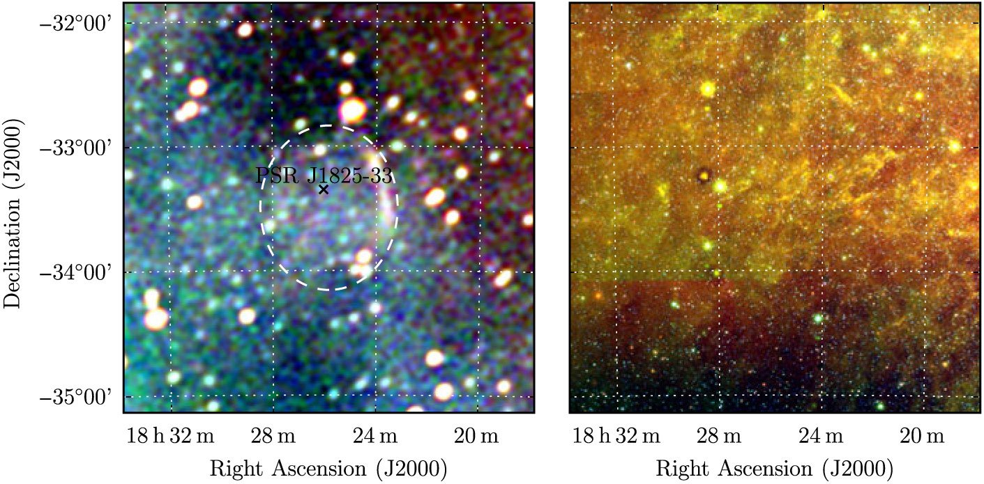
Figure 1. G 0.1−9.7 as observed by GLEAM (left) at 72–103 MHz (R), 103–134 MHz (G), and 139–170 MHz (B), and by WISE (right) at 22 μm (R), 12 μm (G), and 4.6 μm (B). The colour scales for the GLEAM RGB cube are −1.0–0.1, −0.5−0.0, and −0.2−0.1 Jy beam−1 for R, G, and B, respectively. The dashed white ellipse indicates the position of the SNR candidate, and black crosses indicate nearby pulsars.
Within the ellipse of G 0.1 − 9.7, Burke-Spolaor & Bailes (Reference Burke-Spolaor and Bailes2010) detected the rotating radio transient PSR J1825-33. They detected seven sequential pulses with a period of P = 1.27 s, implying a nulling rate of ≈97%, and were unable to estimate $\dot{P}$
; the pulsar has not subsequently been redetected. If PSR J1825-33 and G 0.1-9.7 are associated, then the pulsar’s distance of 1.24 kpc (from DM = 43 ± 2 cm−3pc) would imply a remnant diameter of 24 pc. The pulsar position uncertainty is 15 arcmin, so it would lie 3 ± 9 pc from the centre.
$\dot{P}$
; the pulsar has not subsequently been redetected. If PSR J1825-33 and G 0.1-9.7 are associated, then the pulsar’s distance of 1.24 kpc (from DM = 43 ± 2 cm−3pc) would imply a remnant diameter of 24 pc. The pulsar position uncertainty is 15 arcmin, so it would lie 3 ± 9 pc from the centre.
The western shock front may indicate initial interaction with the ISM, while the SNR continues to expand freely in the other directions. Using the measured remnant radius and assuming M ejecta = M ȯ and E = 1051 erg, Equations 1 and 2 of Paper I yield a SNR age of ≈ 1 200 yr, potentially lying within human recorded history. Alternatively, the SNR could be in the Sedov–Taylor phase; reversing Equation 4 of Paper I and assuming n H = 1 cm−3 and E = 1051 erg, we can estimate the age of the SNR as ≈9 000 yr. However, the SNR lies far off the Galactic plane and is potentially in an underdense region of the ISM, which if properly accounted for would reduce the age calculated by this method, so we could consider 9 000 yr an upper limit.
3.2. G 2.1 + 2.7
G 2.1 + 2.7 is visible as a very faint shell in both the GLEAM and E11 data (Figure 2). It is contaminated by 13 (presumably) extragalactic radio sources which are catalogued by Hurley-Walker et al. (Reference Hurley-Walker2019c). Of these, 11 sources are bright enough to fit SEDs over the GLEAM band, and subtract them from the data. The total flux density subtracted at 200 MHz is S 200MHz = 2.86 Jy, with median α = −0.93, compared to a (corrected) total remnant flux density of S 200MHz = 9 ± 1 Jy, and α = −0.19 ± 0.06. We class this remnant only as Class II.
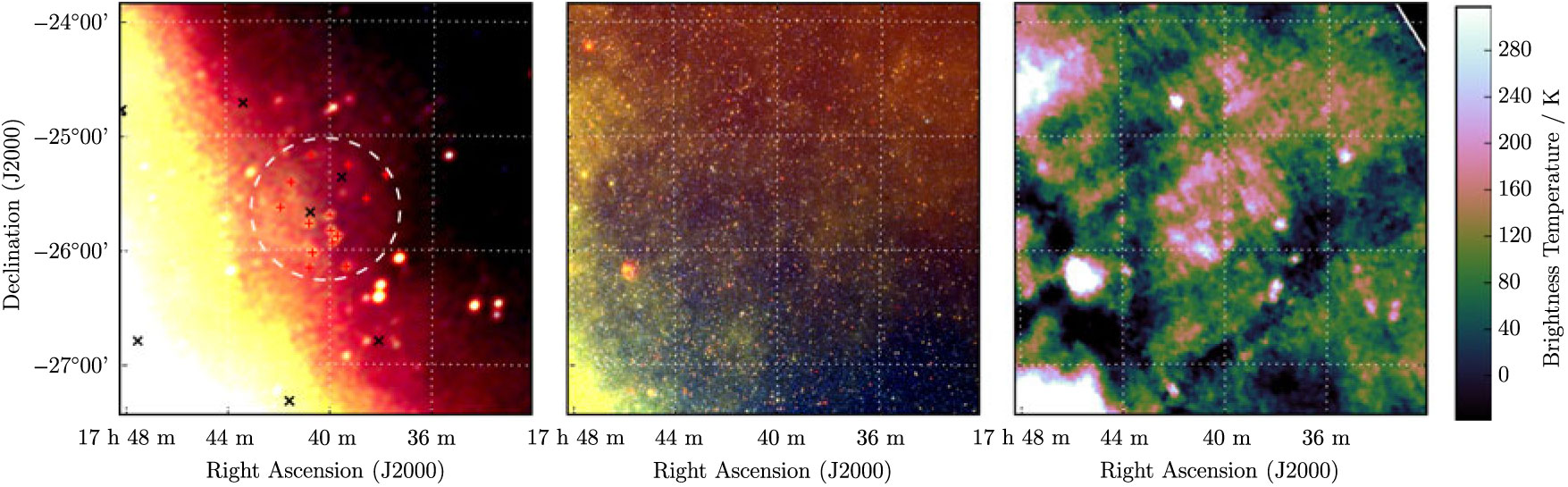
Figure 2. G 2.1 + 2.7 as observed by GLEAM (left) at 72–103 MHz (R), 103–134 MHz (G), and 139–170 MHz (B), by WISE (middle) at 22 μm (R), 12 μm (G), and 4.6 μm (B), and Effelsberg at 2.695 GHz (right). The colour scales for the GLEAM RGB cube are 0.8–2.8, 0.8–1.5, and 0.0–1.1 Jy beam−1 for R, G, and B, respectively. Annotations are as in Figure 1, and red crosses mark the positions of subtracted extragalactic radio sources (see Section 3.2).
3.3. G 7.4 + 0.3
G 7.4 + 0.3 appears as a slightly irregular ellipse with a potentially filled shell, but this is difficult to assess given its small size (≈16 arcmin) relative to the resolution of GLEAM. There is no corresponding 12- or 22-μm emission visible in the WISE image of this region (Figure 3), nor is it bright enough to be seen with E11. It has a total flux density of 2.3 ± 0.3 Jy and a non-thermal spectral index of −0.8 ± 0.2, so we conclude that it is a reasonable candidate and denote it as Class II.
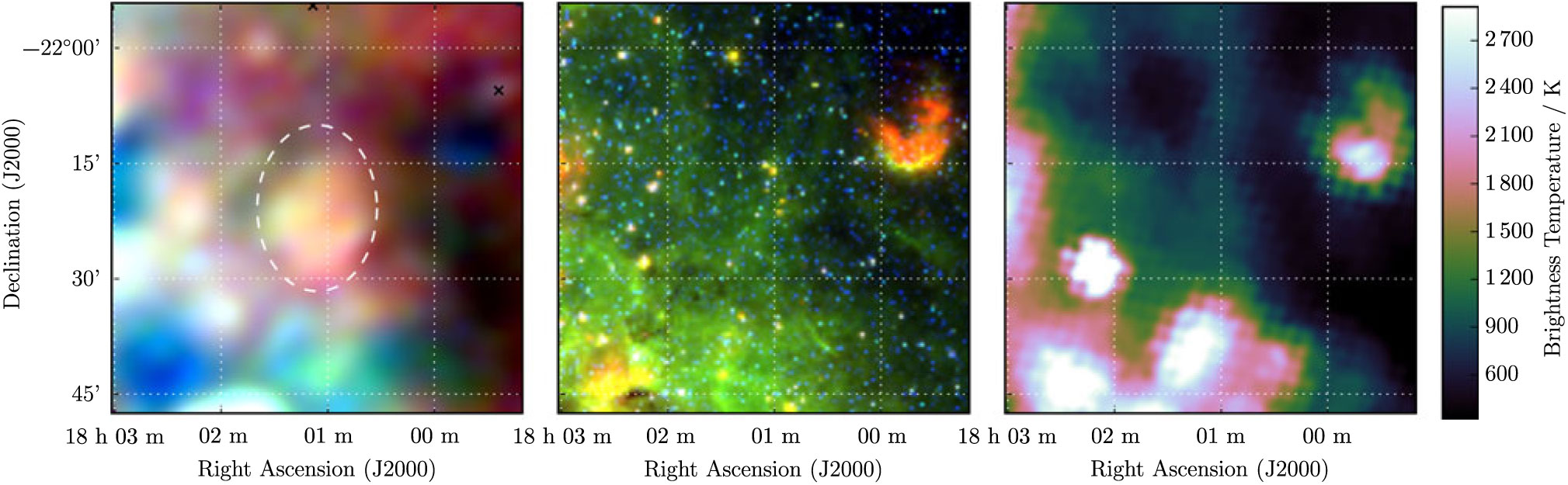
Figure 3. G 7.4 + 0.3 as observed by GLEAM (left) at 72–103 MHz (R), 103–134 MHz (G), and 139–170 MHz (B), by WISE (middle) at 22 μm (R), 12 μm (G), and 4.6 μm (B), and Effelsberg at 2.695 GHz (right). The colour scales for the GLEAM RGB cube are 4.7–6.8, 2.5–3.7, and 1.0–1.8 Jy beam−1 for R, G, and B, respectively. Annotations are as in Figure 1.
3.4. G 18.9 – 1.2
G 18.9 − 1.2 appears as a pair of distinct arcs encircling an elliptical region of increased brightness (Figure 4). Superposed is the well-studied SNR G 18.9-1.1 (Fuerst et al. Reference Fuerst, Reich, Reich, Sofue and Handa1985; the centres of the SNRs are 10 arcmin apart. We are only able to measure a total flux density for the portion of G 18.9 − 1.2 which is not confused with G 18.9 − 1.1, and find S 200MHz = 9.0 ± 0.8 Jy, and α − 1.1 ± 0.2. The spectral index of G 18.9 − 1.1 over the same band is −0.43 ± 0.04.
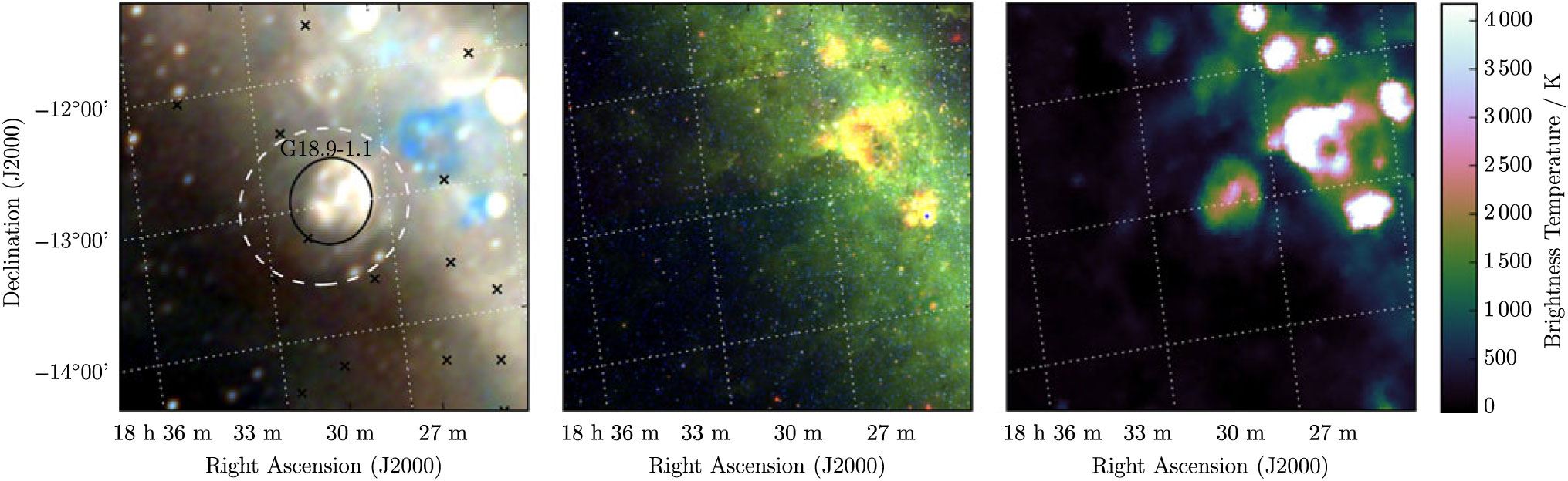
Figure 4. G 18.9−1.2 as observed by GLEAM (left) at 72–103 MHz (R), 103–134 MHz (G), and 139–170 MHz (B), by WISE (middle) at 22 μm (R), 12 μm (G), and 4.6 μm (B), and Effelsberg at 2.695 GHz (right). The colour scales for the GLEAM RGB cube are 0.7–6.7, 0.0–3.3, and −0.1–1.8 Jy beam−1 for R, G, and B, respectively. Annotations are as in Figure 1, and a black ellipse indicates a known SNR intersecting this candidate (see Section 3.4).
Potentially, the two are a single object, with G 18.9 − 1.1 the central PWNe and G 18.9 − 1.2 the original progenitor shell, and the apparent difference in central positions the result of the decreased ISM density away from the Galactic plane allowing a highly asymmetric expansion of G 18.9 − 1.2. However, the filled shell of G 18.9 − 1.1 is quite clearly delineated, and the jump in spectral indices is quite abrupt, so we postulate that the SNRs are unrelated. Given the clear shell structure and non-thermal spectrum of the SNR, we are confident in the detection and denote it as Class I.
3.5. G 19.1 – 3.1
G 19.1 − 3.1 is relatively faint and small compared to most SNRs in this work (Table 1), but does appear as a nearly complete shell with distinct edges on all but the south-east region (Figure 5). The (presumably) unrelated extragalactic radio sources GLEAM J183811-133837 and GLEAM J183646-133024 lie on the edge of the shell; care was taken to exclude them from the measurement region (Figure A.4). With the GLEAM measurements and an additional measurement from Effelsberg at 2.695 GHz, we derive S 200MHz = 2.4 ± 0.3 Jy and α = −0.6 ± 0.2. We denote the candidate Class I based solely on its intrinsic properties.
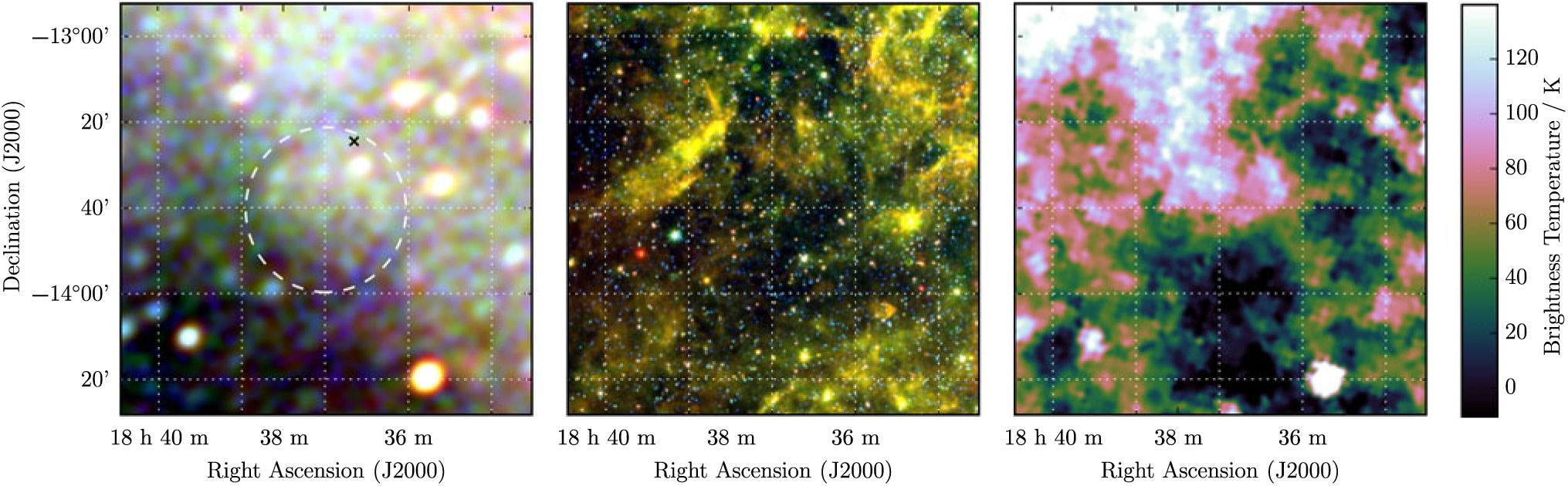
Figure 5. G 19.1−3.1 as observed by GLEAM (left) at 72–103 MHz (R), 103–134 MHz (G), and 139–170 MHz (B), by WISE (middle) at 22 μm (R), 12 μm (G), and 4.6 μm (B), and Effelsberg at 2.695 GHz (right). The colour scales for the GLEAM RGB cube are −0.1–1.3, −0.3–0.4, and −0.2–0.2 Jy beam−1 for R, G, and B, respectively. Annotations are as in Figure 1.
3.6. G 19.7 − 0.7
G 19.7 − 0.7 appears in the GLEAM data as a complete shell with thicker arcs in the north-west and south-east (Figure 6). The (presumably) unrelated extragalactic radio source GLEAM J182921-120914 lies just within the shell; care was taken to avoid including it in the measurements. Including a measurement from Effelsberg, we derive S 200MHz = 7.0 ± 0.3 Jy and α = −0.24 ± 0.05. Anderson et al. (Reference Anderson2017) also detect this SNR and name it G 19.75 − 0.69. We are confident that it is a SNR and denote it as Class I.
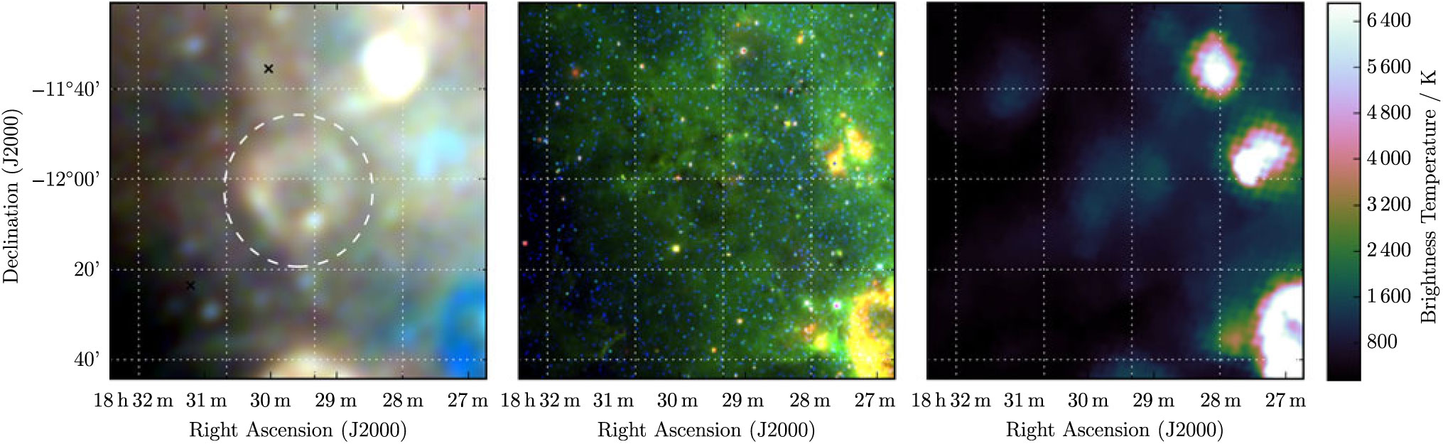
Figure 6. G 19.7−0.7 as observed by GLEAM (left) at 72–103 MHz (R), 103–134 MHz (G), and 139–170 MHz (B), by WISE (middle) at 22 μm (R), 12 μm (G), and 4.6 μm (B), and Effelsberg at 2.695 GHz (right). The colour scales for the GLEAM RGB cube are 2.7–6.8, 1.1–3.3, and 0.4–1.8 Jy beam−1 for R, G, and B, respectively. Annotations are as in Figure 1.
3.7. G 20.1 – 0.2
G 20.1 − 0.2 is visible as a partial semicircular arc bisected by the known SNR G 20.0 − 0.2. This SNR lies at a distance of 11.2 kpc (Ranasinghe & Leahy Reference Ranasinghe and Leahy2018); as G 20.1 − 0.2 has a radius 4 × larger, it is unlikely to be at the same distance, as it would be unphysically large. With H ii regions contaminating the centre of the shell, and an extremely confused background (Figure 7), we are unable to make reliable flux density measurements of the source. We denote it as merely a potential SNR candidate and Class III.
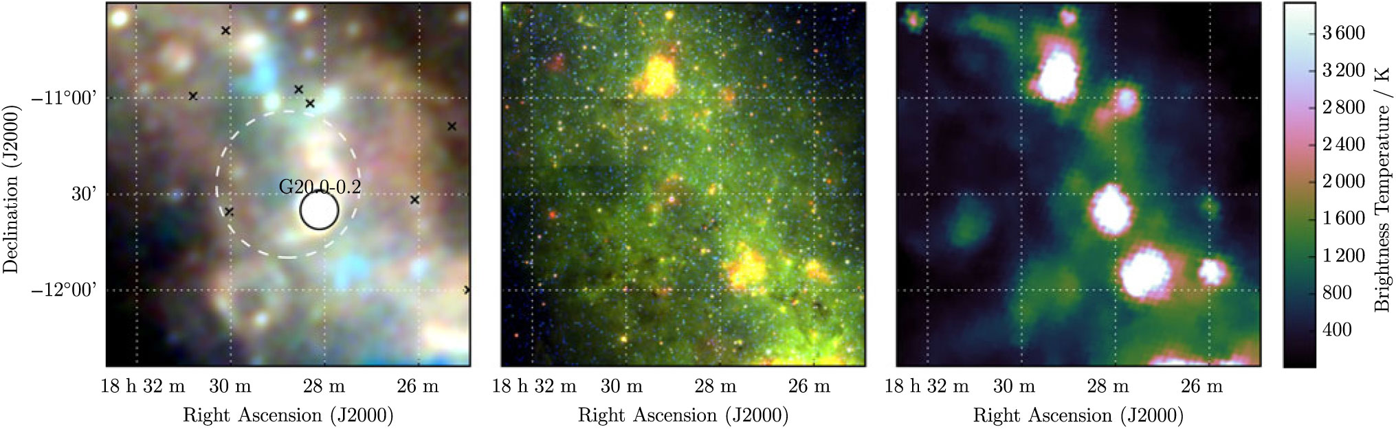
Figure 7. G 20.1−0.2 as observed by GLEAM (left) at 72–103 MHz (R), 103–134 MHz (G), and 139–170 MHz (B), by WISE (middle) at 22 μm (R), 12 μm (G), and 4.6 μm (B), and Effelsberg at 2.695 GHz (right). The colour scales for the GLEAM RGB cube are 3.3–6.7, 1.4–3.4, and 0.5–1.8 Jy beam−1 for R, G, and B, respectively. Annotations are as in Figure 1, and a black ellipse indicates a known SNR intersecting this candidate (see Section 3.7).
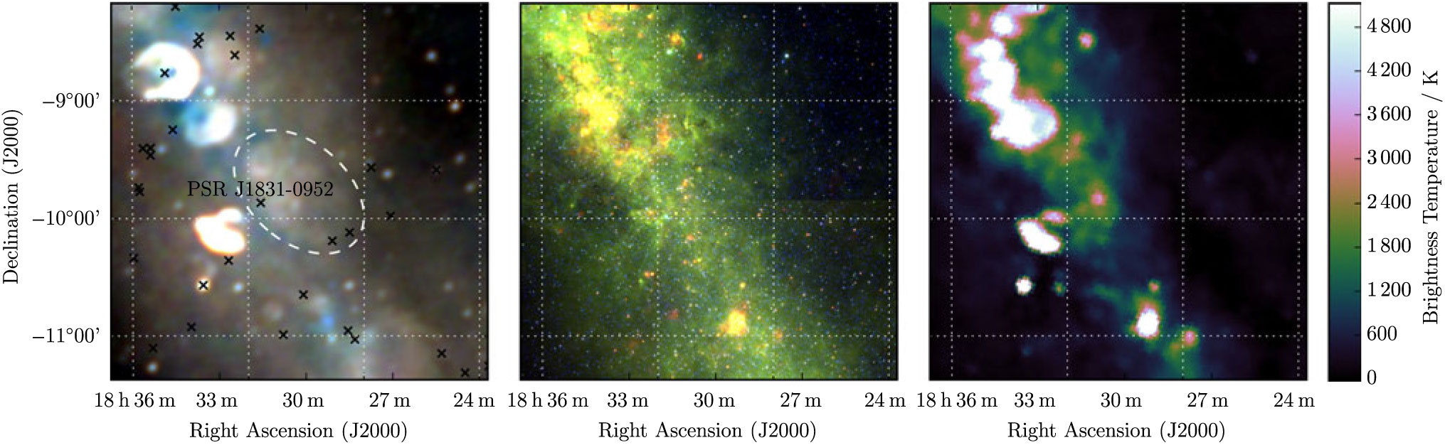
3.8. G 21.8 + 0.2
G 21.8 + 0.2 is a filled ellipse elongated in the direction of the Galactic plane (Figure 8). Despite the confusion of the region, we are able to make a reliable flux density measurement by excluding the brighter nearby SNRs from the background measurement. While not visually striking in the Effelsberg data, a measurement can be made, and we thus derive S 200MHz = 37 ± 1 Jy and α = −0.61 ± 0.05.

Figure 8. G 21.8 + 0.2 as observed by GLEAM (left) at 72–103 MHz (R), 103–134 MHz (G), and 139–170 MHz (B), by WISE (middle) at 22 μm (R), 12 μm (G), and 4.6 μm (B), and Effelsberg at 2.695 GHz (right). The colour scales for the GLEAM RGB cube are 2.2–9.4, 0.7–4.8, and 0.2–2.6 Jy beam−1 for R, G, and B, respectively. Annotations are as in Figure 1.
Due to its large size, three known pulsars lie within the ellipse; PSR J1828-1007 and PSR J1829-1011 lie to the south-west, at the edge of the ellipse, while PSR J1831-0952 lies closest, 20 arcmin south-east from the centroid of the candidate. It has P ≈ 67 ms and $\dot{P}\approx8\times10^{-15}\;{\rm s}\;{\rm s}^{-1}$
(Lorimer et al. Reference Lorimer2006), giving a characteristic age of 130 000 yr. At a distance of 3.68 kpc (derived from DM = 247 ± 5 cm−3pc), an association with the remnant would mean it has major and minor axis sizes of ≈70 × 45 pc.
$\dot{P}\approx8\times10^{-15}\;{\rm s}\;{\rm s}^{-1}$
(Lorimer et al. Reference Lorimer2006), giving a characteristic age of 130 000 yr. At a distance of 3.68 kpc (derived from DM = 247 ± 5 cm−3pc), an association with the remnant would mean it has major and minor axis sizes of ≈70 × 45 pc.
The minor axis size of 45 pc is consistent with a SNR just entering the radiative phase, where the shocked ISM is able to cool radiatively, and the SNR is driven only by internal pressure instead of the initial kinetic expansion. In this regime, the SNR radius R increases as t 2/7. The SNR clearly has an elliptical shape, implying an inhomogeneous surrounding ISM. If we make standard assumptions about the SNR energetics and ISM density, and assume adiabatic expansion up to this point, we can use Equation 4 of Paper I to derive an age estimate of 40 000–120 000 yr, for the minor and major axes, respectively. Since the SNR may have been expanding radiatively for some time, these could be underestimates. The upper end of the range is quite close to the pulsar characteristic age. The pulsar natal kick velocity would need to be 170–490 km s−1, entirely within the expected) (Verbunt et al. Reference Verbunt, Igoshev and Cator2017).
Given the large angular size of the SNR candidate (subtending 2.3 deg2), we would predict 1–2 pulsars lying inside the ellipse purely by chance, so while the astrophysics of the association is not unreasonable, caution must be advised. Regardless, the SNR candidate is strong based on its intrinsic characteristics and we therefore denote it as Class I.
3.9. G 23.1 + 0.1
G 23.1 + 0.1 is visible as a circular shell with S 200MHz = 17.3 ± 0.4 Jy beam−1 and α = −0.64 ± 0.05 (Figure 9). It is also detected in the TeV γ-rays by the High-Energy Stereoscopic System (HESS) Galactic plane survey (H.E.S.S. Collaboration et al. Reference Collaboration2018) and named HESS 1832 − 085. This interesting Class I SNR is also detected by Anderson et al. (Reference Anderson2017) and thoroughly discussed in Maxted et al. (accepted).
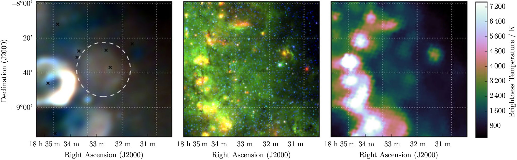
Figure 9. G 23.1 + 0.1 as observed by GLEAM (left) at 72–103 MHz (R), 103–134 MHz (G), and 139–170 MHz (B), by WISE (middle) at 22 μm (R), 12 μm (G), and 4.6 μm (B), and Effelsberg at 2.695 GHz (right). The colour scales for the GLEAM RGB cube are 3.3–14.5, 1.4–7.7, and 0.6–4.2 Jy beam−1 for R, G, and B, respectively. Annotations are as in Figure 1.
3.10. G 24.0 – 0.3
G 24.0-0.3 is very clearly visible in the GLEAM RGB image (Figure 10) and highlights the utility of this view for separating the thermal and non-thermal emission. Despite some contamination from overlapping H ii regions, we are able to obtain S 200MHz = 41 ± 1 Jy and α = −0.87 ± 0.05; the measurement from Effelsberg has a very large uncertainty so does not constrain the fit. There are hints of edge-brightening in the north-west, and the shell appears to be filled: this could either be from unresolved filamentary structure, or from a central PWNe. The high S/N of this source, clear shell-like morphology, and non-thermal spectrum, suggest strongly that it is a SNR, and we therefore denote it as Class I.
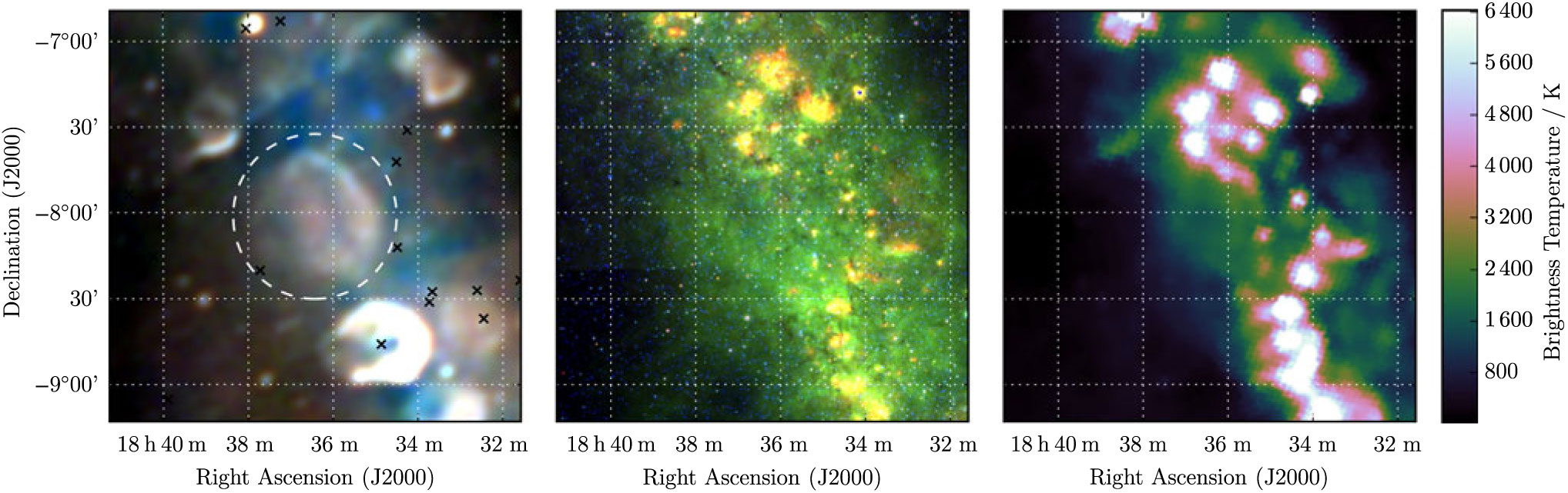
Figure 10. G 24.0−0.3 as observed by GLEAM (left) at 72–103 MHz (R), 103–134 MHz (G), and 139–170 MHz (B), by WISE (middle) at 22 μm (R), 12 μm (G), and 4.6 μm (B), and Effelsberg at 2.695 GHz (right). The colour scales for the GLEAM RGB cube are 2.6–9.2, 0.9–4.9, and 0.3–2.6 Jy beam−1 for R, G, and B, respectively. Annotations are as in Figure 1.
3.11. G 25.3 – 1.8
G 25.3 – 1.8 is spatially the largest candidate discussed in this work, covering 6.2 deg2 (Figure 11). As such it is superposed with the (presumably) unrelated extragalactic radio sources GLEAM J184249-075610, GLEAM J184309-074224, GLEAM J184440-072007, and GLEAM J184403-075954, which together comprise S 200MHz = 6.6 Jy, with median α = −0.95. Extrapolating each source across the band and subtracting them from the integrated flux density measurements, we fit to the corrected flux densities of G 25.3-1.8 and find S 200MHz = 17.0 ± 0.5 Jy and α = −0.46 ± 0.03. The SNR is clearly visible and relatively unconfused in the Effelsberg data, which is extremely useful in constraining the fit; we denote the candidate as Class I.
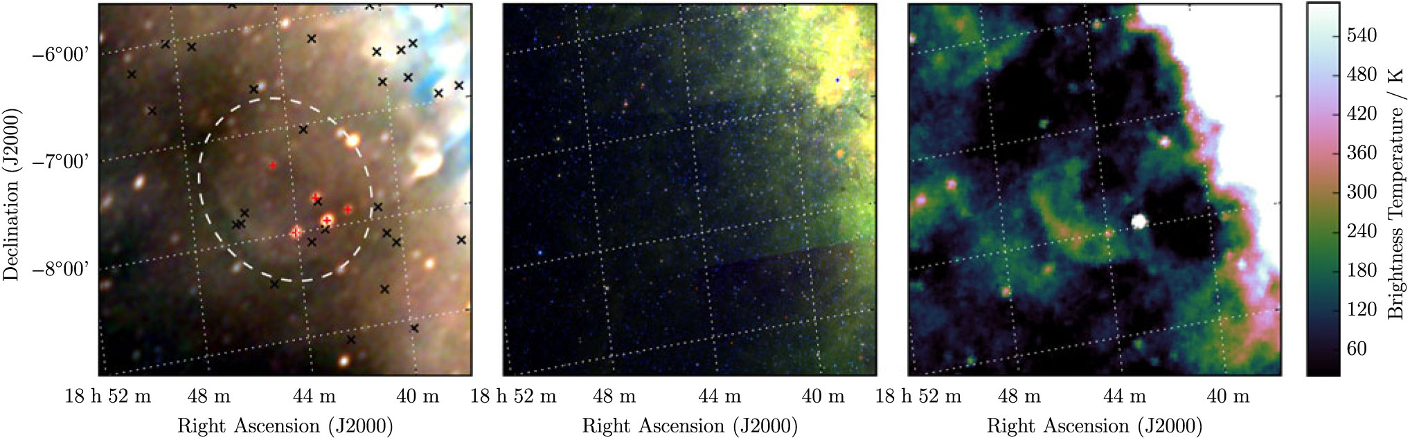
Figure 11. G 25.3−1.8 as observed by GLEAM (left) at 72–103 MHz (R), 103–134 MHz (G), and 139–170 MHz (B), by WISE (middle) at 22 μm (R), 12 μm (G), and 4.6 μm (B), and Effelsberg at 2.695 GHz (right). The colour scales for the GLEAM RGB cube are 0.8–4.9, 0.1–2.6, and 0.0–1.4 Jy beam−1 for R, G, and B, respectively. Annotations are as in Figure 1, and red crosses mark the positions of subtracted extragalactic radio sources (see Section 3.11).
3.12. G 28.3 + 0.2
G 28.3 + 0.2 is compact and circular, and almost unresolved by our observations, and entirely so by Effelsberg (Figure 12). Despite the complexity of its surroundings, we are able to derive S 200MHz = 4.2 ± 0.3 Jy and α = −0.7 ± 0.1 purely from the GLEAM measurements (Table 1). Anderson et al. (Reference Anderson2017) also detect this candidate and denote it G 28.36 + 0.21.
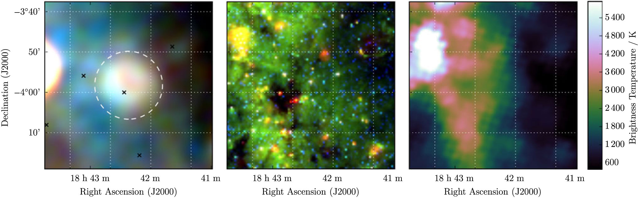
Figure 12. G 28.3 + 0.2 as observed by GLEAM (left) at 72–103 MHz (R), 103–134 MHz (G), and 139–170 MHz (B), by WISE (middle) at 22 μm (R), 12 μm (G), and 4.6 μm (B), and Effelsberg at 2.695 GHz (right). The colour scales for the GLEAM RGB cube are 3.6–6.5, 1.5–3.4, and 0.7–1.8 Jy beam−1 for R, G, and B, respectively. Annotations are as in Figure 1.
PSR B1839-04 lies very close to the centre of the candidate, but with P ≈ 1.8 s and $\dot{P}\approx5\times10^{-16}\;{\rm s}\;{\rm s}^{-1}$
(Hobbs et al. 2004b), its characteristic age of 57 Myr makes a SNR association extremely unlikely. Three other pulsars lie nearby; the youngest appears to be PSR J1841-0345, with P ≈ 204 ms and
$\dot{P}\approx5\times10^{-16}\;{\rm s}\;{\rm s}^{-1}$
(Hobbs et al. 2004b), its characteristic age of 57 Myr makes a SNR association extremely unlikely. Three other pulsars lie nearby; the youngest appears to be PSR J1841-0345, with P ≈ 204 ms and $\dot{P}\approx6\times10^{-14}\;{\rm s}\;{\rm s}^{-1}$
, yielding a characteristic age of 56 000 yr (Morris et al. Reference Morris2002). While this is typical of pulsars associated with SNRs, it is difficult to claim an association given the spatial density of both SNRs and pulsars in this region. The pulsar also lies close to a non-thermal source which is not quite resolved in the GLEAM data. Deeper, higher-resolution observations are required to determine the nature of this source and whether it might be a further candidate SNR. Returning to G 28.3 + 0.2, we are confident in its candidacy and denote it as Class I.
$\dot{P}\approx6\times10^{-14}\;{\rm s}\;{\rm s}^{-1}$
, yielding a characteristic age of 56 000 yr (Morris et al. Reference Morris2002). While this is typical of pulsars associated with SNRs, it is difficult to claim an association given the spatial density of both SNRs and pulsars in this region. The pulsar also lies close to a non-thermal source which is not quite resolved in the GLEAM data. Deeper, higher-resolution observations are required to determine the nature of this source and whether it might be a further candidate SNR. Returning to G 28.3 + 0.2, we are confident in its candidacy and denote it as Class I.
3.13. G 28.7 – 0.4
At 10 arcmin × 10 arcmin, G 28.7-0.4 is one of the smallest SNR in the sample, and just visible in the Effelsberg data (Figure 13). We thereby derive S 200MHz = 3.7 ± 0.1 Jy and α = −0.51 ± 0.06. No pulsars lie within 2 × the shell diameter so we are unable to find an association and derive any physical parameters for this source. Anderson et al. (Reference Anderson2017) also detect this object, naming it G 28.78–0.44; we are confident that it is a newly discovered SNR and denote it as Class I.
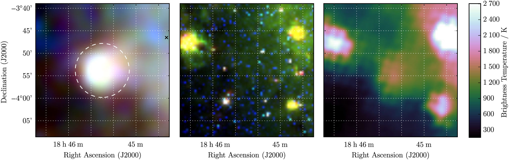
Figure 13. G 28.7−0.4 as observed by GLEAM (left) at 72–103 MHz (R), 103–134 MHz (G), and 139–170 MHz (B), by WISE (middle) at 22 μm (R), 12 μm (G), and 4.6 μm (B), and Effelsberg at 2.695 GHz (right). The colour scales for the GLEAM RGB cube are 3.5–6.3, 1.6–3.0, and 0.7–1.5 Jy beam−1 for R, G, and B, respectively. Annotations are as in Figure 1.
3.14. G 35.3 – 0.0
G 35.3–0.0 appears as an irregular elliptical region with a non-thermal spectrum (Figure 14). To its immediate east is the SNR G 35.6–0.4, and more distantly to the south is the extremely well-studied SNR G 34.7–0.4 (W44, 3C 392). On the north-east edge of the ellipse is a bright H ii region which is clearly visible in the WISE data and dominates the Effelsberg image. Care was taken to remove this, and the bright and presumably unrelated radio source to the west, from the measurement of the candidate and background flux densities. From the GLEAM data alone, we derived S 200MHz = 12.9 ± 0.4 Jy and α = −0.39 ± 0.06. Due to its unclear morphology we assign this candidate Class II, indicating our lowered confidence in a detection. Higher-resolution observations would be useful to disentangle the complexity of this region.
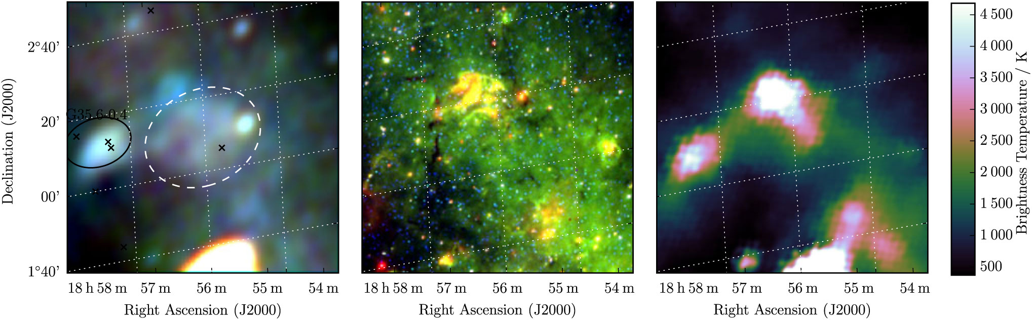
Figure 14. G 35.3−0.0 as observed by GLEAM (left) at 72–103 MHz (R), 103–134 MHz (G), and 139–170 MHz (B), by WISE (middle) at 22 μm (R), 12 μm (G), and 4.6 μm (B), and Effelsberg at 2.695 GHz (right). The colour scales for the GLEAM RGB cube are 2.9–8.7, 1.1–3.8, and 0.4–1.8 Jy beam−1 for R, G, and B, respectively. Annotations are as in Figure 1, and a black ellipse indicates a known nearby SNR (see Section 3.14).
3.15. G 230.4 + 1.2
G 230.4 + 1.2 is a very low S/N irregular ellipse in the outer Galactic plane, just barely visible in the Effelsberg data (Figure 15). It is superposed with 10 (presumably) unrelated extragalactic radio sources comprising S 200MHz = 2.7 Jy, with median α = −0.97. Fitting these sources across the GLEAM band and extrapolating them to the Effelsberg frequency, we subtract them from all measurements and obtain for the candidate S 200MHz = 3.5 ± 0.1 Jy and α = −0.60 ± 0.07.
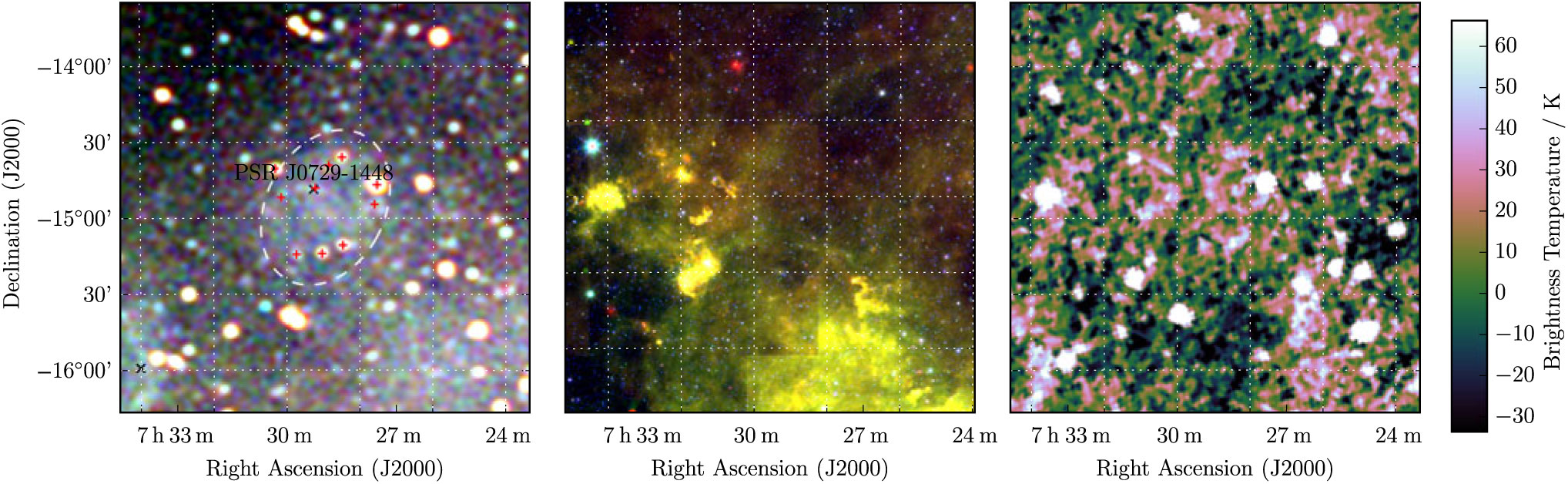
Figure 15. G 230.4 + 1.2 as observed by GLEAM (left) at 72–103 MHz (R), 103–134 MHz (G), and 139–170 MHz (B), by WISE (middle) at 22 μm (R), 12 μm (G), and 4.6 μm (B), and Effelsberg at 2.695 GHz (right). The colour scales for the GLEAM RGB cube are −0.2–0.4, −0.1–0.1, and −0.1–0.1 Jy beam−1 for R, G, and B, respectively. Annotations are as in Figure 1, and red crosses mark the positions of subtracted extragalactic radio sources (see Section 3.15)
PSR J0729-1448 lies within the ellipse, 8'.5 from the centre of the candidate; discovered in the Parkes Multibeam Survey (Morris et al. Reference Morris2002), it has P ≈ 252 ms and $\dot{P}\approx1.13\times 10^{-13}\;{\rm s}\;{\rm s}^{-1}$
, giving it a characteristic age of 35 200 yr. Its DM of 91.7 cm−3 pc (Petroff et al. Reference Petroff, Keith, Johnston, van Straten and Shannon2013) can be used to derive a distance of 2.68 kpc. If it is associated with the candidate then the ellipse is 47 × 31 pc in diameter, and the natal kick velocity of the pulsar perpendicular to the line-of-sight would be 180 km s−1, which would be fairly typical of pulsar natal velocities (Verbunt et al. Reference Verbunt, Igoshev and Cator2017).
$\dot{P}\approx1.13\times 10^{-13}\;{\rm s}\;{\rm s}^{-1}$
, giving it a characteristic age of 35 200 yr. Its DM of 91.7 cm−3 pc (Petroff et al. Reference Petroff, Keith, Johnston, van Straten and Shannon2013) can be used to derive a distance of 2.68 kpc. If it is associated with the candidate then the ellipse is 47 × 31 pc in diameter, and the natal kick velocity of the pulsar perpendicular to the line-of-sight would be 180 km s−1, which would be fairly typical of pulsar natal velocities (Verbunt et al. Reference Verbunt, Igoshev and Cator2017).
Assuming the SNR shares the pulsar’s characteristic age, it is likely to be in the Sedov–Taylor phase; for this adiabatic, self-similar expansion, we expect the SNR radius R to be proportional to its age t via Equation 4 of Paper I. After 35 200 yr, a typical SNR in this phase would therefore be ≈ 42 pc in diameter, which is very close to the value derived from the position association. Given these values, the SNR could also be transitioning to the radiative phase.
Since the chance of finding a known pulsar within this 2 deg2 candidate is < 5% for this region, we are fairly confident in this association. The low signal-to-noise of the candidate initially induces caution, but the pulsar association bolsters our confidence, allowing us to denote this candidate as Class I.
3.16. G 232.1 + 2.0
G 232.1 + 2.0 appears as an elliptical feature with dimensions ≈70' × 50' and is visible across the entire GLEAM band (Figure 16). It has poorly defined edges, potentially indicating that it is beginning to merge with the surrounding ISM. Fortunately, it is also visible in the Effelsberg 2.695 GHz data and a joint fit to the data yields S 200MHz = 7.2 ± 0.1 and α = −0.58 ± 0.02 (Table 1).
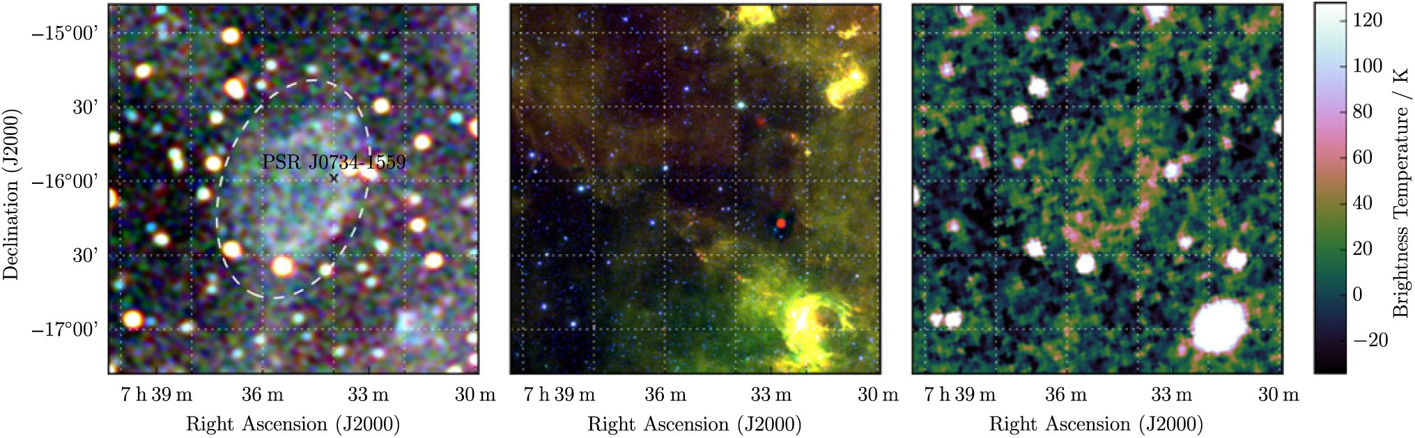
Figure 16. G 232.1 + 2.0 as observed by GLEAM (left) at 72–103 MHz (R), 103–134 MHz (G), and 139–170 MHz (B), by WISE (middle) at 22 μm (R), 12 μm (G), and 4.6 μm (B), and Effelsberg at 2.695 GHz (right). The colour scales for the GLEAM RGB cube are −0.1–0.3, −0.1–0.1, and 0.0–0.1 Jy beam−1 for R, G, and B, respectively. Annotations are as in Figure 1.
PSR J0734-1559 lies 16 arcmin from the centre of the candidate. Discovered via its γ-ray emission by Fermi-LAT, it has P ≈ 155 ms and $\dot{P}=1.25\times 10^{-14}\;{\rm s}\;{\rm s}^{-1}$
, giving it a characteristic age of 197 000 yr (Sokolova & Rubtsov Reference Sokolova and Rubtsov2016). Unfortunately, radio pulsations have not been observed from this pulsar, so its DM is not known, and no other distance estimates have yet been made.
$\dot{P}=1.25\times 10^{-14}\;{\rm s}\;{\rm s}^{-1}$
, giving it a characteristic age of 197 000 yr (Sokolova & Rubtsov Reference Sokolova and Rubtsov2016). Unfortunately, radio pulsations have not been observed from this pulsar, so its DM is not known, and no other distance estimates have yet been made.
Similarly to G 230.4 + 1.2 (Section 3.15), there is < 5% chance of a pulsar lying within the shell of the candidate purely by chance, so we are reasonably confident in the association and denote the candidate as Class I.
3.17. G 349.1 – 0.8
G 349.1–0.8 is a compact remnant which is poorly resolved by the GLEAM data and has an unclear structure in MGPS due to artefacts from nearby bright sources (Figure 17). Despite this, we are able to measure S 200MHz = 3.7 ± 0.1 Jy and α = −0.83 ± 0.07 by careful selection of the regions from which to obtain integrated flux densities and background measurements. There are no nearby known pulsars, so no physical parameters can be derived. Given the extremely unclear morphology, we denote this source as Class II.
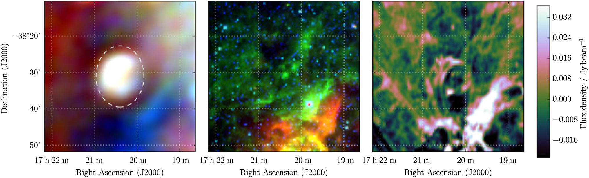
Figure 17. G 349.1−0.8 as observed by GLEAM (left) at 72–103 MHz (R), 103–134 MHz (G), and 139–170 MHz (B), by WISE (middle) at 22 μm (R), 12 μm (G), and 4.6 μm (B), and MGPS at 843 MHz (right). The colour scales for the GLEAM RGB cube are 1.6–4.5, 1.2–2.5, and 0.5–1.2 Jy beam−1 for R, G, and B, respectively.
3.18. G 350.7 + 0.6
G 350.7 + 0.6 subtends 80 arcmin × 43 arcmin, co-aligned with the Galactic plane (Figure 18). Its north-western half is superposed with a large number of H ii regions. We measure the less contaminated regions, excluding a single bright radio source to the south-west, and enclosing about half of the shell extent, while avoiding the H ii region complex and compact sources for the background measurement. From these data, we derive S 200MHz = 64 ± 1 Jy and α = −0.9 ± 0.1 across the GLEAM band, and denote the candidate as Class II.
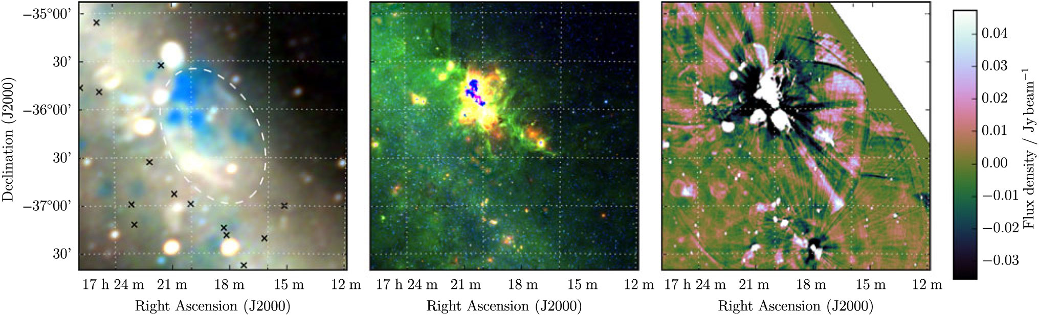
Figure 18. G 350.7 + 0.6 as observed by GLEAM (left) at 72–103 MHz (R), 103–134 MHz (G), and 139–170 MHz (B), by WISE (middle) at 22 μm (R), 12 μm (G), and 4.6 μm (B), and MGPS at 843 MHz (right). The colour scales for the GLEAM RGB cube are 1.4–8.0, 0.5–4.0, and 0.2–2.0 Jy beam−1 for R, G, and B, respectively. Annotations are as in Figure 1.
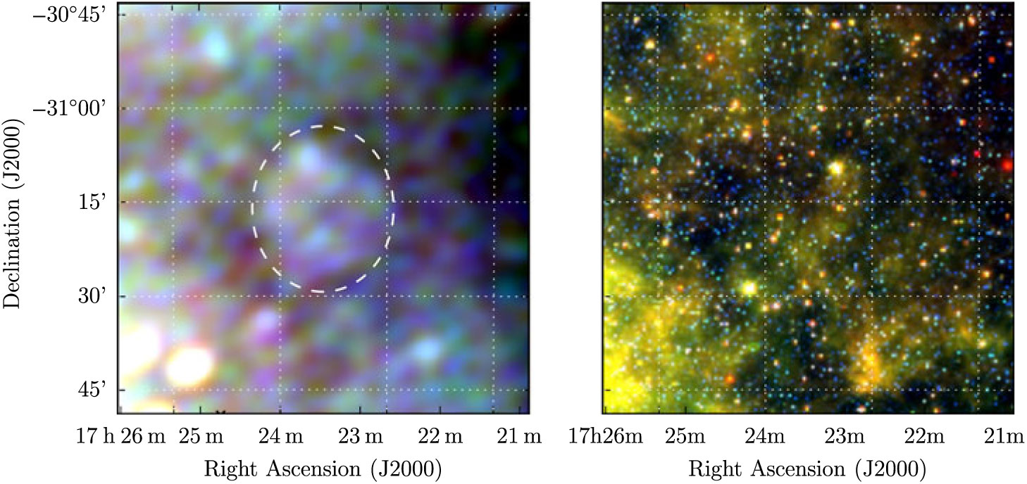
3.19. G 350.8 + 5.0
G 350.8 + 5.0 lies outside of most Galactic plane surveys and appears as a faint filled ellipsoid with no sign of edge-brightening (Figure 19). A compact source lies near the centre of the ellipsoid, appearing in the catalogue of Hurley-Walker et al. (Reference Hurley-Walker2019c) as GLEAM J170154-333857, with S 200MHz = 0.20 ± 0.02 Jy and α = −1.4 ± 0.2. Subtracting this source from our measurements of G 350.8 + 5.0, we find S 200MHz = 16.5 ± 0.4 and α = −0.27 ± 0.06. This is unusually flat spectrum for a SNR, although there is a large uncertainty on the measurement. Potentially, the steep spectrum compact source is a pulsar, and the entire SNR is a PWNe. Follow-up observations towards GLEAM J170154-333857 to search for radio or γ-ray pulsations may be useful. We denote this unusual candidate as Class II.
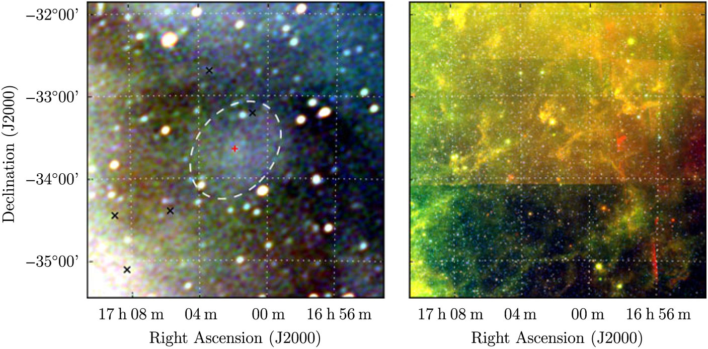
Figure 19. G 350.8 + 5.0 as observed by GLEAM (left) at 72–103 MHz (R), 103–134 MHz (G), and 139–170 MHz (B), and by WISE (right) at 22 μm (R), 12 μm (G), and 4.6 μm (B). The colour scales for the GLEAM RGB cube are 1.4–8.0, 0.5–4.0, and 0.2–2.0 Jy beam−1 for R, G, and B, respectively. Annotations are as in Figure 1.
3.20. G 351.0 – 0.6
G 351.0–0.6 appears as a partial shell half-occluded by the H ii region IRAS 17210-3646. It is more clearly resolved in the MGPS images although only the GLEAM data allow clear separation of the thermal and non-thermal components (Figure 20). For the non-occluded part of the shell, we measure S 200MHz = 0.50 ± 0.04 Jy and α = −0.64 ± 0.09 across the GLEAM and MGPS data, and class the candidate as Class II.
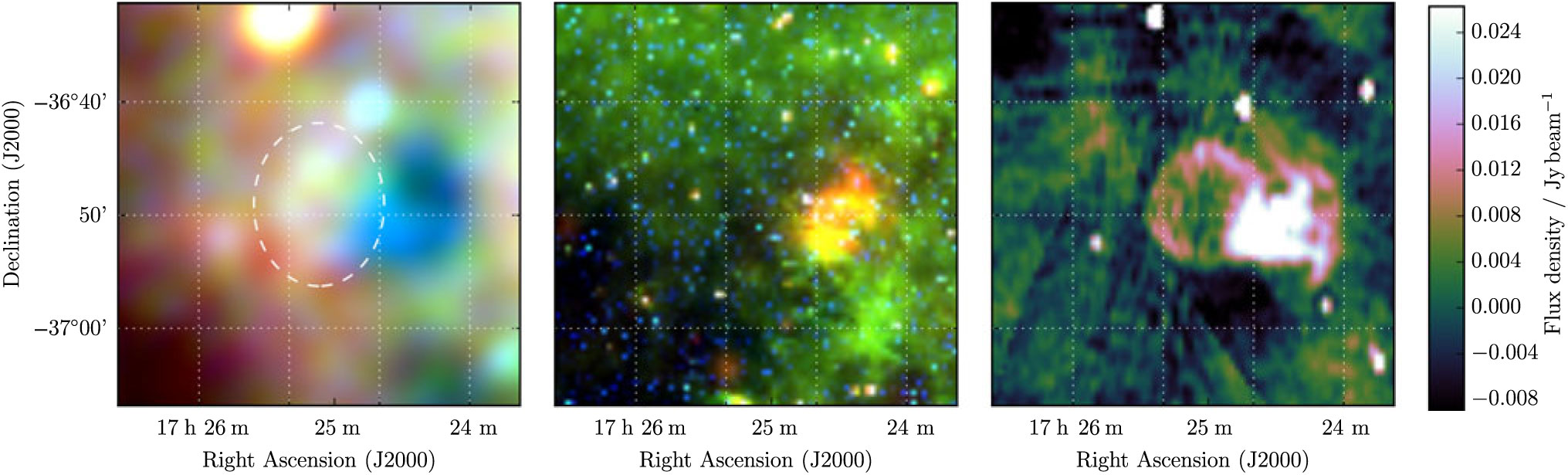
Figure 20. G 351.0−0.6 as observed by GLEAM (left) at 72–103 MHz (R), 103–134 MHz (G), and 139–170 MHz (B), by WISE (middle) at 22 μm (R), 12 μm (G), and 4.6 μm (B), and MGPS at 843 MHz (right). The colour scales for the GLEAM RGB cube are 3.7–5.3, 1.8–2.5, and 0.7–1.1 Jy beam−1 for R, G, and B, respectively. Annotations are as in Figure 1.
3.21. G 351.4 + 0.4
G 351.4 + 0.4 is spatially the smallest candidate detected in this work and is clearly visible as a full shell in MGPS (Figure 21). However, perhaps due to artefacts from the H ii complex to the west, the MGPS flux density is measured as 0.34 Jy when we would expect ≈ Jy from the GLEAM spectrum. The fit is therefore driven strongly by the GLEAM data, and we calculate S 200MHz = 3.35 ± 0.09 Jy and α = −0.42 ± 0.07 (Table 1).
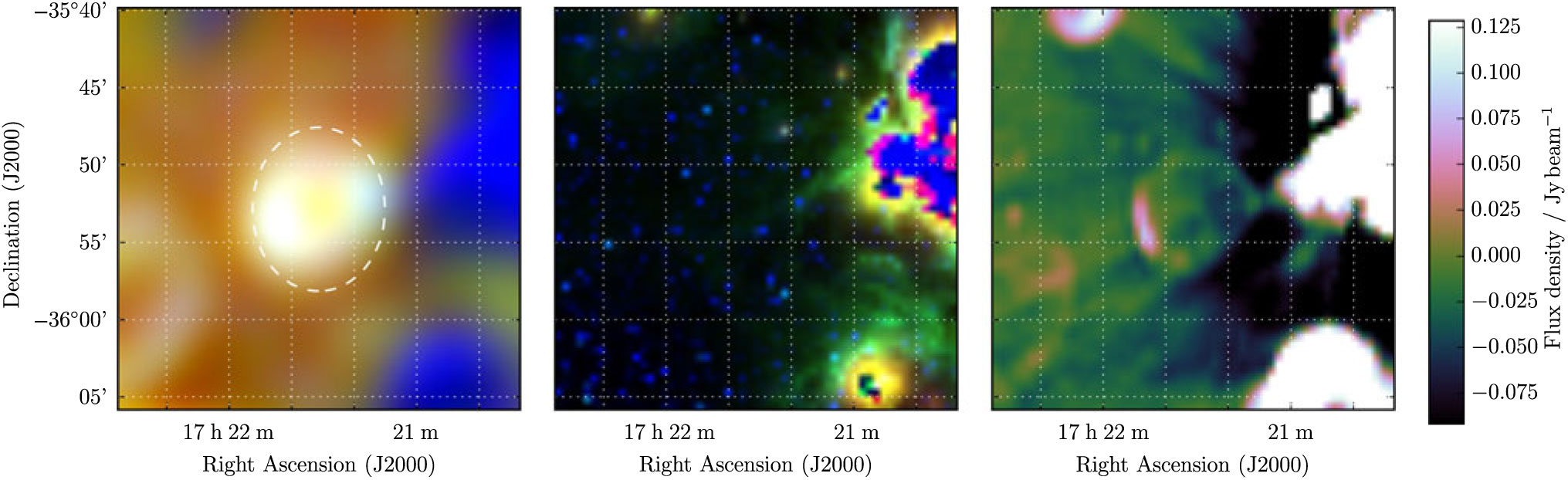
Figure 21. G 351.4 + 0.4 as observed by GLEAM (left) at 72–103 MHz (R), 103–134 MHz (G), and 139–170 MHz (B), by WISE (middle) at 22 μm (R), 12 μm (G), and 4.6 μm (B), and MGPS at 843 MHz (right). The colour scales for the GLEAM RGB cube are 1.7–9.1, 2.5–4.5, and 1.4–2.4 Jy beam−1 for R, G, and B, respectively. Annotations are as in Figure 1.
3.22. G 351.4 + 0.2
G 351.4 + 0.2 is just to the south-east of G 351.4 + 0.4 (Section 3.21) and superposed with the H ii region L89b 351.590 + 00.183 (Lockman Reference Lockman1989). Artefacts from this object reduce the reliability of the MGPS image, but the shell is still clearly visible therein (Figure 22). We use the GLEAM and MGPS measurements to determine S 200MHz = 1.8 ± 0.1 Jy and α = −0.9 ± 0.1. There are no pulsars within 2 × the diameter of the candidate so we cannot derive any physical properties, and denote the candidate as Class II, due to the confusing non-thermal emission visible to the south and east in the GLEAM image.
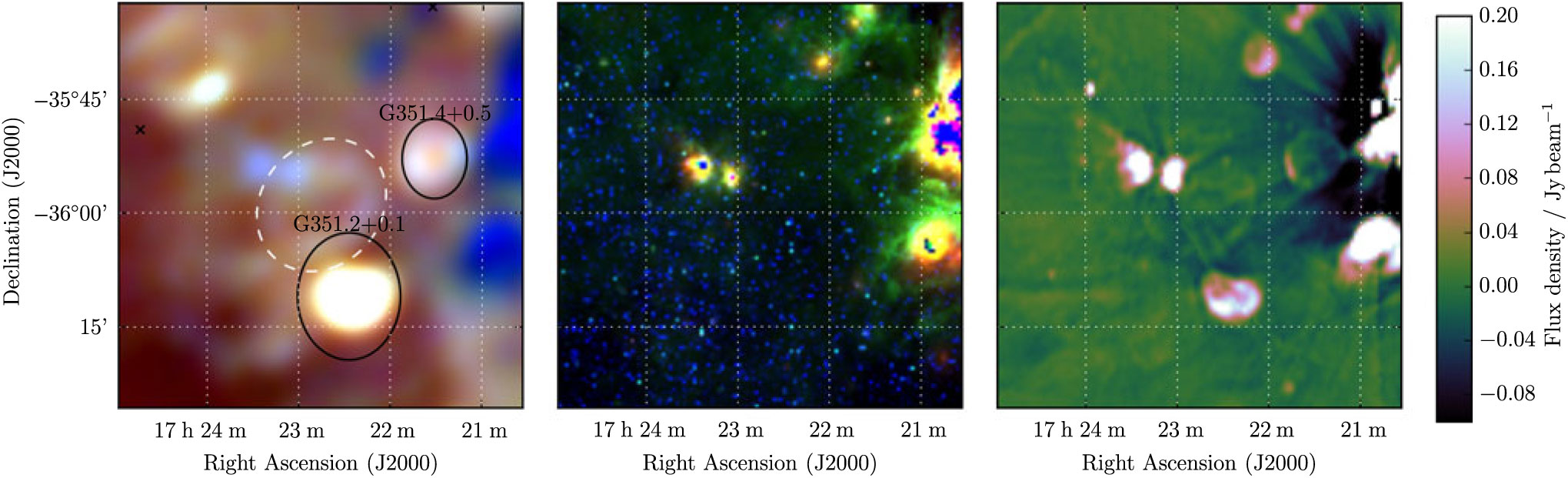
Figure 22. G 351.4 + 0.2 as observed by GLEAM (left) at 72–103 MHz (R), 103–134 MHz (G), and 139–170 MHz (B), by WISE (middle) at 22 μm (R), 12 μm (G), and 4.6 μm (B), and MGPS at 843 MHz (right). The colour scales for the GLEAM RGB cube are 2.9–9.6, 2.5–4.9, and 1.0–2.4 Jy beam−1 for R, G, and B, respectively. Annotations are as in Figure 1, and black ellipses indicate known nearby SNR (see Section 3.22). The blue region bisecting the NE of the candidate’s shell is the H ii region L89b 351.590 + 00.183.
3.23. G 351.9 + 0.1
G 351.9 + 0.1 is fairly distinct as a shell in the GLEAM images and can also be seen in MGPS (Figure 23) despite some artefacts from the nearby H ii region L89b 351.590 + 00.183 (Lockman Reference Lockman1989). Within this relatively unconfused environment, we are able to use both the GLEAM and MGPS data to derive S 200MHz = 4.1 ± 0.1 Jy and α = −0.99 ± 0.08. We are uncertain as to whether the bright source in the south-west part of the shell is associated with the SNR or not, and do not attempt to subtract it. Based on its morphology and spectrum, we assign the SNR Class II.
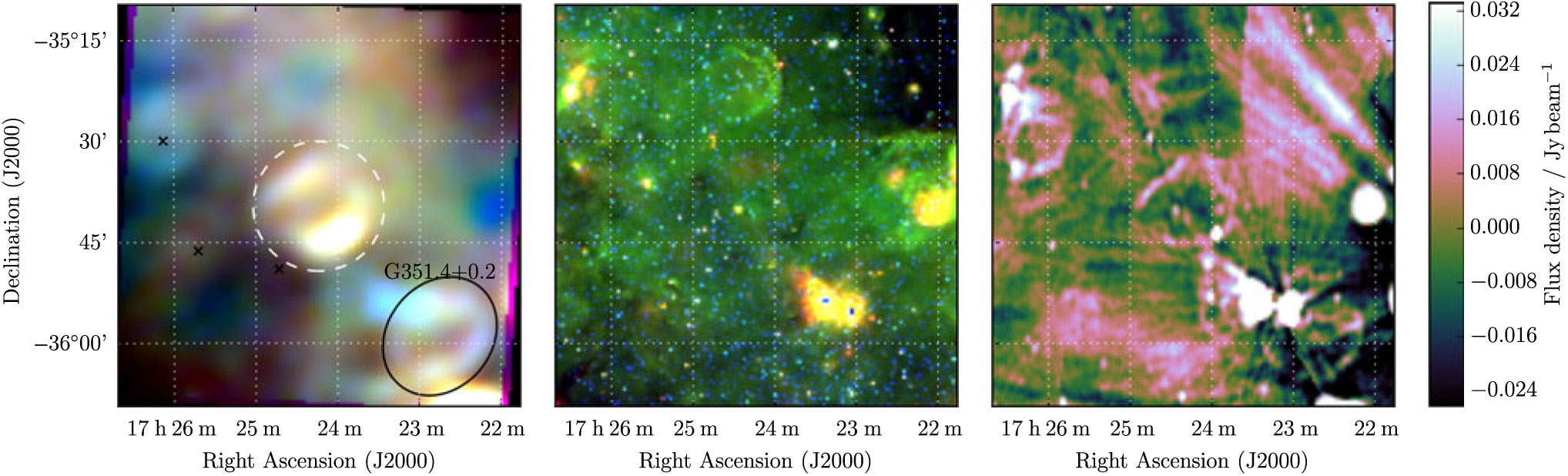
Figure 23. G 351.9 + 0.1 as observed by GLEAM (left) at 72–103 MHz (R), 103–134 MHz (G), and 139–170 MHz (B), by WISE (middle) at 22 μm (R), 12 μm (G), and 4.6 μm (B), and MGPS at 843 MHz (right). The colour scales for the GLEAM RGB cube are 5.0–8.1, 2.6–4.1, and 1.1–1.9 Jy beam−1 for R, G, and B, respectively. Annotations are as in Figure 1, and a black ellipse indicates a known nearby SNR (see Section 3.23).
3.24. G 353.0 + 0.8
G 353.0 + 0.8 is one of the most unusual candidates in the sample as it is almost completely occluded by a large H ii region complex (Figure 24). Restricting ourselves to only the westernmost edge of the shell and avoiding the H ii region during background measurement, we find S 200MHz = 16.5 ± 0.4 Jy and α = −1.0 ± 0.1 across the GLEAM band. There are some brighter spots towards the edges of the shell where it appears to be in contact with the H ii region, but at this low resolution any physical interpretation is impossible. Given how unusual this object is, we denote it as Class III.
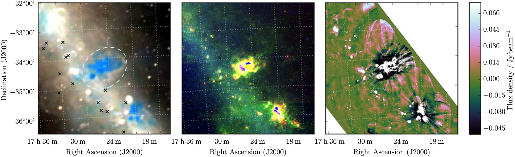
Figure 24. G 353.0 + 0.8 as observed by GLEAM (left) at 72–103 MHz (R), 103–134 MHz (G), and 139–170 MHz (B), by WISE (middle) at 22 μm (R), 12 μm (G), and 4.6 μm (B), and MGPS at 843 MHz (right). The colour scales for the GLEAM RGB cube are 1.1–8.2, 0.3–4.3, and 0.1–2.1 Jy beam−1 for R, G, and B, respectively.
3.25. G 355.4 + 2.7
G 355.4 + 2.7 appears as an irregular elliptical patch of increased brightness (Figure 25), with a non-thermal spectrum; from the GLEAM measurements alone, we derive S 200MHz = 1.5 ± 0.2 Jy and α = −0.8 ± 0.2. With no pulsar association and no coverage from other Galactic plane surveys, we cannot comment further on this candidate, but suggest that its morphology and spectrum are enough to denote it as Class I.

Figure 25. G 355.4 + 2.7 as observed by GLEAM (left) at 72–103 MHz (R), 103–134 MHz (G), and 139–170 MHz (B), and by WISE (right) at 22 μm (R), 12 μm (G), and 4.6 μm (B). The colour scales for the GLEAM RGB cube are 2.0–3.6, 0.8–1.4, and 0.2–0.5 Jy beam−1 for R, G, and B, respectively.
3.26. G 356.5 – 1.9
G 356.5–1.9 is shown as a faint ellipse of uniform brightness, appearing brighter at higher Galacitic latitude (SE on Figure 26) due to the gradient of Galactic synchrotron background. It is east of the known SNR G 356.3–1.5 (Gray Reference Gray1994) and is superposed to the north-west with a roughly triangular non-thermal radio source. It is unclear whether this source is associated with the infrared source IRAS 17412-3236, which is potentially an infrared bubble (MGE 356.7168-01.7246 in Mizuno et al. Reference Mizuno2010), although it has an unusual bipolar structure in the radio (Figure 4 of Ingallinera et al. Reference Ingallinera2016); or, with the SNR candidate IGR J17448–3232 detected by Tomsick et al. (Reference Tomsick, Chaty, Rodriguez, Walter and Kaaret2009) using the Chandra X-ray Observatory at 0.3–1.0 keV; or, with some other chance radio emission along the line-of-sight.
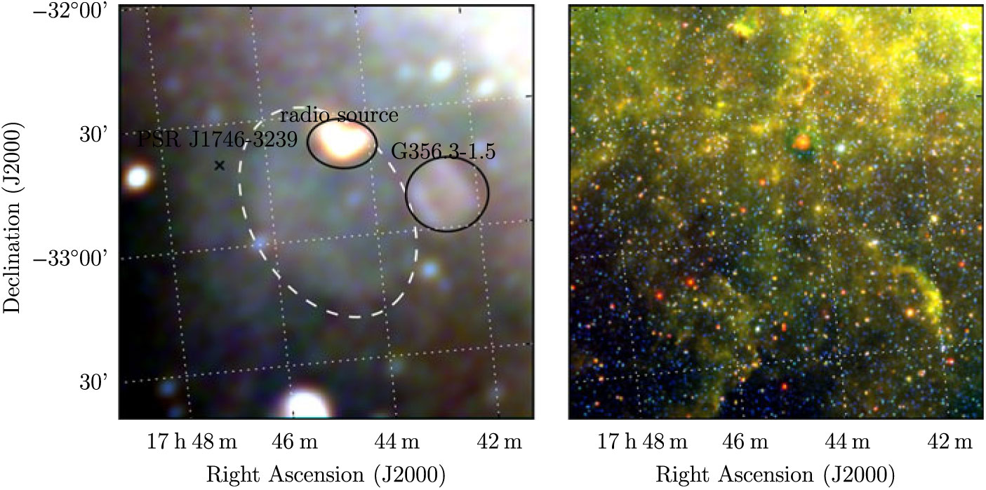
Figure 26. G 356.5−1.9 as observed by GLEAM (left) at 72–103 MHz (R), 103–134 MHz (G), and 139–170 MHz (B), and by WISE (right) at 22 μm (R), 12 μm (G), and 4.6 μm (B). The colour scales for the GLEAM RGB cube are 1.9–6.1, 0.6–2.7, and 0.2–1.1 Jy beam−1 for R, G, and B, respectively. Annotations are as in Figure 1, and black ellipses indicate known nearby objects (see Section 3.26).
In any case, care was taken to avoid this object when calculating integrated flux densities for G 356.5–1.9. A fit over the flux density measurements yielded S 200MHz = 14.9 ± 0.3 Jy and α = −0.71 ± 0.05; while the surface brightness is low, the large size of the candidate yields a high total S/N.
PSR J1746-3239 lies just outside of G 356.5–1.9; with P ≈ 200 ms and $\dot{P}\approx6.6\times10^{-15}$
it has a characteristic age of 482 000 yr, which is on the high side for a potential association. The pulsar was discovered by Pletsch et al. (Reference Pletsch2012) via its γ-ray emission; despite an extensive campaign, the authors did not detect a radio counterpart, so its DM is unknown and a distance estimate cannot be made. In any case, G 356.5–1.9 is denoted Class I due to its elliptical morphology and non-thermal spectrum.
$\dot{P}\approx6.6\times10^{-15}$
it has a characteristic age of 482 000 yr, which is on the high side for a potential association. The pulsar was discovered by Pletsch et al. (Reference Pletsch2012) via its γ-ray emission; despite an extensive campaign, the authors did not detect a radio counterpart, so its DM is unknown and a distance estimate cannot be made. In any case, G 356.5–1.9 is denoted Class I due to its elliptical morphology and non-thermal spectrum.
3.27. G 358.3 – 0.7
G 358.3–0.7 is one of the faintest SNR in the sample and appears to be contaminated with thermal emission in the centre of the shell. It is somewhat confused to the north-east with the known SNRs G 359.0–0.9 and G 358.5–0.9 (Gray Reference Gray1994), as well as other non-thermal filaments in the region which may indicate further unknown SNRs (Figure 27). Restricting ourselves to the south-west section of the shell which is clear enough to measure, we find S 200MHz = 21.8 ± 0.3 Jy and α = −0.8 ± 0.1 across the GLEAM band.
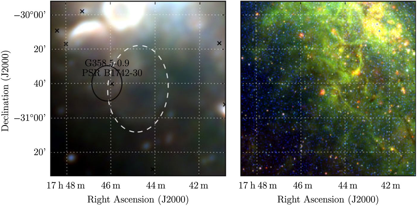
Figure 27. G 358.3–0.7 as observed by GLEAM (left) at 72–103 MHz (R), 103–134 MHz (G), and 139–170 MHz (B), and by WISE (right) at 22 μm (R), 12 μm (G), and 4.6 μm (B). The colour scales for the GLEAM RGB cube are 4.6–22.2, 1.8–11.6, and 0.7–5.4 Jy beam−1 for R, G, and B, respectively. Annotations are as in Figure 1, and black ellipses indicate known nearby objects (see Section 3.27).
The nearby pulsar PSR B1742-30 (Komesaroff et al. Reference Komesaroff, Ables, Cooke, Hamilton and McCulloch1973) has P ≈ 370 ms and $\dot{P}\approx10^{-14}\;{\rm s}\;{\rm s}^{-1}$
, yielding a characteristic age of 550 000 yr (Li et al. Reference Li, Wang, Yuan, Wang, Hobbs, Lentati and Manchester2016). The DM measured by Hobbs et al. (Reference Hobbs2004a) is 88.373 cm−3pc and this yields a distance estimate of 2.64 kpcFootnote b. An association would imply that the candidate has diameter 26 × 32 pc, placing it in the Sedov–Taylor phase of adiabatic expansion. Reversing Equation 4 of Paper I and making standard assumptions about the SNR energy and ISM density, we can use the SNR radius to predict the age, finding t ≈ 10 000 − 18 000 yr, not very consistent with the pulsar characteristic age.
$\dot{P}\approx10^{-14}\;{\rm s}\;{\rm s}^{-1}$
, yielding a characteristic age of 550 000 yr (Li et al. Reference Li, Wang, Yuan, Wang, Hobbs, Lentati and Manchester2016). The DM measured by Hobbs et al. (Reference Hobbs2004a) is 88.373 cm−3pc and this yields a distance estimate of 2.64 kpcFootnote b. An association would imply that the candidate has diameter 26 × 32 pc, placing it in the Sedov–Taylor phase of adiabatic expansion. Reversing Equation 4 of Paper I and making standard assumptions about the SNR energy and ISM density, we can use the SNR radius to predict the age, finding t ≈ 10 000 − 18 000 yr, not very consistent with the pulsar characteristic age.
Li et al. (Reference Li, Wang, Yuan, Wang, Hobbs, Lentati and Manchester2016) also measure a range of values for the proper motion of the pulsar, with $\dot{\alpha}=11.9 \pm 16 - 24 \pm 6\; {\rm mas}\; {\rm yr}^{-1}$
and
$\dot{\alpha}=11.9 \pm 16 - 24 \pm 6\; {\rm mas}\; {\rm yr}^{-1}$
and $\dot{\delta}=30 \pm 11 - 75 \pm 49 \;{\rm mas}\; {\rm yr}^{-1}$
depending on the derivation method used. Ignoring the listed uncertainties and using purely the range of values, this gives possible pulsar motion directions with angles varying from 10–40° (CCW from north), the latter being marginally consistent with the geometry shown in Figure 27. Using Li et al.’s best estimate of the total proper motion of 33 ± 11 mas yr−1 (but not their distance estimate), we calculate that the pulsar would need to have travelled for ≈ 27 000 yr to arrive at its current location, again inconsistent with the pulsar characteristic age, although not far from the predicted expansion age, especially given the uncertainties.
$\dot{\delta}=30 \pm 11 - 75 \pm 49 \;{\rm mas}\; {\rm yr}^{-1}$
depending on the derivation method used. Ignoring the listed uncertainties and using purely the range of values, this gives possible pulsar motion directions with angles varying from 10–40° (CCW from north), the latter being marginally consistent with the geometry shown in Figure 27. Using Li et al.’s best estimate of the total proper motion of 33 ± 11 mas yr−1 (but not their distance estimate), we calculate that the pulsar would need to have travelled for ≈ 27 000 yr to arrive at its current location, again inconsistent with the pulsar characteristic age, although not far from the predicted expansion age, especially given the uncertainties.
We conclude that the association is somewhat unlikely, especially given the complexity of the region; a better estimate of the pulsar’s proper motion would be necessary to use this as evidence of association. The candidate itself is denoted as Class III.
4. Discussion
We compare the newly detected SNRs with the G17 catalogue of known SNRs. Figure 28 shows histograms of the Galactic longitude of known and new SNRs. The sensitivity of GLEAM drops towards high l, and we find no new SNRs beyond l > 40°, as image artefacts make interpretation more difficult. We find no new SNRs in the range 3° < l < 18°, in part due to confusion from the amount of Galactic emission, but perhaps also because this is a region that has already been extensively searched for SNRs. Examining Figure 29, we find that lowered confusion at high |b| makes detection of faint shells much easier, and the wide field-of-view of the instrument automatically yields a large survey area. These high-latitude SNRs are likely to be nearby (< 2 kpc) and make superb probes of their local ISM, which is otherwise difficult to examine. Sixty per cent of the candidates subtend areas larger than 0.2 deg2 on the sky, compared to < 25% of previously detected SNRs (Figure 31).
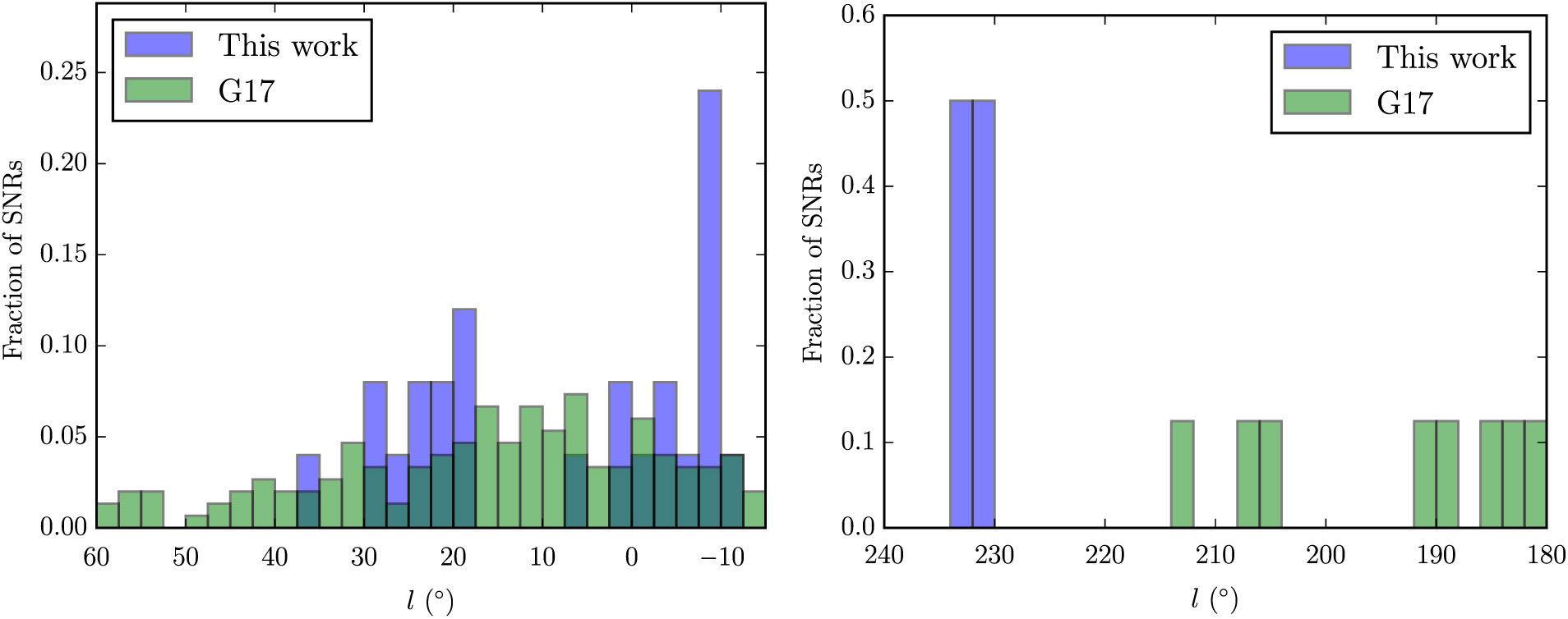
Figure 28. Histograms of Galactic longitude l, comparing the SNR candidates discovered in this work with the known SNRs catalogued by G17, normalised by height, for each panel. The left panel the range 345° < l < 60° and the right panel shows 180° < l < 240°.
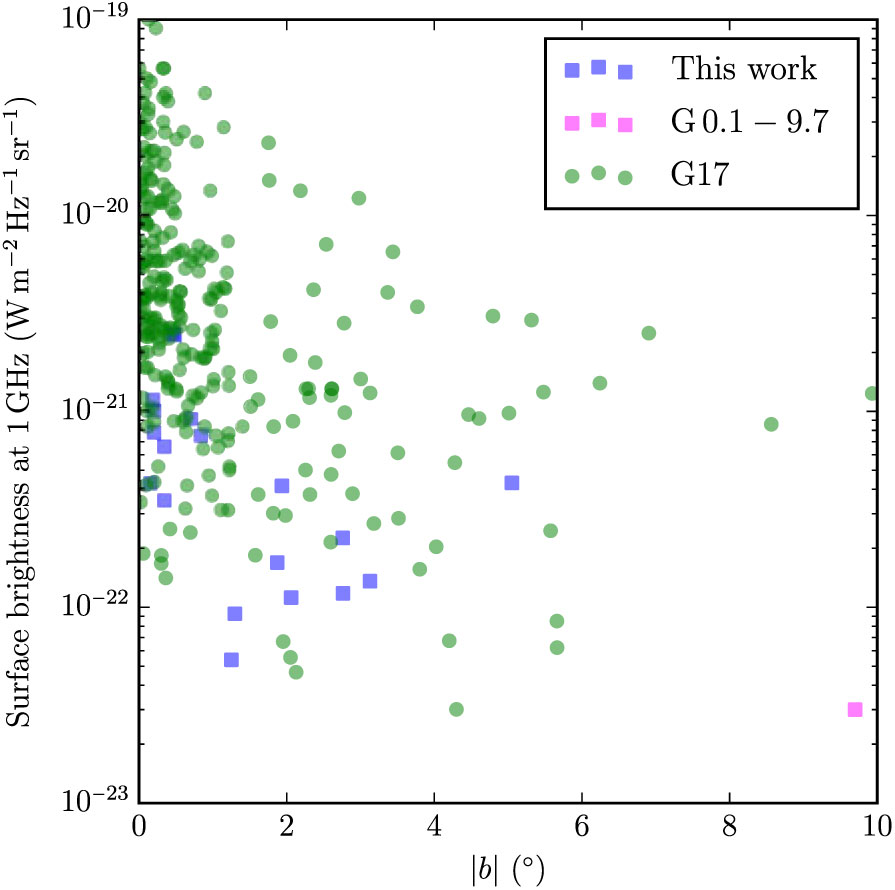
Figure 29. Surface brightness of SNR candidates with respect to absolute Galactic latitude b, for the SNR candidates discovered in this work and the known SNRs catalogued by G17. The surface brightness of G 0.1–9.7 was derived by measuring the brightness of a central region of the ellipse at 72 MHz and extrapolating to 1 GHz (see Section 3.1).
We discover two new candidates in a region previously empty of SNRs: G 230.4 + 1.2 and G 232.1 + 2.0, each with low 1 GHz-surface brightnesses of ≈ 10−22 W m−2 Hz−1 sr−1, amongst the faintest ever detected. A population of low surface brightness objects at 180° < l < 240° would be easy to explore with more integration time due to the very low confusion levels, but clearly high sensitivity levels are required. This longitude range has no massive star formation regions, potentially indicating these SNR formed from relatively old B-type stars which have migrated from their stellar nurseries.
Figure 30 shows histograms of the 1 GHz flux density and surface brightness of the candidates, compared to known SNRs. The total flux densities are often not significantly lower than the known population, but it is clear from the second panel that they tend to have much lower brightness. Figure 31 shows that the population also have steeper spectra and subtend larger areas. We may be seeing SNRs with very little active energy injection, with an older population of electrons, resulting in steeper synchrotron spectra. The fact that the survey is at low frequencies and is searching previously observed areas does bias our results towards finding steeper spectrum objects. Looking at Table 1, there does not seem to be any significant correlation of spectral index with morphology.
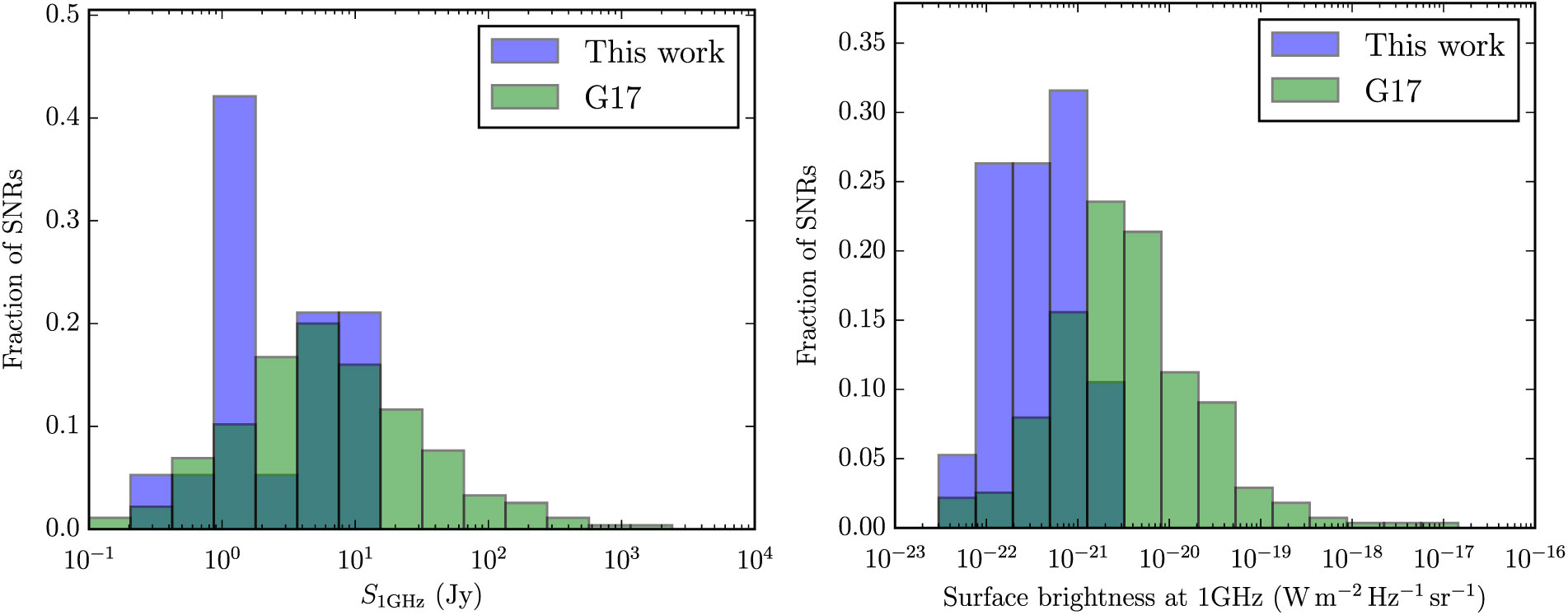
Figure 30. Histograms comparing the SNR candidates discovered in this work with the known SNRs catalogued by G17, normalised by height, for each panel. The left panel shows the 1 GHz flux density and the right panel shows the surface brightness. For the candidates discovered in this work, partial objects are excluded, and the 1 GHz values were derived from the fitted values of S 200MHz and α shown in Table 1.
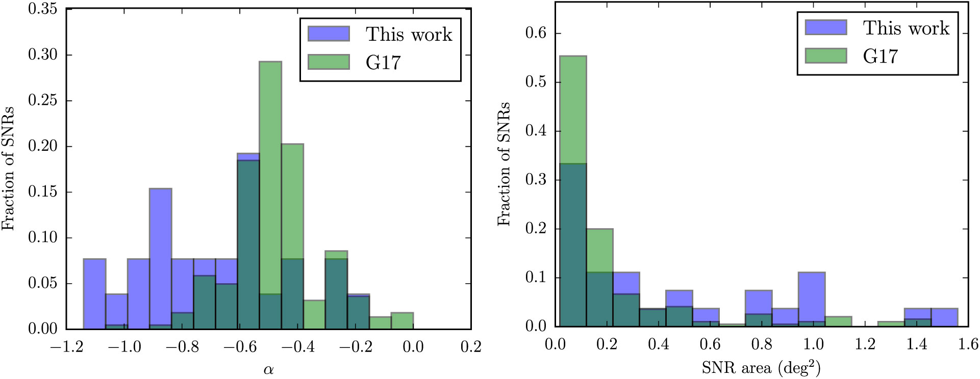
Figure 31. Histograms comparing the SNR candidates discovered in this work with the known SNRs catalogued by G17, normalised by height, for each panel. The left panel shows the spectral index α and the right panel shows the subtended area in square degrees. Partial candidates were not excluded and their extrapolated areas were used based on their major and minor axes (Table 1).
We did not detect any of our candidates in the relatively shallow Röntgensatellit All-Sky Survey (RASS) data, and there were no chance alignments with pointed observations using the 30 arcsec × 30 arcsec fields-of-view of XMM-Newton and Chandra. The upcoming all-sky X-ray extended ROentgen Survey with an Imaging Telescope Array (eROSITA; Cappelluti et al. Reference Cappelluti2011) will be 20 – 30 × more sensitive than RASS. Measurement of, or limits on, the X-ray emission of these candidates will allow us to more accurately determine their ages and energetics, which can then confirm or deny the hypothesis that the electron populations in the steep spectrum sources are older.
Edge-brightening in some of the SNRs may indicate strong interactions with the local ISM. At these locations, we expect to find molecular clouds hosting prominent CO emission, (see e.g. Moriguchi et al. Reference Moriguchi, Tamura, Tawara, Sasago, Yamaoka, Onishi and Fukui2005; Maxted et al. Reference Maxted2012). Upcoming surveys such as The Mopra Southern Galactic Plane CO Survey (Braiding et al. Reference Braiding2018) will be able to detect these clouds and provide SNR distance estimates, as well as probing the interactions between the clouds and shock fronts. Older supernova shocks are more likely to host broad-line spectral line emission, revealing complex velocity gradients across the ISM. Using H i emission and absorption to probe near the SNRs will map the local dynamics of the ISM, possible on ≈ 30 arcsec scales using the upcoming high-sensitivity Galactic Australian Square Kilometer Array Pathfinder survey (Dickey et al. Reference Dickey2013).
The discovery of 27 new SNRs increases the known number by ≈10%. The Galactic longitude range 240° < l < 345° hosts many massive star-forming regions and is likely to host at least as many candidate SNRs again (Johnston-Hollitt in prep). While our survey method is biased towards detecting steep spectrum objects, this population was not previously known to exist, indicating that these objects may make up a large fraction of the SNRs yet to be found. The other large fraction yet to be discovered is likely to be SNRs of small apparent size, at large distances, and thus will only be found by high-resolution surveys able to probe through the Galactic disc (e.g. the 76 new candidate SNRs discovered by Anderson et al. Reference Anderson2017).
Further discoveries at low Galactic latitudes will not be gained by integrating for longer with low-resolution surveys, due to confusion. The upcoming GLEAM-eXtended (GLEAM-X; Hurley-Walker in prep) survey will cover the entire southern sky at 1 arcmin resolution and the same wide bandwidth as GLEAM, which will considerably reduce confusion and allow better morphological characterisation of compact candidates. At high Galactic latitudes, extragalactic source confusion introduces a noise floor at ≈ 1 mJy beam−1 at 200 MHz (≈ 7 × 10⁻²⁴ W m−2 Hz−1 sr−1 extrapolated to 1 GHz with α = −0.5). This is ≈ 7 × the RMS noise of the extragalactic GLEAM survey so further low-resolution integration may yet yield further candidates, but with diminishing returns. A low-frequency telescope configuration including both short and long baselines yielding sub-arcmin resolution and sensitivity to 1°–10° structures would be best placed to yield further candidates.
5. Conclusions
We have detected 27 new SNRs using a new data release of the GLEAM survey from the MWA telescope, including the lowest surface brightness SNR ever detected, G 0.1–9.7. Our method uses spectral fitting to the radio continuum to derive spectral indices for 26/27 candidates, and our low-frequency observations probe a steeper spectrum population than previously discovered, as well as SNR of large angular extent. None of the candidates have coincident WISE mid-IR emission, further showing that the emission is non-thermal.
We make the first detection of two SNRs in the Galactic longitude range 220°–240°: follow-up observations of the pulsars at the heart of these SNRs would allow derivation of physical parameters, increasing our knowledge of these SNRs far from known star-forming regions.
For our low-resolution survey, confusion at low Galactic latitudes makes new detections challenging. However, the wide bandwidth of the MWA allows us to discriminate thermal and non-thermal emission, uncovering large SNRs in complex regions, previously missed by high-frequency narrowband surveys. A combination of higher-resolution data from the upgraded MWA and the inclusion of all GLEAM data should yield further detections of as-yet unknown SNRs.
Acknowledgements
We thank Gavin Rowell, Loren Anderson, and Jennifer West for useful feedback on the draft manuscript, and the anonymous referee for their helpful comments which improved the paper. This scientific work makes use of the Murchison Radio-astronomy Observatory, operated by CSIRO. We acknowledge the Wajarri Yamatji people as the traditional owners of the Observatory site. Support for the operation of the MWA is provided by the Australian Government (NCRIS), under a contract to Curtin University administered by Astronomy Australia Limited. We acknowledge the Pawsey Supercomputing Centre which is supported by the Western Australian and Australian Governments. We acknowledge the work and support of the developers of the following python packages: Astropy (The Astropy Collaboration et al. 2013), Numpy (van der Walt et al. Reference van der Walt, Colbert and Varoquaux2011), and Scipy (Jones et al. Reference Jones, Oliphant and Peterson2001). We also made extensive use of the visualisation and analysis packages DS9Footnote c and Topcat (Taylor Reference Taylor, Systems, Shopbell, Britton and Ebert2005). This work was compiled in the very useful free online LaTeX editor Overleaf. This publication makes use of data products from the Wide-field Infrared Survey Explorer, which is a joint project of the University of California, Los Angeles, and the Jet Propulsion Laboratory/California Institute of Technology, funded by the National Aeronautics and Space Administration.
Appendix A. Regions used to determine SNR flux densities
These plots follow the format of Figure 1 of Paper I, indicating where the polygons were drawn in Polygon_Flux to measure SNRs. The top two panels of each figure show the GLEAM 170–231 MHz images; the lower two panels show the RGB cube formed from the 72–103 MHz (R), 103–134 MHz (G), and 139–170 MHz (B) images. As described in Section 2.3 of Paper I, the annotations on the right two panels consist of: white polygons to indicate the area to be integrated in order to measure the SNR flux density; blue dashed lines to indicate regions excluded from any background measurement; the light shaded area to show the region that is used to measure the background, which is then subtracted from the final flux density measurement. Figures proceed in the same order as in Section 3. SNRs for which no GLEAM spectrum was extracted are excluded from this list.
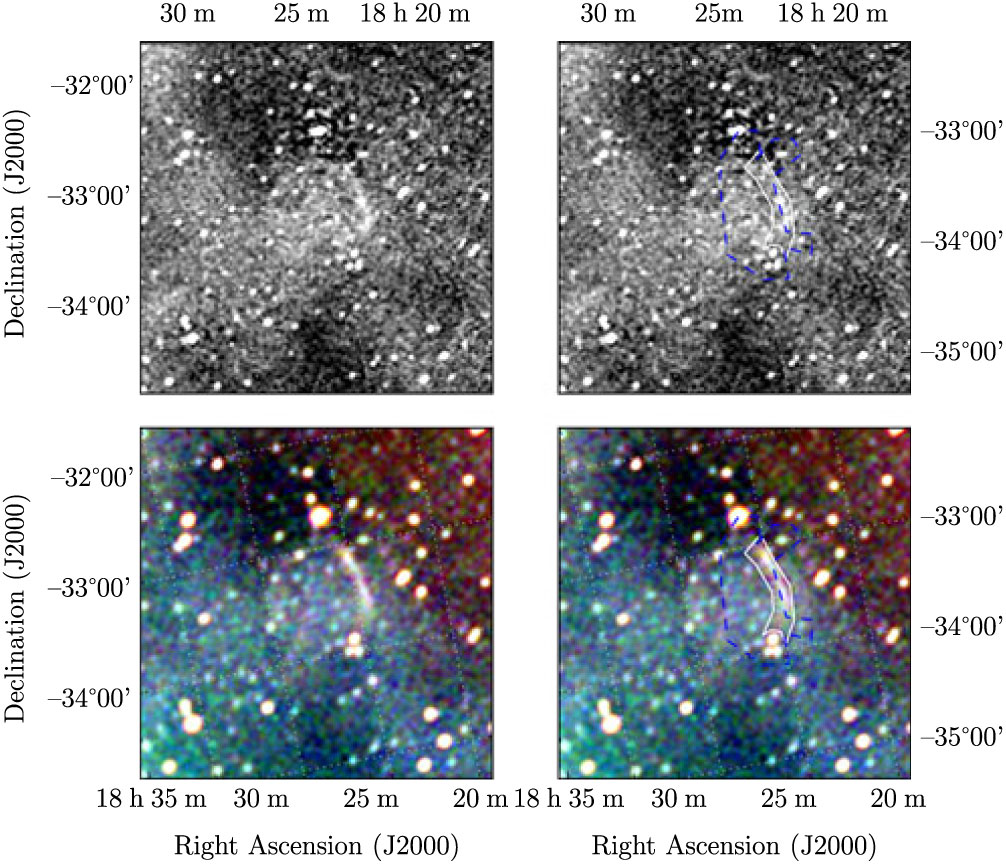
Figure A.1. Polygons drawn over GLEAM images to measure source and background flux densities for G0.1 − 9.7.
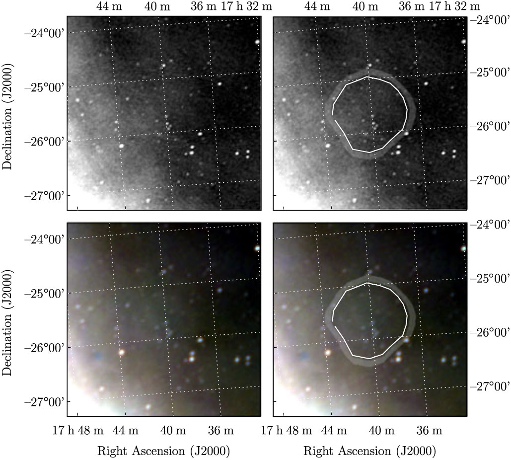
Figure A.2. Polygons drawn over GLEAM images to measure source and background flux densities for G2.1 + 2.7.
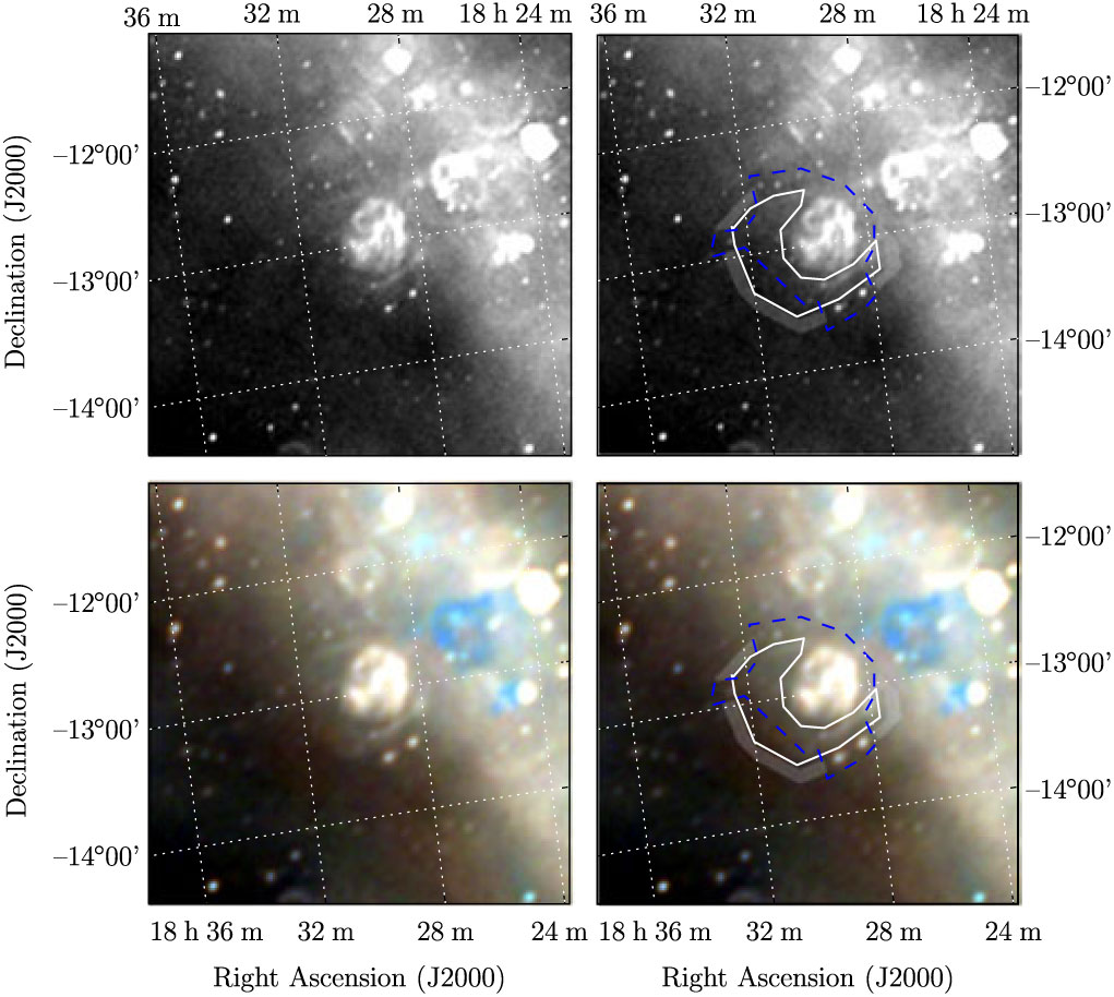
Figure A.3. Polygons drawn over GLEAM images to measure source and background flux densities for G18.9 − 1.2.
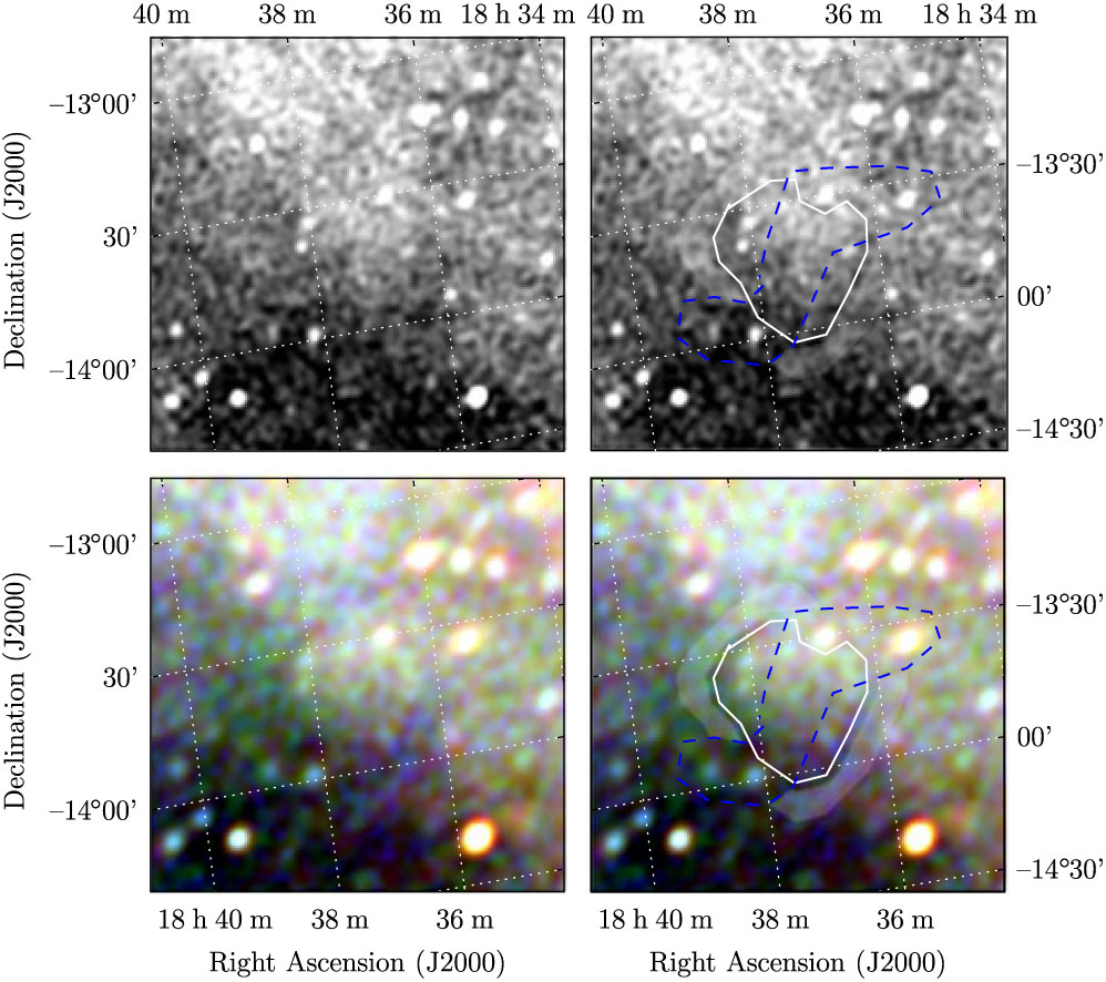
Figure A.4. Polygons drawn over GLEAM images to measure source and background flux densities for G19.1 − 3.1.
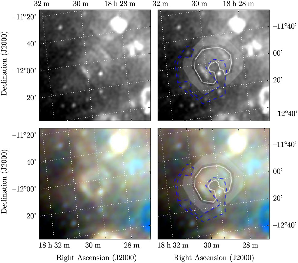
Figure A.5. Polygons drawn over GLEAM images to measure source and background flux densities for G19.7 − 0.7.
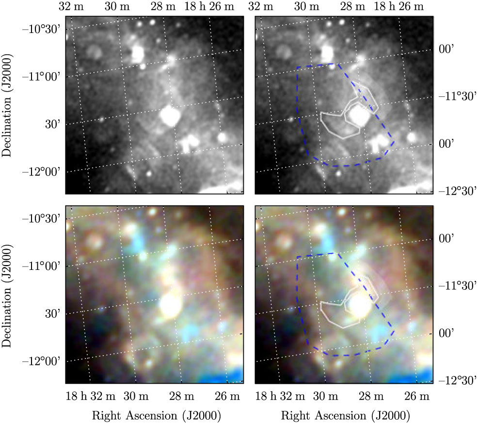
Figure A.6. Polygons drawn over GLEAM images to measure source and background flux densities for G20.1 − 0.2.
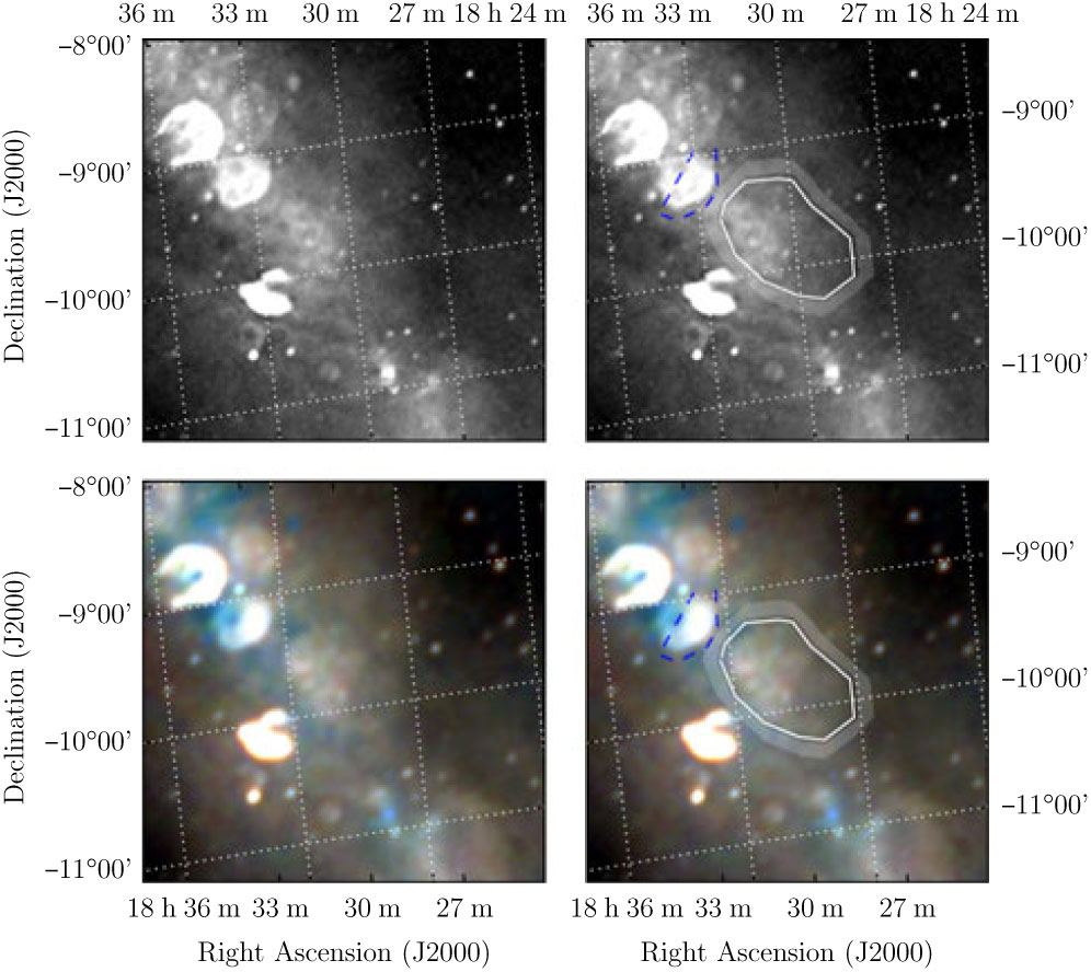
Figure A.7. Polygons drawn over GLEAM images to measure source and background flux densities for G21.8 + 0.2.
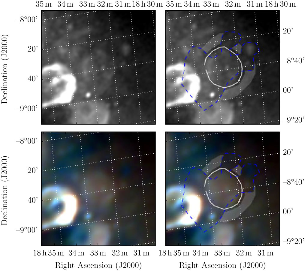
Figure A.8. Polygons drawn over GLEAM images to measure source and background flux densities for G23.1 + 0.1.
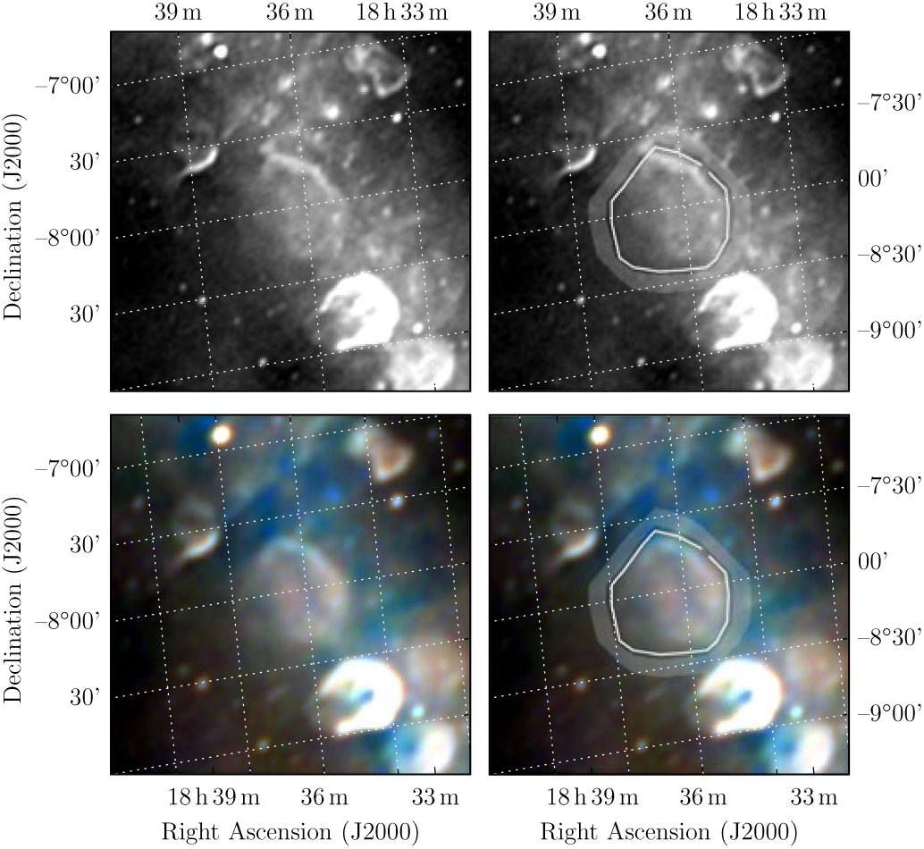
Figure A.9. Polygons drawn over GLEAM images to measure source and background flux densities for G24.0 − 0.3.
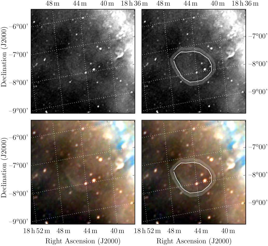
Figure A.10. Polygons drawn over GLEAM images to measure source and background flux densities for G25.3 − 1.8.
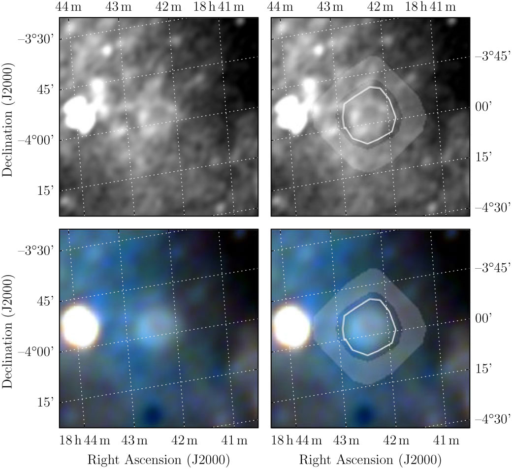
Figure A.11. Polygons drawn over GLEAM images to measure source and background flux densities for G28.3 + 0.2.
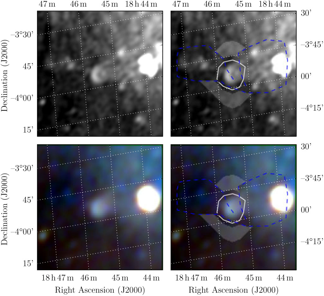
Figure A.12. Polygons drawn over GLEAM images to measure source and background flux densities for G28.7 − 0.4.
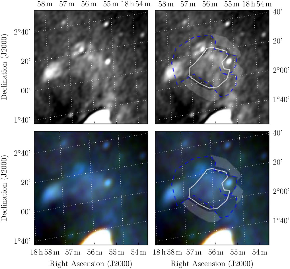
Figure A.13. Polygons drawn over GLEAM images to measure source and background flux densities for G35.3 − 0.0.
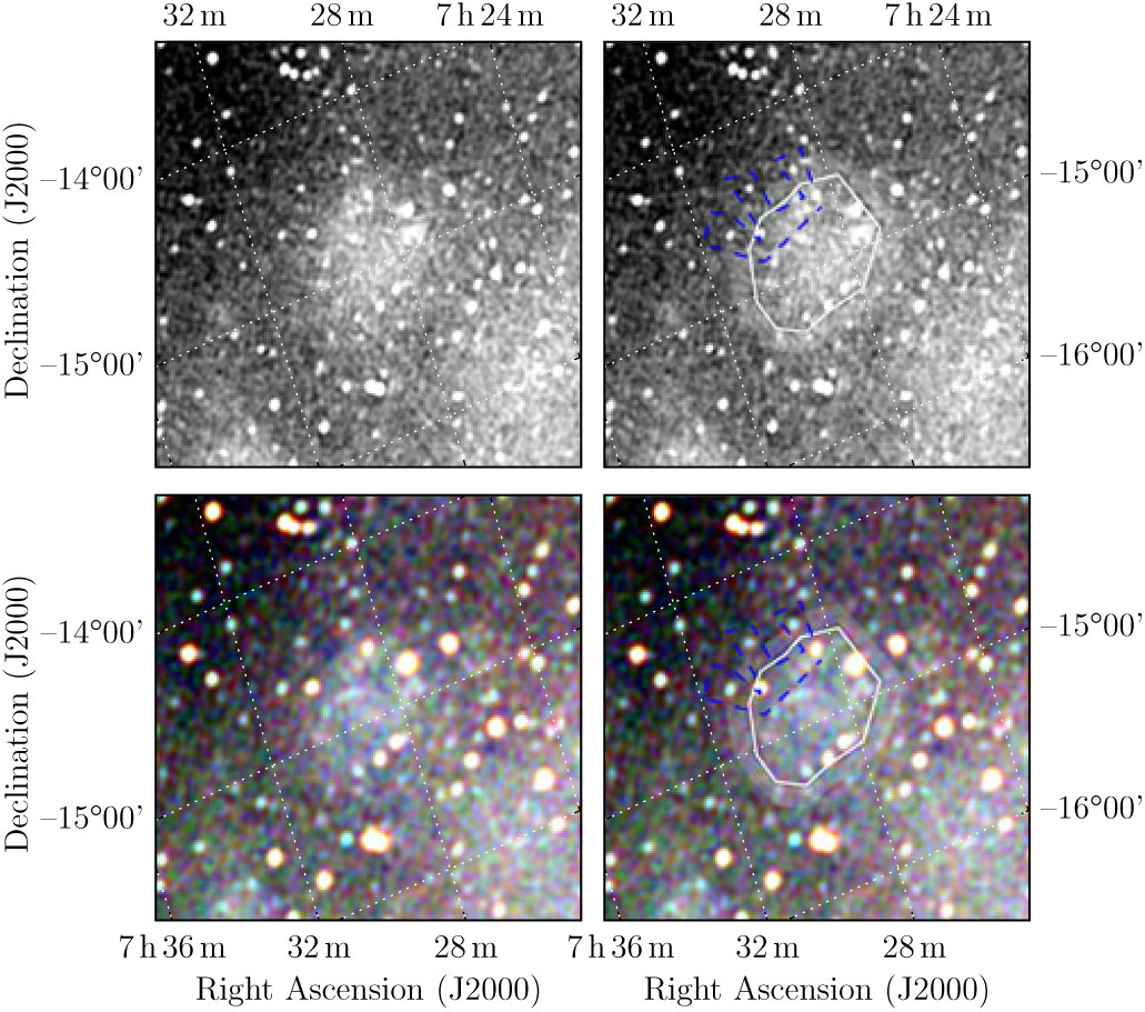
Figure A.14. Polygons drawn over GLEAM images to measure source and background flux densities for G230.4 + 1.2.
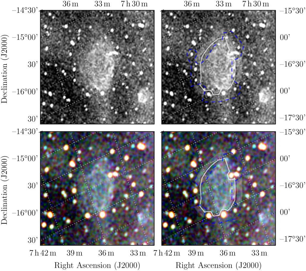
Figure A.15. Polygons drawn over GLEAM images to measure source and background flux densities for G232.1 + 2.0.
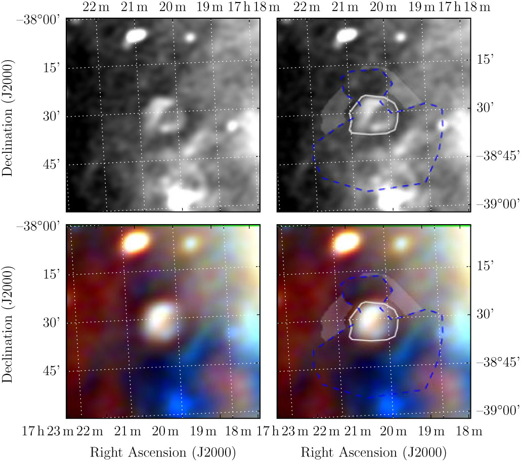
Figure A.16. Polygons drawn over GLEAM images to measure source and background flux densities for G349.1 − 0.8.
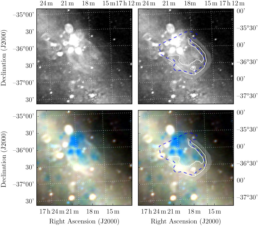
Figure A.17. Polygons drawn over GLEAM images to measure source and background flux densities for G350.7 + 0.6.
Appendix B. Spectra
The spectra of the measured SNR using the backgrounding and flux-summing technique described in Sections 2.3 and 2.4 of Paper I, for the 26 objects for which spectra could be derived. The left panels show flux density against frequency with linear axes while the right panels show the same data in log. (It is useful to include both when analysing the data as a log plot does not render negative data points, which occur for faint SNRs). The black points show the (background-subtracted) SNR flux density measurements, the red points show the measured background, and the blue curve shows a linear fit to the log-log data (i.e. S νa ∝ ν α). The fitted value of α is shown at the top right of each plot.
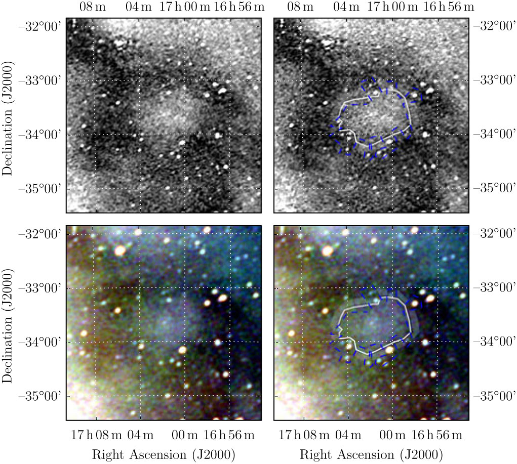
Figure B.1. Polygons drawn over GLEAM images to measure source and background flux densities for G350.8 + 5.0.
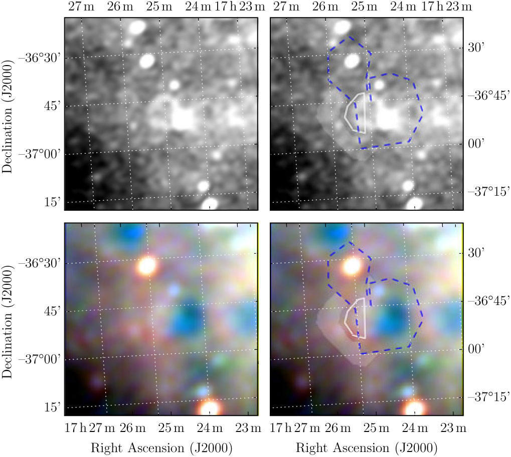
Figure B.2. Polygons drawn over GLEAM images to measure source and background flux densities for G351.0 − 0.6.
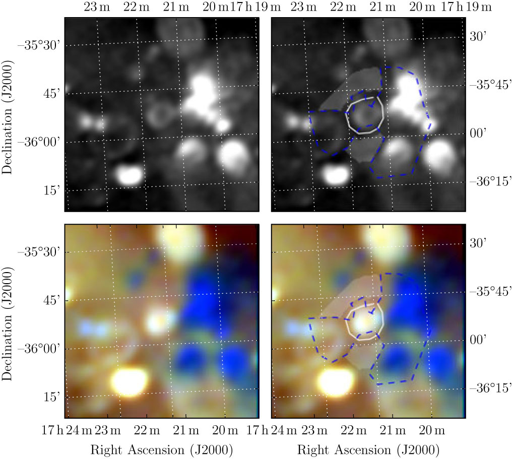
Figure B.3. Polygons drawn over GLEAM images to measure source and background flux densities for G351.4 + 0.4.
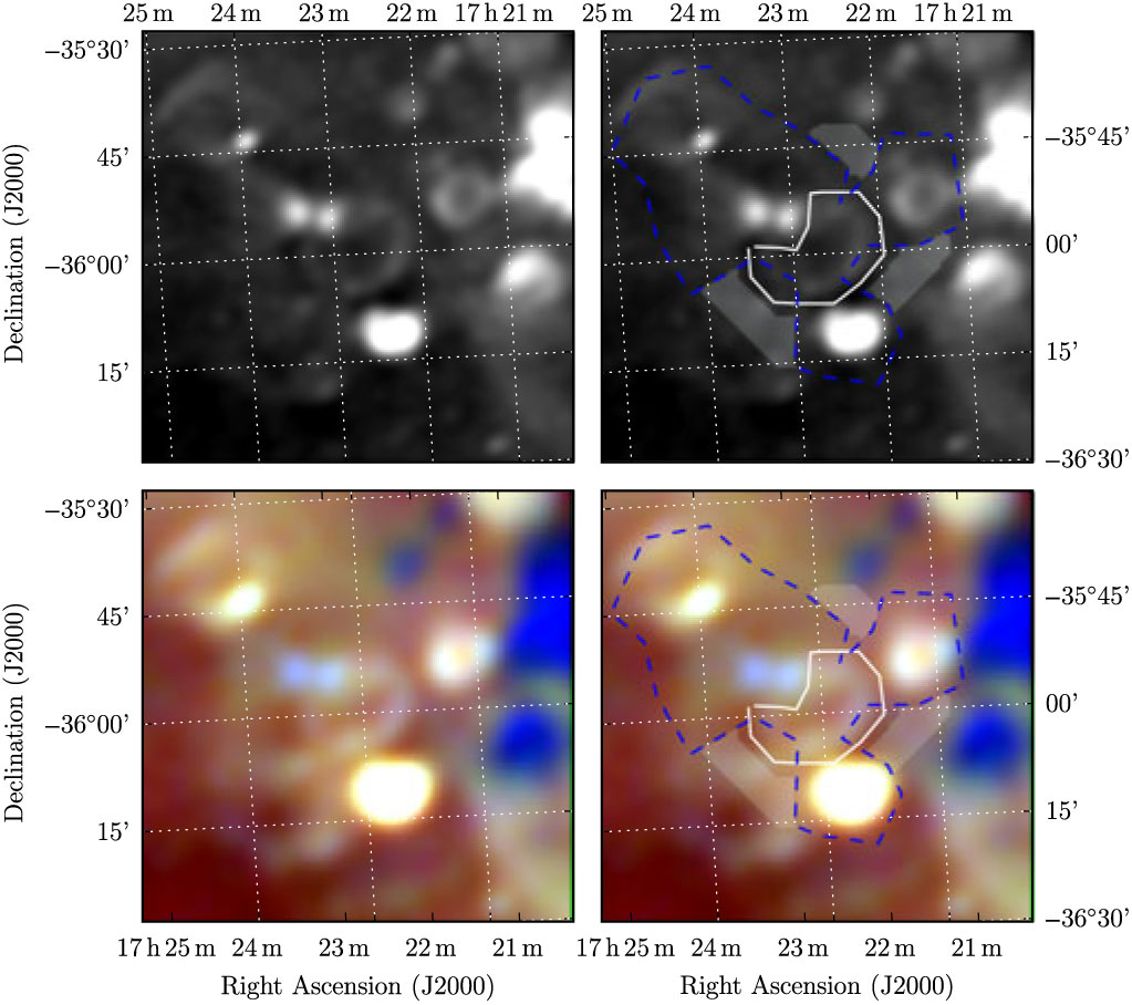
Figure B.4. Polygons drawn over GLEAM images to measure source and background flux densities for G351.4 + 0.2.
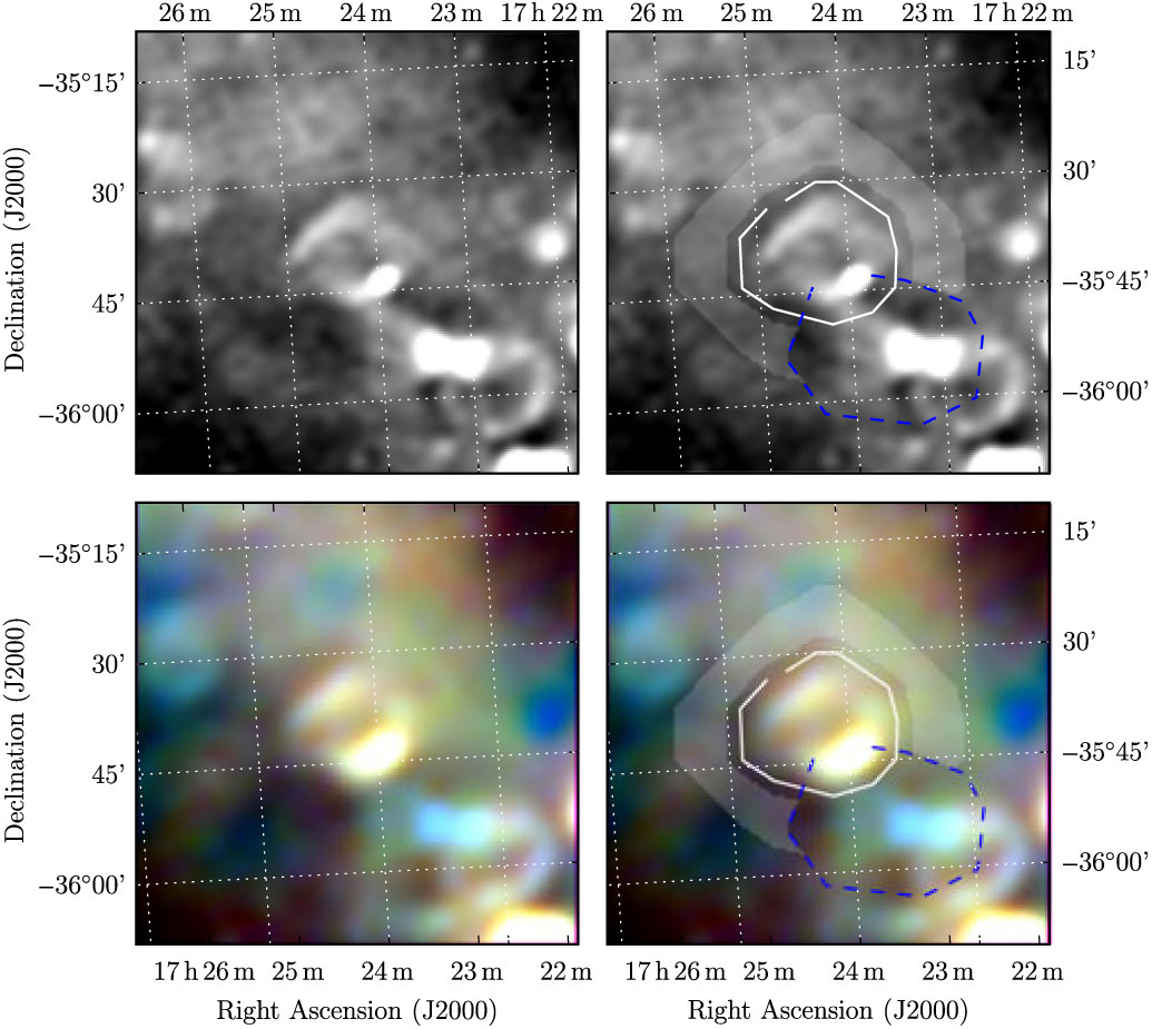
Figure B.5. Polygons drawn over GLEAM images to measure source and background flux densities for G351.9 + 0.1.
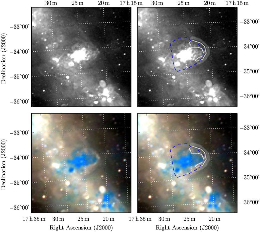
Figure B.6. Polygons drawn over GLEAM images to measure source and background flux densities for G353.0 + 0.8.
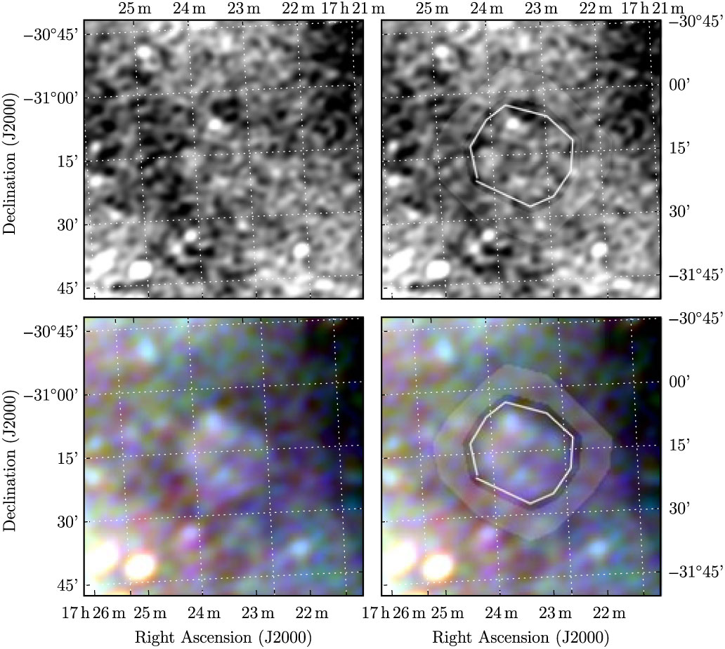
Figure B.7. Polygons drawn over GLEAM images to measure source and background flux densities for G355.4 + 2.7.
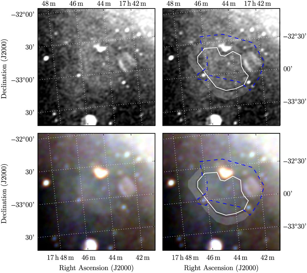
Figure B.8. Polygons drawn over GLEAM images to measure source and background flux densities for G356.5 − 1.9.
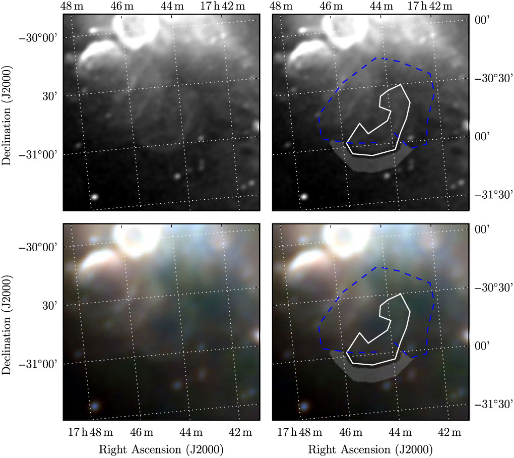
Figure B.9. Polygons drawn over GLEAM images to measure source and background flux densities for G358.3 − 0.7.
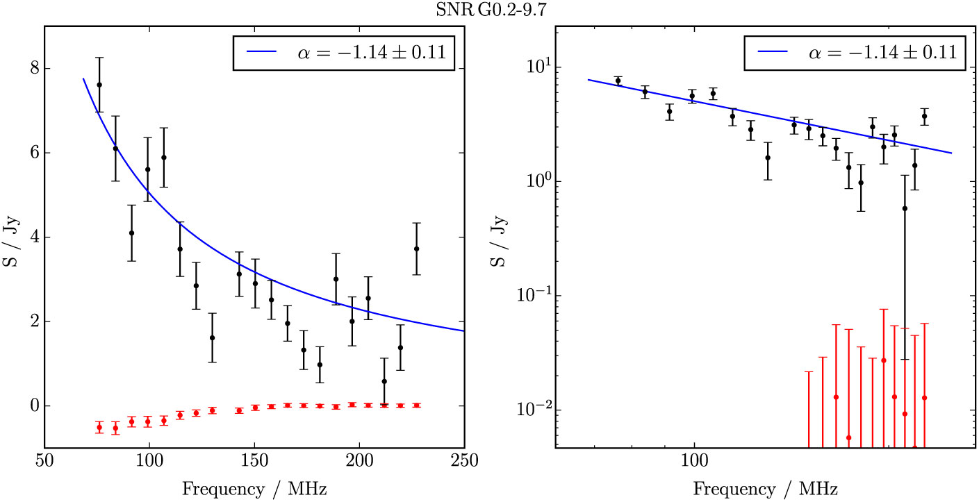
Figure B.10. Spectral fitting over the GLEAM band for G 0.1–9.7.
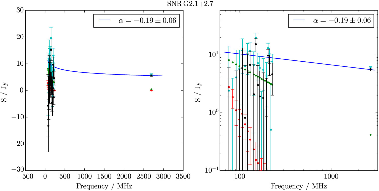
Figure B.11. Spectral fitting over the GLEAM band and Effelsberg 2.695 GHz data for G 2.1 + 2.7. Cyan points show the SNR flux densities before contaminating sources (green points) were subtracted.
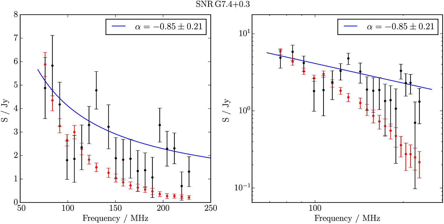
Figure B.12. Spectral fitting over the GLEAM band for G 7.4 + 0.3.
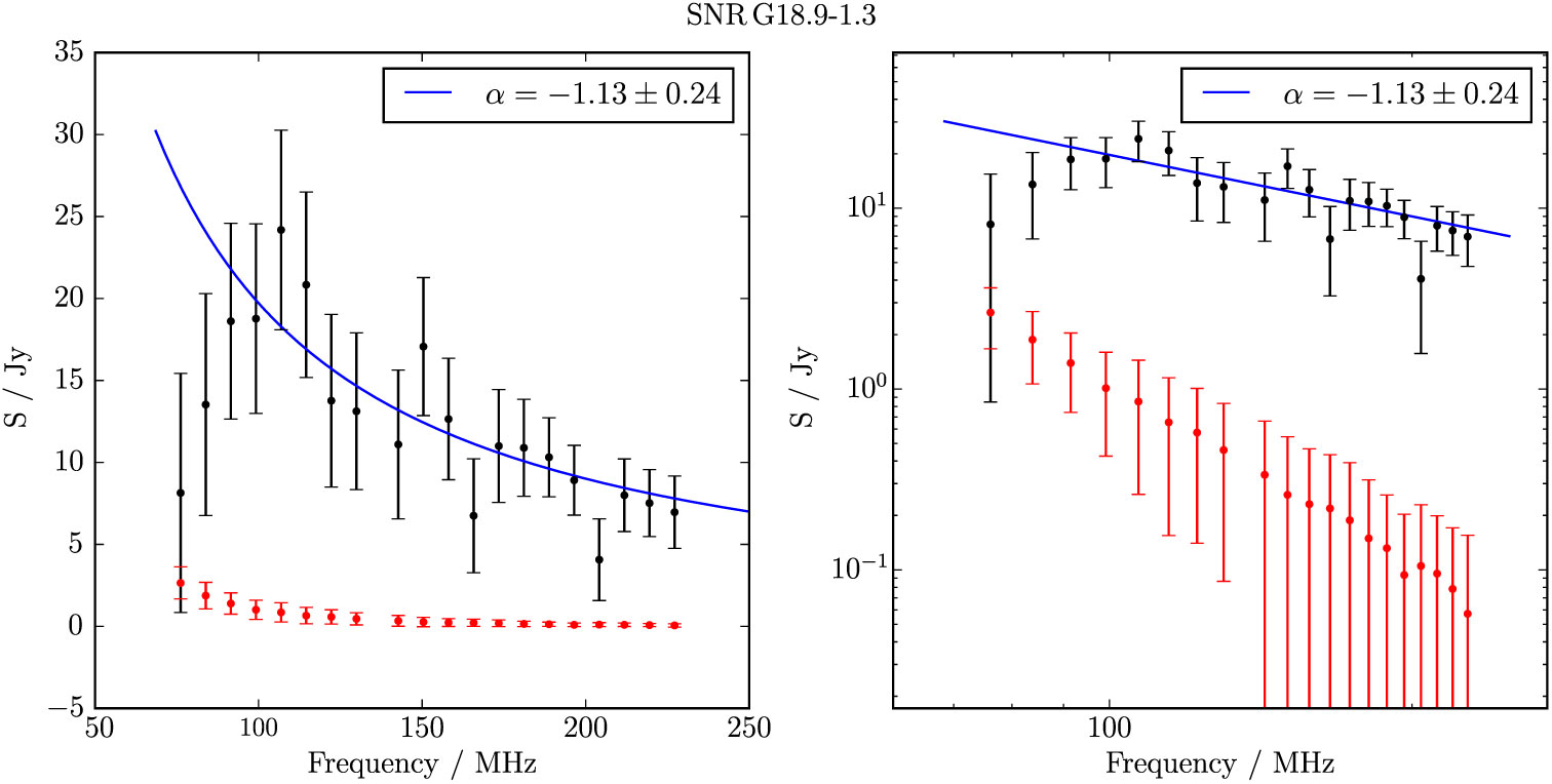
Figure B.13. Spectral fitting over the GLEAM band for G 18.9–1.2.
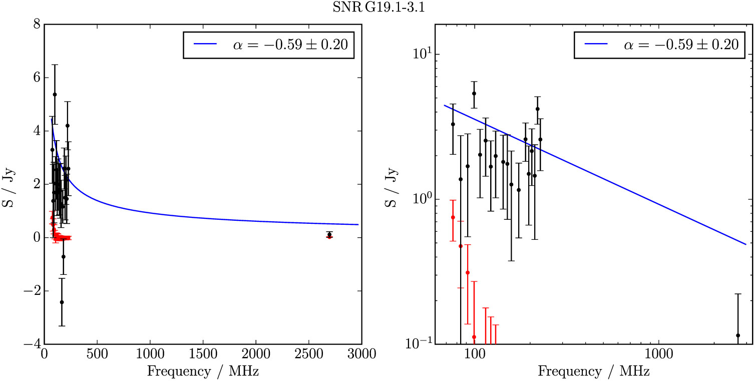
Figure B.14. Spectral fitting over the GLEAM band and Effelsberg 2.695 GHz data for G 19.1−3.1.
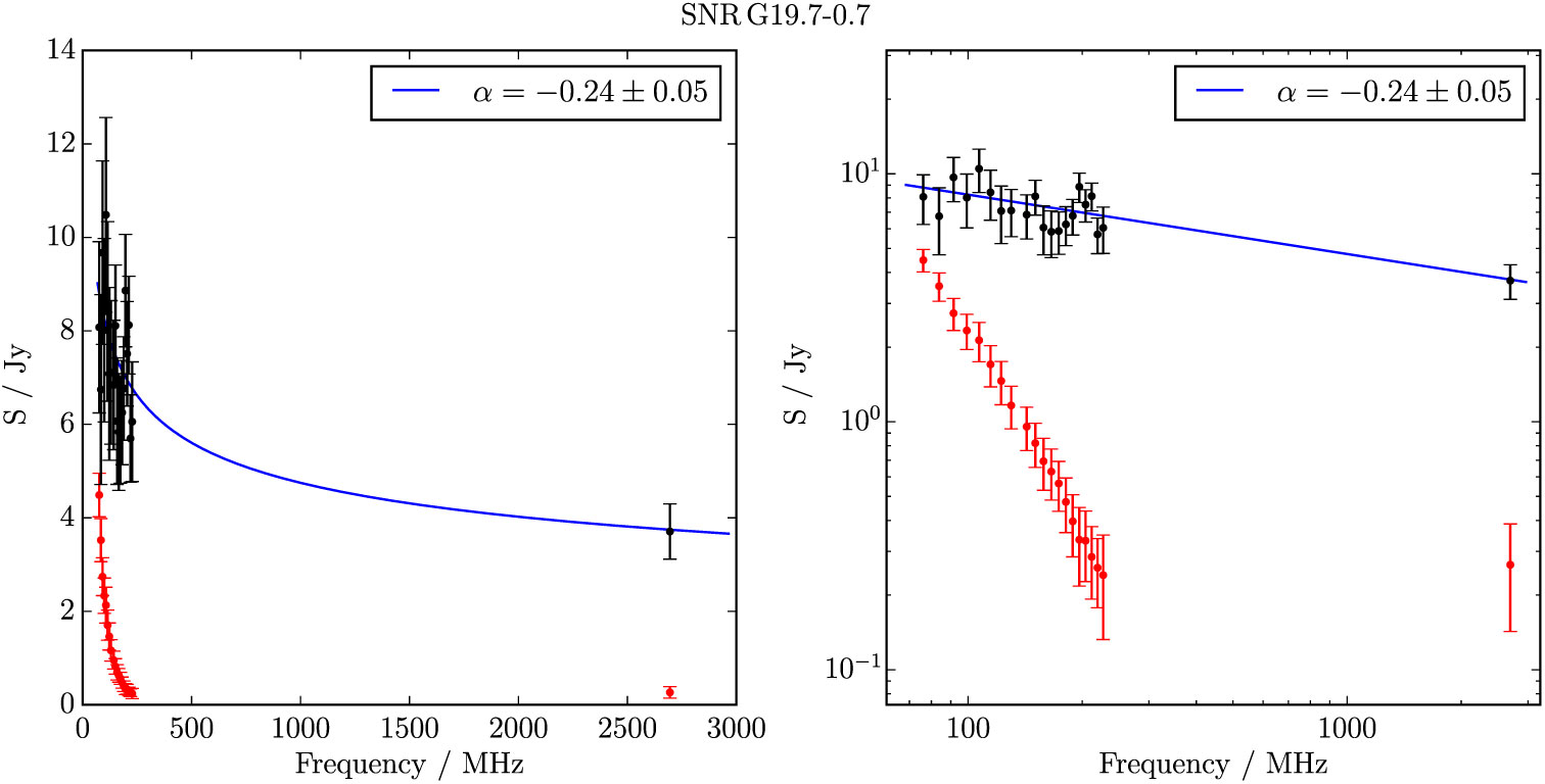
Figure B.15. Spectral fitting over the GLEAM band and Effelsberg 2.695 GHz data for G 19.7−0.7.
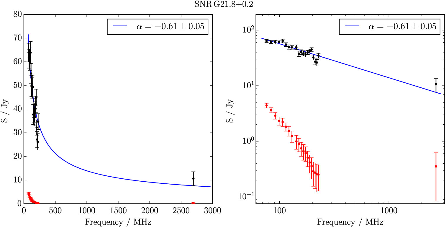
Figure B.16. Spectral fitting over the GLEAM band and Effelsberg 2.695 GHz data for G 21.8 + 0.2.
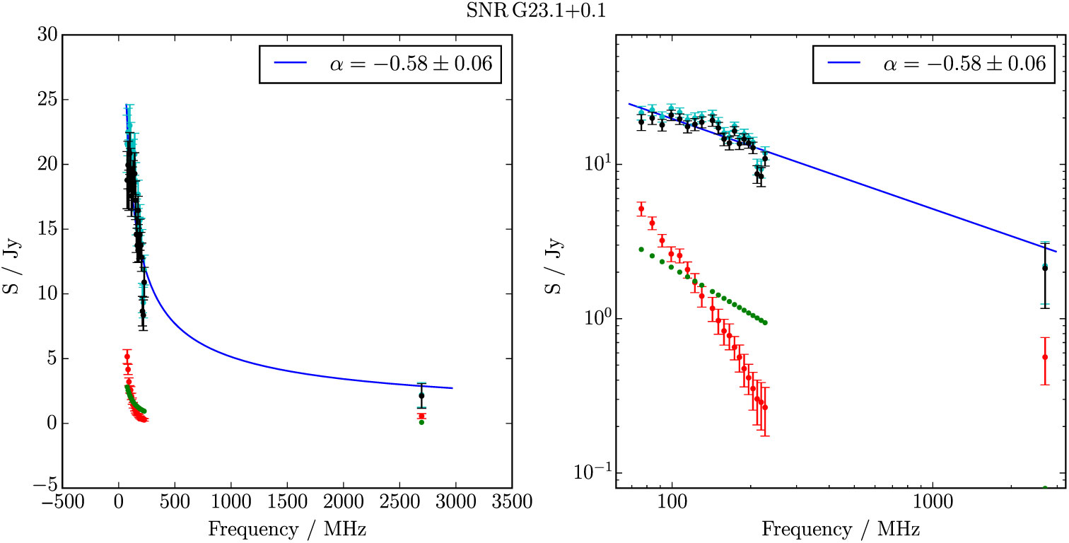
Figure B.17. Spectral fitting over the GLEAM band and Effelsberg 2.695 GHz data for G 23.1 + 0.1. Cyan points show the SNR flux densities before a contaminating source (green points) was subtracted.
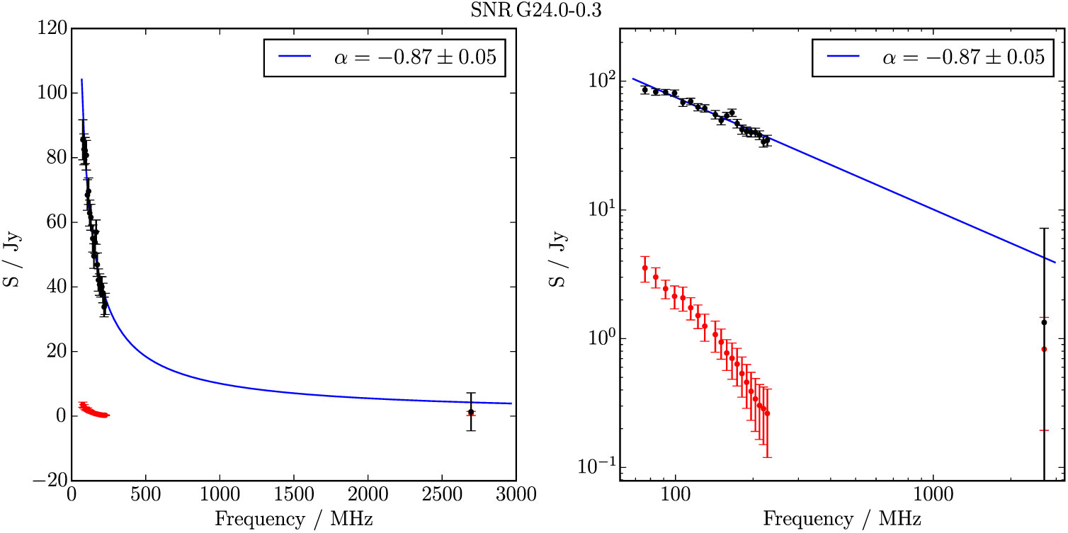
Figure B.18. Spectral fitting over the GLEAM band and Effelsberg 2.695 GHz data for G 24.0−0.3.
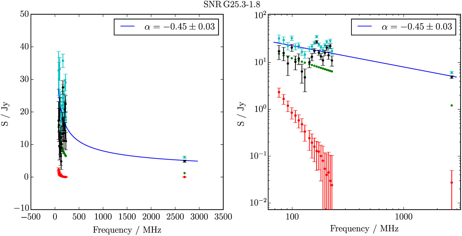
Figure B.19. Spectral fitting over the GLEAM band and Effelsberg 2.695 GHz data for G 25.3−1.8. Cyan points show the SNR flux densities before contaminating sources (green points) were subtracted.
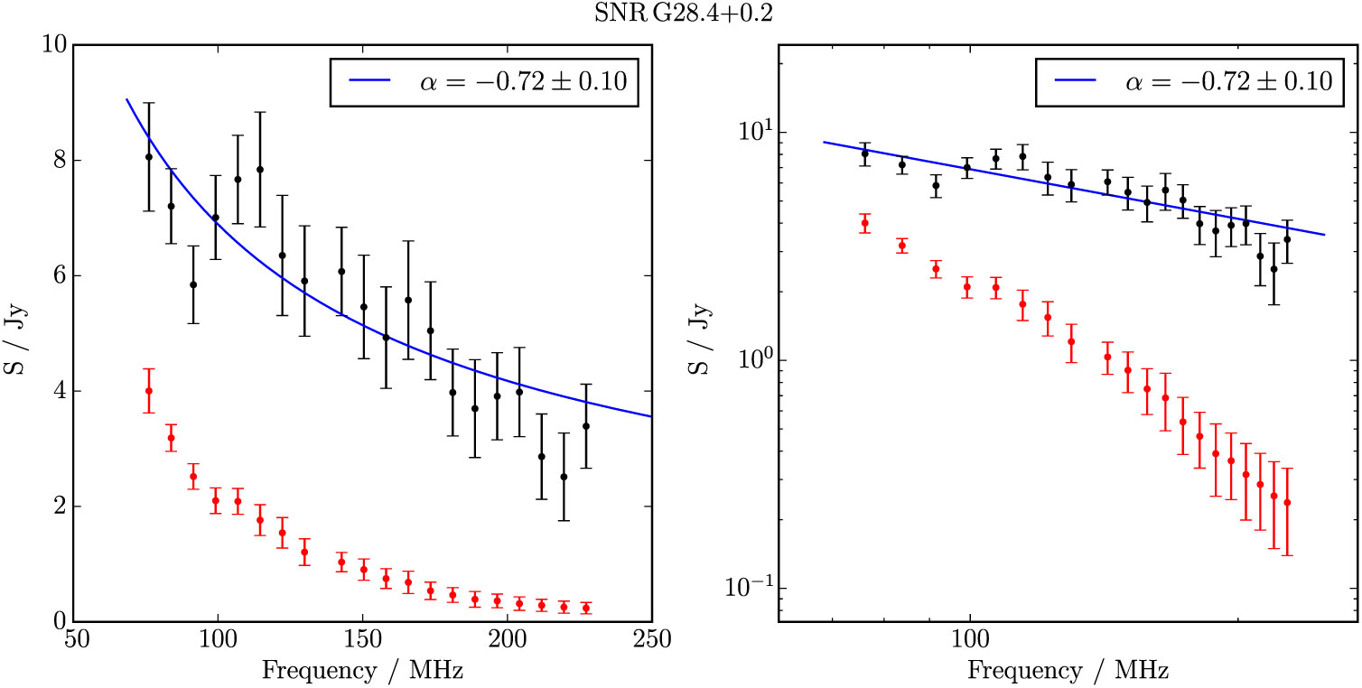
Figure B.20. Spectral fitting over the GLEAM band for G 28.3 + 0.2.
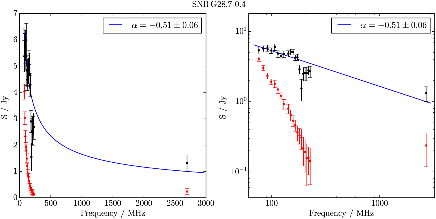
Figure B.21. Spectral fitting over the GLEAM band and Effelsberg 2.695 GHz data for G 28.7−0.4.
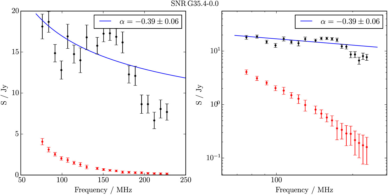
Figure B.22. Spectral fitting over the GLEAM band for G 35.3−0.0.
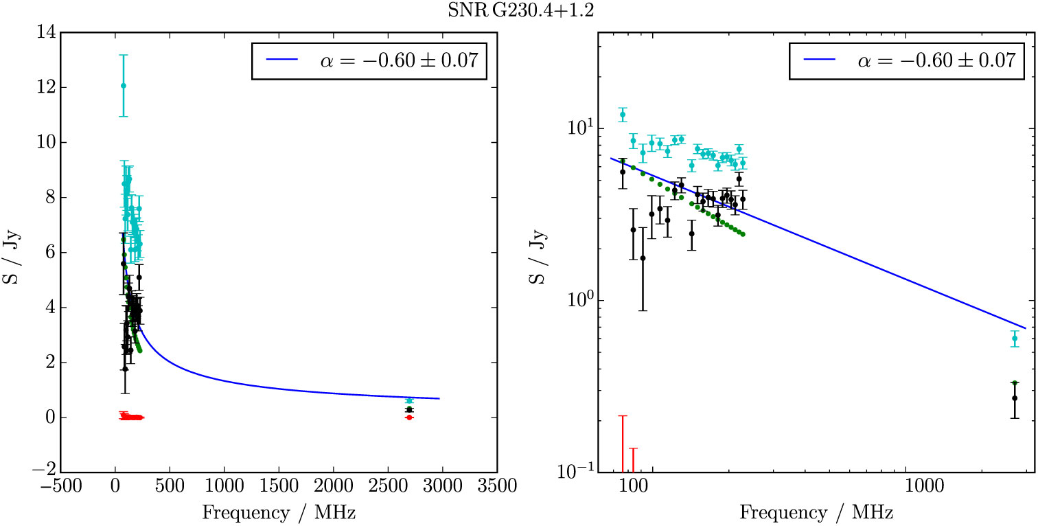
Figure B.23. Spectral fitting over the GLEAM band and Effelsberg 2.695 GHz data for G 230.4 + 1.2. Cyan points show the SNR flux densities before contaminating sources (green points) were subtracted.
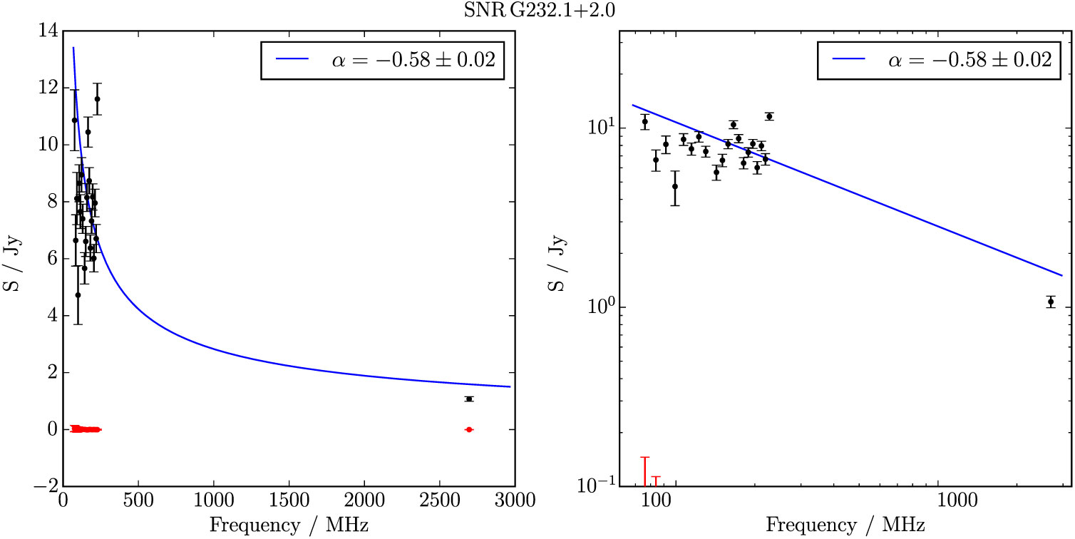
Figure B.24. Spectral fitting over the GLEAM band and Effelsberg 2.695 GHz data for G 232.1 + 2.0.
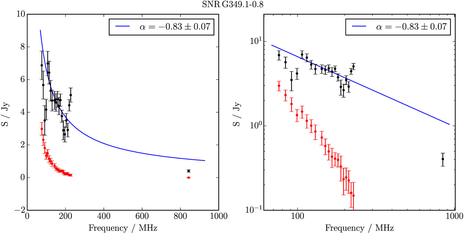
Figure B.25. Spectral fitting over the GLEAM band and MGPS 843 MHz data for G 349.1−0.8.
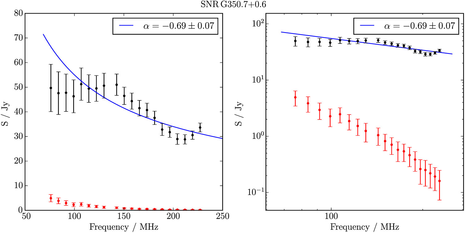
Figure B.26. Spectral fitting over the GLEAM band where ν > 150 MHz for G 350.7 + 0.6.
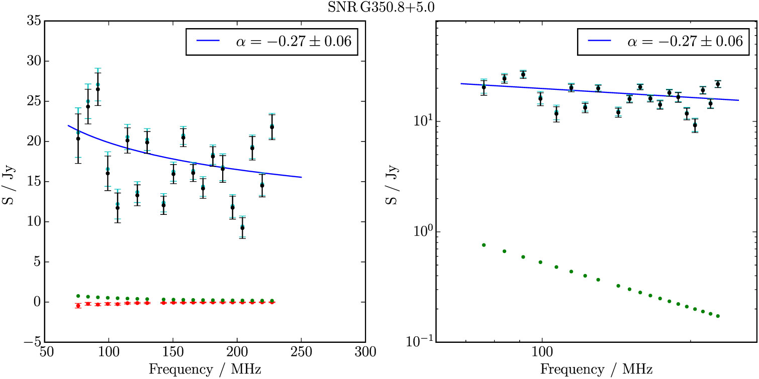
Figure B.27. Spectral fitting over the GLEAM band for G 350.8 + 5.0. Cyan points show the SNR flux densities before a contaminating source (green points) was subtracted.
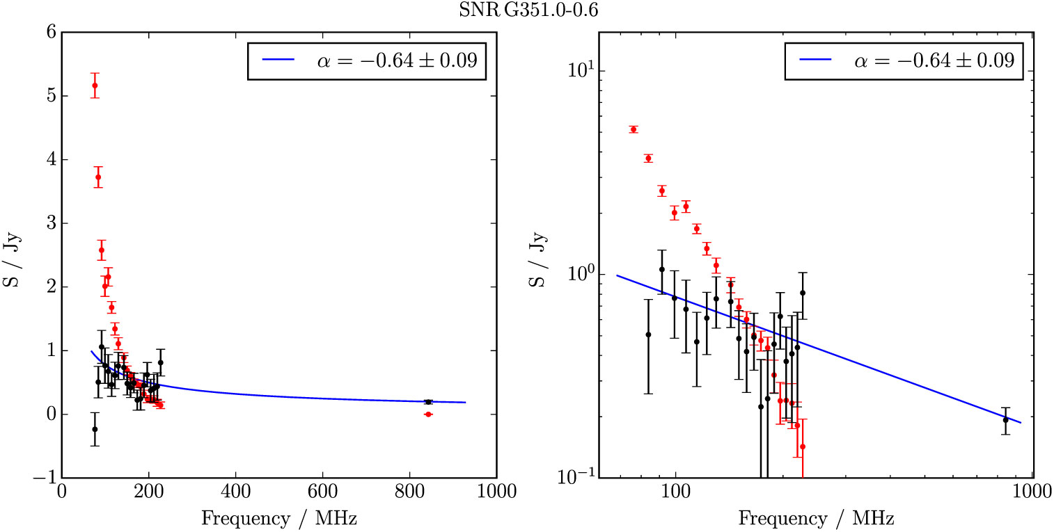
Figure B.28. Spectral fitting over the GLEAM band and MGPS 843 MHz data for G 351.0−0.6.
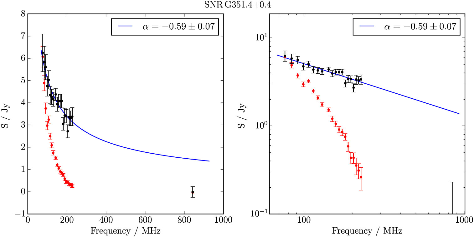
Figure B.29. Spectral fitting over the GLEAM band and MGPS 843 MHz data for G 351.4 + 0.4.
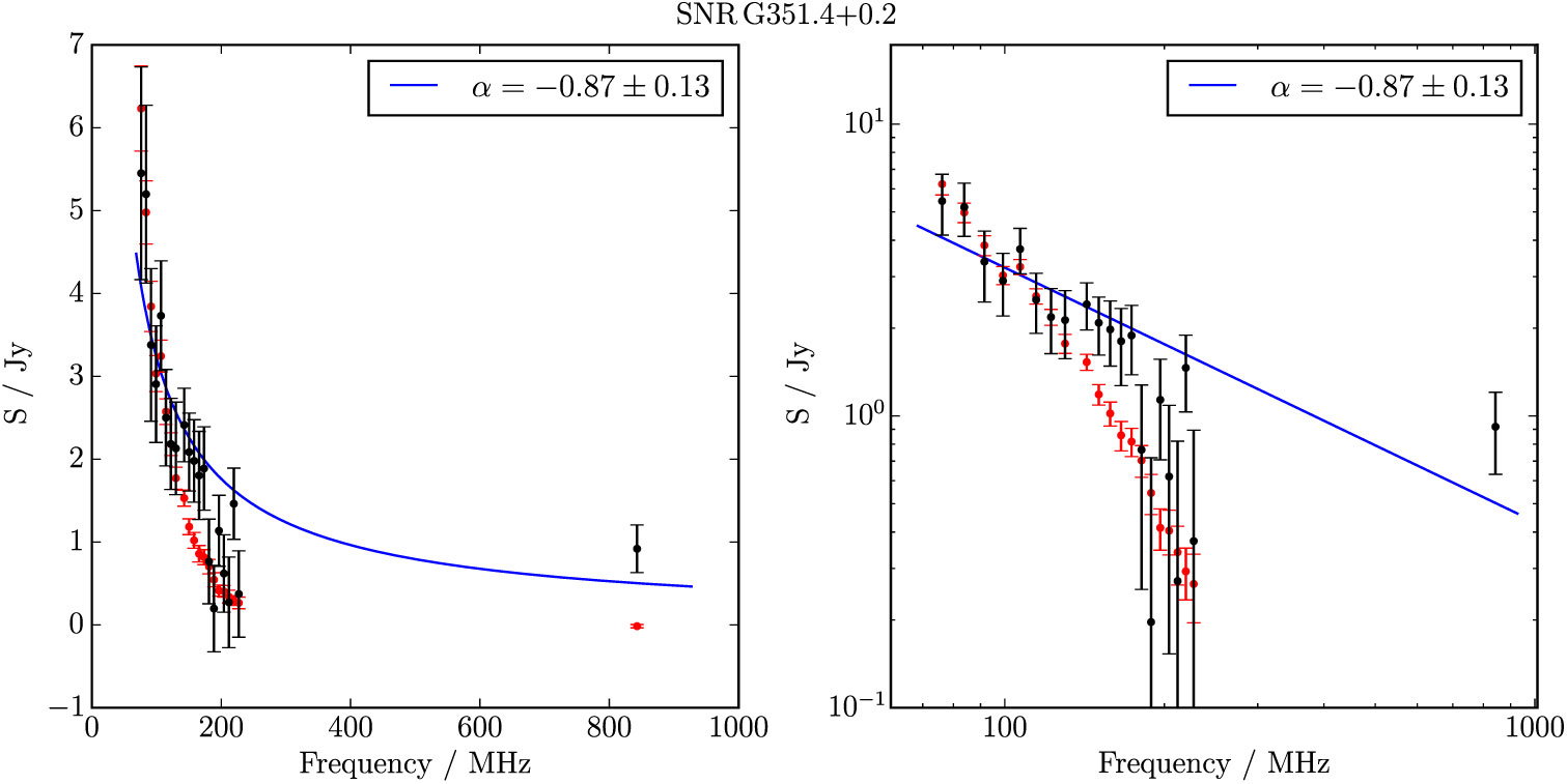
Figure B.30. Spectral fitting over the GLEAM band and MGPS 843 MHz data for G 351.4 + 0.2.
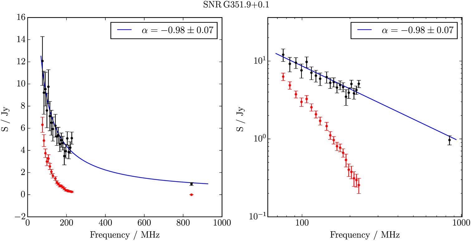
Figure B.31. Spectral fitting over the GLEAM band and MGPS 843 MHz data for G 351.9 + 0.1.
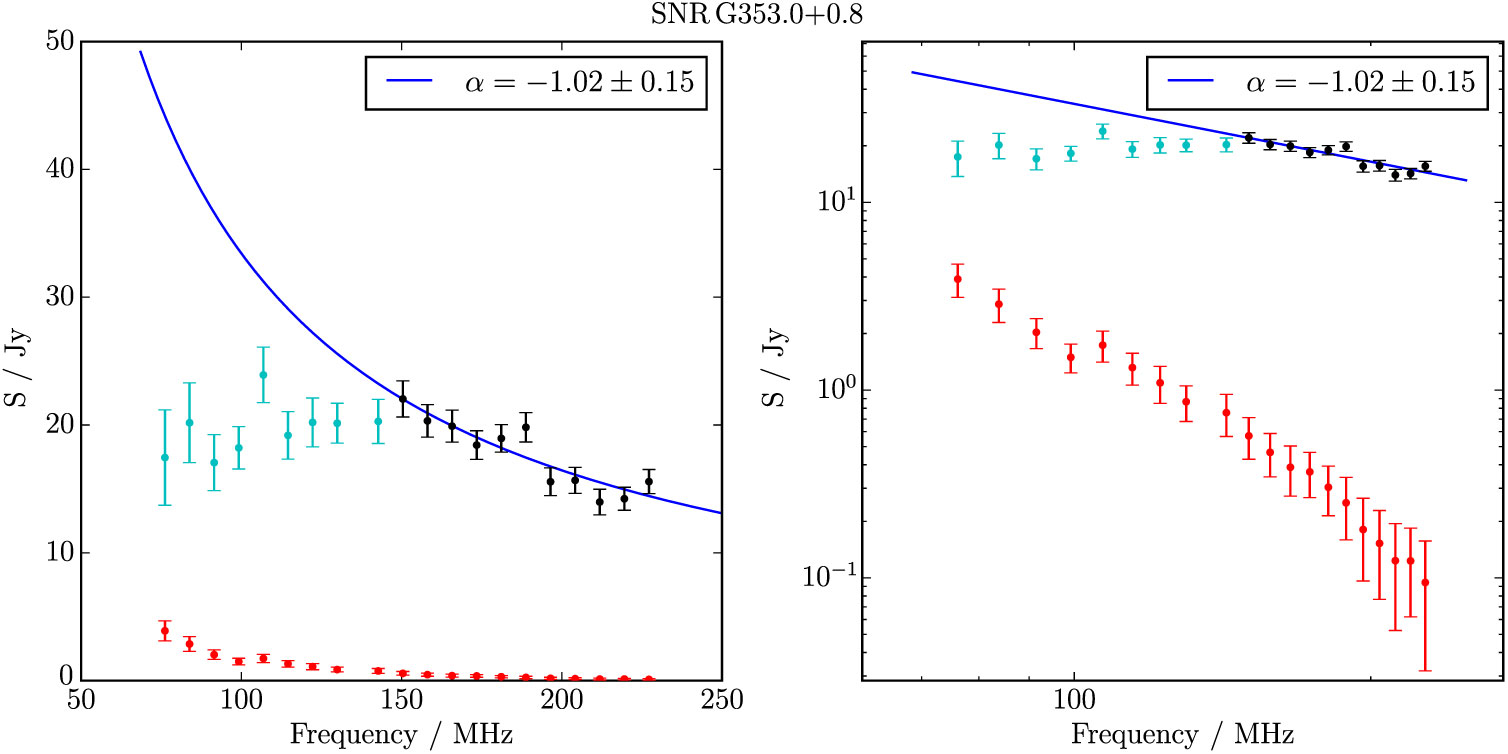
Figure B.32. Spectral fitting over the GLEAM band where ν > 150 MHz for G 353.0 + 0.8.
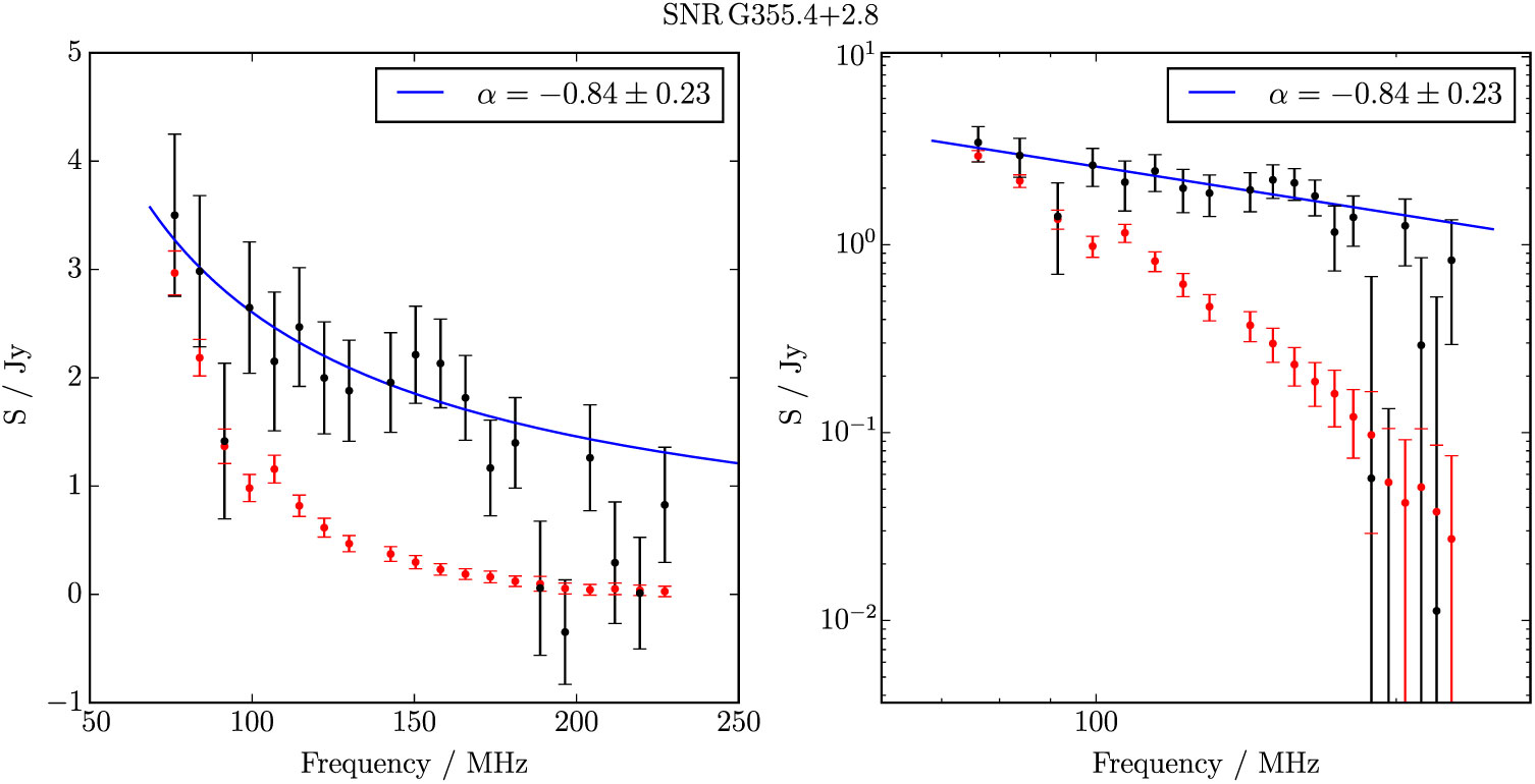
Figure B.33. Spectral fitting over the GLEAM band for G 355.4 + 2.7.
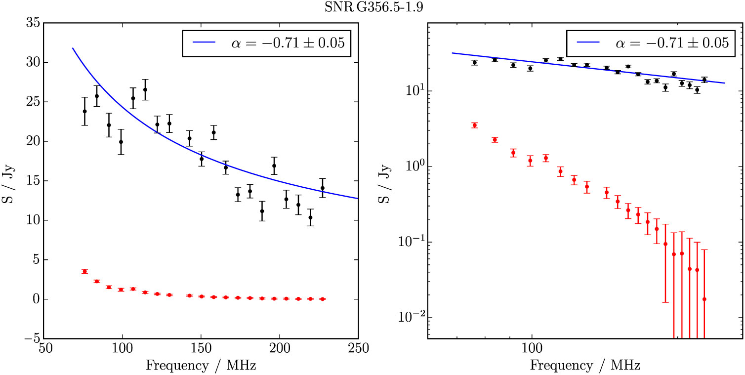
Figure B.34. Spectral fitting over the GLEAM band for G 356.5−1.9.
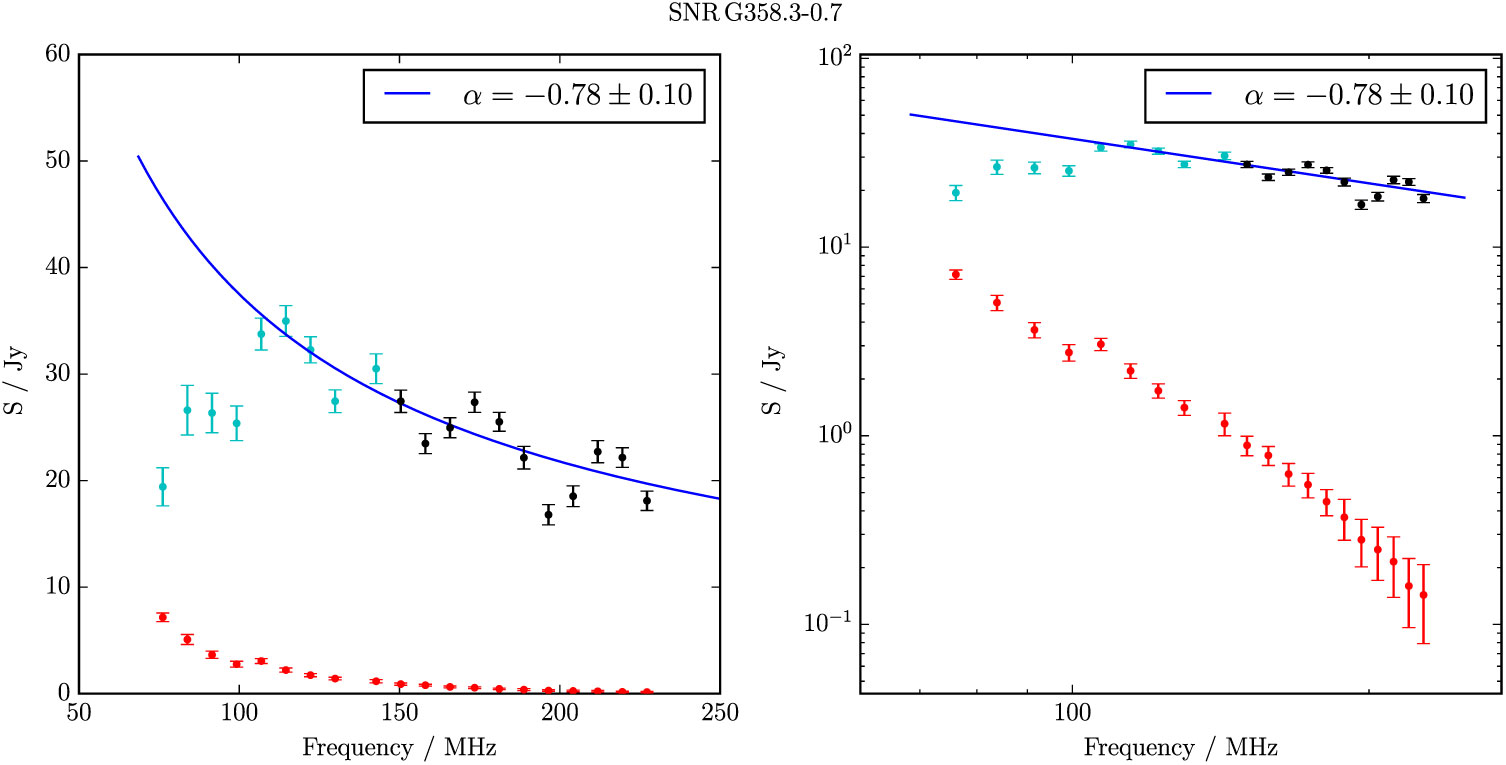
Figure B.35. Spectral fitting over the GLEAM band where ν > 150 MHz for G 358.3−0.7.