1 INTRODUCTION
Pulsar glitches are sudden increases in the rotational frequency of pulsars (predominantly observed in radio, but also seen in X-rays and gamma-rays), that are instantaneous to the accuracy of the data [with the best upper limits constraining the rise time to be less than approximately 1 min (Dodson, McCulloch, & Lewis Reference Dodson, McCulloch and Lewis2002)] and are thought to be due to the presence of a large-scale superfluid component in the neutron star. Mature neutron stars are, in fact, cold enough for neutrons to be superfluid and protons superconducting (Migdal Reference Migdal1959; Baym, Pethick, & Pines Reference Baym, Pethick and Pines1969) [see Haskell & Sedrakian (Reference Haskell and Sedrakian2017) for a recent review]. Superfluidity has a strong impact on the dynamics of the stellar interior, as a superfluid rotates by forming an array of quantised vortices which carry the circulation and mediate angular momentum exchange between the superfluid neutrons and the normal component of the star, which is tracked by the electromagnetic emission.
If vortices are strongly attracted, or ‘pinned’ to ions in the crust or flux tubes in the core of the star they cannot move out, and the superfluid cannot spin-down with the normal component, thus storing angular momentum. Sudden recoupling of the components leads to rapid angular momentum exchange and a glitch (Anderson & Itoh Reference Anderson and Itoh1975). Realistic models of pinning forces (Seveso et al. Reference Seveso, Pizzochero, Grill and Haskell2016; Wlazłowski et al. Reference Wlazłowski, Sekizawa, Magierski, Bulgac and Forbes2016) and effective masses (Chamel Reference Chamel2012, Reference Chamel2017; Watanabe & Pethick Reference Watanabe and Pethick2017) in the neutron star crusts can be used to calculate the amount of angular momentum transferred during a glitch (Pizzochero Reference Pizzochero2011; Haskell, Pizzochero, & Sidery Reference Haskell, Pizzochero and Sidery2012; Seveso, Pizzochero, & Haskell Reference Seveso, Pizzochero and Haskell2012; Andersson et al. Reference Andersson, Glampedakis, Ho and Espinoza2012; Chamel Reference Chamel2013) and compared to observations to constrain the mass of a glitching pulsar and its equation of state (Newton, Berger, & Haskell Reference Newton, Berger and Haskell2015; Ho et al. Reference Ho, Espinoza, Antonopoulou and Andersson2015; Pizzochero et al. Reference Pizzochero, Antonelli, Haskell and Seveso2017). Nevertheless, the trigger mechanism for glitches is still unknown [see Haskell & Melatos (Reference Haskell and Melatos2015) for a recent review]. The main mechanisms that have been proposed are crust quakes (Ruderman Reference Ruderman1969), hydrodynamical instabilities (Mastrano & Melatos Reference Mastrano and Melatos2005; Glampedakis & Andersson Reference Glampedakis and Andersson2009), and vortex avalanches (Cheng et al. Reference Cheng, Pines, Alpar and Shaham1988; Warszawski & Melatos Reference Warszawski and Melatos2013).
In this paper, we will focus on this last mechanism, vortex avalanches. In this model, local, fast, interactions between neighbouring vortices release stresses built up gradually over time as the star spins down. This is the hall mark of Self Organised Criticality (SOC), and in fact quantum mechanical simulations of vortices in a spinning-down trap confirm that the spin-down of the superfluid occurs via discrete vortex avalanches, and that the distribution of glitch sizes is a power-law, and the distribution of waiting times an exponential (Warszawski & Melatos Reference Warszawski and Melatos2011). This is consistent with the size and waiting time distributions of most pulsars, except for Vela and J0537-6910 (Melatos, Peralta, & Wyithe Reference Melatos, Peralta and Wyithe2008), for which an excess of large avalanches appears, with a preferred size and waiting time. Furthermore, in J0537-6910, there is a correlation between waiting times and the size of the previous glitch (Middleditch et al. Reference Middleditch, Marshall, Wang, Gotthelf and Zhang2006; Antonopoulou et al. Reference Antonopoulou, Espinoza, Kuiper and Andersson2018), which some have suggested may be due to crust quakes (Middleditch et al. Reference Middleditch, Marshall, Wang, Gotthelf and Zhang2006), but may also be the consequence of rapid driving preventing the system from self-organising, and leading to the whole pinned vorticity being expelled once the maximum of the pinning force is reached, as is the case in the ‘snowplow’ model for giant glitches (Pizzochero Reference Pizzochero2011). An excess of large avalanches may also indicate a departure of the system from SOC behaviour, and the onset of a self-organised bistable state (di Santo et al. Reference Santo, Burioni, Vezzani and Muñoz2016).
Quantum mechanical simulations, however, suffer from numerical limitations that do not allow to simulate the full neutron star system, or to model the difference in scales in a neutron star, where vortices with a coherence length ξc ≈ 10 fm are separated by a distance d v ≈ 10−3 cm. Recent work has, however, shown that even in a realistic neutron star, vortices can always move, on average, far enough to knock on neighbouring vortices without repinning, provided the relative velocity between the normal fluid and the superfluid W is close to critical velocity for unpinning, W cr, and in particular, W ≳ 0.95 W cr for standard superfluid drag parameters (Haskell & Melatos Reference Haskell and Melatos2016).
In this paper, we take a first step towards including the microphysics of vortex avalanches in larger scale hydrodynamical simulations. The situation is complex, as for a hydrodynamical treatment, one has to average over several vortices to define a coarse-grained momentum for the superfluid condensate, thus losing information on the dynamics of individual vortex unpinning and knock-on events. Large-scale hydrodynamical coupling, however, can have a strong impact on the dynamics of the system, and it is well known since the pioneering work on vortex creep of Alpar et al. (Reference Alpar, Pines, Anderson and Shaham1984a) that thermal unpinning of vortices can lead to non-linear terms in the hydrodynamical equations of motion for the superfluid velocities, and affect the post-glitch relaxation (Akbal et al. Reference Akbal, Alpar, Buchner and Pines2017).
Recently, Haskell (Reference Haskell2016) showed that random unpinning events, drawn from microphysically motivated power-law distributions, can be included in simulations. The resulting glitch distribution, however, differs from the original distribution of vortex unpinning events, and has a cut-off at small sizes, which can explain the observed deviation from a power-law of the distribution of glitches in the Crab pulsar for small sizes (Espinoza et al. Reference Espinoza, Antonopoulou, Stappers, Watts and Lyne2014). Furthermore, such an approach can also explain the different kinds of relaxation observed after glitches, also in the same star (Haskell & Antonopoulou Reference Haskell and Antonopoulou2014). Here we will follow this approach, but take a step forward in modelling the non-linear propagation of a vortex unpinning front during an avalanche.
2 SUPERFLUID HYDRODYNAMICS
We take as our starting point a hydrodynamical description of the superfluid interior of the star, in which we do not deal with the dynamics of individual vortices directly, but rather deal with averaged large-scale degrees of freedom that describe superfluid neutron velocities and densities, and those of a charge neutral fluid of protons and electrons. For the purpose of investigating the timescales associated with glitches, we will consider protons and electrons to be locked by electromagnetic interactions and flow as a single fluid (Mendell Reference Mendell1991). Following Andersson & Comer (Reference Andersson and Comer2006), we can write conservation laws for each species:
 $$\begin{equation}
\partial _t\rho _\mathrm{x}+\nabla _i(\rho _\mathrm{x}v_\mathrm{x}^i)=0,
\end{equation}$$
$$\begin{equation}
\partial _t\rho _\mathrm{x}+\nabla _i(\rho _\mathrm{x}v_\mathrm{x}^i)=0,
\end{equation}$$
where the constituent index x labels either protons (p) or neutrons (n), vi x is the velocity, and ρx is a density of respective constituent x. Note also that summation over repeated indices is implied (with the exclusion of constituent indices). The Euler equations are
 $$\begin{eqnarray}
&&(\partial _t+v_\mathrm{x}^j\nabla _j)(v_i^\mathrm{x}+\varepsilon _\mathrm{x}w_i^{\mathrm{y}\mathrm{x}})+\nabla _i(\tilde{\mu }_\mathrm{x}+\Phi )^j \nonumber \\
&&\quad +\varepsilon _\mathrm{x}w^j_{\mathrm{y}\mathrm{x}}\nabla _i v^\mathrm{x}_j=(f_i^\mathrm{x}+f_i^{\mathrm{x}\mathrm{p}})/\rho _\mathrm{x},
\end{eqnarray}$$
$$\begin{eqnarray}
&&(\partial _t+v_\mathrm{x}^j\nabla _j)(v_i^\mathrm{x}+\varepsilon _\mathrm{x}w_i^{\mathrm{y}\mathrm{x}})+\nabla _i(\tilde{\mu }_\mathrm{x}+\Phi )^j \nonumber \\
&&\quad +\varepsilon _\mathrm{x}w^j_{\mathrm{y}\mathrm{x}}\nabla _i v^\mathrm{x}_j=(f_i^\mathrm{x}+f_i^{\mathrm{x}\mathrm{p}})/\rho _\mathrm{x},
\end{eqnarray}$$
where w yxi = vi y − v xi and  $\tilde{\mu }_\mathrm{x}=\mu _\mathrm{x}/m_\mathrm{x}$ are the chemical potential per unit mass (in the following, we take m p = m n). The gravitational potential is Φ and εx is the entrainment coefficient which can account for the reduced mobility of neutrons, especially in the crust (Prix Reference Prix2004; Chamel Reference Chamel2017). The terms on the right-hand side are the contribution to the vortex-mediated mutual friction due to pinned vortices $f_i^{\text{p}\mathrm{x}}$ and to free vortices, f xi, which, for straight vortices and laminar flows, takes the form
 $$\begin{equation}
f_i^{\mathrm{x}}=\kappa n_\mathrm{v}\rho _\mathrm{n}\mathcal {B}^{^{\prime }}\epsilon _{ijk}\hat{\Omega }^i_\mathrm{n}w^k_{\mathrm{x}\mathrm{y}}+\kappa n_\mathrm{v}\rho _\mathrm{n}\mathcal {B}\epsilon _{ijk}\hat{\Omega }^j_\mathrm{n}\epsilon ^{klm}\hat{\Omega }^\mathrm{n}_l w_m^{\mathrm{x}\mathrm{y}},
\end{equation}$$
$$\begin{equation}
f_i^{\mathrm{x}}=\kappa n_\mathrm{v}\rho _\mathrm{n}\mathcal {B}^{^{\prime }}\epsilon _{ijk}\hat{\Omega }^i_\mathrm{n}w^k_{\mathrm{x}\mathrm{y}}+\kappa n_\mathrm{v}\rho _\mathrm{n}\mathcal {B}\epsilon _{ijk}\hat{\Omega }^j_\mathrm{n}\epsilon ^{klm}\hat{\Omega }^\mathrm{n}_l w_m^{\mathrm{x}\mathrm{y}},
\end{equation}$$
where Ωjn is the angular velocity of the neutrons (a hat represents a unit vector), κ = h/2m n is the quantum of circulation, n v is the vortex density per unit area, and εijk is the Levi Civita symbol. Finally, the Feynman relations link vortex density at a cylindrical radius ϖ to the rotation rate of a superfluid element:
 $$\begin{equation}
\kappa n_\mathrm{v}(\varpi )=2\tilde{\Omega }_\mathrm{n}+\varpi \frac{\partial \tilde{\Omega }_\mathrm{n}}{\partial \varpi },
\end{equation}$$
$$\begin{equation}
\kappa n_\mathrm{v}(\varpi )=2\tilde{\Omega }_\mathrm{n}+\varpi \frac{\partial \tilde{\Omega }_\mathrm{n}}{\partial \varpi },
\end{equation}$$
with
 $$\begin{equation}
\tilde{\Omega }_\mathrm{n}=\left[\Omega _\mathrm{n}+ \varepsilon _\mathrm{n}(\Omega _\mathrm{p}- \Omega _\mathrm{n})\right].
\end{equation}$$
$$\begin{equation}
\tilde{\Omega }_\mathrm{n}=\left[\Omega _\mathrm{n}+ \varepsilon _\mathrm{n}(\Omega _\mathrm{p}- \Omega _\mathrm{n})\right].
\end{equation}$$
The parameters  $\mathcal {B}$ and $\mathcal {B}^{^{\prime }}$ in the expression for the mutual friction in (3) can be expressed in terms of a dimensionless drag parameter $\mathcal {R}$, related to the standard drag parameter γd as
 $$\begin{equation}
\mathcal {R}=\frac{\gamma _{\text{d}}}{\kappa \rho _\mathrm{n}},
\end{equation}$$
$$\begin{equation}
\mathcal {R}=\frac{\gamma _{\text{d}}}{\kappa \rho _\mathrm{n}},
\end{equation}$$
and are defined as
 $$\begin{equation}
\mathcal {B}=\frac{\mathcal {R}}{1+\mathcal {R}^2}\;\;\;\;\mbox{and}\;\;\;\;\mathcal {B}^{^{\prime }}=\frac{\mathcal {R}^2}{1+\mathcal {R}^2}.
\end{equation}$$
$$\begin{equation}
\mathcal {B}=\frac{\mathcal {R}}{1+\mathcal {R}^2}\;\;\;\;\mbox{and}\;\;\;\;\mathcal {B}^{^{\prime }}=\frac{\mathcal {R}^2}{1+\mathcal {R}^2}.
\end{equation}$$
The parameter  $\mathcal {R}$ encodes the microphysics of the dissipation processes that take place in the stellar interior, and its value is highly uncertain. Nevertheless, the exact value of $\mathcal {R}$ is not crucial for the following discussion, and we will in general assume that $\mathcal {R}\ll 1$, and indicate the values we use explicitly in the examples provided.
Following Sidery, Passamonti, & Andersson (Reference Sidery, Passamonti and Andersson2010), we can simplify the problem by considering the evolution of the angular velocity of two axially symmetric rotating components. The evolution equations for the angular velocities thus take the form
 $$\begin{equation}
\dot{\Omega }_\mathrm{n}(\varpi )&=&\frac{Q(\varpi )}{\rho _\mathrm{n}}\frac{1}{1-\varepsilon _\mathrm{n}-\varepsilon _\mathrm{p}}+\frac{\varepsilon _\mathrm{n}}{(1-\varepsilon _\mathrm{n})}\dot{\Omega }_{\mbox{ext}}+F_{\text{p}}(\varpi ),
\end{equation}$$\\
$$\begin{equation}
\dot{\Omega }_\mathrm{n}(\varpi )&=&\frac{Q(\varpi )}{\rho _\mathrm{n}}\frac{1}{1-\varepsilon _\mathrm{n}-\varepsilon _\mathrm{p}}+\frac{\varepsilon _\mathrm{n}}{(1-\varepsilon _\mathrm{n})}\dot{\Omega }_{\mbox{ext}}+F_{\text{p}}(\varpi ),
\end{equation}$$\\
 $$\begin{equation}
\dot{\Omega }_\mathrm{p}(\varpi ) &=&- \frac{Q(\varpi )}{\rho _\mathrm{p}}\frac{1}{1-\varepsilon _\mathrm{n}-\varepsilon _\mathrm{p}}-\dot{\Omega }_{\mbox{ext}} -\frac{\rho _\mathrm{n}}{\rho _\mathrm{p}} F_{\text{p}}(\varpi ),
\end{equation}$$
$$\begin{equation}
\dot{\Omega }_\mathrm{p}(\varpi ) &=&- \frac{Q(\varpi )}{\rho _\mathrm{p}}\frac{1}{1-\varepsilon _\mathrm{n}-\varepsilon _\mathrm{p}}-\dot{\Omega }_{\mbox{ext}} -\frac{\rho _\mathrm{n}}{\rho _\mathrm{p}} F_{\text{p}}(\varpi ),
\end{equation}$$
 $$\begin{equation}
Q(\varpi )=\rho _\mathrm{n}\gamma \kappa n_\mathrm{v}\mathcal {B} (\Omega _\mathrm{p}-\Omega _\mathrm{n}),
\end{equation}$$
$$\begin{equation}
Q(\varpi )=\rho _\mathrm{n}\gamma \kappa n_\mathrm{v}\mathcal {B} (\Omega _\mathrm{p}-\Omega _\mathrm{n}),
\end{equation}$$
and γ = nf/n v is the fraction of vortices which are not pinned (with n f the surface density of free vortices), while  $\dot{\Omega }_{\mbox{ext}}$ is the contribution from the external spin-down torque. F p is the contribution from the pinning force. While recent progress has been made on determining the maximum value of the pinning force from microphysical calculations (Seveso et al. Reference Seveso, Pizzochero, Grill and Haskell2016; Wlazłowski et al. Reference Wlazłowski, Sekizawa, Magierski, Bulgac and Forbes2016), its exact form is not known. This does not, however, hinder our discussion, for which the exact form for F p is not necessary. It will be sufficient to assume that F p balances the contribution to the mutual friction from the (1 − γ)n v pinned vortices, below a critical threshold for the lag ΔΩC. Above ΔΩC, all vortices are free and F p = 0 [see, e.g., Seveso et al. (Reference Seveso, Pizzochero, Grill and Haskell2016) for realistic estimates of the maximum lag the pinning force can sustain]. In the following, we will thus not explicitly consider the pinning force, but simply assume a value of the critical lag ΔΩC.
We can further simplify the problem by assuming, as in Haskell et al. (Reference Haskell, Pizzochero and Sidery2012) and Haskell (Reference Haskell2016), that the proton component, consisting of the elastic crust and tightly coupled protons and electrons in the core, is rigidly rotating. This is likely to be a good approximation on timescales longer than the elastic and Alfven timescales in the crust, and simplifies our problem considerably [although see van Eysden (Reference van Eysden2014) for a discussion of the short-timescale dynamics that is neglected with this approximation]. In this approximation, the equation of motion for the protons can be obtained from (9) and is the following:
 $$\begin{equation}
\dot{\Omega }_\mathrm{p}=-\dot{\Omega }_\infty -\int \frac{\varpi ^2}{I_{\mathrm{p}}} \left[\frac{Q(\varpi )}{1-\varepsilon _\mathrm{n}-\varepsilon _\mathrm{p}}+\rho _\mathrm{n}F_{\text{p}}(\varpi )\right] {\text{d}}V,
\end{equation}$$
$$\begin{equation}
\dot{\Omega }_\mathrm{p}=-\dot{\Omega }_\infty -\int \frac{\varpi ^2}{I_{\mathrm{p}}} \left[\frac{Q(\varpi )}{1-\varepsilon _\mathrm{n}-\varepsilon _\mathrm{p}}+\rho _\mathrm{n}F_{\text{p}}(\varpi )\right] {\text{d}}V,
\end{equation}$$
where I p is the moment of inertia of the charged component.
Note that the above equations assume that vortices are straight and the rotation profile of the neutron fluid is axisymmetric. This may not be the case in the presence of strong density-dependent entrainment, as is expected in the crust (Chamel Reference Chamel2012). Antonelli & Pizzochero (Reference Antonelli and Pizzochero2017) have analysed this problem and proposed a formalism that allows one to treat the problem as axially symmetric. Given that the equations are formally equivalent, and we do not consider a density-dependent entrainment profile, we will ignore this complication in the following and continue working with the above set of equations which allow for a more transparent interpretation of the results.
It is also expected that turbulence may develop in neutron star interiors, leading to a turbulent polarised tangle of vortices and additional non-linear terms in the mutual friction force (Andersson, Sidery, & Comer Reference Andersson, Sidery and Comer2007). The importance of turbulence can be assessed by examining the evolution equation for the vorticity:
 $$\begin{eqnarray}
\frac{\partial \xi _{\mathrm{n}}^{k}}{\partial t}&=&(1-\mathcal {B}^{^{\prime }})\epsilon ^{kim}\nabla _m (\epsilon _{ijl}v_{\mathrm{n}}^{j}\xi _{\mathrm{n}}^{l})\nonumber \\
&&+\mathcal {B}{{\epsilon ^{kim}} }\nabla _m (\xi ^{\mathrm{n}}_{i}\hat{\xi }^{\mathrm{n}}_{j} v_{\mathrm{n}}^{j}-\hat{\xi }^{\mathrm{n}}_{j}\xi _{\mathrm{n}}^{j}v_{\mathrm{n}}^{i})\;,
\end{eqnarray}$$
$$\begin{eqnarray}
\frac{\partial \xi _{\mathrm{n}}^{k}}{\partial t}&=&(1-\mathcal {B}^{^{\prime }})\epsilon ^{kim}\nabla _m (\epsilon _{ijl}v_{\mathrm{n}}^{j}\xi _{\mathrm{n}}^{l})\nonumber \\
&&+\mathcal {B}{{\epsilon ^{kim}} }\nabla _m (\xi ^{\mathrm{n}}_{i}\hat{\xi }^{\mathrm{n}}_{j} v_{\mathrm{n}}^{j}-\hat{\xi }^{\mathrm{n}}_{j}\xi _{\mathrm{n}}^{j}v_{\mathrm{n}}^{i})\;,
\end{eqnarray}$$
with ξni = εijk∇jv nk, and where  $\hat{\xi }_i$ is a unit vector along ξi.
The first term on the right-hand side represents transfer of energy to small length scales, while the second leads to damping that stabilises the flow. The relative importance of two effects is determined by a parameter:
 $$\begin{equation}
q=\frac{\mathcal {B}}{1-\mathcal {B}^{^{\prime }}}.
\end{equation}$$
$$\begin{equation}
q=\frac{\mathcal {B}}{1-\mathcal {B}^{^{\prime }}}.
\end{equation}$$
It was shown by Finne et al. (Reference Finne2003) that turbulence sets in for q ⩽ 1.3. At high densities in the stellar interior  $\mathcal {B}^{\prime } \approx {\mathcal {B}}^{2} \ll 1$ so that q ≪ 1 and a superfluid neutron core is expected to be extremely susceptible to becoming turbulent, while the importance of turbulence in the crustal region is more uncertain, given the large uncertainties on $\mathcal {B}$ and $\mathcal {B}^{^{\prime }}$. To take into account the influence of turbulence and vortex curvature on the mutual friction force, one may rewrite
 $$\begin{eqnarray}
{{f}_{i}}^{mf}&=&{\rho }_{\mathrm{n}}{L}_{R}({\mathcal {B}^{^{\prime }}{\epsilon }_{ijk}{k}^{j}{{w}_{\mathrm{n}\mathrm{p}}}^{k}}+\mathcal {B}{\epsilon }_{ijk}{\epsilon }^{klm}{\hat{\kappa }}^{j}{\kappa }_{l}{w}_{m}^{\mathrm{n}\mathrm{p}}\nonumber \\
&&-\,\tilde{\nu } [\mathcal {B}^{^{\prime }}{\hat{\kappa }}^{j}{\nabla }_{j}{\kappa }_{i}+\mathcal {B}{\epsilon }_{ijk}{\kappa }^{j}{\hat{\kappa }}^{l}]{\nabla }_{l}{\hat{\kappa }}^{k})+\frac{2{L}_{T}}{3}{\rho }_{\mathrm{n}}k \mathcal {B} {{w}^{\mathrm{p}\mathrm{n}}_{i}}, \qquad
\end{eqnarray}$$
$$\begin{eqnarray}
{{f}_{i}}^{mf}&=&{\rho }_{\mathrm{n}}{L}_{R}({\mathcal {B}^{^{\prime }}{\epsilon }_{ijk}{k}^{j}{{w}_{\mathrm{n}\mathrm{p}}}^{k}}+\mathcal {B}{\epsilon }_{ijk}{\epsilon }^{klm}{\hat{\kappa }}^{j}{\kappa }_{l}{w}_{m}^{\mathrm{n}\mathrm{p}}\nonumber \\
&&-\,\tilde{\nu } [\mathcal {B}^{^{\prime }}{\hat{\kappa }}^{j}{\nabla }_{j}{\kappa }_{i}+\mathcal {B}{\epsilon }_{ijk}{\kappa }^{j}{\hat{\kappa }}^{l}]{\nabla }_{l}{\hat{\kappa }}^{k})+\frac{2{L}_{T}}{3}{\rho }_{\mathrm{n}}k \mathcal {B} {{w}^{\mathrm{p}\mathrm{n}}_{i}}, \qquad
\end{eqnarray}$$
where the last term represents polarised turbulence while the third and fourth describe the influence of an isotropic turbulent tangle. Here,
 $$\begin{equation}
\tilde{\nu }=\frac{1}{1-{\varepsilon }_{\mathrm{n}}-{\varepsilon }_{\mathrm{p}}}\nu \;,
\end{equation}$$
$$\begin{equation}
\tilde{\nu }=\frac{1}{1-{\varepsilon }_{\mathrm{n}}-{\varepsilon }_{\mathrm{p}}}\nu \;,
\end{equation}$$
with L R is the vortex length due to the rotation, such that  $\left|\nabla \times {\vec{v}}_{\mathrm{n}} \right|=2\Omega ={L}_{R}\kappa$, and L T = L − L R, with L the total length of vortex. The vector κi defines the orientation of vortex and ν is a parameter that determines the tension of the vortex [see Andersson et al. (Reference Andersson, Sidery and Comer2007) for a detailed description of the problem].
For polarised turbulence, the straight vortex term thus leads to the shortest timescales. In our work, we study the short-timescale dynamics of avalanches and ignore longer post-glitch timescale, for which additional physics regarding coupling timescales at different densities would, anyway, have to be included [see, e.g., Haskell et al. (Reference Haskell, Pizzochero and Sidery2012) and Newton et al. (Reference Newton, Berger and Haskell2015)]. Hence, turbulence is unlikely to make a qualitative difference to our results, and for computational simplicity, we ignore it in the following.
3 VORTEX PINNING AND UNPINNING
To solve the system of equations in the previous section, we still require inputs from microphysics. Apart from the fraction of neutrons, the mutual friction parameters  $\mathcal {B}$ are required. In the outer core of the neutron star, the main contribution to mutual friction is expected to come from electrons scattering on vortex cores, which leads to $\mathcal {B}\approx 10^{-4}$ (Alpar, Langer, & Sauls Reference Alpar, Langer and Sauls1984b; Andersson, Sidery, & Comer Reference Andersson, Sidery and Comer2006). In the crust, the situation is much more uncertain, as phonon scattering will lead to weak damping, with mutual friction parameters as low as $\mathcal {B}\approx 10^{-10}$, but if vortices move rapidly past pinning sites, Kelvin waves may be excited leading to $\mathcal {B}\approx 10^{-2}$ (Jones Reference Jones1990, Reference Jones1992; Epstein & Baym Reference Epstein and Baym1992). Given this level of uncertainty, and the small scales we consider, we will take $\mathcal {B}$ as a constant, free parameter, and study how our results depend on it.
In our description, however, we have also introduced an extra parameter that rescales the mutual friction coefficients, i.e., the fraction of unpinned vortices γ. This will depend specifically on the dynamics of vortices on scales smaller than the hydrodynamical scale we are discussing.
Before moving on, let us thus address the validity of our hydrodynamical description. Hydrodynamics is the natural tool to model macroscopic, observable, phenomena in neutron stars, and the key assumption is that we can track the evolution of fluid elements as they evolve. A fluid element must be small enough to be considered as a ‘point’ in the macroscopical hydrodynamical description, but also large enough to contain enough particles to allow for meaningful averaged hydrodynamical quantities and fluxes to be defined.
This is particularly relevant for a superfluid, which is irrotational and rotates by forming an array of quantised vortices which carry the circulation. In practice, this means that a coarse-grained description must average over several vortices in order to define a superfluid velocity for a fluid element, leading to a large-scale neutron fluid which is not irrotational. The minimum scale on which it is meaningful to discuss hydrodynamics is thus given by the typical inter-vortex spacing, which is of the order of
 $$\begin{equation}
d_\mathrm{v}=1\times 10^{-3} \left(\frac{P}{10 \mbox{ ms}}\right)^{1/2} \mbox{cm},
\end{equation}$$
$$\begin{equation}
d_\mathrm{v}=1\times 10^{-3} \left(\frac{P}{10 \mbox{ ms}}\right)^{1/2} \mbox{cm},
\end{equation}$$
where P is the spin period of the star. Note, however that dynamics on a smaller inter-vortex scale (on which neutrons behave as an irrotational fluid, defined by the neutron–neutron scattering length scale of approximately a micron), is crucial for determining mutual friction and pinning parameters.
Knock-on effects between vortices are likely to be fundamental for the dynamics we observe in pulsar glitches. Consider a simple model in which such effects are neglected, and one simply has random, uncorrelated, unpinning of individual vortices. In this case, the probability of unpinning n vortices during an observation time Δt, is simply a Poissonian (Warszawski & Melatos Reference Warszawski and Melatos2013):
 $$\begin{equation}
p(n)=\exp (-\theta \Delta t)\frac{(\theta \Delta t)^n}{n!}\;,
\end{equation}$$
$$\begin{equation}
p(n)=\exp (-\theta \Delta t)\frac{(\theta \Delta t)^n}{n!}\;,
\end{equation}$$
where θ is the unpinning rate for a single vortex. The result in (17) tends to a Gaussian for large Δt, suggesting that the average number of free vortices, and thus the average glitch size, should also follow a Gaussian distribution. However, this conflicts with the data in all pulsars except for PSR J0537-6910 and the Vela pulsar (Melatos et al. Reference Melatos, Peralta and Wyithe2008). The glitch size distribution in other pulsars is consistent with a power-law, with the waiting times being exponentially distributed, which is in agreement with the results obtained with small-scale quantum mechanical Gross Pitaevskii simulations of superfluid vortices in a spinning-down trap (Warszawski & Melatos Reference Warszawski and Melatos2011). It is clear that we need to understand how to scale up the dynamics observed in such simulations of ≈102 − 103 vortices, to the larger scale corse-grained hydrodynamical description where individual vortices are not resolved.
On the one side, the kind of vortex avalanches that are observed in simulations over scales of hundreds or thousands of vortices can lead to vortex depletion and accumulation on small scales and create sharp gradients in hydrodynamical simulations. On the other hand, large-scale dynamics can induce differential rotation, and significantly increase the local density of vortices, leading to knock on effects and unpinning (Warszawski, Melatos, & Berloff Reference Warszawski, Melatos and Berloff2012; Haskell & Melatos Reference Haskell and Melatos2016). For example, if vortex avalanches are free to propagate outward from high density regions at the base of the crust, towards lower density regions in which the pinning force peaks, individual vortice will encounter stronger pinning forces than in the region where they are originally unpinned. This can lead to vortices accumulating close to the maximum of the pinning force. A similar situation may occur even if vortices creep out, but the rate is not fast enough to keep up with the external driver (the electromagnetic spin-down), leading to vortex accumulation (Warszawski & Melatos Reference Warszawski and Melatos2013). This would create a vortex ‘sheet’ such as that suggested by Pizzochero (Reference Pizzochero2011), in which the vortex density is significantly higher than the steady-state density n v = 2Ωn/κ. Such a vortex sheet will gradually shift out, until the maximum lag that the pinning force can sustain is exceeded, after which all vortices are free and will rapidly move out transferring angular momentum catastrophically and giving rise to a ‘giant’ glitch, such as those observed in the Vela pulsar.
4 VORTEX SHEET
Let us now discuss this scenario in more detail and study, from a hydrodynamical point of view, how an avalanche can lead to angular momentum exchange between the superfluid and the crust.
First of all, let us define the lag between the two components:
 $$\begin{equation}
\Delta \Omega =\Omega _\mathrm{p}-\Omega _\mathrm{n}\;.
\end{equation}$$
$$\begin{equation}
\Delta \Omega =\Omega _\mathrm{p}-\Omega _\mathrm{n}\;.
\end{equation}$$
By combining equations (8) and (9), we can obtain the following evolution equation:
 $$\begin{equation}
\frac{\partial \Delta \Omega }{\partial t}=-\kappa n_\mathrm{v}\frac{\gamma \mathcal {B}}{x_\mathrm{p}(1-\varepsilon _\mathrm{n}-\varepsilon _\mathrm{p})}\Delta \Omega \;,
\end{equation}$$
$$\begin{equation}
\frac{\partial \Delta \Omega }{\partial t}=-\kappa n_\mathrm{v}\frac{\gamma \mathcal {B}}{x_\mathrm{p}(1-\varepsilon _\mathrm{n}-\varepsilon _\mathrm{p})}\Delta \Omega \;,
\end{equation}$$
where x p = ρp/ρ with ρ = ρp + ρn, and we have assumed that vortices are free (F p = 0). We ignore the external torque, as we will be studying dynamics on much shorter timescales than those on which the external spin-down is relevant.
In the standard case, one neglects differential rotation and assumes that κn v ≈ 2Ωn. Neglecting the small change in overall frequency, and taking Ωn and  $\mathcal {B}$ to be a constant, the approximate solution for the lag between the two components ΔΩ, is a damped exponential of the form (Andersson et al. Reference Andersson, Sidery and Comer2006):
 $$\begin{equation}
\Delta \Omega \approx \Delta _0 \exp {-(t/\tau )}\;,
\end{equation}$$
$$\begin{equation}
\Delta \Omega \approx \Delta _0 \exp {-(t/\tau )}\;,
\end{equation}$$
with Δ0 a constant and
 $$\begin{equation}
\tau =\frac{x_{\mathrm{p}}(1-\varepsilon _{\mathrm{n}}-\varepsilon _{\mathrm{p}})}{2\Omega _{\mathrm{n}} \gamma \mathcal {B}}\;,
\end{equation}$$
$$\begin{equation}
\tau =\frac{x_{\mathrm{p}}(1-\varepsilon _{\mathrm{n}}-\varepsilon _{\mathrm{p}})}{2\Omega _{\mathrm{n}} \gamma \mathcal {B}}\;,
\end{equation}$$
with γ taken to be constant. This is the mutual friction timescale that is usually compared to exponentially relaxing components of the spin frequency observed after glitches.
We intend to investigate a different situation here. We continue to consider the γ =constant case, and follow Cheng et al. (Reference Cheng, Pines, Alpar and Shaham1988), thus considering a vortex accumulation region in which a large number of vortices (compared to the steady-state number present in the region) has repinned, i.e., such that
 $$\begin{equation}
\kappa n_v\approx \varpi \frac{\partial }{\partial \varpi }[\Omega _\mathrm{n}+\varepsilon _\mathrm{n}(\Omega _\mathrm{p}-\Omega _\mathrm{n})]\;,
\end{equation}$$
$$\begin{equation}
\kappa n_v\approx \varpi \frac{\partial }{\partial \varpi }[\Omega _\mathrm{n}+\varepsilon _\mathrm{n}(\Omega _\mathrm{p}-\Omega _\mathrm{n})]\;,
\end{equation}$$
where the steady-state contribution κn v ≈ 2Ωn is neglected and ϖ = rsin θ is the cylindrical radius.
In this situation, it is likely that strong pinning will force vortices to repin immediately and they will not be able to adjust to the lattice-equilibrium position that would be needed for this large increase in density. By the time the approximation ϖ∂Ωn∂ϖ > 2Ωn is satisfied, one has a change in vortex density of order unity, corresponding to a similar change in vortex spacing  $l_v\approx \sqrt{n_v}$. This leads to a large change in Magnus force as vortices get closer to each other, and the vortex sheet is thus very likely to unpin (Warszawski & Melatos Reference Warszawski and Melatos2013; Haskell Reference Haskell2016).
In the presence of significant differential rotation, the equation of motion for the lag ΔΩ takes the following form:
 $$\begin{equation}
\frac{\partial \Delta \Omega (\varpi , t)}{\partial t}=\varpi \frac{\gamma \mathcal {B}(1-\varepsilon _{\mathrm{n}})}{x_\mathrm{p}(1-\varepsilon _{\mathrm{n}}-\varepsilon _{\mathrm{p}})}\Delta \Omega (\varpi ,t) \frac{\partial {\Delta \Omega (\varpi , t)}}{\partial \varpi }\;,
\end{equation}$$
$$\begin{equation}
\frac{\partial \Delta \Omega (\varpi , t)}{\partial t}=\varpi \frac{\gamma \mathcal {B}(1-\varepsilon _{\mathrm{n}})}{x_\mathrm{p}(1-\varepsilon _{\mathrm{n}}-\varepsilon _{\mathrm{p}})}\Delta \Omega (\varpi ,t) \frac{\partial {\Delta \Omega (\varpi , t)}}{\partial \varpi }\;,
\end{equation}$$
where we have assumed that, at least locally, the proton fluid (possibly the crust in this case) is rigidly rotating so that ∂ϖΩp = 0 and thus ∂ϖΔΩ = −∂ϖΩn. If we make the further approximation that in the crust the amount by which the vortices move is small compared to ϖs ≈ 106 cm, and thus consider ϖ = ϖs constant, the equation above becomes
 $$\begin{equation}
\frac{\partial \Delta \Omega (\varpi , t)}{\partial t}=-\beta \Delta \Omega (\varpi ,t) \frac{\partial {\Delta \Omega (\varpi , t)}}{\partial \varpi } \;,
\end{equation}$$
$$\begin{equation}
\frac{\partial \Delta \Omega (\varpi , t)}{\partial t}=-\beta \Delta \Omega (\varpi ,t) \frac{\partial {\Delta \Omega (\varpi , t)}}{\partial \varpi } \;,
\end{equation}$$
with
 $$\begin{equation}
\beta =\varpi _s \frac{\gamma \mathcal {B}}{x_\mathrm{p}(1-\varepsilon _{\mathrm{n}}-\varepsilon _{\mathrm{p}})}(\varepsilon _{\mathrm{n}}-1).
\end{equation}$$
$$\begin{equation}
\beta =\varpi _s \frac{\gamma \mathcal {B}}{x_\mathrm{p}(1-\varepsilon _{\mathrm{n}}-\varepsilon _{\mathrm{p}})}(\varepsilon _{\mathrm{n}}-1).
\end{equation}$$
Finally, with the substitution Δ* = βΔΩ, we obtain as a general form of equation
 $$\begin{equation}
\frac{\partial \Delta ^*(\varpi , t)}{\partial t}=-\Delta ^*(\varpi ,t) \frac{\partial {\Delta ^*(\varpi , t)}}{\partial \varpi } .
\end{equation}$$
$$\begin{equation}
\frac{\partial \Delta ^*(\varpi , t)}{\partial t}=-\Delta ^*(\varpi ,t) \frac{\partial {\Delta ^*(\varpi , t)}}{\partial \varpi } .
\end{equation}$$
This is a Burgers equation, and allows travelling waves as solutions. In particular, let us consider the following initial conditions, corresponding to a large number of vortices accumulated close to the maximum of the pinning force, such that the lag is negligible prior to the vortex accumulation region, and approximately the maximum value ΔΩM after an infinitesimally thin accumulation region located at ϖ0:
 $$\begin{equation}
\Delta \Omega (t=0)=\Delta \Omega _M \Theta ( \varpi -\varpi _0)\;,
\end{equation}$$
$$\begin{equation}
\Delta \Omega (t=0)=\Delta \Omega _M \Theta ( \varpi -\varpi _0)\;,
\end{equation}$$
corresponding to (given that we take β to be a constant)
 $$\begin{equation}
\Delta ^{*} (t=0)=\Delta ^{*}_M \Theta ( \varpi -\varpi _0)\;,
\end{equation}$$
$$\begin{equation}
\Delta ^{*} (t=0)=\Delta ^{*}_M \Theta ( \varpi -\varpi _0)\;,
\end{equation}$$
where Θ(x) is the Heaviside step function. A solution to this equation which conserves the total number of vortices (in the approximation ϖs = constant) is a fan wave:
 $$\begin{equation}
\Delta ^{*}(t,\varpi )&=&\frac{\varpi -\varpi _0}{t}\;\;\;\mbox{for}\;\;\;\varpi <\varpi _F,
\end{equation}$$\\
$$\begin{equation}
\Delta ^{*}(t,\varpi )&=&\frac{\varpi -\varpi _0}{t}\;\;\;\mbox{for}\;\;\;\varpi <\varpi _F,
\end{equation}$$\\
 $$\begin{equation}
\Delta ^{*}(t,\varpi )&=&\Delta ^{*}_M\;\;\;\;\mbox{for}\;\;\;\varpi \ge \varpi _F \;,
\end{equation}$$
$$\begin{equation}
\Delta ^{*}(t,\varpi )&=&\Delta ^{*}_M\;\;\;\;\mbox{for}\;\;\;\varpi \ge \varpi _F \;,
\end{equation}$$
 $$\begin{equation}
\Delta \Omega (t,\varpi )&=&\frac{\varpi -\varpi _0}{\beta t}\;\;\;\mbox{for}\;\;\;\varpi <\varpi _F,
\end{equation}$$\\
$$\begin{equation}
\Delta \Omega (t,\varpi )&=&\frac{\varpi -\varpi _0}{\beta t}\;\;\;\mbox{for}\;\;\;\varpi <\varpi _F,
\end{equation}$$\\
 $$\begin{equation}
\Delta \Omega (t,\varpi )&=&\Delta \Omega _M\;\;\;\;\mbox{for}\;\;\;\varpi \ge \varpi _F \;,
\end{equation}$$
$$\begin{equation}
\Delta \Omega (t,\varpi )&=&\Delta \Omega _M\;\;\;\;\mbox{for}\;\;\;\varpi \ge \varpi _F \;,
\end{equation}$$ $v_F=\beta \Delta \Omega _M=-\Delta \Omega _M\varpi _s \frac{\gamma \mathcal {B}}{x_\mathrm{p}(1-\varepsilon _{\mathrm{n}}-\varepsilon _{\mathrm{p}})}(1-\varepsilon _{\mathrm{n}})$ (keeping in mind that in a pulsar the lag ΔΩ is negative). After the wave has travelled a distance d ≈ 102 cm, our approximation ( $\varpi \frac{\partial }{\partial \varpi }\left[\Omega _\mathrm{n}+\varepsilon _\mathrm{n}(\Omega _\mathrm{p}-\Omega _\mathrm{n})\right]>2\Omega _\mathrm{n}$) breaks down and one has once again κn v ≈ 2Ω. Furthermore, as the lag is below the critical value, one can expect repinning. However, the above analysis shows vortex accumulation can lead to rapid outward motion of vortices, on length scales much larger that the inter vortex motion, that may drive further avalanches as it travels through the medium.
The number of vortices in the front is (assuming ϖ constant)
 $$\begin{eqnarray}
N_\mathrm{v}&=&\int \frac{n_\mathrm{v}}{\kappa } {\text{d}}S \approx 2\pi \int \frac{\varpi _s^2}{\kappa }\frac{\partial \Delta \Omega }{\partial \varpi } {\text{d}}r \nonumber \\
&=& \frac{\varpi _s^2}{\kappa } \Delta \Omega \bigg |^{\varpi _F}_{\varpi _0}\approx \frac{\Delta \Omega _M}{\kappa }\;,
\end{eqnarray}$$
$$\begin{eqnarray}
N_\mathrm{v}&=&\int \frac{n_\mathrm{v}}{\kappa } {\text{d}}S \approx 2\pi \int \frac{\varpi _s^2}{\kappa }\frac{\partial \Delta \Omega }{\partial \varpi } {\text{d}}r \nonumber \\
&=& \frac{\varpi _s^2}{\kappa } \Delta \Omega \bigg |^{\varpi _F}_{\varpi _0}\approx \frac{\Delta \Omega _M}{\kappa }\;,
\end{eqnarray}$$
which is conserved by the solution.
Let us now consider the region upstream from the vortex accumulation region. Here, there must be a depletion region in which the lag has to change from its equilibrium value ΔΩe to 0 over a short lengthscale. This can be determined by imposing that vortex density vanish, i.e.
 $$\begin{equation}
\kappa n_\mathrm{v}= 2\Omega _\mathrm{n}+\varpi \frac{\partial \Omega _\mathrm{n}}{\partial \varpi } = 0\;,
\end{equation}$$
$$\begin{equation}
\kappa n_\mathrm{v}= 2\Omega _\mathrm{n}+\varpi \frac{\partial \Omega _\mathrm{n}}{\partial \varpi } = 0\;,
\end{equation}$$
which gives, close to a point ϖd
 $$\begin{equation}
\Omega _\mathrm{n}=\Omega _0\left(\frac{\varpi _d}{\varpi }\right)^2.
\end{equation}$$
$$\begin{equation}
\Omega _\mathrm{n}=\Omega _0\left(\frac{\varpi _d}{\varpi }\right)^2.
\end{equation}$$
Expanding around ϖd in δr = (ϖ − ϖ0), we see that the lag decreases as
 $$\begin{equation}
\Delta \Omega =\Delta \Omega _0-2\Omega _0\frac{\delta r}{\varpi _0}.
\end{equation}$$
$$\begin{equation}
\Delta \Omega =\Delta \Omega _0-2\Omega _0\frac{\delta r}{\varpi _0}.
\end{equation}$$
For typical parameters, this gives a decrease in lag over a lengthscale δr ≈ 10–100 cm, which is the same lengthscale over which our approximation is valid.
Nevertheless, to continue our initial analysis, we will make the simplifying assumption that in this region the drop in lag can be approximated as a steep drop of the form
 $$\begin{equation}
\Delta \Omega =\Delta \Omega _M\Theta (\varpi _{d}-\varpi )\;,
\end{equation}$$
$$\begin{equation}
\Delta \Omega =\Delta \Omega _M\Theta (\varpi _{d}-\varpi )\;,
\end{equation}$$
but one should keep in mind that this is at the limit of validity for using equation (24), given the estimate in (36) In this case, as vortex unpinning causes a perturbation in Magnus force due to the lack of vortices in their equilibrium positions, there will be a backward propagating unpinning avalanche. The solution corresponds to a forward moving shock that describes vortices moving out to fill the void, of the form
 $$\begin{equation}
\Delta \Omega =\Delta \Omega _M\Theta (\varpi _{d}-\varpi )\;,
\end{equation}$$
$$\begin{equation}
\Delta \Omega =\Delta \Omega _M\Theta (\varpi _{d}-\varpi )\;,
\end{equation}$$
where the position of the shock is determined by ϖd = v St, with v S = βΔΩM/2.
5 UNPINNING VORTEX WAVES
In the previous section, we showed how, by solving analytically equation (19), we can describe an unpinning wave that travels as a shock in the fluid. In doing so, however, we have had to make the assumption that γ, the fraction of unpinned vortices, is a constant, and neglect the steady-state contribution to the vortex number density κn v ≈ 2Ωn. In practice, this allows us to only evolve the equations of motion as long as ϖ∂ϖΩn ≪ 2Ω.
To go beyond this approximation, we have to provide an evolution equation for the unpinned fraction γ. This is a complex problem, given that the microphysics that governs vortex pinning acts on scales much smaller than the hydrodynamical scale. Attempts have been made in this direction in the context of superfluid turbulence, in which case an additional equation is included to model the evolution of the vortex length (Mongiovì, Russo, & Sciacca Reference Mongiovì, Russo and Sciacca2017). Here, however, we will not derive a full mean-field description of vortex unpinning, but rather focus on how different prescriptions for short-timescale movement of vortices during an avalanche can affect astrophysical observables. Another approach to constructing global models was taken in Fulgenzi, Melatos, & Hughes (Reference Fulgenzi, Melatos and Hughes2017), where the angular velocity lag between the pulsars’s superfluid interior and a rigid crust is considered as fluctuating according to a state-dependent Poisson process. In this case, local vortex motion and knock-on effects are not taken into account in the hydrodynamics.
In analogy with mean-field approaches to the study of sand piles and of self-organised critical systems more generally, we can assume that one has a time evolution equation for γ, with local terms which depend only on powers of γ itself, that govern the long-scale relaxation of the system close to equilibrium, due to random unpinning and repinning. The evolution equations for γ thus take the form
 $$\begin{equation}
\frac{\partial \gamma }{\partial t}=\sum _n \alpha _n \gamma ^n+\xi f(\gamma , \partial _r\gamma )\;,
\end{equation}$$
$$\begin{equation}
\frac{\partial \gamma }{\partial t}=\sum _n \alpha _n \gamma ^n+\xi f(\gamma , \partial _r\gamma )\;,
\end{equation}$$
where αn and ξ are coefficients, and f(γ, ∂rγ) is a function of γ and its spatial derivatives that models transport of vortices. In standard SOC models, f would simply be a diffusion term of the form f = ∇2γ. In our case, the Magnus force sets a preferred direction for vortex motion, so we will consider different forms of advection terms rather than diffusion. The terms ∑nαnγn model the competition between unpinning and repinning on the microscopic level, and set the steady-state equilibrium of the system. The addition of noise to (39) can then lead to departures from equilibrium and avalanches. This is, however, a complex problem, well beyond the scope of the current analysis. Here, we intend to take a first step towards the analysis of the propagation of avalanches; therefore, we will neglect the terms ∑nαnγn, that set the background equilibrium on timescales longer that those of an avalanche and simply analyse how a large perturbation propagates by considering an evolution equation of the form:
 $$\begin{equation}
\frac{\partial \gamma }{\partial t}=\xi f(\gamma , \partial _r\gamma ).
\end{equation}$$
$$\begin{equation}
\frac{\partial \gamma }{\partial t}=\xi f(\gamma , \partial _r\gamma ).
\end{equation}$$
5.1. Vortex advection
Let us consider different setups to describe the evolution of the unpinned fraction γ, neglecting the entrainment for simplicity. Given the phenomenological nature of this investigation, we consider three setups.
In the first setup, we consider a non-linear problem with non-constant coefficient in the advection term so that we allow vortices to advect with the velocity that is equal to the velocity of the shock wave. This is done to synchronise the repining process and angular momentum exchange, and account for vortex unpinning in the front. We explicitly take into account the steady-state contribution κn v ≈ 2Ωn in equation (22), but assume that all vortices are unpinned in the front (γ = 1) in order to decouple the advection term in the lag from the equations of motion for γ. Our first setup (case I) thus takes the following form for ΔΩ:
 $$\begin{equation}
\frac{\partial \Delta \Omega }{\partial t} = \frac{B}{{x}_{\mathrm{p}}}{\varpi }_{s} \Delta \Omega \frac{\partial \Delta \Omega }{\partial \omega }-2\Omega \Delta \Omega \frac{\gamma \mathcal {B} }{{x}_{\mathrm{p}}} \;,
\end{equation}$$
$$\begin{equation}
\frac{\partial \Delta \Omega }{\partial t} = \frac{B}{{x}_{\mathrm{p}}}{\varpi }_{s} \Delta \Omega \frac{\partial \Delta \Omega }{\partial \omega }-2\Omega \Delta \Omega \frac{\gamma \mathcal {B} }{{x}_{\mathrm{p}}} \;,
\end{equation}$$
and the equation for γ is
 $$\begin{equation}
\frac{\partial \gamma }{\partial t} = \frac{\mathcal {B}}{2{x}_{\mathrm{p}}}{\varpi }_{s} \Delta \Omega \frac{\partial \gamma }{\partial \omega } .
\end{equation}$$
$$\begin{equation}
\frac{\partial \gamma }{\partial t} = \frac{\mathcal {B}}{2{x}_{\mathrm{p}}}{\varpi }_{s} \Delta \Omega \frac{\partial \gamma }{\partial \omega } .
\end{equation}$$
Equations (41) and (42) form a system to solve for two independent variables, γ and ΔΩ. An extension to this setup has been made by reducing  $\mathcal {B}$ by a factor 10 in the first term on the right-hand side of equation (41), thus obtaining
 $$\begin{equation}
\frac{\partial \Delta \Omega }{\partial t} = \frac{\mathcal {B}}{10 {x}_{\mathrm{p}}}{\varpi }_{s} \Delta \Omega \frac{\partial \Delta \Omega }{\partial \omega }-2\Omega \Delta \Omega \frac{\gamma \mathcal {B} }{{x}_{\mathrm{p}}} \;,
\end{equation}$$
$$\begin{equation}
\frac{\partial \Delta \Omega }{\partial t} = \frac{\mathcal {B}}{10 {x}_{\mathrm{p}}}{\varpi }_{s} \Delta \Omega \frac{\partial \Delta \Omega }{\partial \omega }-2\Omega \Delta \Omega \frac{\gamma \mathcal {B} }{{x}_{\mathrm{p}}} \;,
\end{equation}$$
which corresponds to slowing down the velocity of free vortices and longer term evolution of the lag, while leaving unaltered the short-term dynamics leading to the glitch rise. This allows us to mimic the physical situation in which a fast rise is followed by an unpinning wave in which not all vortices are unpinned in the front, but still retain the numerical advantage of decoupling the advection terms in (43) and (42). Essentially, the velocity of the unpinning wave is reduced while that of the initial exponential rise is not.
In a second setup (case II), we allow advection of γ with a constant velocity equal to the initial velocity of the shock wave in ΔΩ. In this case, the equation describing the evolution of γ and ΔΩ are
 $$\begin{equation}
\frac{\partial \Delta \Omega }{\partial t} &=& \frac{\mathcal {B}}{{x}_{\mathrm{p}}}{\varpi }_{s} \Delta \Omega \frac{\partial \Delta \Omega }{\partial \omega }-2\Omega \Delta \Omega \frac{\gamma \mathcal {B} }{{x}_{\mathrm{p}}} \;,
\end{equation}$$\\
$$\begin{equation}
\frac{\partial \Delta \Omega }{\partial t} &=& \frac{\mathcal {B}}{{x}_{\mathrm{p}}}{\varpi }_{s} \Delta \Omega \frac{\partial \Delta \Omega }{\partial \omega }-2\Omega \Delta \Omega \frac{\gamma \mathcal {B} }{{x}_{\mathrm{p}}} \;,
\end{equation}$$\\
 $$\begin{equation}
\frac{\partial \gamma }{\partial t}& =& \frac{\mathcal {B}}{2{x}_{\mathrm{p}}}{\varpi }_{s}{\Omega }_{{\text{init}}}\frac{\partial \gamma }{\partial \omega } \;,
\end{equation}$$
$$\begin{equation}
\frac{\partial \gamma }{\partial t}& =& \frac{\mathcal {B}}{2{x}_{\mathrm{p}}}{\varpi }_{s}{\Omega }_{{\text{init}}}\frac{\partial \gamma }{\partial \omega } \;,
\end{equation}$$
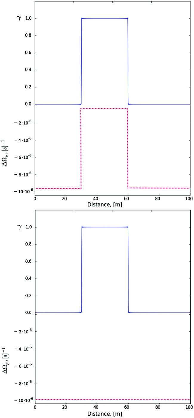
Figure 1. Examples of initial conditions for step profiles both in ΔΩ and γ (top), as used in case III simulations, and those with a flat profile in ΔΩ and step in γ, used in case I and II to initiate a glitch (bottom).
The third setup (case III) is closely related to case II with constant advection, but now the parameter γ is explicitly included in the equation for the lag ΔΩ, which is thus coupled to the evolution of γ. In order to make the problem numerically tractable, the linear term is also excluded and we have an equation in the same form as (24). The initial conditions differ from the previous ones, as the absence of a linear term mean that we cannot trigger a glitch simply with an increase in γ. Rather, we provide an initial step profile for γ and ΔΩ, meaning that the lag is already formed and we force vortices to move as a result of a previous, unspecified, and unpinning event. Examples of these initial conditions are also shown in Figure 1. The equations to solve are
 $$\begin{equation}
\frac{\partial \Delta \Omega }{\partial t} &=& \frac{\mathcal {B}}{{x}_{\mathrm{p}}}{\varpi }_{s} \gamma \Delta \Omega \frac{\partial \Delta \Omega }{\partial \omega }\;,
\end{equation}$$\\
$$\begin{equation}
\frac{\partial \Delta \Omega }{\partial t} &=& \frac{\mathcal {B}}{{x}_{\mathrm{p}}}{\varpi }_{s} \gamma \Delta \Omega \frac{\partial \Delta \Omega }{\partial \omega }\;,
\end{equation}$$\\
 $$\begin{equation}
\frac{\partial \gamma }{\partial t} &=& \frac{\mathcal {B}}{2{x}_{\mathrm{p}}}{\varpi }_{s} {\Omega }_{{\text{init}}}\frac{\partial \gamma }{\partial \omega } \;.
\end{equation}$$
$$\begin{equation}
\frac{\partial \gamma }{\partial t} &=& \frac{\mathcal {B}}{2{x}_{\mathrm{p}}}{\varpi }_{s} {\Omega }_{{\text{init}}}\frac{\partial \gamma }{\partial \omega } \;.
\end{equation}$$
Table 1. Summary of the three different prescriptions that are used to couple vortex motion (evolution of the unpinned vortex fraction γ) and angular momentum exchange (evolution of the lag ΔΩ).
These pairs of equations for the evolution of the lag and the fraction of unpinned vortices for the considered setups have been solved using the Dedalus spectral code (K. J. Burns, G. M. Vasil, J. S. Oishi, D. Lecoanet, B. P. Brown, and E. Quataert, in preparation) as well as with a two-order Godunov finite difference code. Tests of the numerical solution’s accuracy have also been implemented for both codes by means of direct measurements of the velocity of a shock wave in test problems.
We assume a constant mutual friction parameter  $\mathcal {B}$ and assume that the distance travelled by vortices is small compared to the radius ϖs, which we take constant. In a realistic case, mutual friction will depend on density and composition, thus on ϖs, and will be due to different processes in the crust and core, thus depending strongly on the location of our simulation box in the star.
A typical evolution of ΔΩ is shown in Figure 2 for the synchronised velocity case (case I), while the evolution of γ is shown in Figure 3 . The pattern of the process is as follows: an initially flat profile creates a difference in angular velocities, due to the exchange of angular momentum between a normal and a superfluid component, and creates large gradients in ΔΩ. The decrease in lag then spreads out. The typical time for the rise in frequency is less than a second in our setup, but strongly depends on the poorly known mutual friction parameter  $\mathcal {B}$.
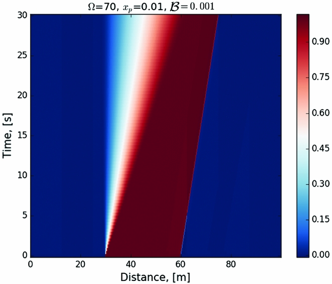
Figure 2. Evolution of γ for case I with step initial condition, as described in the text and seen in Figure 1. The fraction of unpinned vortices decreases, thus approximating a repining process.
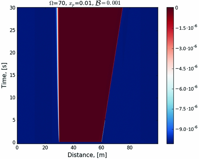
Figure 3. Evolution of ΔΩ for case I with step initial condition, as described in the text and seen in Figure 1.
The evolution of the fraction of unpinned vortices is characterised by a decrease with time, which mimics vortex repining. Note that, in order to solve the equations numerically, artificial dissipation has been introduced.
Let us now turn our attention to the (internal) torque acting on the protons, i.e., on the ‘normal’ component of the star that is coupled to the magnetic field and thus to the observable electromagnetic emission. Locally, the proton angular velocity evolves as
 $$\begin{equation}
{\Omega }_{\mathrm{p}} = {\Omega }_{\mathrm{n}}-\Delta \Omega \;.
\end{equation}$$
$$\begin{equation}
{\Omega }_{\mathrm{p}} = {\Omega }_{\mathrm{n}}-\Delta \Omega \;.
\end{equation}$$
The equation for the proton component for cases I and II in Table 1 is
 $$\begin{equation}
{\Omega }_{\mathrm{p}}= {\Omega }_{\mathrm{n}} - \int \left({\frac{\mathcal {B}}{{x}_{\mathrm{p}}}{\varpi }_{s} \Delta \Omega \frac{\partial \Delta \Omega }{\partial \omega }-2\Omega \Delta \Omega \frac{\gamma \mathcal {B} }{{x}_{\mathrm{p}}}}\right){\text{d}}t\;.
\end{equation}$$
$$\begin{equation}
{\Omega }_{\mathrm{p}}= {\Omega }_{\mathrm{n}} - \int \left({\frac{\mathcal {B}}{{x}_{\mathrm{p}}}{\varpi }_{s} \Delta \Omega \frac{\partial \Delta \Omega }{\partial \omega }-2\Omega \Delta \Omega \frac{\gamma \mathcal {B} }{{x}_{\mathrm{p}}}}\right){\text{d}}t\;.
\end{equation}$$
And for case III is
 $$\begin{equation}
{\Omega }_{\mathrm{p}}= {\Omega }_{\mathrm{n}} - \int \frac{\mathcal {B}}{{x}_{\mathrm{p}}}{\varpi }_{s}\gamma \Delta \Omega \frac{\partial \Delta \Omega }{\partial \omega }{\text{d}}t\;.
\end{equation}$$
$$\begin{equation}
{\Omega }_{\mathrm{p}}= {\Omega }_{\mathrm{n}} - \int \frac{\mathcal {B}}{{x}_{\mathrm{p}}}{\varpi }_{s}\gamma \Delta \Omega \frac{\partial \Delta \Omega }{\partial \omega }{\text{d}}t\;.
\end{equation}$$
In order to consider the motion of a rigid crust, we will average over the interval by integrating between [ϖ1 , ϖ2] that in our case represent the boundaries of our computational domain, i.e., minimum and maximum radial distance in a star at which the evolution of a system is simulated. This leads to
 $$\begin{eqnarray}
\left<{\dot{\Omega }}_{\mathrm{p}}\right> = \left<{\dot{\Omega }}_{\mathrm{n}}\right> - \frac{1}{{\varpi }_{1}-{\varpi }_{2}}\int _{{\varpi }_{1}}^{{\varpi }_{2}}\left(\frac{{\varpi }_{s}\mathcal {B}}{{x}_{\mathrm{p}}} \Delta \Omega \frac{\partial \Delta \Omega }{\partial \omega }\right.\nonumber \\
&&-\, \left.2\Omega \Delta \Omega \frac{\gamma \mathcal {B} }{{x}_{\mathrm{p}}}\right){\text{d}}\omega \;,
\end{eqnarray}$$
$$\begin{eqnarray}
\left<{\dot{\Omega }}_{\mathrm{p}}\right> = \left<{\dot{\Omega }}_{\mathrm{n}}\right> - \frac{1}{{\varpi }_{1}-{\varpi }_{2}}\int _{{\varpi }_{1}}^{{\varpi }_{2}}\left(\frac{{\varpi }_{s}\mathcal {B}}{{x}_{\mathrm{p}}} \Delta \Omega \frac{\partial \Delta \Omega }{\partial \omega }\right.\nonumber \\
&&-\, \left.2\Omega \Delta \Omega \frac{\gamma \mathcal {B} }{{x}_{\mathrm{p}}}\right){\text{d}}\omega \;,
\end{eqnarray}$$
and
 $$\begin{equation}
\left<{\dot{\Omega }}_{\mathrm{p}}\right> = \left<{\dot{\Omega }}_{\mathrm{n}}\right> - \frac{1}{{\omega }_{1}-{\omega }_{2}}\int _{{\omega }_{1}}^{{\omega }_{2}}{\frac{\mathcal {B}}{{x}_{\mathrm{p}}}{\varpi }_{s}\gamma \Delta \Omega \frac{\partial \Delta \Omega }{\partial \omega }}{\text{d}}\omega \;.
\end{equation}$$
$$\begin{equation}
\left<{\dot{\Omega }}_{\mathrm{p}}\right> = \left<{\dot{\Omega }}_{\mathrm{n}}\right> - \frac{1}{{\omega }_{1}-{\omega }_{2}}\int _{{\omega }_{1}}^{{\omega }_{2}}{\frac{\mathcal {B}}{{x}_{\mathrm{p}}}{\varpi }_{s}\gamma \Delta \Omega \frac{\partial \Delta \Omega }{\partial \omega }}{\text{d}}\omega \;.
\end{equation}$$
In this initial calculation, we neglect  $\left<{\dot{\Omega }}_{\mathrm{n}}\right>$, in the assumption that the proton fluid has a smaller moment of inertia and thus the background average neutron rotation rate does not change very much compared to the proton rotation rate, i.e., $|\left<{\dot{\Omega }}_{\mathrm{p}}\right>| >> |\left<{\dot{\Omega }}_{\mathrm{n}}\right>|$. This is not always the case, however, and a more realistic calculation should retain both terms (Haskell et al. Reference Haskell, Pizzochero and Sidery2012).
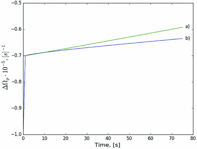
Using the previously obtained results for the lags ΔΩ, we average over the computational domain for each setup and show the results in Figure 4. The comparison of the related scenarios for constant advection are shown in Figure 5.
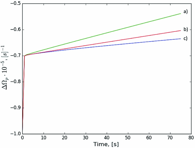
Figure 4. Comparison of the charged component evolution for the different setups. (a) Synchronised velocity setup (case I): [(41), (42)] with an initially flat profile for ΔΩ and step in γ; (b) Constant advection setup (case III) [(46), (47)] with initial step profiles in both ΔΩ and γ; (c) Synchronised velocity (case I) with artificially decreased speed of free vortex propagation ( $\mathcal {B}$ reduced as described in the text).

Generally, for the reference value  $\mathcal {B}=10^{-3}$ as well as for the lower value $\mathcal {B}=10^{-4}$, the behaviour of the ‘normal’ component is characterised by a rapid exponential rise, on timescales of seconds, followed by a slower, apparently linear, increase in frequency on timescales of a minute. This behaviour is, in fact, suggestive of what was observed for the 1989 glitch of the Crab pulsar, in which a fast and unresolved rise was followed by a slower component (Lyne, Smith, & Pritchard Reference Lyne, Smith and Pritchard1992).
As can be seen from Figures 4 and 5, the rise time for the three major setups is almost the same, while there are differences in the linear responses. However, the differences in frequency and frequency derivative are still small, and of order of 30% for the frequency derivative, indicating that in the study of the short-term rise and post-glitch behaviour, the choice of setup does not strongly influence the conclusions.
5.2. Glitch precursors
We now discuss how differences in pinning strengths in the neutron star crust can influence the evolution of the frequency, and in particular whether unpinning in lower strength pinning regions can trigger unpinning and glitches in regions with stronger pinning and thus larger lags. In other words, we are interested in examining whether smaller unpinning events, that may show up simply as changes in spin-down rate, rather than steps in frequency, could be glitch precursors, as observed, for example, in the pulsar J0537–6910 (Middleditch et al. Reference Middleditch, Marshall, Wang, Gotthelf and Zhang2006).
To do this, let us consider the evolution of a system with the lag between the normal and the superfluid component that is not simply a step but a sequence of steps. Initial conditions for this case are shown in Figure 6. Different lags ΔΩ correspond to a different pinning strength, as stronger pinning leads to a larger critical lag.
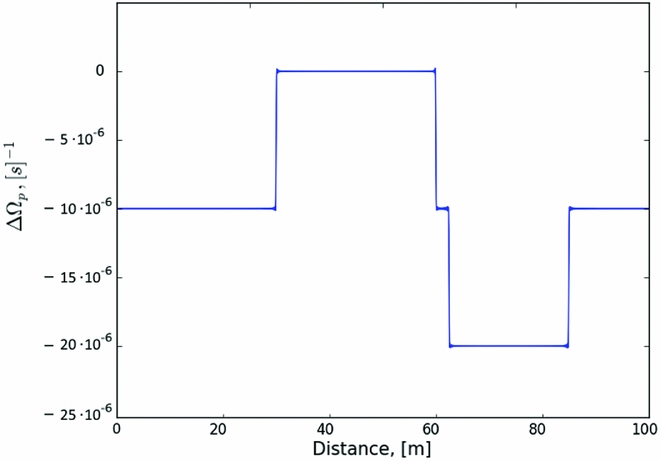
Figure 6. Initial condition for the lag with a sequence of steps, physically corresponding to different pinning strengths.
To study the evolution, we use the equations from case III, i.e., [(46), (47)], with initial conditions for γ being a step located at the same distance and with the same width as in Figure 1. Note that the lag in the second region is twice that in the first (i.e., the pinning is twice as strong). Larger differences can be expected in neutron star crusts, but cannot be treated in our current numerical setup. The results of solving (46) and (47) are in Figure 7 for the evolution of the lag ΔΩ, and in Figure 8 for the evolution γ.
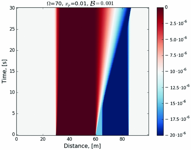
Figure 7. Evolution of the lag ΔΩ for the initial conditions in Figure 6.
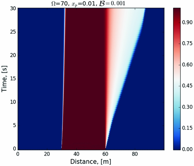
Figure 8. Evolution of the parameter γ for the initial conditions in Figure 6.
A propagating wave begins to travel due to the unpinned vortices. When reaching the region with a higher lag, the transfer of angular momentum is much more effective and this results in increase of rotational rate as seen in the evolution of the charged component. Due to the presence of regions with a non-uniform distribution of pinning forces, and thus of lag between the normal and the superfluid component, in real NSs a more complex pattern is likely to appear. The fraction of free vortices, in turn, goes through two transitions. The first transition occurs when free vortices reach the region with a higher lag, where the amount of free vortices that are able to continue moving further decreases. The second transition occurs when vortices pass this region. Their amount then decreases with a constant rate.
The evolution of the charged component is shown in Figure 9. Unlike the other setups now, the initial rise time is much longer. When free vortices reach the region with a higher lag, the slope increases and decreases again after passing the region. This means that amplification of the initial rise is possible if in the outer region the pinning force is stronger.
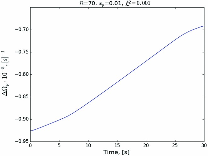
Figure 9. Evolution of the lag ΔΩ for initial conditions in Figure 6. The difference in critical lags leads to an initial slower rise, followed by a faster increase in frequency when the unpinning front reaches the stronger pinning region. Even larger differences in critical lag (and equivalently pinning force) could lead to a faster and larger glitch after the initial precursor, but are numerically intractable in our setup.
As a result, the star’s angular velocity may change not only abruptly, showing a glitch-like rise, but also more gradually, depending on local properties of the region, i.e., the distribution of areas with uneven pinning but also the local value of the mutual friction and the moment of inertia of the fluid. In general, our results indicate that an initial increase in the spin-down rate (decrease in absolute value) may be the precursor of a larger glitch, although the differences in pinning required for this scenario are larger than those that our numerical setup allows. We are thus unable to simulate physically realistic sizes and timescales.
This behaviour, however, is similar to what has been observed in pulsar J0537–6910 (Middleditch et al. Reference Middleditch, Marshall, Wang, Gotthelf and Zhang2006; Ferdman et al. Reference Ferdman, Archibald, Gourgouliatos and Kaspi2018), where the preglitch behaviour exhibits brief ‘upticks’ and ‘downticks’ in  $\dot{\nu }$ of varying amplitudes and durations. The timescales are different from those that we simulate, due to our numerical limitations. However, our results, although they depend on poorly known physical quantities in the crust of the star, indicate that it is possible that the same process in a NS may lead to different phenomena. In the case presented here, the interaction between the superfluid and the normal component gives a rise to a glitch precursor, while the same process in an isolated strong pinning region leads to a standard glitch.
5.3. Frequency decrease and antiglitches
The non-linear evolution we consider can, however, lead to other surprising results in the framework of the standard glitch model. In particular, we find setups in which not only an increase, but also a decrease in a star’s angular velocity can be obtained. To do this, we study the evolution of a system with step initial conditions using the setup in case III, corresponding to equations (46) and (47). Initial conditions for two cases are shown in Figure 10.
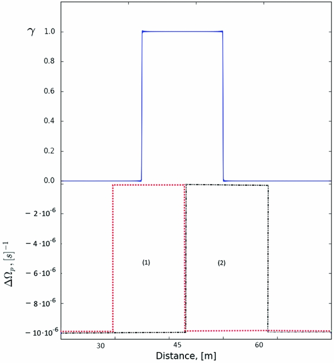
Figure 10. Initial conditions for γ and ΔΩ for the antiglitch test cases described in the text. Two cases are shown: (1) conditions leading to and increase of the angular velocity; (2) conditions leading to a decrease of the angular velocity, or ‘antiglitch’.
The difference between the two setups is that in the first case the region with null lag is located ‘behind’ the region with free vortices and these regions partially coincide while in the second case the null-lag region is located further out than the front. Results for this case are shown in Figure 11.
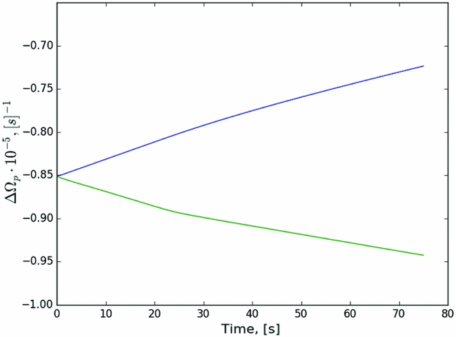
Figure 11. Evolution in time of the angular velocity of a charged component for a glitch–‘antiglitch’ test. The blue rising curve corresponds to the glitch-like rise, the green decreasing curve to the antiglitch-like behaviour.
As can be seen from the figure, unpinned vortices in the area behind the zero lag region start to exchange angular momentum, which tends to increase the angular velocity. However, propagation tends to decrease the extent of the coupled region at a faster rate, resulting in an ‘anti-glitch’, i.e., a local decrease of angular velocity. This behaviour is intriguing, given observations of such antiglitches in magnetars (Archibald et al. Reference Archibald2013). However, since the decrease in frequency is the result of a competition of process, it is possible that the overall antiglitch behaviour is the consequence of our particular setup. As for the influence of the numerical dissipation, several tests have been made in order to study the changes of the ‘antiglitch’ behaviour appearance as well as the time of rise. It was found that it has minimal impact on the results, and the feature is robust for our setup. However, further investigation in a more realistic scenario will be required to determine whether this evolution is physically significant.
Other initial conditions, in fact, result in much more predictable evolutions and show an increase of angular velocity, as shown in Figure 11 as a blue curve, while the ‘antiglitch’ is shown as green curve.
Let us study in detail the evolution of the solution where the ‘antiglitch’ appears. For this, we show four snapshots for γ and ΔΩ on Figure 12.
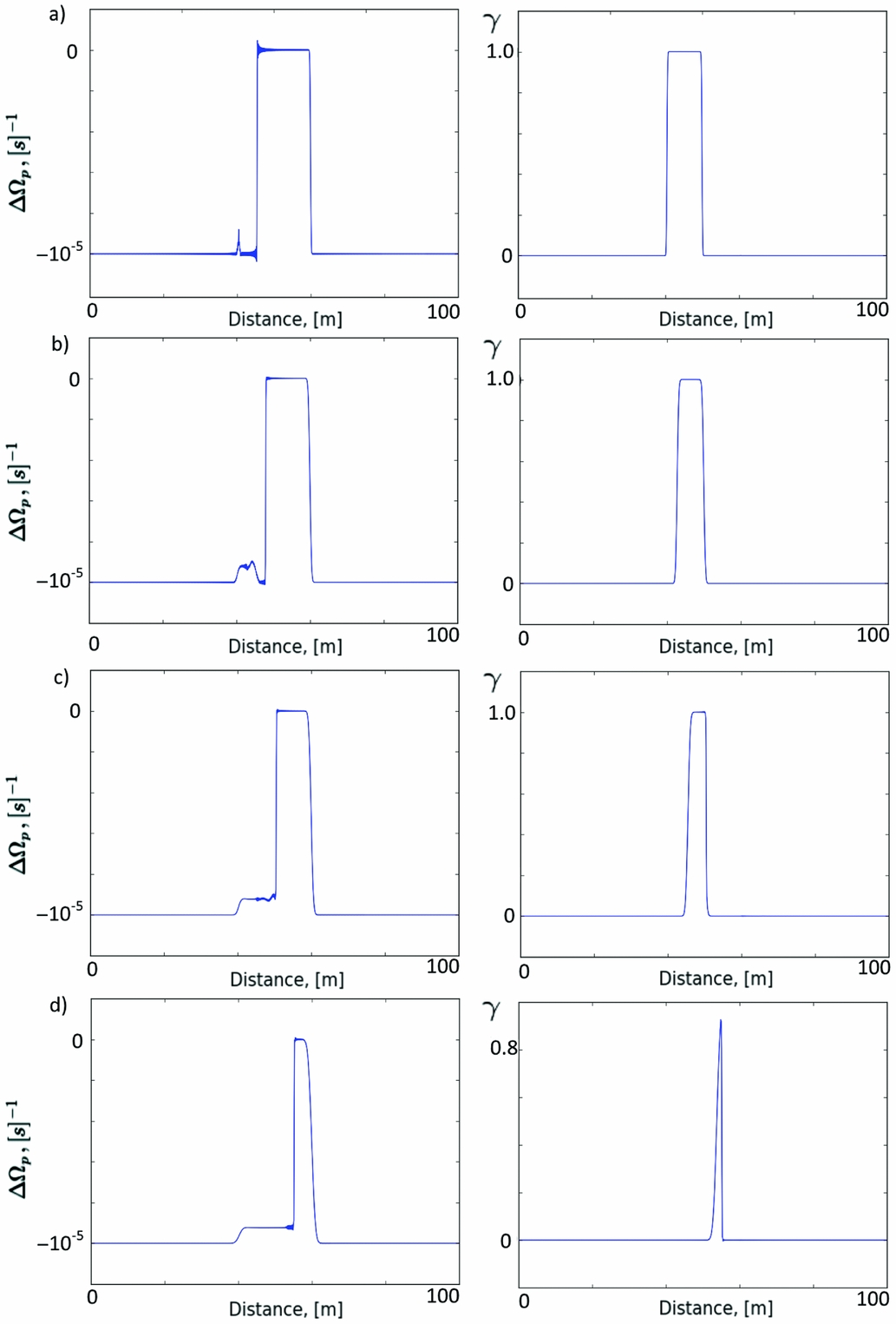
Figure 12. Snapshots of evolution in time for ΔΩ (left column) and γ (right column) (a) After 1 s; (b) after 6 s; (c) after 12 s; (d) after 30 s.
Initially, unpinned vortices form a small peak in ΔΩ behind the main region of the lag. This peak grows with time until it reaches the main region with zero lag. Next, these two regions start to interact, forcing the initial region with vortices to decrease in size and move. Further interaction makes both regions move, γ decrease and an unpinning wave propagate. The overall outcome, whether an increase or decrease in frequency, is thus sensitive to the timescale on which these processes occur and the speed of propagation of γ.
6 PARAMETER STUDY
To study the influence of the different parameters on the evolution of the solution, we first change the mutual friction, i.e., the  $\mathcal {B}$ parameter. In a realistic star, this parameter depends on density, and will thus depend on the location of the computational box in the NS. Since we take the mutual friction to be constant, it represents the averaged value over the computational domain, i.e., over the path of vortex movement. Decreasing the mutual friction will generally increase the timescale for the rise, while higher mutual friction leads to a faster glitch, for a fixed initial setup.
The dependance is intuitively correct since the mutual friction is the mechanism that is responsible for an angular’s momentum transfer strength, it is a ‘bridge’ between the normal and the superfluid component, and the behaviour can easily be understood from equation (21) for the coupling timescale between components, if we neglect non-linear terms. The consequences of the mutual friction variations are shown in Figure 13 for case II as a representative of a non-constant advection family and in Figure 14 for case I with constant advection.

Figure 13. Influence of the mutual friction parameter  $\mathcal {B}$ on the speed of rise for case II. (a) $\mathcal {B} = {10}^{-3}$; (b) $\mathcal {B} = {10}^{-4}$; (c) $\mathcal {B} = {10}^{-5}$.
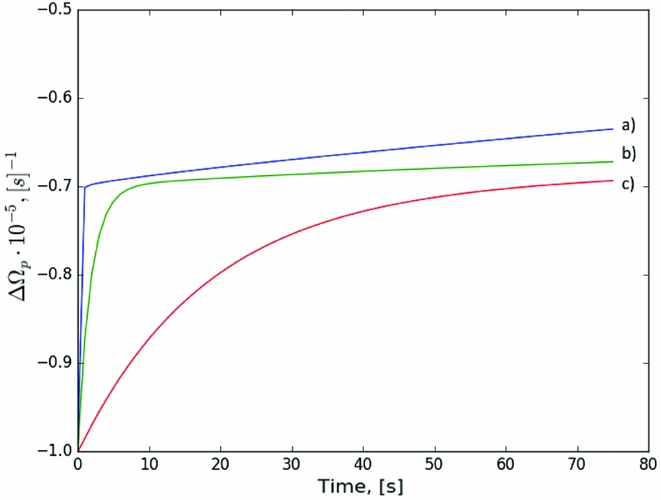
Figure 14. Influence of the mutual friction parameter  $\mathcal {B}$ on the speed of rise for case I. (a) $\mathcal {B} = {10}^{-3}$; (b) $\mathcal {B} = {10}^{-4}$; (c) $\mathcal {B} = {10}^{-5}$.
Note that  $\gamma \mathcal {B}$ is the parameter that affects the character of a glitch. Its evolution leads, for example, to different kinds of relaxation even in a single pulsar, given that in a realistic system it is not constant in time (due to vortex pinning and unpinning) or constant along the path of vortex movement (Haskell & Antonopoulou Reference Haskell and Antonopoulou2014).
Next, let us study the influence of the angular frequency of a star. In all of the simulations, the angular frequency is initially equal to 70 s−1 which is approximately equal to the Vela pulsar’s angular velocity. In order to see how the unpinning wave propagation reacts, we experiment with changing it to 7 s−1. Results are shown on Figure 15. As expected from the linear analysis in (21), decreasing the angular velocity of a star increases the rise time but does not strongly affect the results in the non-linear regime.
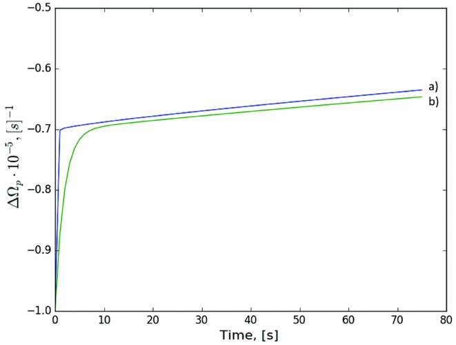
Figure 15. Influence of the angular frequency Ω of a star on the charged component evolution for constant advection, i.e., case I: (a) Ω = 70 s−1, (b) Ω = 7 s−1.
Changing the proton fraction x p acts as a simple rescaling of the mutual friction parameter  $\mathcal {B}$ in our simple setup, and thus does not significantly affect the results for reasonable values of the parameter in the crust.
7 CONCLUSIONS
In this paper, we have outlined a formalism for simulating the motion of superfluid vortex over-densities and fronts in hydrodynamical two-fluid simulations of pulsar glitches. We have shown that accounting explicitly for the differential rotation that is built up due to vortex accumulation introduces additional non-linear terms in the evolution equations for the lag ΔΩ, which allow for travelling waves (‘unpinning’ waves) as solutions. The observational consequence of this setup is that coupling between the normal and superfluid components of the neutron star, mediated by vortex motion, can lead not only to exponential terms in the evolution of a pulsar’s frequency, but also linear terms, and generally slower, longer term variations in the spin frequency of a neutron star.
We take our model one step further and introduce an additional parameter to the evolution, namely the fraction of free vortices in the system, γ. This parameter encodes the sub-grid physics of vortex motion that is not resolved on a hydrodynamical level, and depends on the complex quantum mechanical statistical processes that govern vortex interactions at a microscopic level. While microphysical simulations have been relatively successful in investigating the relation between pulsar glitches and SOC (Warszawski & Melatos Reference Warszawski and Melatos2011; Haskell & Melatos Reference Haskell and Melatos2015) in small systems, or pinning of a vortex to a single defect (Wlazłowski et al. Reference Wlazłowski, Sekizawa, Magierski, Bulgac and Forbes2016), they are still not at the level where contact can be made with large-scale descriptions. We thus propose three phenomenological models for vortex motion, all of which mimic advection of free vortices together with propagating fronts in the lag between the normal component and the superfluid neutrons.
We study the evolution of the lag ΔΩ and the free vortex fraction γ in several setups for all three our prescriptions for varying mutual friction parameters  $\mathcal {B}$ and rotation rates Ω. The main conclusion is that localised unpinning leads to an initial rapid rise, on the timescale of seconds or less for mutual friction parameters $\mathcal {B}>10^{-4}$, as one may expect due to electron scattering of magnetised vortex cores in the presence of superconducting protons (Alpar et al. Reference Alpar, Langer and Sauls1984b), or due to Kelvin waves as the vortices move past nuclear clusters in the crust (Jones Reference Jones1992; Epstein & Baym Reference Epstein and Baym1992). This phase is, however, generally followed by a slower, quasi-linear rise on timescales of a minute, which is similar to what was observed in the 1989 glitch of the Crab pulsar (Lyne et al. Reference Lyne, Smith and Pritchard1992). Overall, the prescription we use for motion of the vortex fraction has little influence on the exponential rise, which is mainly due to the linear terms, but impacts on the slower long-term evolution. Nevertheless, the evolution of the normal component frequency is qualitatively similar, with only modest differences in rotational rates and frequency derivatives, between the three cases, which gives us confidence that our conclusions are robust and do not depend strongly on how we approximate the sub-grid physics of vortex motion.
We have also investigated how changes in pinning strength, approximated by different initial conditions for the lag, can impact the evolution of the frequency and the glitch. We find that if there are regions in which pinning decreases with density, as one expects in the deep crust (Seveso et al. Reference Seveso, Pizzochero, Grill and Haskell2016), then an initial unpinning event may lead to a slow change in frequency as a precursor of a larger glitch, triggered when the unpinning front reaches the stronger pinning region. Such precursor events may, in fact, have been observed before a number of glitches in pulsar J0537–6910 (Middleditch et al. Reference Middleditch, Marshall, Wang, Gotthelf and Zhang2006; Ferdman et al. Reference Ferdman, Archibald, Gourgouliatos and Kaspi2018), where ‘upticks’ and ‘downticks’ in  $\dot{\nu }$ of varying amplitudes and durations were observed prior to several glitches.
We also find specific setups in which vortex motion can lead to a decrease in frequency, or an antiglitch, such as that observed in the magnetar 1E 2259+586 (Archibald et al. Reference Archibald2013). This behaviour is intriguing, as it would provide an explanation for this phenomenon in the standard glitch model [see also Kantor & Gusakov (Reference Kantor and Gusakov2014) for an alternative approach]. In our setup, the feature is robust to changes in numerical dissipation, and does not appear to be a numerical artefact. Nevertheless, a more detailed study in a more realistic setup is necessary to understand whether such an evolution is physically significant and would occur in a neutron star.
Despite the uncertainties, both due to the implementation of vortex motion, and poorly constrained physical parameters in the interior of the neutron stars, our simple models highlight the importance of allowing for vortex motion and accumulation in hydrodynamical simulations, as this allows for new and qualitatively different behaviour before, during and after a glitch. On the other hand, our models are also further confirmation that the large-scale response of the star strongly impacts on conclusions drawn from small-scale vortex dynamics alone, as was already shown to be the case for size and waiting time distributions (Haskell Reference Haskell2016). Future work should thus focus on further bridging the gap in scales between microscopic quantum mechanical simulations of vortex motion and large-scale hydrodynamical models of superfluid neutron stars.
ACKNOWLEDGEMENTS
We acknowledge support from the Polish National Science Centre (SONATA BIS 2015/18/E/ST9/00577, P.I.: B.Haskell) and from the European Union’s Horizon 2020 research and innovation programme under grant agreement no. 702713. Partial support comes from NewCompStar, COST Action MP1304.
We thank Varadarajan Parthasarathy and Morgane Fortin for constructive discussions.