


1. Introduction
In the past three decades, thousands of exoplanets have been revealed (http://exoplanets.org), providing significant statistics on worlds outside our own and a new frontier for modern astronomy to explore. While most detections have been achieved through indirect techniques, there is a growing need to observe the direct light of these worlds, not generally achievable with the currently available instruments (although some outlier systems with favourable configuration have been detected). Of primary interest is the study of temperate terrestrial planets in configurations similar to Earth, which comprise the most obvious candidates to host ‘life as we know it’. There is now worldwide momentum behind the growing field of research to develop the technology and instrumentation to reach this challenging, yet not unachievable goal. The direct detection of exoplanetary light is difficult for three main reasons. Firstly, the habitable zone orbits occupied by distant worlds (and particularly Earth analogues) are tiny when viewed from Earth and require high angular resolution (of order of 10’s to 100’s of milli-arcseconds for nearby systems). Second, light from the planet, either reflected starlight or intrinsic emission, is inherently faint, requiring acute sensitivity. Lastly, even with the most sensitive instrument, the planet light is outshone (by many orders of magnitude) by the light from the host star(s). Typical contrast ratios of the order of $10^{-10}$
are required for directly observing reflected light from an Earth-like planet around a Sun-like star in the near infrared (Guyon et al. Reference Guyon, Martinache, Cady, Belikov, Balasubramanian, Wilson, Clergeon, Mateen, Ellerbroek, Marchetti and Vèran2012; Schworer, Guillaume, & Tuthill 2015).
$10^{-10}$
are required for directly observing reflected light from an Earth-like planet around a Sun-like star in the near infrared (Guyon et al. Reference Guyon, Martinache, Cady, Belikov, Balasubramanian, Wilson, Clergeon, Mateen, Ellerbroek, Marchetti and Vèran2012; Schworer, Guillaume, & Tuthill 2015).
Optical stellar interferometry offers an answer to both the angular resolution and contrast problem. By coherently superposing the starlight of two (or several) apertures, whose separations correspond to different spatial frequencies, optical interference is obtained which can be interpreted in terms of the spatial geometry of the source (van Cittert Reference van Cittert1934; Zernike Reference Zernike1938). The angular resolution is typically given as $\lambda/B$
(Monnier Reference Monnier2003), with
$\lambda/B$
(Monnier Reference Monnier2003), with $\lambda$
the wavelength of the light observed and B the baseline, or separation between apertures, spanning up to hundreds of metres for ground-based interferometers. By adding a phase delay of
$\lambda$
the wavelength of the light observed and B the baseline, or separation between apertures, spanning up to hundreds of metres for ground-based interferometers. By adding a phase delay of $\pi$
in one of the interferometric arms, light from an on-axis source is destructively interfered leaving a faint off-axis companion unaffected. By rotating the baseline, the amplitude of the interference is modulated and spatial information of the planet(s), such as its orbit, can be retrieved. This is the principle of nulling interferometry first proposed by Bracewell (Reference Bracewell1978) and illustrated in Figures 1 and 2. The light can then be fed into further downstream instruments such as spectrographs, to study the chemical composition of the companion’s atmosphere and surface. In a visionary future implementation of such technologies, weather, vegetation, seasons, and biological life may be inferred (Fujii et al. Reference Fujii, Kawahara, Suto, Taruya, Fukuda, Nakajima and Turner2010; Snellen Reference Snellen2014; Seager, Bains, & Petkowski Reference Seager, Bains and Petkowski2016).
$\pi$
in one of the interferometric arms, light from an on-axis source is destructively interfered leaving a faint off-axis companion unaffected. By rotating the baseline, the amplitude of the interference is modulated and spatial information of the planet(s), such as its orbit, can be retrieved. This is the principle of nulling interferometry first proposed by Bracewell (Reference Bracewell1978) and illustrated in Figures 1 and 2. The light can then be fed into further downstream instruments such as spectrographs, to study the chemical composition of the companion’s atmosphere and surface. In a visionary future implementation of such technologies, weather, vegetation, seasons, and biological life may be inferred (Fujii et al. Reference Fujii, Kawahara, Suto, Taruya, Fukuda, Nakajima and Turner2010; Snellen Reference Snellen2014; Seager, Bains, & Petkowski Reference Seager, Bains and Petkowski2016).
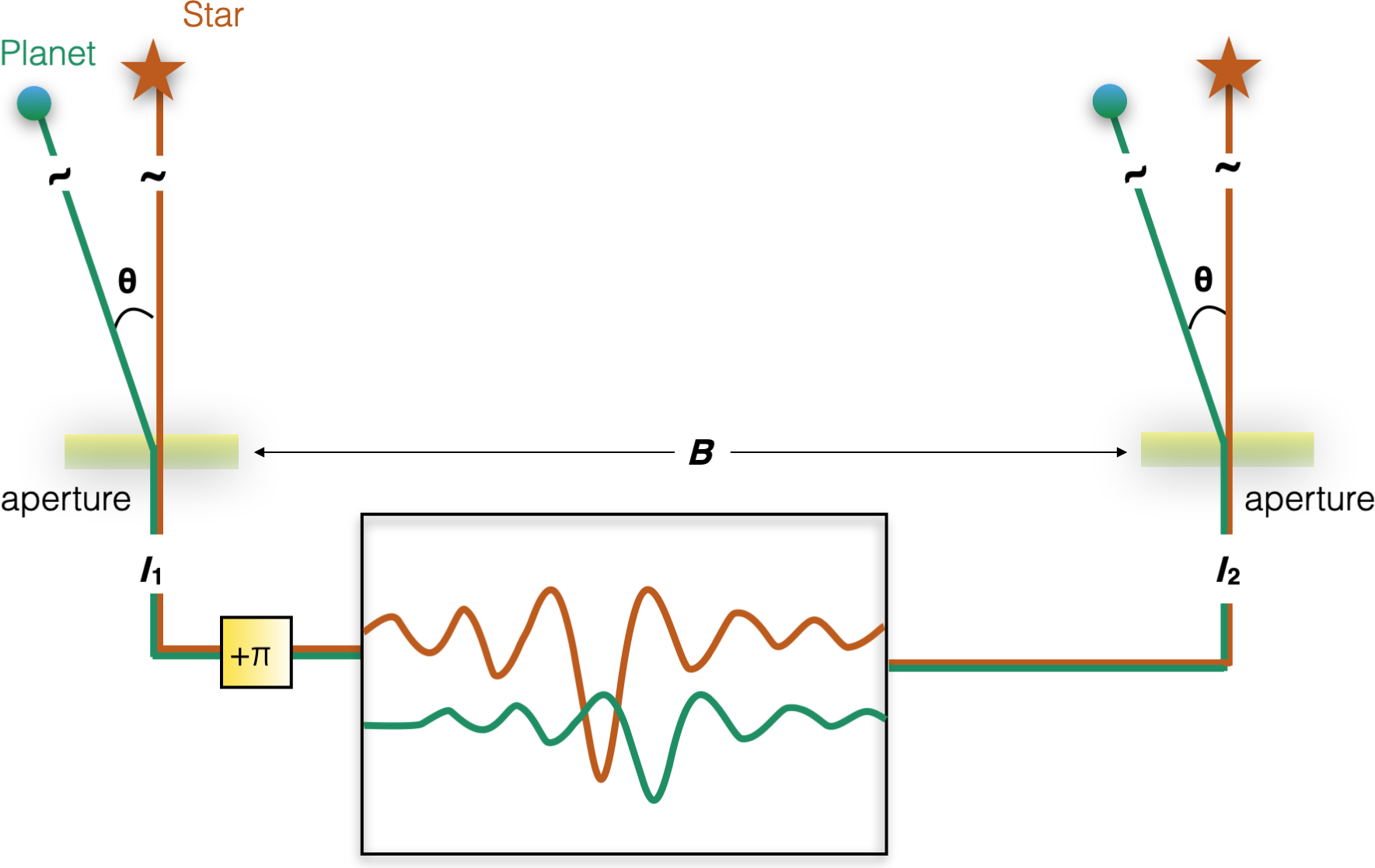
Figure 1. Illustration of the principle of nulling interferometry. The light of a star is collected by two apertures separated by a baseline B. A phase delay of $\pi$
is introduced into one of the arms to produce a deep central minimum in the interference of the light beams. If a planet orbits the star at an angular separation of
$\pi$
is introduced into one of the arms to produce a deep central minimum in the interference of the light beams. If a planet orbits the star at an angular separation of $\theta$
, its light enters the instrument off-axis introducing a further delay of
$\theta$
, its light enters the instrument off-axis introducing a further delay of $B\sin(\theta)$
. As a consequence, the starlight is locally highly suppressed while the planet light is not.
$B\sin(\theta)$
. As a consequence, the starlight is locally highly suppressed while the planet light is not.
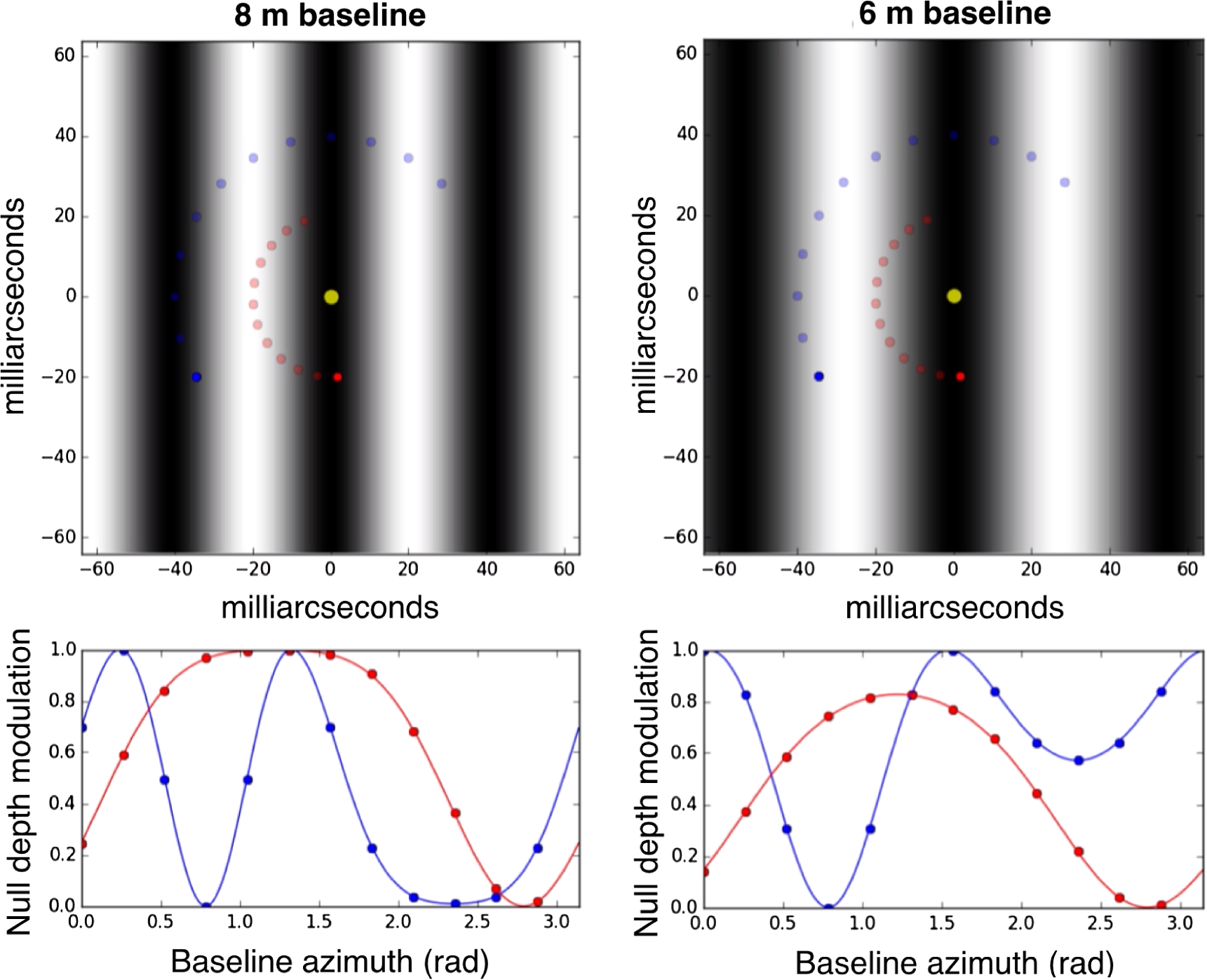
Figure 2. Null depth measures the extinction of the starlight and relates directly to the contrast of the fringe. In the top panel, the fringe pattern is projected onto the plane of observation. The fringe spacing depends on the baseline. In the bottom panel, the null depth is modulated as two planets (blue and red) rotate around a centrally nulled star and traverse the projected fringe pattern.
Another technique being developed to directly image exoplanets is coronagraphy, which uses a physical mask to block the starlight. In recent years, coronagraphy has demonstrated detection of large, bright, and widely separated self-luminous planetary companions (Kalas et al. Reference Kalas2008; Macintosh et al. Reference Macintosh2015; Zurlo et al. Reference Zurlo2016; Mesa et al. Reference Mesa2019) but is limited by the inner working angle (the spatial separation from the centre of the field of view over which off-axis objects would have a 50% throughput through the coronagraph). The emergence of nulling interferometry is more a complement rather than a competitor to coronagraphy as it is capable of working well within the inner working angle of a coronagraph, making it well suited for observing planets in relatively close (AU scale) orbits. This makes it an ideal technology for temperate orbit terrestrial planets.
Nulling interferometry was proposed as a suitable technology for deployment in space, for the Darwin mission from ESA (Léger et al. Reference Léger, Mariotti, Mennesson, Ollivier, Puget, Rouan and Schneider1996), the Terrestrial Planet Finder from NASA (Beichman, Woolf, & Lindensmith Reference Beichman, Woolf and Lindensmith1999) and the ESA space mission LIFE, currently being reviewed (Quanz et al. Reference Quanz, Kammerer, Defrère, Absil, Glauser and Kitzmann2018). The first two missions were eventually cancelled due partly to the premature state of the required technologies at the time such as the accurate formation flying of satellites. However, NASA funded several pathfinder programmes: the Keck Interferometric Nuller (KIN) (Colavita et al. Reference Colavita and Reasenberg1998; Serabyn et al. Reference Serabyn, Mennesson, Colavita, Koresko and Kuchner2012) and the Large Binocular Telescope Interferometer (LBTI) (Angel & Woolf Reference Angel and Woolf1997) to characterise the degree to which exozodiacal light acts to contaminate signals from exoplanets. LBTI has demonstrated extinction ratios of $\ {\sim}3 \times 10^{-4}$
in the N band from 8 to 13
$\ {\sim}3 \times 10^{-4}$
in the N band from 8 to 13 $\unicode[Times]{x03BC}$
m (Ertel et al. Reference Ertel2020) using conventional bulk optics. Another nuller instrument is the Palomar Fiber Nuller (PFN) demonstrated extinction ratios of a few 10–4 in the K band centered at 2.15
$\unicode[Times]{x03BC}$
m (Ertel et al. Reference Ertel2020) using conventional bulk optics. Another nuller instrument is the Palomar Fiber Nuller (PFN) demonstrated extinction ratios of a few 10–4 in the K band centered at 2.15 $\unicode[Times]{x03BC}$
m and recently the detection of a faint companion (Serabyn et al. Reference Serabyn, Mennesson, Martin, Liewer and Kühn2019; Mennesson et al. Reference Mennesson, Serabyn, Hanot, Martin, Liewer and Mawet2011).
$\unicode[Times]{x03BC}$
m and recently the detection of a faint companion (Serabyn et al. Reference Serabyn, Mennesson, Martin, Liewer and Kühn2019; Mennesson et al. Reference Mennesson, Serabyn, Hanot, Martin, Liewer and Mawet2011).
Novel and prolific photonic technologies available can deliver the fine manipulation of light. Direct applicability to the telecommunication industry has driven commercial development to a mature state for photonic devices, particularly around the 1 500-nm spectral region. By harnessing this capability for astronomical instrumentation, a new field of astrophotonics has emerged (Bland-Hawthorn & Kern Reference Bland-Hawthorn and Kern2009). The potential for the specific application to stellar interferometry was recognised much earlier (Froehly Reference Froehly1981; Coudé du Foresto Reference Coudé du Foresto1997; Coudé du Foresto et al. Reference Coudé du Foresto, Perrin, Ruilier, Mennesson, Traub, Lacasse and Reasenberg1998). Single-mode fibers act as spatial filters selectively rejecting high-order wavefront distortions (such as those induced by the turbulent atmosphere), increasing the coherence and therefore the contrast of the fringe (Mennesson, Ollivier, & Ruilier Reference Mennesson, Ollivier and Ruilier2002). This implies higher levels of starlight suppression for nulling interferometry.
More recent progress in photonics presents new ways of guiding light through solid devices, a field known as integrated optics. These devices are powerful as they can be designed to implement micrometre accuracy light circuits, integrating many photonic devices such as light guides, splitters, and couplers into one single device (Kern et al. Reference Kern, Berger, Haguenauer, Malbet and Perraut2001). Furthermore, these devices offer high thermal and mechanical stability as well as a convenient and robust miniature format.
With the lithographic technique, waveguides are sculpted on top of a substrate by edging the surface in different steps with masks. Alternatively, a high repetition pulsed laser is focused inside the bulk of a material inducing a permanent change of refractive index and is translated smoothly drawing the waveguides, known as the direct-write technique. On one hand, devices fabricated by lithography have been utilised to simultaneously combine several apertures in long baseline interferometry (Gravity Collaboration Reference Gravity2017). Lithography is an expensive process with long-lead fabrication times (of the order of months) but has demonstrated devices working over a broad wavelength range (Ghasempour et al. Reference Ghasempour, Leite, Reynaud, Marques, Garcia, Alexandre and Moreira2009; Labadie & Wallner Reference Labadie and Wallner2009). On the other hand, direct-written devices can be fabricated in a matter of minutes in a cost-effective manner and can produce three-dimensional circuit designs, all of which allows for greater flexibility in design and testing (Arriola et al. Reference Arriola, Gross, Jovanovic, Charles, Tuthill, Olaizola, Fuerbach and Withford2013). The main drawback of the direct-write process is a more restricted operational spectral range. For this reason, it has not yet been fully exploited in astronomy.
Guided Light Interferometric Nulling technology (GLINT) is an ongoing programme to employ these new photonic capabilities, in particular for high angular resolution and high-contrast imaging. GLINT South is one of two testbed instruments built to demonstrate and develop the direct-write technique for nulling interferometry.
In Section 2 of this paper, the GLINT South instrument is presented, including a description of the nulling chip, the injection control systems, and a short discussion of the alignment process. Section 3 delves into the details of a statistical model to fit GLINT nulled data. In Section 4, the instrument is characterised in the laboratory. Section 5 presents the on-sky results of the testing campaign at the Anglo-Australian Telescope (AAT), starting from the quantification of the starlight injection through the control systems, to nulling of the starlight on a selected bright Mira variable stars. Section 6 offers conclusions and a discussion of the outcomes in the context of future steps in high-contrast detection.
2. The GLINT South instrument
GLINT began with the idea of developing an instrumental solution for imaging exoplanets using 3D integrated optics with the direct-write technology. Dragonfly was the very first precursor instrument (Jovanovic et al. Reference Jovanovic2012) to be built by our group to test the technology. It employed a three-dimensional direct-write integrated optics chip to remap eight sub-apertures of a telescope into a linear array (Charles et al. Reference Charles2012). The sub-apertures were then combined inside a lithographic chip. Following its successful demonstration on sky, a new annealing process for the direct-write technique was developed, producing low-loss waveguides (with throughput >80%) with low birefringence (Arriola et al. Reference Arriola, Gross, Jovanovic, Charles, Tuthill, Olaizola, Fuerbach and Withford2013). A new generation of direct-write chips was then designed and fabricated for nulling interferometry, with one of them now at the heart of GLINT.
The chip (displayed in Figure 3) combines the light from two separate apertures on a telescope. The input waveguides first undergo a ‘side step’: a strategy devised to avoid interference at the outputs with uncoupled light propagating through the bulk (Norris et al. Reference Norris2014). Each waveguide then goes through a y-junction that sends 1/3 of the light to the photometric outputs to monitor the incoming fluxes. The two other branches of the y-splitters are brought in close proximity to form a directional coupler where the modes are mixed by evanescent coupling of the electromagnetic fields, generating interference. The coupler has been designed so that the two interferometric outputs have a $\pi$
-phase difference between them. When light injected has a
$\pi$
-phase difference between them. When light injected has a $\frac{\pi}{2}$
phase offset between the beams, one interferometric output measures the ‘bright’ fringe, while the other measures the ‘dark’ fringe.
$\frac{\pi}{2}$
phase offset between the beams, one interferometric output measures the ‘bright’ fringe, while the other measures the ‘dark’ fringe.
The GLINT programme has two prototype instruments. One is now permanently installed at the 8-m Subaru Telescope in Hawaii, (Norris et al. Reference Norris2020; Martinod et al. Reference Martinod2021a) referred as GLINT (or GLINT North), and one as a testbed in Australia, referred to as GLINT South (Lagadec et al. Reference Lagadec2018). This paper concentrates on the latter. With no world-class adaptive optics (AO) equipped telescopes on the Australian mainland, GLINT South offers a platform for testing, characterising, and interfacing the direct-written chips as they are developed into more complex three-dimensional geometries and wider bandwidths. GLINT South is currently the only nuller working in the Southern hemisphere.
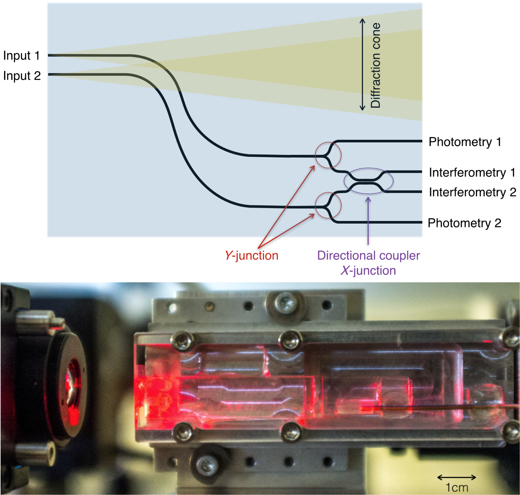
Figure 3. [Top] Illustration of the integrated optics nulling chip (not to scale). The input beams are fed into two inscribed waveguides. The waveguides undergo a smooth side step to avoid interference with the cone of uncoupled light. Two y-splitters form photometric monitors sampling the light in both beams. The waveguides are then routed to the directional coupler where the modes are mixed through evanescent coupling, producing the interference. [Bottom] Picture of the chip mounted in a metal bracket and back illuminated with a red laser.
GLINT South was designed, built, and tested at the 3.9-m AAT in Siding Spring Observatory, Australia. As the AAT does not have any facility AO system, GLINT South instrumentation is largely devoted to the injection of the light into the nulling chip. This is done with two active optics subsystems (Norris et al. Reference Norris2016) which can be seen in Figure 4. A tip and tilt mirror coupled to a detector in a closed loop provides the first-order correction of the atmospheric distortion, stabilising the seeing-limited beam on the instrument optical axis. Subsequently, the pupil of the telescope is imaged onto a segmented mirror capable of tip, tilt, and piston motion. Only two mirror segments are utilised to act as sub-apertures of our 2-beam interferometer. The outer-most segments are chosen to give GLINT the longest corresponding baseline of 2.7 m. The tip and tilt degrees of freedom are used to optimise for the injection into the chip, while the piston adjustment yields fine control of the baseline phase.
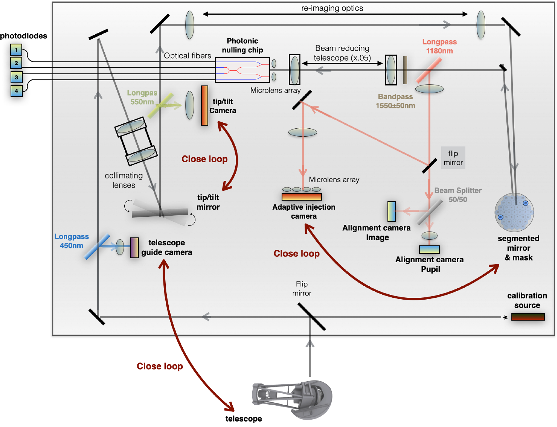
Figure 4. GLINT South schematic diagram. A flip mirror is used to easily switch between the light coming from the telescope and the light from the calibration source. The shortest wavelengths are reflected by a dichroic mirror onto the telescope guiding camera. A set of lenses collimate the light. A tip/tilt mirror works together with a camera in closed loop to maintain the beam on the optical axis against atmospheric seeing. A set of re-imaging optics relay the beam onto the segmented mirror where the pupil is re-imaged. A mask selects two sub-apertures for the 2-beam interferometer. The remaining visible light is sent to a camera where the sub-apertures are focused by a microlens array. The MEMS adaptive injection camera system works in closed loop to optimise the injection of the beams into the chip. The infrared beams transmitted by the last dichroic are concentrated by a factor of 20 and pass through a bandpass filter ( $\lambda = 1\,550 \pm 50$
nm). Finally, the beams are focused into the chip with a microlens array. The differential phase between the beams is controlled by pistoning the MEMS segment to add a path delay of
$\lambda = 1\,550 \pm 50$
nm). Finally, the beams are focused into the chip with a microlens array. The differential phase between the beams is controlled by pistoning the MEMS segment to add a path delay of $\frac{\pi}{2}$
, creating destructive inteference taking place inside the coupler of the chip. The resulting signals are carried out to photodiode detectors through single-mode fibres.
$\frac{\pi}{2}$
, creating destructive inteference taking place inside the coupler of the chip. The resulting signals are carried out to photodiode detectors through single-mode fibres.
2.1. Instrument layout
Figure 4 illustrates the layout of GLINT South. Custom lenses of focal lengths 112 and 300 mm have been designed to be achromatic from 600 to 1 600 nm, the visible light being used for the control systems, and the NIR for the nulling. The light is collected directly from the telescope’s M5 mirror (fifth reflection) where the beam has an F-number of 36. It hits a flip mirror that allows switching between the telescope and a calibration source fed from a fibre into a lens coupled with a diaphragm set to reproduce the F-number of the telescope. Different sources of illumination can be coupled through this same fibre for alignment, calibration, or measurement purposes. The shortest wavelengths are then reflected and focused onto the telescope guiding camera by a long-pass dichroic filter which has a cut-off of 450 nm.
The longer wavelength light passes through a pair of collimating lenses that re-image the telescope pupil onto the actuated tip/tilt mirror with steering precision of ${<}2\ \unicode[Times]{x03BC}$
rad and sensing speed of
${<}2\ \unicode[Times]{x03BC}$
rad and sensing speed of ${>}750$
Hz. The collimating system uses two of the 300-mm lenses to create an effective focal length of 163 mm resulting in an exit beam diameter of 4.2-mm matching the pupil to the micro-electro-mechanical systems (MEMS) mirror which comes downstream. The reflection off the tip/tilt mirror is split by the second dichroic filter with a 550-nm cut-off wavelength, where the ‘green’ components are focused onto a camera. The mirror and camera are operated in a close loop to correct for the two first-order aberrations from the atmosphere (tip and tilt) so that the beam undergoes minimal angular deviation with respect to the instrument optical axis.
${>}750$
Hz. The collimating system uses two of the 300-mm lenses to create an effective focal length of 163 mm resulting in an exit beam diameter of 4.2-mm matching the pupil to the micro-electro-mechanical systems (MEMS) mirror which comes downstream. The reflection off the tip/tilt mirror is split by the second dichroic filter with a 550-nm cut-off wavelength, where the ‘green’ components are focused onto a camera. The mirror and camera are operated in a close loop to correct for the two first-order aberrations from the atmosphere (tip and tilt) so that the beam undergoes minimal angular deviation with respect to the instrument optical axis.
The beam then goes through a 4-f system of relay optics, again using the custom made lenses, to re-image the pupil onto the segmented MEMS mirror while preserving the beam diameter. The MEMS is a core component of the GLINT instrument, each of the 37 segments ideally acts as a sub-aperture, with tip, tilt ( $\pm 4$
mrad), and piston(
$\pm 4$
mrad), and piston( $5\,\unicode[Times]{x03BC}$
m), allowing the modulation of the phase between the sub-apertures. A mask is placed right before the MEMS, approximately in the pupil plane to select the sub-apertures and reject stray light from adjacent segments.
$5\,\unicode[Times]{x03BC}$
m), allowing the modulation of the phase between the sub-apertures. A mask is placed right before the MEMS, approximately in the pupil plane to select the sub-apertures and reject stray light from adjacent segments.
In order to avoid distortion of the pupil on the MEMS, the light should hit the surface as nearly perpendicular as possible. A D-mirror (a circular mirror cut in half with a straight edge resembling the letter ‘D’) is used for this purpose to catch the reflection off the MEMS without blocking the incoming beam. The reflected light hits one last dichroic filter of 1 180-nm cut-off wavelength where the last visible light travels to a microlens array (MLA) focusing each sub-aperture onto a camera. The camera works in closed loop with the MEMS picking up the residual first- and second-order aberrations uncorrected by the tip and tilt mirror.
The remaining light transmitted through the last dichroic filter finally travels through a telescope, reducing the beam by a factor of 20. A bandpass filter of $\lambda = 1\,550 \pm 50$
nm matching the efficient bandpass of the nulling chip is placed in the collimated light. The beams from the individual sub-apertures are focused by another microlens array directly mounted on the chip, focusing each beam on its respective waveguide. Outputs of the nulling chip are carried through optical fibres into four independent photodiode detectors. An analogue to digital converter transforms the resulting voltage and transmits it to a computer. The signal from the detectors is acquired at a rate of 64 kilo-samples s–1. At this speed, the data are insensitive to the phase fluctuations within the individual exposures. The control systems are run on the same computer with a Matlab interface.
$\lambda = 1\,550 \pm 50$
nm matching the efficient bandpass of the nulling chip is placed in the collimated light. The beams from the individual sub-apertures are focused by another microlens array directly mounted on the chip, focusing each beam on its respective waveguide. Outputs of the nulling chip are carried through optical fibres into four independent photodiode detectors. An analogue to digital converter transforms the resulting voltage and transmits it to a computer. The signal from the detectors is acquired at a rate of 64 kilo-samples s–1. At this speed, the data are insensitive to the phase fluctuations within the individual exposures. The control systems are run on the same computer with a Matlab interface.
2.2. Alignment
A flip mirror is placed in the path of the adaptive injection camera to send the light to a pair of alignment cameras. The pupil is focused onto one of the cameras to align the mask to the segmented MEMS mirror. To align the nulling chip, a red laser is reverse injected through the output fibres of the chip, back-illuminating the set-up. The reflection off the shiny mask surface is observed with the pupil viewing camera. The chip is then translated along the optical axis within its micrometer precision 5-axis mount until the reflection is focused and translated horizontally and vertically to align it to the mask. The second camera focuses the image where classical fringes from the mask can be observed to check the alignment of the system.
To optimise the injection of the light into the chip, the segments of the MEMS perform a raster scan in tip and tilt providing a map of the throughput for each waveguide. This yields a mapping: the position on the adaptive injection camera corresponding to the maximum chip throughput is then tagged and used as the reference position for the control loop when on sky. Finally, a scan of the segments in piston is performed, resulting in the modulation of the interference intensity measured through the chip. The piston position corresponding to the maximum extinction is selected as a reference.
3. Null depth analysis
With GLINT, the interference between the sub-apertures occurs within the directional coupler of the nuller chip through evanescent coupling. A phase delay is applied to the beams by pistoning the segments of the MEMS mirror with respect to each other. The effective phase delay is a combination of the piston applied and the static phase delay within the chip. As a result, one of the directional coupler outputs carries the destructive interference ( $I_-$
), while the other carries the constructive interference (
$I_-$
), while the other carries the constructive interference ( $I_+$
). Additionally, the photometry of the incoming beams
$I_+$
). Additionally, the photometry of the incoming beams $I_1$
and
$I_1$
and $I_2$
are measured through the y-junctions. The extinction efficiency at any given time is determined by the instantaneous null depth defined as
$I_2$
are measured through the y-junctions. The extinction efficiency at any given time is determined by the instantaneous null depth defined as $N(t)=\frac{I_-(t)}{I_+(t)}$
.
$N(t)=\frac{I_-(t)}{I_+(t)}$
.
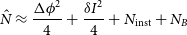
To fit and interpret the GLINT data, first a classical analysis of the interferometric signal is applied to derive an expression of the measured null depth $\hat{N}$
. Then a statistical model of the distribution of
$\hat{N}$
. Then a statistical model of the distribution of $\hat{N}$
is derived. This follows the null self-calibration approach of Hanot et al. (Reference Hanot2011) with adjustments for GLINT (also used in GLINT North (Norris et al. Reference Norris2020; Martinod et al. Reference Martinod2021a)). This statistical approach allowed Hanot et al. to fit nulled data with higher accuracy than conventional analysis as well as removed the need for a stellar calibration of the null depth.
$\hat{N}$
is derived. This follows the null self-calibration approach of Hanot et al. (Reference Hanot2011) with adjustments for GLINT (also used in GLINT North (Norris et al. Reference Norris2020; Martinod et al. Reference Martinod2021a)). This statistical approach allowed Hanot et al. to fit nulled data with higher accuracy than conventional analysis as well as removed the need for a stellar calibration of the null depth.
3.1. Analytical expression of the measured null depth $\hat{\boldsymbol{N}}$

For a monochromatic point source in a perfect interferometer, the coherent superposition of two beams of intensity $I_1$
and
$I_1$
and $I_2$
produces an interference whose intensity I depends on the phase difference
$I_2$
produces an interference whose intensity I depends on the phase difference $\Delta \phi$
between the beams
$\Delta \phi$
between the beams $\Delta \phi = \phi_1 - \phi_2 = \frac{2\pi\Delta x}{\lambda}$
, where
$\Delta \phi = \phi_1 - \phi_2 = \frac{2\pi\Delta x}{\lambda}$
, where $\Delta x$
is the pathlength difference and
$\Delta x$
is the pathlength difference and $\lambda$
the wavelength:
$\lambda$
the wavelength:
 \begin{equation} I = \frac{1}{2} \left[ I_1 + I_2 + 2\sqrt{I_1I_2}\cos (\Delta \phi) \right]. \end{equation}
I is maximum ( $I_+$
) when
$I_+$
) when $\Delta \phi$
is a multiple of
$\Delta \phi$
is a multiple of $ 2 \pi $
and minimum (
$ 2 \pi $
and minimum ( $I_-$
) when an integer multiple of
$I_-$
) when an integer multiple of $\pi$
. When the null depth is only limited by a small beam imbalance
$\pi$
. When the null depth is only limited by a small beam imbalance $\delta I = \frac{I_1 - I_2}{I_1+I_2}$
and a small pathlength error (
$\delta I = \frac{I_1 - I_2}{I_1+I_2}$
and a small pathlength error ( $\Delta \phi \approx 0$
), the instantaneous null depth can be approximated by:
$\Delta \phi \approx 0$
), the instantaneous null depth can be approximated by:
 \begin{equation} N \approx \frac{\Delta \phi^2}{4} + \frac{\delta I^2}{4}\end{equation}
(Serabyn Reference Serabyn, Léna and Quirrenbach2000; Hanot et al. Reference Hanot2011). For an extended source (e.g. a resolved star, protoplanetary disc, star with a companion), the resolved light originating at an angular distance of $\theta$
off-axis undergoes an additional path delay
$\theta$
off-axis undergoes an additional path delay $B \sin(\theta)$
(with B the baseline). This does not interfere coherently with the ‘on-axis’ starlight, resulting in the superposition of the interference as illustrated in Figure 1 for the case of an unresolved star with a planet. This additional contribution is denoted as the astronomical null depth
$B \sin(\theta)$
(with B the baseline). This does not interfere coherently with the ‘on-axis’ starlight, resulting in the superposition of the interference as illustrated in Figure 1 for the case of an unresolved star with a planet. This additional contribution is denoted as the astronomical null depth $N_a$
which is the quantity of interest in nulling interferometry. Measuring
$N_a$
which is the quantity of interest in nulling interferometry. Measuring $N_a$
on different baselines B provides a spatial coherence map, to which astronomical models can be fitted to describe the geometric profile of the region surrounding the source, revealed by the attenuation of the star. In order to use this technique for exoplanet detection and characterisation, deep null depths (high attenuation with minimal photon noise) and precisely calibrated astronomical null depths (for the ability to detect a companion signal at contrast ratio deeper than the mean instrumental null depth) are necessary.
$N_a$
on different baselines B provides a spatial coherence map, to which astronomical models can be fitted to describe the geometric profile of the region surrounding the source, revealed by the attenuation of the star. In order to use this technique for exoplanet detection and characterisation, deep null depths (high attenuation with minimal photon noise) and precisely calibrated astronomical null depths (for the ability to detect a companion signal at contrast ratio deeper than the mean instrumental null depth) are necessary.
In practice, a background term $I_B$
adds to the measured null depth
$I_B$
adds to the measured null depth $\hat{N}$
as well as an instrumental leakage term
$\hat{N}$
as well as an instrumental leakage term $N_{\rm inst}$
corresponding to instrumental errors including the chromatic error and polarisation mismatch. The instrument leakage must be characterised so that it can be subtracted as a bias from the astronomical data:
$N_{\rm inst}$
corresponding to instrumental errors including the chromatic error and polarisation mismatch. The instrument leakage must be characterised so that it can be subtracted as a bias from the astronomical data:
 \begin{equation}\hat{N} = \frac{I_- + I_{B-}}{I_+ + I_{B+}} + N_{\rm inst} + N_a. \end{equation}
For laboratory measurements, the flux in $I_+$
is typically larger than the background, so it is approximated that mostly the background in the null
$I_+$
is typically larger than the background, so it is approximated that mostly the background in the null $I_-$
contributes significantly to a degradation of the null depth. Furthermore,
$I_-$
contributes significantly to a degradation of the null depth. Furthermore, $N_a=0$
for a laboratory spatially coherent source. Hence, the modelled
$N_a=0$
for a laboratory spatially coherent source. Hence, the modelled $\hat{N}$
for GLINT simplifies to
$\hat{N}$
for GLINT simplifies to
 \begin{equation} \hat{N} \approx \frac{\Delta \phi^2}{4} + \frac{\delta I^2}{4} + N_{\rm inst} + N_B \end{equation}
using $N_B = \frac{I_{B-}}{I_+}$
.
$N_B = \frac{I_{B-}}{I_+}$
.
3.2. Statistical distribution of the measured null depth
$\hat{N}$

To fit the nulled data, Hanot et al. (Reference Hanot2011) looked at the statistical distribution of $\hat{N}$
which alleviates the need for perfect fringe tracking as well as yielding higher accuracy of the fitted data. This also allows using longer integration times, improving the signal-to-noise ratio. To derive the model,
$\hat{N}$
which alleviates the need for perfect fringe tracking as well as yielding higher accuracy of the fitted data. This also allows using longer integration times, improving the signal-to-noise ratio. To derive the model, $\Delta \phi$
,
$\Delta \phi$
, $\delta I$
, and
$\delta I$
, and $N_B$
are assumed to follow normal distributions.
$N_B$
are assumed to follow normal distributions. $\Delta\phi$
is not measured and left as a free parameter for the fitting. The probability distribution function (PDF) of a normal variable X is given by:
$\Delta\phi$
is not measured and left as a free parameter for the fitting. The probability distribution function (PDF) of a normal variable X is given by:
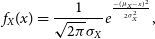 \begin{equation}f_{X}(x) = \frac{1}{\sqrt{2\pi}\sigma_X} e^{\frac{-(\mu_X - x)^2}{2\sigma_X^2}},\end{equation}
with $\mu_X$
is the mean and
$\mu_X$
is the mean and $\sigma_X$
is the standard deviation of the variable X.
$\sigma_X$
is the standard deviation of the variable X.
To compute the distribution of $\Delta\phi^2$
and
$\Delta\phi^2$
and $\delta I^2$
, a change of variable
$\delta I^2$
, a change of variable $X \rightarrow Y = \frac{X^2}{4}$
is applied to Equation (5) giving
$X \rightarrow Y = \frac{X^2}{4}$
is applied to Equation (5) giving
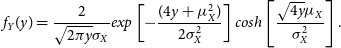 \begin{equation} f_Y(y) = \frac{2}{\sqrt{2\pi y}\sigma_X}exp\left[ - \frac{(4y+\mu_X^2)}{2\sigma_X^2}\right] cosh\left[\frac{\sqrt{4y}\mu_X}{\sigma_X^2}\right]. \end{equation}
The final distribution of $\hat{N}$
is obtained by convolving the distributions
$\hat{N}$
is obtained by convolving the distributions $PDF(\frac{\Delta\phi^2}{4})$
,
$PDF(\frac{\Delta\phi^2}{4})$
, $PDF(\frac{\delta I^2}{4})$
,
$PDF(\frac{\delta I^2}{4})$
, $PDF({N_B})$
, and
$PDF({N_B})$
, and $N_{\rm inst}$
. With GLINT,
$N_{\rm inst}$
. With GLINT, $\delta I$
and
$\delta I$
and $N_B$
are directly measured, their convolutions are calculated numerically and the three parameters
$N_B$
are directly measured, their convolutions are calculated numerically and the three parameters $\mu(\Delta\phi)$
,
$\mu(\Delta\phi)$
, $\sigma(\Delta\phi)$
, and
$\sigma(\Delta\phi)$
, and $N_{\rm inst}$
are fitted with a least square minimum algorithm, similar to the null self-calibrated method in Mennesson et al. (Reference Mennesson, Malbet, Creech-Eakman and Tuthill2016). Figure 5 shows the construction of the measured null depth distribution with the statistical distributions of the different terms. This works well under laboratory conditions where the phase and intensity fluctuations are small, drawing normal distributions as assumed by the analytical model. For on-sky data, this assumption is no longer valid; instead a Monte Carlo approach is used to generate the fluctuations (discarding the assumption of normally distributed data) which is detailed in Norris et al. (Reference Norris2020). Obtaining a best fit to the data by way of this latter method is more time-consuming but produces more accurate fits. Investigation of the model fitting with simulated data showed that data can be fitted with a precision of
$N_{\rm inst}$
are fitted with a least square minimum algorithm, similar to the null self-calibrated method in Mennesson et al. (Reference Mennesson, Malbet, Creech-Eakman and Tuthill2016). Figure 5 shows the construction of the measured null depth distribution with the statistical distributions of the different terms. This works well under laboratory conditions where the phase and intensity fluctuations are small, drawing normal distributions as assumed by the analytical model. For on-sky data, this assumption is no longer valid; instead a Monte Carlo approach is used to generate the fluctuations (discarding the assumption of normally distributed data) which is detailed in Norris et al. (Reference Norris2020). Obtaining a best fit to the data by way of this latter method is more time-consuming but produces more accurate fits. Investigation of the model fitting with simulated data showed that data can be fitted with a precision of $10^{-3}$
which is used as error bars for all null depths estimated with this method.
$10^{-3}$
which is used as error bars for all null depths estimated with this method.
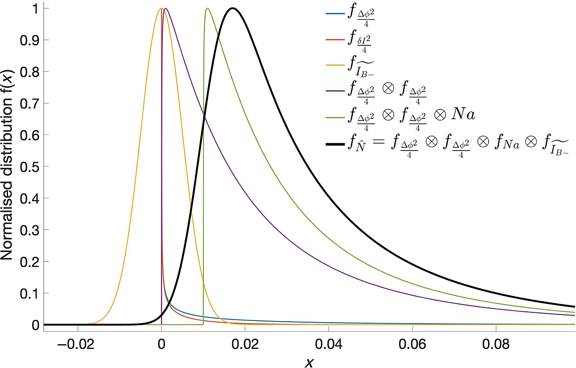
Figure 5. Illustration of the different statistical distributions involved in the construction of the analytical model to fit the null data. The symbols identifying the different linetypes follow the nomenclature from the text.
4. Laboratory characterisation
In order to calibrate the null data, GLINT was first characterised experimentally in a controlled environment laboratory (temperature was stabilised at $18^{\circ}\, \pm\, 0.1^{\circ}\,\text{C}$
with 0% humidity). This ensured instrumental stability and repeatability of measurements.
$18^{\circ}\, \pm\, 0.1^{\circ}\,\text{C}$
with 0% humidity). This ensured instrumental stability and repeatability of measurements.
4.1. Splitting ratios
The splitting ratios between the photometric taps and the coupler of the chip were measured experimentally in order to scale the intensities $I_1$
and
$I_1$
and $I_2$
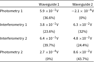
in Equation (1). These splitting ratios are largely an intrinsic property of the geometry of the waveguide fabrication around the location of the Y-junction, and although they were designed to be 1/3, they can vary due to small unpredictable variations in the manufacturing process. These ratios are wavelength-dependent. Here, a superluminescent diode light source (centred at 1 550 nm) was injected into each individual waveguide and the resulting throughput was measured at the output of the chip. The time-averaged intensities measured are recorded in Table 1.
$I_2$
in Equation (1). These splitting ratios are largely an intrinsic property of the geometry of the waveguide fabrication around the location of the Y-junction, and although they were designed to be 1/3, they can vary due to small unpredictable variations in the manufacturing process. These ratios are wavelength-dependent. Here, a superluminescent diode light source (centred at 1 550 nm) was injected into each individual waveguide and the resulting throughput was measured at the output of the chip. The time-averaged intensities measured are recorded in Table 1.
Table 1. Averaged raw voltages (bias subtracted) measured in the four outputs of the nulling chip for illuminating input 1 and 2 independently and the corresponding percentage of the signal injected in the chip. The non-null measurements observed in the photometric channels when they are not illuminated come from the measurement error of the order $10^{-4}$
.
$10^{-4}$
.
Ignoring all the chip’s intrinsic losses, the splitting ratio A for the photometric channel 1 is the ratio of the intensity measured in channel 1 over the intensity injected in waveguide 1:
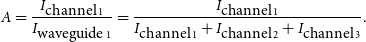 \begin{equation} A = \frac{I_{\mbox{channel}\,1}}{I_{\mbox{waveguide}\,1}} = \frac{I_{\mbox{channel}\, 1}}{I_{\mbox{channel}\,1}+I_{\mbox{channel}\,2} + I_{\mbox{channel}\,3}}.\end{equation}
channels 2 and 3 represent the two outputs of the couplers (normally the output carrying the interferometric null and anti-null). Hence, if $I_{\mbox{channel}\,1}$
is monitoring the photometry, then intensity
$I_{\mbox{channel}\,1}$
is monitoring the photometry, then intensity $I_1$
into the coupler is
$I_1$
into the coupler is
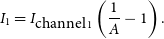 \begin{equation} I_1 = I_{\mbox{channel}\,1} \left( \frac{1}{A} - 1 \right).\end{equation}
Similarly, if B is the splitting coefficient of the y-splitter of waveguide 2, and the intensity in channel 4 measures the photometry then:
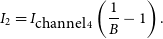 \begin{equation} I_2 = I_{\mbox{channel}\,4} \left( \frac{1}{B} - 1 \right).\end{equation}
From Table 1, it is found that $A=0.37$
and
$A=0.37$
and $B = 0.43$
, which exhibit some deviation from the intended 0.33. In this experiment, only one field is injected at a time, hence there is no coherent superposition in the x-junction so that the intensities in the interferometric channels are not balanced. It should also be noted that the raw intensities from waveguide 2 are significantly lower than from waveguide 1. This was observed consistently through all measurements performed with GLINT South. It is suspected that a misalignment of the GLINT South MLA with respect to the chip preferentially degrades the coupling into waveguide 2.
$B = 0.43$
, which exhibit some deviation from the intended 0.33. In this experiment, only one field is injected at a time, hence there is no coherent superposition in the x-junction so that the intensities in the interferometric channels are not balanced. It should also be noted that the raw intensities from waveguide 2 are significantly lower than from waveguide 1. This was observed consistently through all measurements performed with GLINT South. It is suspected that a misalignment of the GLINT South MLA with respect to the chip preferentially degrades the coupling into waveguide 2.
4.2. Characterisation of the null depth’s chromaticity
One limitation of the statistical model is that it assumes a perfectly monochromatic source. In reality, the nulling chip is presented with some spectral bandpass, over which the coupling is chromatic. This is due in part to the fact that the substrate of the chip is a dispersive material, and even more to the physics of evanescent coupling (which is determined by the length of the x-coupler and the wavelength) (Okamoto Reference Okamoto2006). This contributes to the degradation of the null depth. To investigate this effect, the instrumental null depth ( $N_{\rm inst}$
) as a function of wavelength was measured through GLINT South. For this experiment, the bandpass filter (
$N_{\rm inst}$
) as a function of wavelength was measured through GLINT South. For this experiment, the bandpass filter ( $\lambda$
= 1 550 nm,
$\lambda$
= 1 550 nm, $\Delta \lambda$
= 50 nm) was removed. A tunable laser was used together with a wavemeter to accurately calibrate the wavelength. The null depth was measured for wavelengths between 1 511.4 and 1 628.7 nm in steps of 10 nm. The null depth was fitted to the data using the analytical form of the statistical model for each wavelength and is plotted in Figure 6, with data tabulated on the side, with error bars of
$\Delta \lambda$
= 50 nm) was removed. A tunable laser was used together with a wavemeter to accurately calibrate the wavelength. The null depth was measured for wavelengths between 1 511.4 and 1 628.7 nm in steps of 10 nm. The null depth was fitted to the data using the analytical form of the statistical model for each wavelength and is plotted in Figure 6, with data tabulated on the side, with error bars of $10^{-3}$
as defined by the fitting accuracy of the model.
$10^{-3}$
as defined by the fitting accuracy of the model.
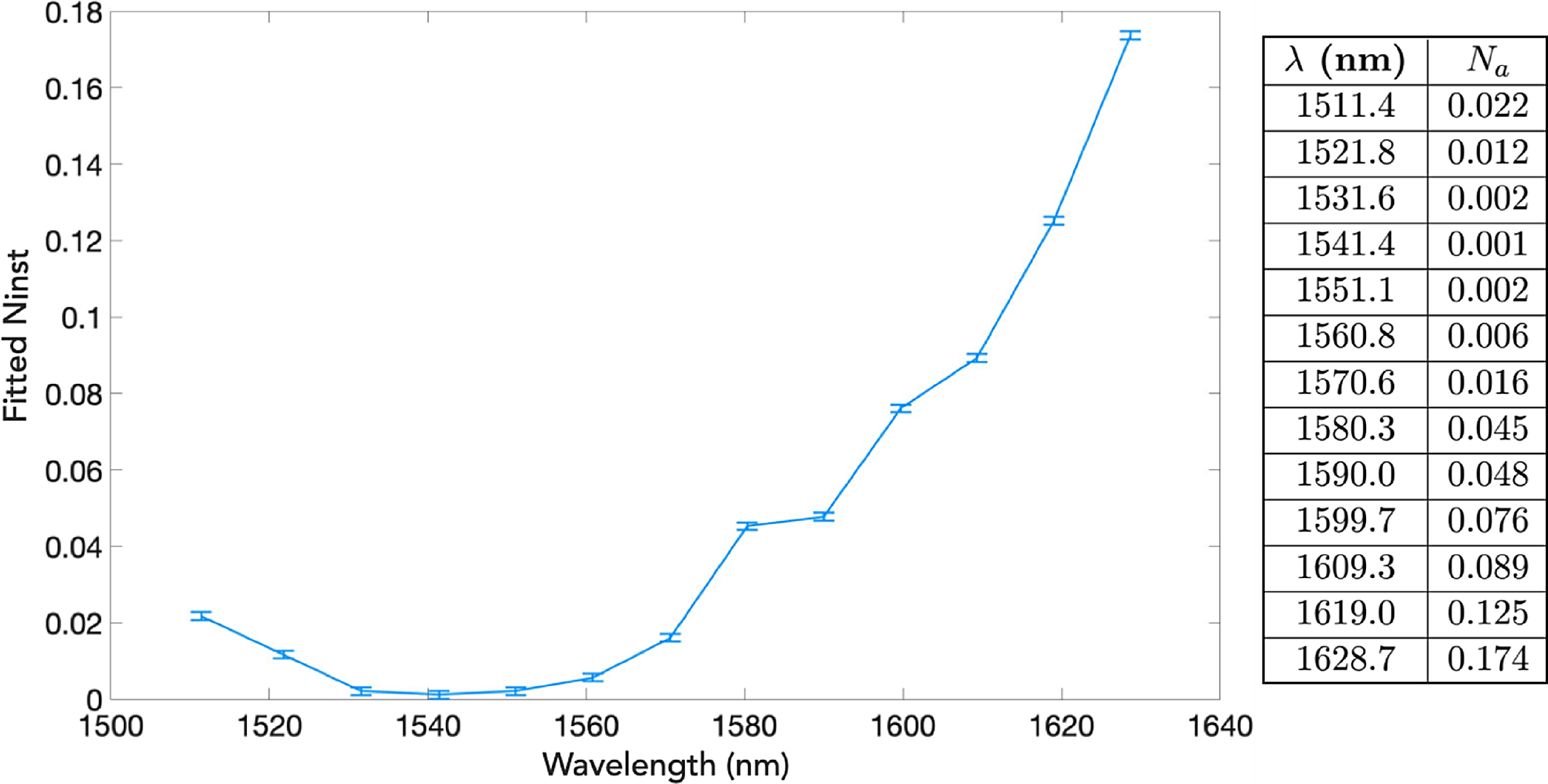
Figure 6. Fitted null depth as a function of wavelength. Data are tabulated to the right.
It was found that the best null depth was obtained at 1 541.4 nm (slightly off the theoretical value of 1 550 nm targeted during fabrication) with a fitted null depth of $0.001 \pm 0.001$
. It can be deduced that with the precision of 0.001 on the null depth measured, the monochromatic null depth is close to zero. To put it another way, the measured null leakage is dominated by chromatic effects. To quantify the chromatic contribution to the measured null depth, values from Figure 6 between the instrumental bandpass
$0.001 \pm 0.001$
. It can be deduced that with the precision of 0.001 on the null depth measured, the monochromatic null depth is close to zero. To put it another way, the measured null leakage is dominated by chromatic effects. To quantify the chromatic contribution to the measured null depth, values from Figure 6 between the instrumental bandpass $\Delta\lambda =[1\,525, 1\,575]$
nm were interpolated and averaged to 0.006. Substracting the minimum null depth of 0.001, the chromatic contribution to the null depth is estimated to 0.005.
$\Delta\lambda =[1\,525, 1\,575]$
nm were interpolated and averaged to 0.006. Substracting the minimum null depth of 0.001, the chromatic contribution to the null depth is estimated to 0.005.
For the long-term goal of performing high-contrast nulling of starlight to image exoplanets, the ability to achieve a broadband deep null is crucial. Employing a wider bandpass significantly increases the photon flux available hence the signal to noise ratio, which is important in the faint-signal use case when targeting exoplanets.
5. On-sky results
GLINT South was interfaced and tested on the 3.9–m AAT in Siding Spring for a total of 16 nights in July, November 2016 and June, July, August 2017 in order to test the control systems and demonstrate the on-sky nulling capability.
5.1. Starlight injection
The first observing campaign was utilised to characterise the telescope seeing-limited point spread function (PSF) and constrain the stroke and speed requirements for the two control systems to inject starlight efficiently in the chip. Subsequently, the control systems were tested in November 2016 on the bright star $\alpha$
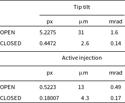
Scorpii. The position of the PSF as a function of time was recorded for the tip/tilt (TT) and adaptive injection (AI) systems with the loop open and closed. The results are shown in Figures 7, 8 and summarised in Table 2. It can be seen that the two loops performed well, reducing the pointing jitter from the turbulent atmosphere by a factor of
$\alpha$
Scorpii. The position of the PSF as a function of time was recorded for the tip/tilt (TT) and adaptive injection (AI) systems with the loop open and closed. The results are shown in Figures 7, 8 and summarised in Table 2. It can be seen that the two loops performed well, reducing the pointing jitter from the turbulent atmosphere by a factor of ${\approx}11$
for the TT system and another factor of
${\approx}11$
for the TT system and another factor of ${\approx}3$
for the AI system.
${\approx}3$
for the AI system.
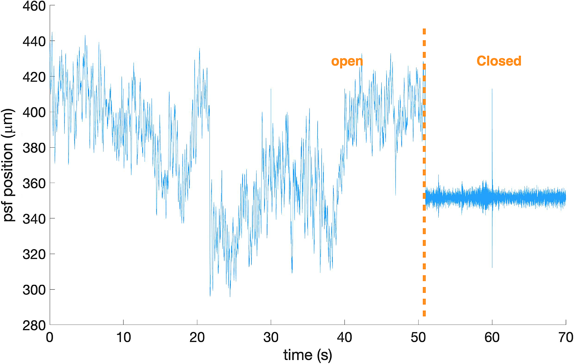
Figure 7. PSF position (converted to a vector length from the x and y centroid position) on the TT camera as a function of time with the TT loop open (left) and closed (right). The zero point (for closing the loop) was defined by the position of the PSF on the camera with the calibration source. Data recorded for the star $\alpha$
Scorpii on the 2017 June 6 at 03:07am with a seeing of 1".
$\alpha$
Scorpii on the 2017 June 6 at 03:07am with a seeing of 1".
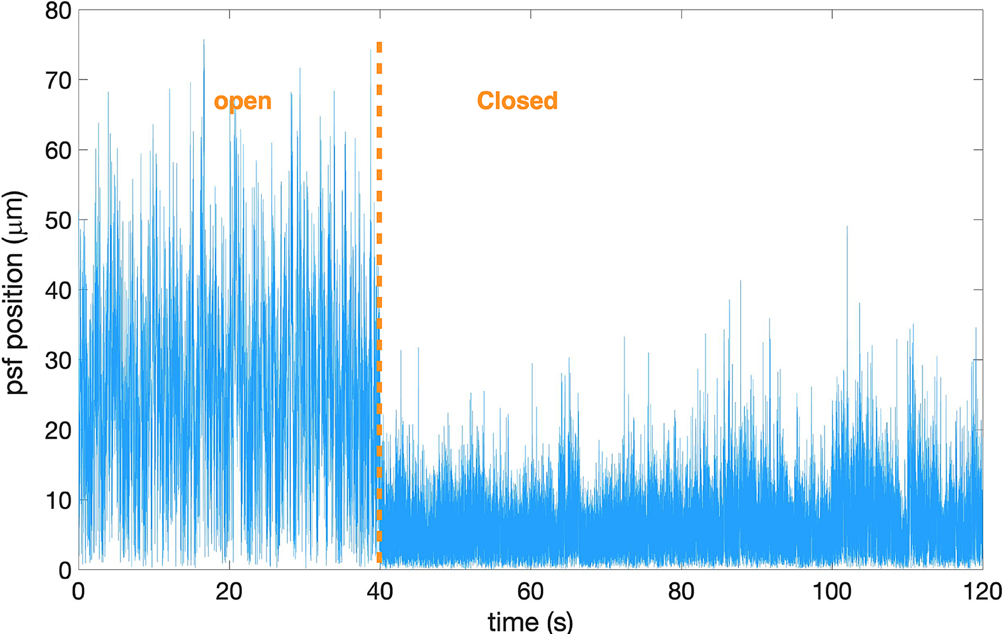
Figure 8. PSF position on the AI camera as a function of time with the AI loop open and closed (TT closed). The zero point (for closing the loop) was defined by the position of the PSF on the camera with the calibration source. Data recorded for the star $\alpha$
Scorpii on the 2017 June 6 at 03:07am with a seeing of 1".
$\alpha$
Scorpii on the 2017 June 6 at 03:07am with a seeing of 1".
Table 2. Averaged standard deviation of the PSF converted to tip/tilt angle errors for the TT (top) and AI (bottom) loop open and closed.
5.2. Measuring angular diameters of bright Mira stars
A sample of infrared-bright stars was selected for observation. In addition to practical considerations such as observability and sufficient predicted count rates, stars were chosen also for the ability of the instrument to deliver a scientific outcome: an astrophysical contribution to the null depth. Therefore, stars with relatively large apparent angular diameters (although still somewhat below the formal diffraction limit of the 3.9 m AAT) were preferred. Accordingly, no unresolved stars were observed, which would have provided a stronger null capability demonstration of GLINT South. For each star, approximately 1 hour of data was acquired.
Data were reduced and analysed using the Monte Carlo statistical model. Subsequently a diameter was calculated for each star using the null depth versus stellar diameter relationship from Absil et al. (Reference Absil, den Hartog, Gondoin, Fabry, Wilhelm, Gitton and Puech2011, Reference Absil, den Hartog, Gondoin, Fabry, Wilhelm, Gitton and Puech2006). Given the small baseline considered, we ignored the effect of limb darkening and assumed stars with uniform discs. The characterised chromatic instrumental contribution to the null depth is subtracted from the on-sky measured null depth. The error bars on the astronomical null depth are estimated to be $1 \times 10^{-3}$
(from the precision imposed by the model fitting of the data) which corresponds to 5 mas. The results are summarised and compared to literature values in Table 3. To assess the quality of the fitted data, the average of the raw detector voltages measured in the first photometric channel is given in the third column. When the voltage is less than
$1 \times 10^{-3}$
(from the precision imposed by the model fitting of the data) which corresponds to 5 mas. The results are summarised and compared to literature values in Table 3. To assess the quality of the fitted data, the average of the raw detector voltages measured in the first photometric channel is given in the third column. When the voltage is less than ${\sim}10^{-2}$
V, the null depth distribution is dominated by the dark current. To illustrate this, the null depth distribution of
${\sim}10^{-2}$
V, the null depth distribution is dominated by the dark current. To illustrate this, the null depth distribution of $\alpha$
Scorpii and Alpha Tauri are shown in Figures 9 and 10, respectively.
$\alpha$
Scorpii and Alpha Tauri are shown in Figures 9 and 10, respectively. $\alpha$
Scorpii displayed good signal-to-noise ratio and illustrates the expected asymmetric statistical distribution. On the other hand, the statistical distribution of
$\alpha$
Scorpii displayed good signal-to-noise ratio and illustrates the expected asymmetric statistical distribution. On the other hand, the statistical distribution of $\alpha$
Tauri data exhibited poor signal-to-noise ratio dominated by the symmetric Gaussian dark noise. As a result, the fitted null depth is poorly constrained and it was not possible to extrapolate an accurate stellar diameter.
$\alpha$
Tauri data exhibited poor signal-to-noise ratio dominated by the symmetric Gaussian dark noise. As a result, the fitted null depth is poorly constrained and it was not possible to extrapolate an accurate stellar diameter.
It is noteworthy that all stellar diameters recovered in Table 3 are formally unresolved: that is they are smaller than the diffraction limit of the telescope at these wavelengths ( ${\approx}100$
mas). These results were also obtained at >1 arcsec seeing with no AO system. Furthermore, GLINT has yielded accurate measurements without the usual interferometric practice of calibrating the system transfer function by way of separate observations of an unresolved stellar point source reference. For the high signal-to-noise data, the fitted diameters match those of the literature to within 1
${\approx}100$
mas). These results were also obtained at >1 arcsec seeing with no AO system. Furthermore, GLINT has yielded accurate measurements without the usual interferometric practice of calibrating the system transfer function by way of separate observations of an unresolved stellar point source reference. For the high signal-to-noise data, the fitted diameters match those of the literature to within 1 $\sigma$
, the difference being a tiny fraction of the diffraction limit. From an astrophysical standpoint, perfect correspondence to the literature sizes is not to be expected as red giant/supergiant stars are generally strongly variable both in time (with pulsations) and with wavelength (due to their complex molecular atmospheres). We conclude that the primary instrumental limitation for GLINT South is the poor sensitivity of the photodiode detectors used.
$\sigma$
, the difference being a tiny fraction of the diffraction limit. From an astrophysical standpoint, perfect correspondence to the literature sizes is not to be expected as red giant/supergiant stars are generally strongly variable both in time (with pulsations) and with wavelength (due to their complex molecular atmospheres). We conclude that the primary instrumental limitation for GLINT South is the poor sensitivity of the photodiode detectors used.
We now proceed with a very brief discussion of results, touching on individual stars.
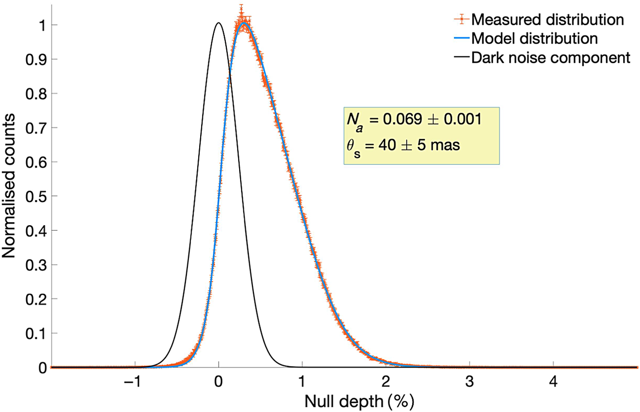
Figure 9. Null depth distribution over plotted with the dark noise for the star $\alpha$
Scorpii, with the measured astrophysical null (
$\alpha$
Scorpii, with the measured astrophysical null ( $N_a$
) and corresponding uniform disc diameter (
$N_a$
) and corresponding uniform disc diameter ( $\theta_s$
) indicated. This is close to the literature diameter of 41.30 mas (Richichi, Percheron, & Khristoforova Reference Richichi, Percheron and Khristoforova2005).
$\theta_s$
) indicated. This is close to the literature diameter of 41.30 mas (Richichi, Percheron, & Khristoforova Reference Richichi, Percheron and Khristoforova2005).
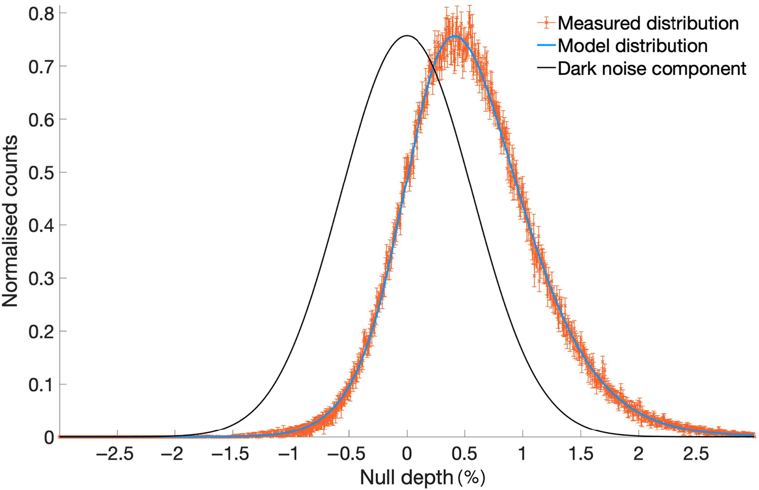
Figure 10. Null depth distribution over plotted with the dark noise for the star $\alpha$
Tauri. The distribution is dominated by the dark noise which can be seen by the Gaussian shape of the curve. An accurate
$\alpha$
Tauri. The distribution is dominated by the dark noise which can be seen by the Gaussian shape of the curve. An accurate $N_a$
could not be determined.
$N_a$
could not be determined. $\alpha$
Scorpii (Figure 9) is a red supergiant and one of the few stars that has had its surface imaged showing a complex atmosphere with variable dark spots (Ohnaka, Weigelt, & Hofmann Reference Ohnaka, Weigelt and Hofmann2017). Its data were acquired with a seeing of 1.1" measured at the AAT. Its measured angular diameter of
$\alpha$
Scorpii (Figure 9) is a red supergiant and one of the few stars that has had its surface imaged showing a complex atmosphere with variable dark spots (Ohnaka, Weigelt, & Hofmann Reference Ohnaka, Weigelt and Hofmann2017). Its data were acquired with a seeing of 1.1" measured at the AAT. Its measured angular diameter of $40 \pm 5$
mas with GLINT matches well with values reported in the literature.
$40 \pm 5$
mas with GLINT matches well with values reported in the literature.
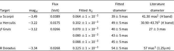
Table 3. Fitted $N_a$
, with corresponding fitted diameter using a uniform disk model, compared to the literature diameter.
$N_a$
, with corresponding fitted diameter using a uniform disk model, compared to the literature diameter. $\mathrm{mag}_H$
gives the magnitude of the star in the H band and flux, the averaged flux measured by GLINT (in the first photometric channel).
$\mathrm{mag}_H$
gives the magnitude of the star in the H band and flux, the averaged flux measured by GLINT (in the first photometric channel). $\alpha$
Herculis fitted diameter differs from the litterature value; however, they cannot be compared fairly as the values are for different spectral bands. For all other stars, the fitted stellar diameters agree with literature values.
$\alpha$
Herculis fitted diameter differs from the litterature value; however, they cannot be compared fairly as the values are for different spectral bands. For all other stars, the fitted stellar diameters agree with literature values.
 $\alpha$
Herculis is a luminous red bright giant with a companion separated by more than 3.3 arcsec. Although no literature diameter values could be found in the H band, K band angular diameters reported in the literature vary by up to 30%, possibly partly a consequence of its variable nature. The recorded seeing for this star was 1" and measured diameter
$\alpha$
Herculis is a luminous red bright giant with a companion separated by more than 3.3 arcsec. Although no literature diameter values could be found in the H band, K band angular diameters reported in the literature vary by up to 30%, possibly partly a consequence of its variable nature. The recorded seeing for this star was 1" and measured diameter $49 \pm 5\,\mathrm{mas}$
, within the bounds of the literature values.
$49 \pm 5\,\mathrm{mas}$
, within the bounds of the literature values. $\beta$
Gruis is a variable red giant star. Three sequential data sets were acquired on
$\beta$
Gruis is a variable red giant star. Three sequential data sets were acquired on $\beta$
Gruis in seeing of 1.1". The astronomical null depth fitted shows a small increase over the measurements which could be accounted for by small drift in the instrument as the optimisation steps were only performed prior to the first measurement. The angular diameters fit to 41, 42, and
$\beta$
Gruis in seeing of 1.1". The astronomical null depth fitted shows a small increase over the measurements which could be accounted for by small drift in the instrument as the optimisation steps were only performed prior to the first measurement. The angular diameters fit to 41, 42, and $44 \pm 5\,\mathrm{mas}$
.
$44 \pm 5\,\mathrm{mas}$
. $\beta$
Gruis has previously been resolved at 600 nm at the AAT with an angular diameter of
$\beta$
Gruis has previously been resolved at 600 nm at the AAT with an angular diameter of $27 \pm 3\,\mathrm{mas}$
(Bedding, Robertson, & Marson Reference Bedding, Robertson and Marson1994), but no data were found for the near infrared.
$27 \pm 3\,\mathrm{mas}$
(Bedding, Robertson, & Marson Reference Bedding, Robertson and Marson1994), but no data were found for the near infrared.
R Doradus is also a long-period variable red giant star with an angular diameter of 57 mas measured at 1.25 $\unicode[Times]{x03BC}$
m (Richichi et al. Reference Richichi, Percheron and Khristoforova2005), making it one of the largest stars in apparent diameter. GLINT obtained an angular diameter of
$\unicode[Times]{x03BC}$
m (Richichi et al. Reference Richichi, Percheron and Khristoforova2005), making it one of the largest stars in apparent diameter. GLINT obtained an angular diameter of $54 \pm 5\,\mathrm{mas}$
which is
$54 \pm 5\,\mathrm{mas}$
which is ${\approx}5\,\%$
away from (and within errors of) the literature value.
${\approx}5\,\%$
away from (and within errors of) the literature value.
6. Conclusion
Nulling interferometry has been identified as one of the most promising techniques to tackle the challenges of Earth-like exoplanet characterisation. Predecessor projects such as the PFN have paved the way achieving null depths as low as a few $10^{-4}$
.
$10^{-4}$
.
The GLINT programme is an ongoing instrumental effort to further advance the technique by utilising novel photonic technology: the nulling of the starlight is produced with high coherence and stability inside an integrated optic. The direct-write method is exploited for its robustness, short lead times, flexibility, and scalability of designs through three-dimensional geometry. Ideally, a photonic chip can be designed to remap an entire telescope pupil into different nulling baselines, increasing the signal to noise ratio as well as the spatial information retrieved from the observed source. GLINT South was designed as a testbed for such devices at the AAT with a unique active optics system compensating the first-order atmospheric distortions and optimising the delicate starlight injection into the photonic chip. The instrument was tested on-sky, performing the stabilisation of the injection which further allowed the observation of four evolved cool giant stars. Using a modified statistical model to fit and interpret the data, angular diameters below the diffraction limit of the telescope and in close agreement to the literature were obtained validating and demonstrating the potential of the instrumental concept.
This paper has demonstrated the successful commissioning of GLINT South, a testbed to prototype technologies for nulling interferometry. The seeing-limited telescope limits the science at such a site, but this testbed can be used to pioneer new approaches on-sky, that can then be directly injected into GLINT North at the scientifically competitive Subaru Telescope which is equipped of a high performance AO system. With on-sky time on large telescopes being hard to access, this development model will allow for much more rapid improvements of nulling interferometry.
In order to reach the goal of direct exoplanetary observations, null depths still need to be improved by a few orders of magnitude. GLINT characterisation found that the instrument sensitivity is limited by dark noise and chromaticity. This can be addressed by injecting a larger area of telescope pupil, using a more sensitive detector, recovering more baselines and a system to implement dispersion of the fringe (Martinod et al. Reference Martinod2021a). On the other hand, the null depth is affected by errors in the wavefronts and in the injection. Future and more stable mounts and structure may help, for example, the incorporation of more optical processes into the photonic chip. However, the most significant improvements are delivered with more powerful AO systems. Similarly, a fringe tracker brings significant improvements to the null depth (Martin et al. Reference Martin, Heidmann, Rauch, Jocou and Courjal2014), which can also be built into the photonic chip through a tricoupler architecture (Martinod et al. Reference Martinod, Tuthill, Gross, Norris, Sweeney and Withford2021b). These techniques of active corrections and tracking can be combined to reach null depths deeper than with any technique individually.
The importance of the careful characterisation of the photonic device was highlighted in this work and will be even more critical in the future, as more complex geometries are implemented. Recent advances to GLINT at the Subaru Telescope, include implementing a more advanced chip with six effective baselines all spectrally dispersed on a more sensitive detector (Martinod et al. Reference Martinod2021a). In parallel, asymmetric couplers are being investigated for achromatic coupling (Chen et al. Reference Chen, Eaton, Zhang and Herman2008). Furthermore, the direct-write technique is currently limited to the telecommunication band of 1 550 nm, a region where scientific inquiries of exoplanets are somewhat more challenging due to the higher contrast required by reflected light observations. Mid-IR regions at longer wavelength are better suited due to more favourable contrast ratios between the star and planet ( $10^{-6}/10^{-7}$
), as well as encompassing interesting geo- and bio-signatures. Efforts are also being undertaken to push the direct-write to platforms further into the red to access these wavelengths of interest (Gretzinger et al. Reference Gretzinger, Gross, Arriola and Withford2019). Drawing such threads together offers the prospect for significant advances in recovery of direct detection exoplanetary signals for the next-generation extremely large telescopes or interferometric arrays.
$10^{-6}/10^{-7}$
), as well as encompassing interesting geo- and bio-signatures. Efforts are also being undertaken to push the direct-write to platforms further into the red to access these wavelengths of interest (Gretzinger et al. Reference Gretzinger, Gross, Arriola and Withford2019). Drawing such threads together offers the prospect for significant advances in recovery of direct detection exoplanetary signals for the next-generation extremely large telescopes or interferometric arrays.
Acknowledgements
We acknowledge the traditional owners of the land on which this project took place: the Gadigal people of the Eora Nation and the Kamilaroi, the Wiradjuri, and the Weilwan people of the Warrumbungle. We recognise the violent dispossession they faced, and the continual violence the settler colony poses.
This work was supported by the Australian Research Council Discovery Project DP180103413. It was performed in part at the OptoFab node of the Australian National Fabrication Facility utilising Commonwealth as well as NSW state government funding. S. Gross acknowledges funding through a Macquarie University Research Fellowship (9201300682) and the Australian Research Council Discovery Program (DE160100714). N. Cvetojevic acknowledges funding from the European Research Council (ERC) under the European Union’s Horizon 2020 research and innovation programme (grant agreement CoG—683029).


