


1. Introduction
Blazars are the most extreme subclass of active galactic nuclei (AGN) with a relativistic jet pointing at the Earth (Urry & Padovani Reference Urry and Padovani1995). Due to the beaming effect, they have high luminosity, fast variability, and variable polarisation (Urry & Padovani Reference Urry and Padovani1995). According to the equivalent width (EW) of the emission lines, blazars are divided into flat spectrum radio quasars (FSRQs) with EW $\geq$
5 Å and BL Lacertae objects (BL Lacs) with EW < 5 Å, respectively (Urry & Padovani Reference Urry and Padovani1995). In the
$\geq$
5 Å and BL Lacertae objects (BL Lacs) with EW < 5 Å, respectively (Urry & Padovani Reference Urry and Padovani1995). In the $\log\nu$
-
$\log\nu$
- $\log\nu F(\nu)$
diagram, the non-thermal emission from jets dominates blazars’ spectral energy distribution (SED), which usually shows a structure of double humps (Macomb et al. Reference Macomb1995). Generally speaking, the low-energy hump is caused by synchrotron radiation of relativistic electrons moving in the magnetic field (Marscher & Gear Reference Marscher and Gear1985). Based on the peak frequency of the low-energy hump, blazars are divided into low-synchrotron-peaked (LSP; i.e.
$\log\nu F(\nu)$
diagram, the non-thermal emission from jets dominates blazars’ spectral energy distribution (SED), which usually shows a structure of double humps (Macomb et al. Reference Macomb1995). Generally speaking, the low-energy hump is caused by synchrotron radiation of relativistic electrons moving in the magnetic field (Marscher & Gear Reference Marscher and Gear1985). Based on the peak frequency of the low-energy hump, blazars are divided into low-synchrotron-peaked (LSP; i.e. $\nu^{\mathrm{S}}_{\mathrm{p}} \lt 10^{14}$
Hz), intermediate-synchrotron-peaked (ISP; i.e.
$\nu^{\mathrm{S}}_{\mathrm{p}} \lt 10^{14}$
Hz), intermediate-synchrotron-peaked (ISP; i.e. $10^{14} \lt \nu^{\mathrm{S}}_{\mathrm{p}} \lt 10^{15}$
Hz), high-synchrotron-peaked (HSP; i.e.
$10^{14} \lt \nu^{\mathrm{S}}_{\mathrm{p}} \lt 10^{15}$
Hz), high-synchrotron-peaked (HSP; i.e. $\nu^{\mathrm{S}}_{\mathrm{p}} \gt 10^{15}$
Hz), and extreme high-synchrotron-peaked (EHSP; i.e.
$\nu^{\mathrm{S}}_{\mathrm{p}} \gt 10^{15}$
Hz), and extreme high-synchrotron-peaked (EHSP; i.e. $\nu^{\mathrm{S}}_{\mathrm{p}} \gt 10^{17}$
Hz) blazars (Padovani & Giommi Reference Padovani and Giommi1995; Costamante et al. Reference Costamante, White, Malaguti and Palumbo2001; Abdo et al. Reference Abdo2010b). In the leptonic model, the high-energy hump is attributed to the inverse Compton scattering (IC) from the same population of relativistic electrons that emit the synchrotron emission. The seed photons for the IC process could be from the synchrotron radiation (synchrotron self-Compton, SSC; Maraschi et al. Reference Maraschi, Ghisellini and Celotti1992; Tavecchio, Maraschi, & Ghisellini Reference Tavecchio, Maraschi and Ghisellini1998) or from external photon fields (external-Compton, EC; e.g Dermer & Schlickeiser Reference Dermer and Schlickeiser1993; Sikora, Begelman, & Rees Reference Sikora, Begelman and Rees1994; Błażejowski et al. Reference Błażejowski, Sikora, Moderski and Madejski2000). In addition, some hadronic models have been proposed to explain the high-energy hump (Aharonian Reference Aharonian2000; Böttcher et al. Reference Böttcher, Reimer, Sweeney and Prakash2013; Xue,Wang, & Li Reference Xue, Wang and Li2022).
$\nu^{\mathrm{S}}_{\mathrm{p}} \gt 10^{17}$
Hz) blazars (Padovani & Giommi Reference Padovani and Giommi1995; Costamante et al. Reference Costamante, White, Malaguti and Palumbo2001; Abdo et al. Reference Abdo2010b). In the leptonic model, the high-energy hump is attributed to the inverse Compton scattering (IC) from the same population of relativistic electrons that emit the synchrotron emission. The seed photons for the IC process could be from the synchrotron radiation (synchrotron self-Compton, SSC; Maraschi et al. Reference Maraschi, Ghisellini and Celotti1992; Tavecchio, Maraschi, & Ghisellini Reference Tavecchio, Maraschi and Ghisellini1998) or from external photon fields (external-Compton, EC; e.g Dermer & Schlickeiser Reference Dermer and Schlickeiser1993; Sikora, Begelman, & Rees Reference Sikora, Begelman and Rees1994; Błażejowski et al. Reference Błażejowski, Sikora, Moderski and Madejski2000). In addition, some hadronic models have been proposed to explain the high-energy hump (Aharonian Reference Aharonian2000; Böttcher et al. Reference Böttcher, Reimer, Sweeney and Prakash2013; Xue,Wang, & Li Reference Xue, Wang and Li2022).
Since the launch of the Fermi-Large Area Telescope (Fermi-LAT) in 2008, high-energy astrophysics has undergone a transformative Fermi era marked by profound discoveries (Abdo et al. Reference Abdo2010a,b). Though nearly 20% LSPs were out of detection, it was found that the diffuse extra-galactic $\gamma$
-ray background is significantly dominated by emission from blazars (Ajello et al. Reference Ajello2015; Ackermann et al. Reference Ackermann2016; Arsioli & Polenta Reference Arsioli and Polenta2018). However, the exact location of
$\gamma$
-ray background is significantly dominated by emission from blazars (Ajello et al. Reference Ajello2015; Ackermann et al. Reference Ackermann2016; Arsioli & Polenta Reference Arsioli and Polenta2018). However, the exact location of $\gamma$
-ray emission region is still on debate (Agudo et al. Reference Agudo2012; Hu et al. Reference Hu, Dai, Zeng, Fan and Zhang2017; Arsioli & Chang, Reference Arsioli and Chang2018; Tan et al. Reference Tan, Xue, Du, Xi, Wang and Xie2020). Generally speaking, the
$\gamma$
-ray emission region is still on debate (Agudo et al. Reference Agudo2012; Hu et al. Reference Hu, Dai, Zeng, Fan and Zhang2017; Arsioli & Chang, Reference Arsioli and Chang2018; Tan et al. Reference Tan, Xue, Du, Xi, Wang and Xie2020). Generally speaking, the $\gamma$
-ray emission of FSRQs is interpreted by the EC process, since strong ambient photon fields are detected (Madejski & Sikora Reference Madejski2016; Huang et al. Reference Huang, Li, Liao, Huang, Li, Qian, Pei and Fan2022). The LSP BL Lacs (LBLs) have similar SEDs to those of FSRQs and occasionally show weak emission lines, therefore, the
$\gamma$
-ray emission of FSRQs is interpreted by the EC process, since strong ambient photon fields are detected (Madejski & Sikora Reference Madejski2016; Huang et al. Reference Huang, Li, Liao, Huang, Li, Qian, Pei and Fan2022). The LSP BL Lacs (LBLs) have similar SEDs to those of FSRQs and occasionally show weak emission lines, therefore, the $\gamma$
-ray emission of LBLs can also be interpreted by the EC process (Madejski & Sikora Reference Madejski2016; Hu et al. Reference Hu, Wang, Xue, Peng and Wang2024). For LSPs whose high-energy emission originates from the EC process, investigating the dominant soft photon fields could help to locate the
$\gamma$
-ray emission of LBLs can also be interpreted by the EC process (Madejski & Sikora Reference Madejski2016; Hu et al. Reference Hu, Wang, Xue, Peng and Wang2024). For LSPs whose high-energy emission originates from the EC process, investigating the dominant soft photon fields could help to locate the $\gamma$
-ray emission region. If the
$\gamma$
-ray emission region. If the $\gamma$
-ray emission region resides at the base of the jet, the soft photons should be dominated by the accretion disc and the hot corona (Dermer & Schlickeiser Reference Dermer and Schlickeiser1993; Dermer et al. Reference Dermer, Finke, Krug and Böttcher2009; Xue et al. Reference Xue, Liu, Wang, Ding and Wang2021). When the
$\gamma$
-ray emission region resides at the base of the jet, the soft photons should be dominated by the accretion disc and the hot corona (Dermer & Schlickeiser Reference Dermer and Schlickeiser1993; Dermer et al. Reference Dermer, Finke, Krug and Böttcher2009; Xue et al. Reference Xue, Liu, Wang, Ding and Wang2021). When the $\gamma$
-ray emission region is positioned at sub-pc from the central supermassive black hole (SMBH), the soft photons predominantly originate from the broad line region (BLR;
$\gamma$
-ray emission region is positioned at sub-pc from the central supermassive black hole (SMBH), the soft photons predominantly originate from the broad line region (BLR; $R_{\mathrm{BLR}} \approx 0.1$
pc; Sikora, Begelman & Rees Reference Sikora, Begelman and Rees1994; Kaspi et al. Reference Kaspi, Brandt, Maoz, Netzer, Schneider and Shemmer2007; Bentz et al. Reference Bentz, Peterson, Netzer, Pogge and Vestergaard2009; Nalewajko, Begelman, & Sikora Reference Nalewajko, Begelman and Sikora2014; Agarwal et al. Reference Agarwal, Shukla, Mannheim, Vaidya and Banerjee2024). On the other hand, if the dissipation of the
$R_{\mathrm{BLR}} \approx 0.1$
pc; Sikora, Begelman & Rees Reference Sikora, Begelman and Rees1994; Kaspi et al. Reference Kaspi, Brandt, Maoz, Netzer, Schneider and Shemmer2007; Bentz et al. Reference Bentz, Peterson, Netzer, Pogge and Vestergaard2009; Nalewajko, Begelman, & Sikora Reference Nalewajko, Begelman and Sikora2014; Agarwal et al. Reference Agarwal, Shukla, Mannheim, Vaidya and Banerjee2024). On the other hand, if the dissipation of the $\gamma$
-ray emission occurs at about 1–10 pc, the dominant soft photon source becomes the dusty torus (DT;
$\gamma$
-ray emission occurs at about 1–10 pc, the dominant soft photon source becomes the dusty torus (DT; $R_{\mathrm{DT}} \approx 2.5$
pc; Sikora, Moderski & Madejski (Reference Sikora, Moderski and Madejski2008); Zhang et al. Reference Zhang, Chen, He, Nie, Tang, Huang, Chen and Fan2024). In cases where the
$R_{\mathrm{DT}} \approx 2.5$
pc; Sikora, Moderski & Madejski (Reference Sikora, Moderski and Madejski2008); Zhang et al. Reference Zhang, Chen, He, Nie, Tang, Huang, Chen and Fan2024). In cases where the $\gamma$
-ray emission region is located in the extended jet, additional external photon fields, such as the cosmic microwave background (CMB) and starlight, play a significant role (Böttcher, Dermer, & Finke Reference Böttcher, Dermer and Finke2008; Potter & Cotter Reference Potter and Cotter2013a,b,c).
$\gamma$
-ray emission region is located in the extended jet, additional external photon fields, such as the cosmic microwave background (CMB) and starlight, play a significant role (Böttcher, Dermer, & Finke Reference Böttcher, Dermer and Finke2008; Potter & Cotter Reference Potter and Cotter2013a,b,c).
To pinpoint $\gamma$
-ray emission regions of blazars, many methods have been proposed: (i) variability: Tavecchio et al. (Reference Tavecchio, Ghisellini, Bonnoli and Ghirlanda2010) studied the light curves of 3C 454.3 and PKS 1510-089, and found significant short variabilities, which indicates that the dissipation occurs in a very compact region located in the BLR. Dotson et al. (Reference Dotson, Georganopoulos, Kazanas and Perlman2012) proposed that the variability timescale of flares would not change in different bands within the BLR, but should manifest faster variabilities at higher energies within the DT. Applying this method to PKS 1510-089, they analysed four prominent
$\gamma$
-ray emission regions of blazars, many methods have been proposed: (i) variability: Tavecchio et al. (Reference Tavecchio, Ghisellini, Bonnoli and Ghirlanda2010) studied the light curves of 3C 454.3 and PKS 1510-089, and found significant short variabilities, which indicates that the dissipation occurs in a very compact region located in the BLR. Dotson et al. (Reference Dotson, Georganopoulos, Kazanas and Perlman2012) proposed that the variability timescale of flares would not change in different bands within the BLR, but should manifest faster variabilities at higher energies within the DT. Applying this method to PKS 1510-089, they analysed four prominent $\gamma$
-ray flares detected by Fermi in 2009 and concluded that
$\gamma$
-ray flares detected by Fermi in 2009 and concluded that $\gamma$
-ray emission regions are distributed over an extensive range of locations beyond the BLR (Dotson et al. Reference Dotson, Georganopoulos, Meyer and McCann2015). (ii) radio core-shift: Based on radio core-shift measurements, Yan et al. (Reference Yan, Wu, Fan, Wang and Zhang2018) suggested that the distance between the SMBH and the
$\gamma$
-ray emission regions are distributed over an extensive range of locations beyond the BLR (Dotson et al. Reference Dotson, Georganopoulos, Meyer and McCann2015). (ii) radio core-shift: Based on radio core-shift measurements, Yan et al. (Reference Yan, Wu, Fan, Wang and Zhang2018) suggested that the distance between the SMBH and the $\gamma$
-ray emission region is less than 3.5 pc for PKS 1510-089 and less than 0.02 pc for BL Lacertae in the framework of leptonic models. Wu et al. (Reference Wu, Wu, Yan, Chen and Fan2018) determined the distance to be about ten times the typical size of the BLR for 23 LSPs. Jiang et al. (Reference Jiang, Hu, Chen, Shao and Huo2020) used the time lags to derive the core size and inferred that the
$\gamma$
-ray emission region is less than 3.5 pc for PKS 1510-089 and less than 0.02 pc for BL Lacertae in the framework of leptonic models. Wu et al. (Reference Wu, Wu, Yan, Chen and Fan2018) determined the distance to be about ten times the typical size of the BLR for 23 LSPs. Jiang et al. (Reference Jiang, Hu, Chen, Shao and Huo2020) used the time lags to derive the core size and inferred that the $\gamma$
-ray emission region of PMN J2345-1555 is probably inside the BLR. (iii) model: Cao & Wang (Reference Cao and Wang2013) reproduced the quasi-simultaneous SEDs of 21 FSRQs using the one-zone leptonic model and inferred that the locations of the
$\gamma$
-ray emission region of PMN J2345-1555 is probably inside the BLR. (iii) model: Cao & Wang (Reference Cao and Wang2013) reproduced the quasi-simultaneous SEDs of 21 FSRQs using the one-zone leptonic model and inferred that the locations of the $\gamma$
-ray emission regions are inside the BLR for 5 FSRQs and beyond the BLR for 16 FSRQs. Tan et al. (Reference Tan, Xue, Du, Xi, Wang and Xie2020) fitted the quasi-simultaneous SEDs of 60 FSRQs with the same model and got similar results. Based on SED fitting, Arsioli & Chang (Reference Arsioli and Chang2018) analysed the electron Lorentz factor and magnetic field strength for 104 LSPs, then found they are consistent with an EC model dominated by the DT. However, SED fitting results are not always reliable due to coupling of physical parameters, underscoring the importance of constraining some of them through direct observations (Yamada et al., Reference Yamada, Uemura, Itoh, Fukazawa, Ohno and Imazato2020; Deng et al., Reference Deng, Xue, Wang, Xi, Xiao, Du and Xie2021).
$\gamma$
-ray emission regions are inside the BLR for 5 FSRQs and beyond the BLR for 16 FSRQs. Tan et al. (Reference Tan, Xue, Du, Xi, Wang and Xie2020) fitted the quasi-simultaneous SEDs of 60 FSRQs with the same model and got similar results. Based on SED fitting, Arsioli & Chang (Reference Arsioli and Chang2018) analysed the electron Lorentz factor and magnetic field strength for 104 LSPs, then found they are consistent with an EC model dominated by the DT. However, SED fitting results are not always reliable due to coupling of physical parameters, underscoring the importance of constraining some of them through direct observations (Yamada et al., Reference Yamada, Uemura, Itoh, Fukazawa, Ohno and Imazato2020; Deng et al., Reference Deng, Xue, Wang, Xi, Xiao, Du and Xie2021).
In addition to the above three methods, Georganopoulos, Meyer, & Fossati (Reference Georganopoulos, Meyer and Fossati2012) proposed the seed factor approach to study if the $\gamma$
-ray emission region of blazars is located near the BLR or DT. This method provides a convenient approach by utilising the peak frequencies and luminosities, which can be extracted from the SEDs easily. Harvey, Georganopoulos, & Meyer (Reference Harvey, Georganopoulos and Meyer2020) further applied this approach to a dataset consisting of 62 FSRQs and demonstrated that the
$\gamma$
-ray emission region of blazars is located near the BLR or DT. This method provides a convenient approach by utilising the peak frequencies and luminosities, which can be extracted from the SEDs easily. Harvey, Georganopoulos, & Meyer (Reference Harvey, Georganopoulos and Meyer2020) further applied this approach to a dataset consisting of 62 FSRQs and demonstrated that the $\gamma$
-ray emission regions predominantly reside within the DT. This finding was subsequently confirmed by Huang et al. (Reference Huang, Li, Liao, Huang, Li, Qian, Pei and Fan2022), who extended their analysis to a larger sample, including 619 FSRQs.
$\gamma$
-ray emission regions predominantly reside within the DT. This finding was subsequently confirmed by Huang et al. (Reference Huang, Li, Liao, Huang, Li, Qian, Pei and Fan2022), who extended their analysis to a larger sample, including 619 FSRQs.
Recently, the SEDs of blazars in the Fourth Fermi-LAT 12-yr Source catalog (4FGL-DR3) have been fitted with the quadratic function by Yang et al. (Reference Yang2022, Reference Yang2023). We apply the seed factor approach to this latest and largest sample of $\gamma$
-ray LSPs to study their dissipation region positions. Furthermore, considering that blazars are highly variable objects (Dotson et al. Reference Dotson, Georganopoulos, Meyer and McCann2015; Arsioli & Polenta Reference Arsioli and Polenta2018), some flare states of various epochs are collected to investigate alterations in their physical properties. This paper is organised as follows. In Section 2, we present the methods, including the seed factor approach, SED fitting, and comprehensive parameter analysis of the
$\gamma$
-ray LSPs to study their dissipation region positions. Furthermore, considering that blazars are highly variable objects (Dotson et al. Reference Dotson, Georganopoulos, Meyer and McCann2015; Arsioli & Polenta Reference Arsioli and Polenta2018), some flare states of various epochs are collected to investigate alterations in their physical properties. This paper is organised as follows. In Section 2, we present the methods, including the seed factor approach, SED fitting, and comprehensive parameter analysis of the $\gamma$
-ray emission regions. The applications are presented in Section 3. In the end, we draw a conclusion in Section 4. The cosmological parameters
$\gamma$
-ray emission regions. The applications are presented in Section 3. In the end, we draw a conclusion in Section 4. The cosmological parameters $H_0 = 69.6\,\mathrm{km\space s^{-1}\space Mpc^{-1}}$
,
$H_0 = 69.6\,\mathrm{km\space s^{-1}\space Mpc^{-1}}$
, $\Omega_0 = 0.29$
, and
$\Omega_0 = 0.29$
, and $\Omega_{\Lambda} = 0.71$
are adopted in this work (Bennett et al. Reference Bennett, Larson, Weiland and Hinshaw2014).
$\Omega_{\Lambda} = 0.71$
are adopted in this work (Bennett et al. Reference Bennett, Larson, Weiland and Hinshaw2014).
2. Methods
2.1 Derivation of the seed factor
In this work, we adopt the seed factor approach to distinguish the location of $\gamma$
-ray emission region. Following Georganopoulos et al. (Reference Georganopoulos, Meyer and Fossati2012), we have peak energies of synchrotron radiation and EC scattering in the observer’s frame,
$\gamma$
-ray emission region. Following Georganopoulos et al. (Reference Georganopoulos, Meyer and Fossati2012), we have peak energies of synchrotron radiation and EC scattering in the observer’s frame,
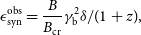 \begin{align} \epsilon^{\mathrm{obs}}_{\mathrm{syn}} = \frac{B}{B_{\mathrm{cr}}}\gamma^2_{\mathrm{b}}\delta/(1+z), \end{align}
 \begin{align} \epsilon^{\mathrm{obs}}_{\mathrm{EC}} = \frac{4}{3}\epsilon_{\mathrm{0,ext}}\gamma^2_{\mathrm{b}}\delta^2/(1+z), \end{align}
respectively (Coppi & Blandford Reference Coppi and Blandford1990; Tavecchio et al. Reference Tavecchio, Maraschi and Ghisellini1998; Ghisellini & Tavecchio Reference Ghisellini and Tavecchio2008a), where B is the magnetic field strength in units of Gauss; $\gamma_{\mathrm{b}}$
is the break Lorentz factor of relativistic electrons responsible for the SED peaks;
$\gamma_{\mathrm{b}}$
is the break Lorentz factor of relativistic electrons responsible for the SED peaks; $\epsilon_{\mathrm{0,ext}}$
is the dimensionless energy of ambient soft photons in the AGN frame;
$\epsilon_{\mathrm{0,ext}}$
is the dimensionless energy of ambient soft photons in the AGN frame; $B_{\mathrm{cr}} = m_e^2c^3/e\hbar$
is the critical magnetic field strength;
$B_{\mathrm{cr}} = m_e^2c^3/e\hbar$
is the critical magnetic field strength; $\delta = [\Gamma(1-\beta \cos \theta_{\mathrm{obs}})]^{-1}$
is the Doppler factor, where
$\delta = [\Gamma(1-\beta \cos \theta_{\mathrm{obs}})]^{-1}$
is the Doppler factor, where $\Gamma$
is the bulk Lorentz factor,
$\Gamma$
is the bulk Lorentz factor, $\beta c$
is the jet speed, and
$\beta c$
is the jet speed, and $\theta_{\mathrm{obs}}$
is the viewing angle. In this paper, by assuming
$\theta_{\mathrm{obs}}$
is the viewing angle. In this paper, by assuming $\theta_{\mathrm{obs}} \lesssim 1 / \Gamma$
, we have
$\theta_{\mathrm{obs}} \lesssim 1 / \Gamma$
, we have $\delta \approx \Gamma$
. It is worth noting that equation (2) is only applicable within the Thomson regime.
$\delta \approx \Gamma$
. It is worth noting that equation (2) is only applicable within the Thomson regime.
Dividing equation (1) by equation (2), we obtain
 \begin{align} \frac{B}{\delta} = \frac{4B_{\mathrm{cr}} \epsilon_{\mathrm{0,ext}} \epsilon^{\mathrm{obs}}_{\mathrm{syn}}}{3\epsilon^{\mathrm{obs}}_{\mathrm{EC}}}. \end{align}
And the peak luminosities of synchrotron radiation and EC scattering in the observer’s frame can be written as
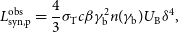 \begin{align} L^{\mathrm{obs}}_{\mathrm{syn,p}} = \frac{4}{3}\sigma_{\mathrm{T}}c\beta \gamma_{\mathrm{b}}^2n(\gamma_{\mathrm{b}})U_{\mathrm{B}}\delta^4, \end{align}
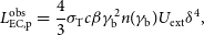 \begin{align} L^{\mathrm{obs}}_{\mathrm{EC,p}} = \frac{4}{3}\sigma_{\mathrm{T}}c\beta \gamma_{\mathrm{b}}^2n(\gamma_{\mathrm{b}})U_{\mathrm{ext}}\delta^4, \end{align}
respectively (Blumenthal & Gould Reference Blumenthal and Gould1970; Rybicki, Lightman, & Tayler Reference Rybicki, Lightman and Tayler1981), where $\sigma_{\mathrm{T}}$
is the Thomson cross section;
$\sigma_{\mathrm{T}}$
is the Thomson cross section; $n(\gamma_{\mathrm{b}})$
is the electron density distribution at
$n(\gamma_{\mathrm{b}})$
is the electron density distribution at $\gamma_{\mathrm{b}}$
;
$\gamma_{\mathrm{b}}$
; $U_{\mathrm{B}} = B^2/8\pi$
is the energy density of the magnetic field. Here, the energy density of the ambient photon fields in the comoving frame can be calculated as
$U_{\mathrm{B}} = B^2/8\pi$
is the energy density of the magnetic field. Here, the energy density of the ambient photon fields in the comoving frame can be calculated as
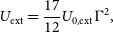 \begin{align} U_{\mathrm{ext}} = \frac{17}{12}U_{\mathrm{0,ext}}\Gamma^2, \end{align}
where $U_{\mathrm{0,ext}}$
is the energy density in the AGN frame (Ghisellini & Tavecchio Reference Ghisellini and Tavecchio2008c; Ghisellini & Tavecchio Reference Ghisellini and Tavecchio2008b).
$U_{\mathrm{0,ext}}$
is the energy density in the AGN frame (Ghisellini & Tavecchio Reference Ghisellini and Tavecchio2008c; Ghisellini & Tavecchio Reference Ghisellini and Tavecchio2008b).
Take the ratio of equations (4) and (5), we then get
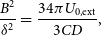 \begin{align} \frac{B^2}{\delta^2} = \frac{34 \pi U_{\mathrm{0,ext}}}{3\textit{CD}}, \end{align}
where $\textit{CD} = \textit{L}^{\mathrm{obs}}_{\mathrm{EC,p}}/\textit{L}^{\mathrm{obs}}_{\mathrm{syn,p}}$
is the Compton dominance.
$\textit{CD} = \textit{L}^{\mathrm{obs}}_{\mathrm{EC,p}}/\textit{L}^{\mathrm{obs}}_{\mathrm{syn,p}}$
is the Compton dominance.
Combining equations (3) and (7), we ultimately derive the seed factor as
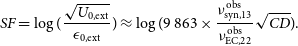 \begin{align} {\textit{SF}} = \log(\frac{\sqrt{\textit{U}_{\mathrm{0,ext}}}}{\epsilon _{\mathrm{0,ext}}}) \approx \log(9\,863 \times \frac{\nu ^{\mathrm{obs}}_{\mathrm{syn,13}}}{\nu ^{\mathrm{obs}}_{\mathrm{EC,22}}}\sqrt{\textit{CD}}). \end{align}
Here, $\nu^{\mathrm{obs}}_{\mathrm{syn,13}}$
is the peak frequency of synchrotron radiation in units of 1013 Hz and
$\nu^{\mathrm{obs}}_{\mathrm{syn,13}}$
is the peak frequency of synchrotron radiation in units of 1013 Hz and $\nu^{\mathrm{obs}}_{\mathrm{EC,22}}$
is the peak frequency of EC scattering in units of 1022 Hz.
$\nu^{\mathrm{obs}}_{\mathrm{EC,22}}$
is the peak frequency of EC scattering in units of 1022 Hz.
2.2 Characteristic values of the seed factor
As the ambient photon fields, the BLR and DT were discussed in the former seed factor approach (Georganopoulos et al. Reference Georganopoulos, Meyer and Fossati2012; Harvey et al. Reference Harvey, Georganopoulos and Meyer2020; Huang et al. Reference Huang, Li, Liao, Huang, Li, Qian, Pei and Fan2022). In addition, some studies revealed the significance of CMB and starlight (Böttcher et al. Reference Böttcher, Dermer and Finke2008; Potter & Cotter, Reference Potter and Cotter2013a,b,c). In this work, we comprehensively consider the seed factors of BLR, DT, CMB, and starlight. The accretion disc is out of consideration, because it is not suitable to this method.
To calculate the characteristic seed factor of BLR, the energy density $U_{\mathrm{0,ext}}$
and the dimensionless energy
$U_{\mathrm{0,ext}}$
and the dimensionless energy $\epsilon_{\mathrm{0,ext}}$
of the soft photons need to be determined. The typical size of BLR is
$\epsilon_{\mathrm{0,ext}}$
of the soft photons need to be determined. The typical size of BLR is $R_{\mathrm{BLR}} \approx 1 \times 10^{17} L_{\mathrm{d,45}}^{1/2} \ \mathrm{cm}$
, where
$R_{\mathrm{BLR}} \approx 1 \times 10^{17} L_{\mathrm{d,45}}^{1/2} \ \mathrm{cm}$
, where $L_{\mathrm{d, 45}}$
is the luminosity of the accretion disc in units of
$L_{\mathrm{d, 45}}$
is the luminosity of the accretion disc in units of $10^{45} \mathrm{erg \ s^{-1}}$
(Kaspi et al. Reference Kaspi, Brandt, Maoz, Netzer, Schneider and Shemmer2007; Bentz et al. Reference Bentz, Peterson, Netzer, Pogge and Vestergaard2009). The covering factor of BLR (the fractions of the disc luminosity
$10^{45} \mathrm{erg \ s^{-1}}$
(Kaspi et al. Reference Kaspi, Brandt, Maoz, Netzer, Schneider and Shemmer2007; Bentz et al. Reference Bentz, Peterson, Netzer, Pogge and Vestergaard2009). The covering factor of BLR (the fractions of the disc luminosity $L_{\mathrm{d}}$
reprocessed into the BLR radiation) is
$L_{\mathrm{d}}$
reprocessed into the BLR radiation) is $\xi_{\mathrm{BLR}} = 0.1$
(Ghisellini & Tavecchio Reference Ghisellini and Tavecchio2009). We then obtain the energy density
$\xi_{\mathrm{BLR}} = 0.1$
(Ghisellini & Tavecchio Reference Ghisellini and Tavecchio2009). We then obtain the energy density $U_{\mathrm{0, BLR}} = \xi_{\mathrm{BLR}}L_{\mathrm{d}}/4\pi R_{\mathrm{BLR}}^2c = 2.65\times10^{-2}\mathrm{erg \ cm^{-3}}$
within the characteristic distance. The BLR can be regarded as a grey body with peak frequency of
$U_{\mathrm{0, BLR}} = \xi_{\mathrm{BLR}}L_{\mathrm{d}}/4\pi R_{\mathrm{BLR}}^2c = 2.65\times10^{-2}\mathrm{erg \ cm^{-3}}$
within the characteristic distance. The BLR can be regarded as a grey body with peak frequency of $1.5 {\nu}_{{\mathrm{Ly}}_{\alpha} }$
, then the dimensionless photon energy is
$1.5 {\nu}_{{\mathrm{Ly}}_{\alpha} }$
, then the dimensionless photon energy is $\epsilon_{\mathrm{0,BLR}} = 3\times10^{-5}$
(Tavecchio & Ghisellini Reference Tavecchio and Ghisellini2008). Finally, with a 5% uncertainty, we derive the characteristic seed factor of BLR as
$\epsilon_{\mathrm{0,BLR}} = 3\times10^{-5}$
(Tavecchio & Ghisellini Reference Tavecchio and Ghisellini2008). Finally, with a 5% uncertainty, we derive the characteristic seed factor of BLR as ${\textit{SF}}_{\mathrm{BLR}} = 3.74 \pm 0.19$
.
${\textit{SF}}_{\mathrm{BLR}} = 3.74 \pm 0.19$
.
The typical size of DT is found to be $R_{\mathrm{DT}} \approx 2.5\times10^{18} L_{\mathrm{d,45}}^{1/2} \ \mathrm{cm}$
(Ghisellini & Tavecchio Reference Ghisellini and Tavecchio2009; Pei et al. Reference Pei, Fan, Yang, Huang and Li2022). In this work, we set the covering factor of DT as
$R_{\mathrm{DT}} \approx 2.5\times10^{18} L_{\mathrm{d,45}}^{1/2} \ \mathrm{cm}$
(Ghisellini & Tavecchio Reference Ghisellini and Tavecchio2009; Pei et al. Reference Pei, Fan, Yang, Huang and Li2022). In this work, we set the covering factor of DT as $\xi_{\mathrm{DT}} = 0.5$
(Ghisellini & Tavecchio Reference Ghisellini and Tavecchio2009). Then the energy density of DT within the characteristic distance is
$\xi_{\mathrm{DT}} = 0.5$
(Ghisellini & Tavecchio Reference Ghisellini and Tavecchio2009). Then the energy density of DT within the characteristic distance is $U_{\mathrm{0, DT}} = \xi_{\mathrm{DT}} L_{\mathrm{d}}/4\pi R_{\mathrm{DT}}^2 c = 2.12 \times 10^{-4} \mathrm{erg\ cm^{-3}}$
. In the studies, the DT, which can also be approximated by a grey body, is endowed with three different temperatures, for example, 80K (Lopez-Rodriguez et al. Reference Lopez-Rodriguez2018), 370K (Ghisellini & Tavecchio Reference Ghisellini and Tavecchio2009), 1 500K (Almeyda et al. Reference Almeyda, Robinson, Richmond, Vazquez and Nikutta2017; Lyu & Rieke Reference Lyu and Rieke2018). Then we obtain three dimensionless photon energies for the DT, which are
$U_{\mathrm{0, DT}} = \xi_{\mathrm{DT}} L_{\mathrm{d}}/4\pi R_{\mathrm{DT}}^2 c = 2.12 \times 10^{-4} \mathrm{erg\ cm^{-3}}$
. In the studies, the DT, which can also be approximated by a grey body, is endowed with three different temperatures, for example, 80K (Lopez-Rodriguez et al. Reference Lopez-Rodriguez2018), 370K (Ghisellini & Tavecchio Reference Ghisellini and Tavecchio2009), 1 500K (Almeyda et al. Reference Almeyda, Robinson, Richmond, Vazquez and Nikutta2017; Lyu & Rieke Reference Lyu and Rieke2018). Then we obtain three dimensionless photon energies for the DT, which are $\epsilon_{\mathrm{0,DT}}^{\mathrm{80\,K}} = 5.30 \times 10^{-8},\ \epsilon_{\mathrm{0,DT}}^{\mathrm{370K}} = 2.45\times 10^{-7}, \ \epsilon_{\mathrm{0,DT}}^{\mathrm{1\,500\,K}} = 9.94\times 10^{-7}$
. Considering the 5% uncertainty, three distinct characteristic seed factors of DT can be described as follows:
$\epsilon_{\mathrm{0,DT}}^{\mathrm{80\,K}} = 5.30 \times 10^{-8},\ \epsilon_{\mathrm{0,DT}}^{\mathrm{370K}} = 2.45\times 10^{-7}, \ \epsilon_{\mathrm{0,DT}}^{\mathrm{1\,500\,K}} = 9.94\times 10^{-7}$
. Considering the 5% uncertainty, three distinct characteristic seed factors of DT can be described as follows: ${\textit{SF}}_{\mathrm{DT}}^{\mathrm{80\,K}} = 5.44 \pm 0.27, \ {\textit{SF}}_{\mathrm{DT}}^{\mathrm{370\,K}} = 4.77\pm 0.24,\ {\textit{SF}}_{\mathrm{DT}}^{\mathrm{1\,500\,K}} = 4.17 \pm 0.21$
.
${\textit{SF}}_{\mathrm{DT}}^{\mathrm{80\,K}} = 5.44 \pm 0.27, \ {\textit{SF}}_{\mathrm{DT}}^{\mathrm{370\,K}} = 4.77\pm 0.24,\ {\textit{SF}}_{\mathrm{DT}}^{\mathrm{1\,500\,K}} = 4.17 \pm 0.21$
.
For CMB, the energy density is $U_{\mathrm{CMB}} = 4.02\times10^{-13}\mathrm{erg\ cm^{-3}}$
and the typical temperature is
$U_{\mathrm{CMB}} = 4.02\times10^{-13}\mathrm{erg\ cm^{-3}}$
and the typical temperature is $T_{\mathrm{CMB}} = 2.72\,{\mathrm{K}}$
in the observer’s frame, respectively (Böttcher et al. Reference Böttcher, Dermer and Finke2008). In this case, the characteristic seed factor of CMB with 5% uncertainty is
$T_{\mathrm{CMB}} = 2.72\,{\mathrm{K}}$
in the observer’s frame, respectively (Böttcher et al. Reference Böttcher, Dermer and Finke2008). In this case, the characteristic seed factor of CMB with 5% uncertainty is ${\textit{SF}}_{\mathrm{CMB}} = 2.55\pm0.13$
. The energy density for starlight is
${\textit{SF}}_{\mathrm{CMB}} = 2.55\pm0.13$
. The energy density for starlight is $U_{\mathrm{0,SL}} = 8.01 \times 10^{-13} \mathrm{erg\ cm^{-3}}$
and the typical temperature is
$U_{\mathrm{0,SL}} = 8.01 \times 10^{-13} \mathrm{erg\ cm^{-3}}$
and the typical temperature is $T_{\mathrm{SL}} = 30\,{\mathrm{K}}$
. Then we get the characteristic seed factor of starlight with 5% uncertainty
$T_{\mathrm{SL}} = 30\,{\mathrm{K}}$
. Then we get the characteristic seed factor of starlight with 5% uncertainty ${\textit{SF}}_{\mathrm{SL}} = 1.65\pm0.08$
(H. E. S. S. Collaboration et al. 2017).
${\textit{SF}}_{\mathrm{SL}} = 1.65\pm0.08$
(H. E. S. S. Collaboration et al. 2017).
When applying the seed factor approach, there are several caveats that should be kept in mind. Firstly, the preceding derivation of the seed factor is within the Thomson regime. As a result of $\gamma \epsilon \lt 1/4$
(Moderski et al. Reference Moderski, Sikora, Coppi and Aharonian2005), the corresponding peak frequency of the EC radiation belonging to BLR, DT, CMB and starlight must be less than
$\gamma \epsilon \lt 1/4$
(Moderski et al. Reference Moderski, Sikora, Coppi and Aharonian2005), the corresponding peak frequency of the EC radiation belonging to BLR, DT, CMB and starlight must be less than $1.03\times 10^{25}[\epsilon_0(1+z)/10^{-6}]^{-1}\,\mathrm{Hz}$
. Since high-energy component of LSP usually peaks around 1 GeV, the EC process associated to BLR occurs in the Klein-Nishina regime, while others are cooling in the Thomson regime. Then the available energy density of BLR could reduce and the actual characteristic seed factor of BLR would be smaller than the above derived one. Secondly, the energy density of the BLR and DT could be smaller at farther site as proposed by Hayashida et al. (Reference Hayashida2012), that is,
$1.03\times 10^{25}[\epsilon_0(1+z)/10^{-6}]^{-1}\,\mathrm{Hz}$
. Since high-energy component of LSP usually peaks around 1 GeV, the EC process associated to BLR occurs in the Klein-Nishina regime, while others are cooling in the Thomson regime. Then the available energy density of BLR could reduce and the actual characteristic seed factor of BLR would be smaller than the above derived one. Secondly, the energy density of the BLR and DT could be smaller at farther site as proposed by Hayashida et al. (Reference Hayashida2012), that is,
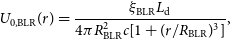 \begin{align} U_{\mathrm{0,BLR}}(r) = \frac{\xi_{\mathrm{BLR}} L_{\mathrm{d}}}{4\pi R^2_{\mathrm{BLR}}c[1+(r/R_{\mathrm{BLR}})^3]}, \end{align}
and
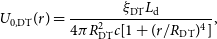 \begin{align} U_{\mathrm{0,DT}}(r) = \frac{\xi_{\mathrm{DT}} L_{\mathrm{d}}}{4\pi R^2_{\mathrm{DT}}c[1+(r/R_{\mathrm{DT}})^4]},\end{align}
where r is the distance between the dissipation region and the central black hole, both energy densities of the BLR and DT have been transformed into the AGN frame (see also Fig. 1). Then the actual characteristic seed factor could also be smaller if the emission region is beyond the typical distance. Since the above derived characteristic seed factor of DT is the largest one among these four photon fields, the actual seed factor of DT covers that of the others. For example, the actual seed factor of DT could decrease to about 3.5 and equal to the actual seed factor of BLR. Therefore, the above derived seed factor of DT but not of BLR, CMB, or starlight is effective. If the observed seed factor is approximated to the derived $\textit{SF}_{\mathrm{DT}}$
, it can be ascertained that the DT dominates the soft photon fields.
$\textit{SF}_{\mathrm{DT}}$
, it can be ascertained that the DT dominates the soft photon fields.
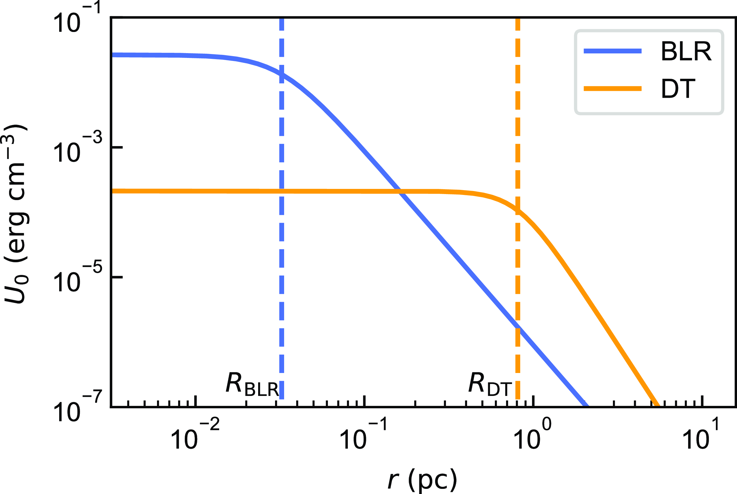
Figure 1. Energy density distribution of the broad line region (BLR) and the dusty torus (DT). $L_{\mathrm{d}} = 1\times 10^{45} {\mathrm{erg\ s^{-1}}}$
is adopted.
$L_{\mathrm{d}} = 1\times 10^{45} {\mathrm{erg\ s^{-1}}}$
is adopted.
2.3 The fitting of spectral energy distribution
As shown in equation (8), the observed seed factor can be determined by extracting the peak frequencies and luminosities associated with the two humps. Then we fit each SED by the quadratic and cubic functions, respectively. Namely,
 \begin{align} \left\{ \begin{aligned} &\log(\nu F _{\nu}) = a_2(\log \nu)^2 + b_2\log \nu + c_2,\\ &\log(\nu F _{\nu}) = a_3(\log \nu)^3 + b_3(\log \nu)^2 + c_3\log \nu + d_3. \end{aligned}\right.\end{align}
We use two kinds of functions because some SEDs possess high symmetry but others do not, which causes difference on the parameters (Xue et al. Reference Xue2016). Markov-chain Monte Carlo (MCMC) analysis is employed since it returns robust uncertainties on the parameters (Speagle Reference Speagle2019). It works by randomly sampling from the posterior distribution, which are derived from the product of prior distribution and likelihood function. We use an uninformative uniform prior distribution because we have little knowledge about the parameters of quadratic and cubic functions in advance. Conservatively, it is expressed by
 \begin{align}p(m) = \left\{ \begin{aligned} &\frac{1}{1\,000}, &{\mathrm{if}}\ m_0-500 \lt m \lt m_0+500\\ &0, &\mathrm{otherwise} \end{aligned}\right.\end{align}
where m denotes the paremeters in both quadratic and cubic functions, such as $a_2, b_2 ...$
And
$a_2, b_2 ...$
And $m_0$
is the preprocessed m derived by numpy.polyfit.Footnote
a
The likelihood function is written as (Yamada et al. Reference Yamada, Uemura, Itoh, Fukazawa, Ohno and Imazato2020)
$m_0$
is the preprocessed m derived by numpy.polyfit.Footnote
a
The likelihood function is written as (Yamada et al. Reference Yamada, Uemura, Itoh, Fukazawa, Ohno and Imazato2020)
 \begin{align} {\textit{L}} = \prod_{i=1}^n \frac{1}{\sqrt{2 \pi {\sigma_i}^2}} \exp{\left(-\frac{ ({\nu} F _{\nu,i} - \nu F _{\nu}(\nu_i))^2}{2\sigma^2_i} \right)}.\end{align}
Here, $\sigma_i$
is the Gaussian error of data point i and n is the number of data points in each energy hump. The emcee Python packageFootnote
b
(version 3.1.2, Foreman-Mackey et al. Reference Foreman-Mackey, Hogg, Lang and Goodman2013) is utilised to perform the MCMC algorithm. This package employs an affine invariant MCMC ensemble sampler with interdependent chains (Goodman & Weare Reference Goodman and Weare2010). While there is no fixed number of samples needed to make the convergence, we evaluate the convergence by inspecting the corner plot of parameters. The autocorrelation time, also the time that the chain ‘forgets’ where it started, range from 35 to 250 in our Python program. Conservatively, we adopt 32 walkers (chains) initialised by the above preprocessed values with a
$\sigma_i$
is the Gaussian error of data point i and n is the number of data points in each energy hump. The emcee Python packageFootnote
b
(version 3.1.2, Foreman-Mackey et al. Reference Foreman-Mackey, Hogg, Lang and Goodman2013) is utilised to perform the MCMC algorithm. This package employs an affine invariant MCMC ensemble sampler with interdependent chains (Goodman & Weare Reference Goodman and Weare2010). While there is no fixed number of samples needed to make the convergence, we evaluate the convergence by inspecting the corner plot of parameters. The autocorrelation time, also the time that the chain ‘forgets’ where it started, range from 35 to 250 in our Python program. Conservatively, we adopt 32 walkers (chains) initialised by the above preprocessed values with a $10^{-10}$
Gaussian error, run 17 000 steps, burn 2 000 steps, and thin by 25. The results of posterior distribution are presented in Fig. 2.
$10^{-10}$
Gaussian error, run 17 000 steps, burn 2 000 steps, and thin by 25. The results of posterior distribution are presented in Fig. 2.
While fitting the SEDs, we also compare the goodness of the two different function models with modified Akaike Information Criterion (AICc; Akaike Reference Akaike1974; Burnham & Anderson Reference Burnham and Anderson2002), written as
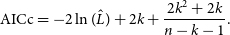 \begin{align} {\mathrm{AICc}} = -2\ln(\hat{L}) + 2k + \frac{2k^2+2k} {n-k-1}.\end{align}
In this formula, $\hat{L}$
is the maximum likelihood, which corresponds to the maximum posterior since we used an uniform prior, and k is the number of free parameters. This criterion is chosen because the sample size of data points is small. AICc evaluates the loss of information during the fitting. The smaller AICc means the better model. Actually, the additional parameters in a model should improve the fitting to the data points, but we should also consider the increase in model complexity which causes overfitting. In this case, the AICc includes a penalty.
$\hat{L}$
is the maximum likelihood, which corresponds to the maximum posterior since we used an uniform prior, and k is the number of free parameters. This criterion is chosen because the sample size of data points is small. AICc evaluates the loss of information during the fitting. The smaller AICc means the better model. Actually, the additional parameters in a model should improve the fitting to the data points, but we should also consider the increase in model complexity which causes overfitting. In this case, the AICc includes a penalty.

Figure 2. Posterior distribution from the Markov-chain Monte Carlo analysis of OD 166’s low-energy (synchrotron) hump with quadratic function. We present only one corner plot here, those of other SEDs are available in machine-readable form.
2.4 Parameters of the emission region
By fitting the SEDs of blazars, the observed peak frequencies and peak luminosities are determined. Then we select the blazars whose seed factors fall within the $\textit{SF}_{\mathrm{DT}}$
. With the gathered information on variability timescales and Doppler factors, we can deduce the other physical parameters of the
$\textit{SF}_{\mathrm{DT}}$
. With the gathered information on variability timescales and Doppler factors, we can deduce the other physical parameters of the $\gamma$
-ray emission region. For blazars, we have such a formula (Tavecchio et al. Reference Tavecchio, Maraschi and Ghisellini1998; Nalewajko, Begelman, & Sikora Reference Nalewajko, Begelman and Sikora2014):
$\gamma$
-ray emission region. For blazars, we have such a formula (Tavecchio et al. Reference Tavecchio, Maraschi and Ghisellini1998; Nalewajko, Begelman, & Sikora Reference Nalewajko, Begelman and Sikora2014):
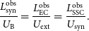 \begin{align} \frac{L^{\mathrm{obs}}_{\mathrm{syn}}}{U_{\mathrm{B}}} = \frac{L^{\mathrm{obs}}_{\mathrm{EC}}}{U_{\mathrm{ext}}} = \frac{L^{\mathrm{obs}}_{\mathrm{SSC}}}{U_{\mathrm{syn}}}.\end{align}
Here, $L^{\mathrm{obs}}_{\mathrm{syn}}$
,
$L^{\mathrm{obs}}_{\mathrm{syn}}$
, $L^{\mathrm{obs}}_{\mathrm{EC}}$
,
$L^{\mathrm{obs}}_{\mathrm{EC}}$
, $L^{\mathrm{obs}}_{\mathrm{SSC}}$
are the luminosities of the synchrotron, EC, and SSC radiations, respectively.
$L^{\mathrm{obs}}_{\mathrm{SSC}}$
are the luminosities of the synchrotron, EC, and SSC radiations, respectively. $L^{\mathrm{obs}}_{\mathrm{syn}}$
and
$L^{\mathrm{obs}}_{\mathrm{syn}}$
and $L^{\mathrm{obs}}_{\mathrm{EC}}$
are determined by the integral of the low-energy and high-energy humps, respectively. For simplicity, we boldly assume that
$L^{\mathrm{obs}}_{\mathrm{EC}}$
are determined by the integral of the low-energy and high-energy humps, respectively. For simplicity, we boldly assume that $L^{\mathrm{obs}}_{\mathrm{SSC}} = 10 \times L^{\mathrm{obs}}_{\mathrm{X}}$
, where
$L^{\mathrm{obs}}_{\mathrm{SSC}} = 10 \times L^{\mathrm{obs}}_{\mathrm{X}}$
, where $L^{\mathrm{obs}}_{\mathrm{X}}$
is the maximum luminosity in X-ray band.
$L^{\mathrm{obs}}_{\mathrm{X}}$
is the maximum luminosity in X-ray band. $U_{\mathrm{syn}} = L^{\mathrm{obs}}_{\mathrm{syn}}/( 4\pi R^2c\delta^4 )$
is the energy density of the synchrotron radiation. The radius of the
$U_{\mathrm{syn}} = L^{\mathrm{obs}}_{\mathrm{syn}}/( 4\pi R^2c\delta^4 )$
is the energy density of the synchrotron radiation. The radius of the $\gamma$
-ray emission region in the comoving frame can be estimated as
$\gamma$
-ray emission region in the comoving frame can be estimated as
 \begin{align} R \approx ct_{\mathrm{var}}\frac{\delta}{1+z},\end{align}
where $t_{\mathrm{var}}$
is the variablility timescale.
$t_{\mathrm{var}}$
is the variablility timescale.
If we have measured the variability timescale, we can derive the following parameters by combining the above formulas:
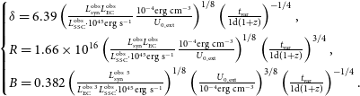 \begin{align} \begin{cases} \delta = 6.39 \left( \frac{L^{\mathrm{obs}}_{\mathrm{syn}} L^{\mathrm{obs}}_{\mathrm{EC}}}{L^{\mathrm{obs}}_{\mathrm{SSC}} \cdot 10^{45} \mathrm{erg \ s^{-1}}} \frac{\mathrm{10^{-4}erg\ cm^{-3}}}{U_{\mathrm{0,ext}}}\right)^{1/8} \left(\frac{t_{\mathrm{var}}}{1\mathrm{d}(1+z)} \right)^{-1/4},\\[5pt] R = 1.66\times 10^{16} \left( \frac{L^{\mathrm{obs}}_{\mathrm{syn}} L^{\mathrm{obs}}_{\mathrm{EC}}}{L^{\mathrm{obs}}_{\mathrm{SSC}} \cdot 10^{45} \mathrm{erg \ s^{-1}} } \frac{\mathrm{10^{-4}erg\ cm^{-3}}}{U_{\mathrm{0,ext}}} \right)^{1/8} \left( \frac{t_{\mathrm{var}}}{1 \mathrm{d}(1+z)} \right)^{3/4},\\[5pt] B = 0.382 \left( \frac{L^{\mathrm{obs} \ 5}_{\mathrm{syn}}}{L^{\mathrm{obs} \ 3}_{\mathrm{EC}} L^{\mathrm{obs}}_{\mathrm{SSC}} \cdot 10^{45}\mathrm{erg\ s^{-1}}} \right)^{1/8} \left( \frac{U_{\mathrm{0,ext}}}{\mathrm{10^{-4}erg\ cm^{-3}}}\right) ^{3/8} \left( \frac{t_{\mathrm{var}}}{\mathrm{1d}(1+z)} \right)^{-1/4}.\end{cases}\end{align}
When the Doppler factor is measured, we obtain:
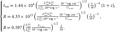 \begin{align}\begin{cases} t_{\mathrm{var}} = 1.44\times10^{4} \left( \frac{L^{\mathrm{obs}}_{\mathrm{syn}} L^{\mathrm{obs}}_{\mathrm{EC}}}{L^{\mathrm{obs}}_{\mathrm{SSC}} \cdot 10^{45} \mathrm{erg\ s^{-s}}} \frac{\mathrm{10^{-4}erg\ cm^{-3}}}{U_{\mathrm{0,ext}}} \right)^{1/2} \left( \frac{\delta}{10} \right)^{-4} (1+z),\\[5pt] R = 4.33 \times 10^{15} \left( \frac{L^{\mathrm{obs}}_{\mathrm{syn}} L^{\mathrm{obs}}_{\mathrm{EC}}}{L^{\mathrm{obs}}_{\mathrm{SSC}} \cdot \mathrm{10^{45}erg\ s^{-1}}} \frac{\mathrm{10^{-4}erg\ cm^{-3}}}{U_{\mathrm{{0,ext}}}}\right) ^{1/2} \left( \frac{\delta}{10} \right) ^{-3},\\[5pt] B = 0.597 \left( \frac{L^{\mathrm{obs}}_{\mathrm{syn}}}{L^{\mathrm{obs}}_{\mathrm{EC}}} \frac{U_{\mathrm{0,ext}}}{\mathrm{10^{-4}erg\ cm^{-3}}}\right)^{1/2} \frac{\delta}{10}.\end{cases}\end{align}
Besides, $\gamma_{\mathrm{b}}$
can be calculated by Tavecchio et al. (Reference Tavecchio, Maraschi and Ghisellini1998)
$\gamma_{\mathrm{b}}$
can be calculated by Tavecchio et al. (Reference Tavecchio, Maraschi and Ghisellini1998)
 \begin{align}\gamma_{\mathrm{b}} = 5.2\times10^{-4} \left( \frac{\nu^{\mathrm{obs}}_{\mathrm{syn}}(1+z)}{B\delta} \right)^{1/2}.\end{align}
2.5 Constraint of the internal $\gamma \gamma$
-absorption
$\gamma \gamma$
-absorption

To make a comprison with the above derivation of physical parameters, we further make a constraint on $\delta$
through
$\delta$
through $\gamma\gamma$
-absorption (see also Dondi & Ghisellini Reference Dondi and Ghisellini1995). Due to the
$\gamma\gamma$
-absorption (see also Dondi & Ghisellini Reference Dondi and Ghisellini1995). Due to the $\gamma\gamma$
annihilation, electron-positron pairs are generated. Applying Delta-approximation, the corresponding optical depth can be calculated as (Foffano et al. Reference Foffano, Vittorini, Tavani and Menegoni2022):
$\gamma\gamma$
annihilation, electron-positron pairs are generated. Applying Delta-approximation, the corresponding optical depth can be calculated as (Foffano et al. Reference Foffano, Vittorini, Tavani and Menegoni2022):
 \begin{align} \tau_{\gamma\gamma} = \sigma_{\gamma\gamma}n_{\mathrm{soft}}R,\end{align}
where $n_{\mathrm{soft}} = U_{\mathrm{soft}}/h\nu_{\mathrm{soft}}$
is the number density of the soft photons and
$n_{\mathrm{soft}} = U_{\mathrm{soft}}/h\nu_{\mathrm{soft}}$
is the number density of the soft photons and $\sigma_{\gamma\gamma} = 1.68 \times 10^{-25} \mathrm{cm ^2}$
is the
$\sigma_{\gamma\gamma} = 1.68 \times 10^{-25} \mathrm{cm ^2}$
is the $\gamma \gamma$
-absorption cross section, which is assumed to be a constant when such a condition is fulfilled:
$\gamma \gamma$
-absorption cross section, which is assumed to be a constant when such a condition is fulfilled:
 \begin{align}\epsilon_{\mathrm{soft}}\epsilon_{\gamma} =2,\end{align}
where $\epsilon_{\mathrm{soft}}$
and
$\epsilon_{\mathrm{soft}}$
and $\epsilon_{\gamma}$
are the dimensionless energies of the soft photons and
$\epsilon_{\gamma}$
are the dimensionless energies of the soft photons and $\gamma$
-ray photons (comoving frame), respectively (Dermer & Menon Reference Dermer and Menon2009).
$\gamma$
-ray photons (comoving frame), respectively (Dermer & Menon Reference Dermer and Menon2009).
Since the $\gamma$
-ray is detected, optical depth must be less than 1. In order to solve the optical depth, energy density need to be determined. For internal soft photon fields such as synchrotron and IC radiation, we employ
$\gamma$
-ray is detected, optical depth must be less than 1. In order to solve the optical depth, energy density need to be determined. For internal soft photon fields such as synchrotron and IC radiation, we employ
 \begin{align} U_{\mathrm{soft}} = \frac{\nu L^{\mathrm{obs}}_{\nu, {\mathrm{soft}}}}{4\pi R^2c\delta^4}, \end{align}
where $\nu L^{\mathrm{obs}} _{\nu, {\mathrm{soft}}} = 4\pi d_{\mathrm{L}}^2 \nu F^{\mathrm{obs}}_{\nu,{\mathrm{soft}}}$
is the observed luminosity of the soft photons,
$\nu L^{\mathrm{obs}} _{\nu, {\mathrm{soft}}} = 4\pi d_{\mathrm{L}}^2 \nu F^{\mathrm{obs}}_{\nu,{\mathrm{soft}}}$
is the observed luminosity of the soft photons, $d_{\mathrm{L}}$
is the luminosity distance, and
$d_{\mathrm{L}}$
is the luminosity distance, and $\nu F^{\mathrm{obs}}_{\nu,{\mathrm{soft}}}$
is the observed flux. Then we derive
$\nu F^{\mathrm{obs}}_{\nu,{\mathrm{soft}}}$
is the observed flux. Then we derive
 \begin{align} \tau_{\gamma\gamma} = \frac{\sigma_{\gamma\gamma}d^2_{\mathrm{L}}\nu F^{\mathrm{obs}}_{\nu,{\mathrm{soft}}(1+z)}}{hc^2t_{\mathrm{var}}\delta^5\nu_{\mathrm{soft}}} \lt 1.\end{align}
Here, $\nu_{\mathrm{soft}}$
could be derived from equation (21) and expressed by
$\nu_{\mathrm{soft}}$
could be derived from equation (21) and expressed by
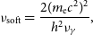 \begin{align} \nu_{\mathrm{soft}} = \frac{2(m_{\mathrm{e}}c^2)^2}{h^2\nu_{\gamma}},\end{align}
where $\nu_{\gamma} = \nu_{\gamma}^{\mathrm{obs}}(1+z)/\delta$
is the frequency of
$\nu_{\gamma} = \nu_{\gamma}^{\mathrm{obs}}(1+z)/\delta$
is the frequency of $\gamma$
-ray in the comoving frame. Then we obtain the lower limit of
$\gamma$
-ray in the comoving frame. Then we obtain the lower limit of $\delta$
:
$\delta$
:
 \begin{align} \delta \gt \left( \frac{h\sigma_{\gamma\gamma}d_{\mathrm{L}}^2\nu F_{\nu,{\mathrm{soft}}}^{\mathrm{obs}}\nu_{\gamma}^{\mathrm{obs}}(1+z)^2}{2m_{\mathrm{e}}^2c^6t_{\mathrm{var}}} \right)^{1/6}. \end{align}
Not only do internal photon fields constrain the physical parameter, but external photon fields also give an additional constraint on r. The absorption of DT could be omitted according to equation (21), since the corresponding $\gamma$
-ray (
$\gamma$
-ray ( $\nu_{\gamma}^{\mathrm{obs}} = 10^{27}(\nu_{\mathrm{DT}}/10^{13} \mathrm{Hz})^{-1}\mathrm{Hz}$
) is beyond detection in our collected SEDs. However, the
$\nu_{\gamma}^{\mathrm{obs}} = 10^{27}(\nu_{\mathrm{DT}}/10^{13} \mathrm{Hz})^{-1}\mathrm{Hz}$
) is beyond detection in our collected SEDs. However, the $\gamma$
-ray up to
$\gamma$
-ray up to $10^{25}(\nu_{\mathrm{BLR}}/10^{15} \mathrm{Hz})^{-1}\mathrm{Hz}$
that is detectable could be absorbed by BLR. Therefore, we inspect the
$10^{25}(\nu_{\mathrm{BLR}}/10^{15} \mathrm{Hz})^{-1}\mathrm{Hz}$
that is detectable could be absorbed by BLR. Therefore, we inspect the $\gamma\gamma$
-absorption of BLR by unfolding its frequency spectrum. Given that the BLR is a grey body, we have
$\gamma\gamma$
-absorption of BLR by unfolding its frequency spectrum. Given that the BLR is a grey body, we have
 \begin{align} \frac{\mathrm{d}\textit{U}}{{\mathrm{d}} \nu} = \frac{8\pi h \nu^3}{c^3}(e^{h\nu / k_{\mathrm{B}}T}-1)^{-1}, \end{align}
where $T = h\nu_{\mathrm{BLR}}/3.93k_{\mathrm{B}}$
is the characteristic temperature of BLR and
$T = h\nu_{\mathrm{BLR}}/3.93k_{\mathrm{B}}$
is the characteristic temperature of BLR and $k_{\mathrm{B}}$
is the Boltzmann constant (Ghisellini & Tavecchio Reference Ghisellini and Tavecchio2009). From the combination of equations (9) and (26), we derive the energy density of BLR as a function of both r and
$k_{\mathrm{B}}$
is the Boltzmann constant (Ghisellini & Tavecchio Reference Ghisellini and Tavecchio2009). From the combination of equations (9) and (26), we derive the energy density of BLR as a function of both r and $\nu$
:
$\nu$
:
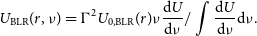 \begin{align} U_{\mathrm{BLR}}(r,\nu) = \Gamma^2 U_{\mathrm{0,BLR}}(r)\nu \frac{\mathrm{d} \textit{U}}{{\mathrm{d}} \nu} / \int \frac{\mathrm{d} \textit{U}}{{\mathrm{d}} \nu}{\mathrm{d}}\nu.\end{align}
With the same condition about $\tau \lt 1$
and lower limit of
$\tau \lt 1$
and lower limit of $\delta$
derived from equation (25), we could get the lower limit of r:
$\delta$
derived from equation (25), we could get the lower limit of r:
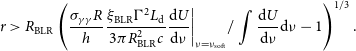 \begin{align} r \gt R_{\mathrm{BLR}} \left( \frac{\sigma_{\gamma\gamma}R}{h} \frac{\xi_{\mathrm{BLR}} \Gamma^2L_{\mathrm{d}}}{3\pi R^2_{\mathrm{BLR}}c} \frac{\mathrm{d} \textit{U}}{{\mathrm{d}} \nu} \bigg|_{\nu = \nu_{\mathrm{soft}}}/ \int\frac{\mathrm{d} \textit{U}}{{\mathrm{d}} \nu}\mathrm{d}\nu -1 \right)^{1/3}.\end{align}
3. Application
3.1 Low-synchrotron-peaked blazars
Locating the $\gamma$
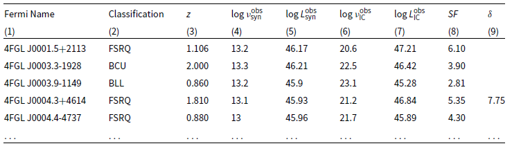
-ray emission region of blazars has been a significant issue in the Fermi era. Debates continuously happen because of the limited accuracy of instruments and complicated radiation mechanism of blazars. In this work, we adopted the seed factor approach proposed by Georganopoulos et al. (Reference Georganopoulos, Meyer and Fossati2012). Based on the derivation in Section 2.1, some observed quantities need to be determined. We collected a sample of 1 138 LSPs with synchrotron peak frequencies and luminosities from Yang et al. (Reference Yang2022), and with IC peak frequencies and luminosities from Yang et al. (Reference Yang2023). There are 630 FSRQs, 132 BL Lacs and 376 blazar candidates of uncertain type (BCUs) in this sample (see also Table 1). The Doppler factors of 383 blazars are also recorded from Liodakis et al. (Reference Liodakis, Hovatta, Huppenkothen, Kiehlmann, Max-Moerbeck and Readhead2018) for further calculation. Fig. 3 displays the histogram of observed seed factors belonging to the LSPs, which is obtained using equation (8). The observed seed factors of FSRQs and BCUs converge around the areas of DT, which demonstrates that DT dominates the soft photon fields of FSRQs and BCUs. This can be attributed to the strong radiation from DT, which is reproduced by the strong radiation from accretion disc of FSRQs and BCUs (Madejski & Sikora Reference Madejski2016; Huang et al. Reference Huang, Li, Liao, Huang, Li, Qian, Pei and Fan2022). The observed seed factors of BL Lacs converge around the area of BLR. This suggests that the soft photons either originate from BLR or from DT, as the actual seed factor of DT could be smaller than the one depicted in Fig. 3. The areas of CMB and starlight appear on the left edge of the histogram, indicating that their contributions to the soft photons in the EC process are relatively small. In general, observed seed factors of 552 in 1 138 LSPs directly fall into the areas of DT, which locates the
$\gamma$
-ray emission region of blazars has been a significant issue in the Fermi era. Debates continuously happen because of the limited accuracy of instruments and complicated radiation mechanism of blazars. In this work, we adopted the seed factor approach proposed by Georganopoulos et al. (Reference Georganopoulos, Meyer and Fossati2012). Based on the derivation in Section 2.1, some observed quantities need to be determined. We collected a sample of 1 138 LSPs with synchrotron peak frequencies and luminosities from Yang et al. (Reference Yang2022), and with IC peak frequencies and luminosities from Yang et al. (Reference Yang2023). There are 630 FSRQs, 132 BL Lacs and 376 blazar candidates of uncertain type (BCUs) in this sample (see also Table 1). The Doppler factors of 383 blazars are also recorded from Liodakis et al. (Reference Liodakis, Hovatta, Huppenkothen, Kiehlmann, Max-Moerbeck and Readhead2018) for further calculation. Fig. 3 displays the histogram of observed seed factors belonging to the LSPs, which is obtained using equation (8). The observed seed factors of FSRQs and BCUs converge around the areas of DT, which demonstrates that DT dominates the soft photon fields of FSRQs and BCUs. This can be attributed to the strong radiation from DT, which is reproduced by the strong radiation from accretion disc of FSRQs and BCUs (Madejski & Sikora Reference Madejski2016; Huang et al. Reference Huang, Li, Liao, Huang, Li, Qian, Pei and Fan2022). The observed seed factors of BL Lacs converge around the area of BLR. This suggests that the soft photons either originate from BLR or from DT, as the actual seed factor of DT could be smaller than the one depicted in Fig. 3. The areas of CMB and starlight appear on the left edge of the histogram, indicating that their contributions to the soft photons in the EC process are relatively small. In general, observed seed factors of 552 in 1 138 LSPs directly fall into the areas of DT, which locates the $\gamma$
-ray emission region at 1–10 pc.
$\gamma$
-ray emission region at 1–10 pc.
Table 1. Observed quantities and seed factors of 1138 low-synchrotron-peaked blazars.
Note: Column (1) gives the Fermi name. Column (2) represents the spectral classification. Column (3) gives the redshift. Column (4) and (5) are the synchrotron peak frequencies and luminosities from Yang et al. (Reference Yang2022), respectively. Column (6) and (7) are the IC peak frequencies and luminosities from Yang et al. (Reference Yang2023), respectively. Column (8) gives the observed seed factors. Column (9) gives the Doppler factors of 383 blazars from Liodakis et al. (Reference Liodakis, Hovatta, Huppenkothen, Kiehlmann, Max-Moerbeck and Readhead2018). We present only 5 items here, full table is available in machine-readable form.
Figure 3. Histogram of observed seed factors. FSRQs, BL Lacs, and blazar candidates of uncertain type (BCU) in our sample are distinguished by three kinds of grids. Three red areas represent the scales of characteristic seed factors belonging to the dusty torus (DT) in three different temperatures. Blue, green, and yellow areas represent the scales of characteristic seed factors belonging to the broad line region (BLR), cosmic microwave background (CMB) and starlight (SL).
This result is consistent with the former analysis using the seed factor approach. Harvey et al. (Reference Harvey, Georganopoulos and Meyer2020) calculated the seed factors of 62 FSRQs and found the distribution peaking at a value corresponding to DT. Huang et al. (Reference Huang, Li, Liao, Huang, Li, Qian, Pei and Fan2022) used a sample of 619 sources and also found the distribution is located at DT. In our work, rather than setting the temperature of DT to 1 200 K, we considered three different temperatures of DT because it is a relatively thick gas cloud with its inner temperature varying from the outer one (Lyu & Rieke Reference Lyu and Rieke2018). Fig. 3 shows 370 K dominates the distribution of observed seed factors, indicating most $\gamma$
-ray emission regions are located inside the DT.
$\gamma$
-ray emission regions are located inside the DT.
3.2 LSPs dominated by the dusty torus
Although our result suggests that DT dominates the soft photon fields of LSPs, previous study demonstrated that blazars might have various $\gamma$
-ray emission regions in different flare epochs (Dotson et al. Reference Dotson, Georganopoulos, Meyer and McCann2015). We investigated this property by collecting some historical flare states. LSPs whose observed seed factors directly fall into the red areas in Fig. 3 (i.e. LSPs dominated by the DT) were selected, since only their soft photon fields had been determined effectively. The SEDs that we collected fulfilled these conditions: Possessing multi-wavelength quasi-simultaneous data except for the radio band. The observation times of each band intersect within two months. In total, we collected 23 SEDs. The related references are given in Table 2. These SEDs were fitted by both quadratic and cubic functions using the MCMC method (see also Figs. A1 & A2). Then we extracted the peak frequencies and luminosities of two humps and calculated the observed seed factors. The results are displayed as scatterplots in Fig. 4. The distributions of data scatters vary under two different function fits. This demonstrates that the values of seed factors are significantly influenced by the choice of the function. On the other hand, both fitting results of two different functions show that some scatters, that is, 7 scatters of quadratic function and 9 scatters of cubic function, move outside DT areas. Although the actual seed factor of DT could be smaller and cover them, they have already moved to the areas of BLR or CMB. This indicates that the location of
$\gamma$
-ray emission regions in different flare epochs (Dotson et al. Reference Dotson, Georganopoulos, Meyer and McCann2015). We investigated this property by collecting some historical flare states. LSPs whose observed seed factors directly fall into the red areas in Fig. 3 (i.e. LSPs dominated by the DT) were selected, since only their soft photon fields had been determined effectively. The SEDs that we collected fulfilled these conditions: Possessing multi-wavelength quasi-simultaneous data except for the radio band. The observation times of each band intersect within two months. In total, we collected 23 SEDs. The related references are given in Table 2. These SEDs were fitted by both quadratic and cubic functions using the MCMC method (see also Figs. A1 & A2). Then we extracted the peak frequencies and luminosities of two humps and calculated the observed seed factors. The results are displayed as scatterplots in Fig. 4. The distributions of data scatters vary under two different function fits. This demonstrates that the values of seed factors are significantly influenced by the choice of the function. On the other hand, both fitting results of two different functions show that some scatters, that is, 7 scatters of quadratic function and 9 scatters of cubic function, move outside DT areas. Although the actual seed factor of DT could be smaller and cover them, they have already moved to the areas of BLR or CMB. This indicates that the location of $\gamma$
-ray emission region changed in historical flare states, and the soft photon fields could transition from DT to BLR and CMB.
$\gamma$
-ray emission region changed in historical flare states, and the soft photon fields could transition from DT to BLR and CMB.
Table 2. Results of parameter analysis.
Note: Column (1) and (2) give the Fermi name and source name, respectively. The sources marked with $^{*}$
are the DT dominated LSPs with observed Doppler factors, and the others possess observed variability timescales. Column (3) gives the observed time period. Column (4) gives the observed or derived variability timescales. Column (5) gives the observed or derived Doppler factors. Column (6), (7), and (8) are the derived magnetic field strength, the derived radius of emission region and the derived break Lorentz factor of relativistic electrons, respectively. Column (9) and (10) give the lower limits of Doppler factors and distance between the black hole and emission region, which are derived from internal
$^{*}$
are the DT dominated LSPs with observed Doppler factors, and the others possess observed variability timescales. Column (3) gives the observed time period. Column (4) gives the observed or derived variability timescales. Column (5) gives the observed or derived Doppler factors. Column (6), (7), and (8) are the derived magnetic field strength, the derived radius of emission region and the derived break Lorentz factor of relativistic electrons, respectively. Column (9) and (10) give the lower limits of Doppler factors and distance between the black hole and emission region, which are derived from internal $\gamma\gamma$
absorption. Column (11) is the related reference. The table contains some rows with double sub-rows. The upper one is the parameter obtained by fitting SEDs with quadratic function, and the lower one is the parameter obtained by fitting SEDs with cubic function. References: (1) Sahakyan et al. (Reference Sahakyan, Israyelyan, Harutyunyan, Khachatryan and Gas-paryan2020); (2) Ghisellini et al. (Reference Ghisellini, Tavecchio, Foschini, Ghirlanda, Maraschi and Celotti2010); (3) Tan et al. (Reference Tan, Xue, Du, Xi, Wang and Xie2020); (4) Sahakyan et al. (Reference Sahakyan, Israyelyan, Harutyunyan, Khachatryan and Gas-paryan2020); (5) Ammenadka et al. (Reference Ammenadka, Bhattacharya, Bhattacharyya, Bhatt and Stalin2022); (6) Das, Mondal, & Prince (Reference Das, Mondal and Prince2023); (7) Palma et al. (Reference Palma2011); (8) Orienti et al. (Reference Orienti, D’Ammando, Giroletti, Finke, Ajello, Dallacasa and Venturi2014); (9) Das, Prince, & Gupta (Reference Das, Prince and Gupta2020); (10) Roy et al. (Reference Roy, Patel, Sarkar, Chatterjee and Chitnis2021); (11) Dutka et al. (Reference Dutka2017); (12) D’Ammando et al. (Reference D’Ammando2012); (13) Malik et al. (Reference Malik, Shah, Sahayanathan, Iqbal and Manzoor2022); (14) Patel et al. (Reference Patel, Bose, Gupta and Zuberi2021); (15) Hayashida et al. (Reference Hayashida2015); (16) Fraija et al. (Reference Fraija, Bentez, Hiriart, Sorcia, López, Mújica, Cabr-era and Galván-Gámez2019); (17) Zacharias et al. (Reference Zacharias, Böttcher, Jankowsky, Lenain, Wagner and Wierzcholska2017); (18) Pacciani et al. (Reference Pacciani, Tavecchio, Donnarumma, Stamerra, Carrasco, Recillas, Porras and Uemura2014); (19) Gasparyan et al. (Reference Gasparyan, Sahakyan, Baghmanyan and Zargaryan2018); (20) Prince et al. (Reference Prince, Raman, Hahn, Gupta and Majumdar2018); (21) Zacharias et al. (Reference Zacharias, Böttcher, Jankowsky, Lenain, Wagner and Wierzcholska2019); (22) Sahakyan (Reference Sahakyan2020); (23) Acciari et al. (Reference Acciari2022); (24) Sahakyan (Reference Sahakyan2018); (25) Oikonomou et al. (Reference Oikonomou, Murase, Padovani, Resconi and Mészáros2019); (26) Chen & Bai (Reference Chen and Bai2010); (27) Kushwaha, Sahayanathan, & Singh (Reference Kushwaha, Sahayanathan and Singh2013).
$\gamma\gamma$
absorption. Column (11) is the related reference. The table contains some rows with double sub-rows. The upper one is the parameter obtained by fitting SEDs with quadratic function, and the lower one is the parameter obtained by fitting SEDs with cubic function. References: (1) Sahakyan et al. (Reference Sahakyan, Israyelyan, Harutyunyan, Khachatryan and Gas-paryan2020); (2) Ghisellini et al. (Reference Ghisellini, Tavecchio, Foschini, Ghirlanda, Maraschi and Celotti2010); (3) Tan et al. (Reference Tan, Xue, Du, Xi, Wang and Xie2020); (4) Sahakyan et al. (Reference Sahakyan, Israyelyan, Harutyunyan, Khachatryan and Gas-paryan2020); (5) Ammenadka et al. (Reference Ammenadka, Bhattacharya, Bhattacharyya, Bhatt and Stalin2022); (6) Das, Mondal, & Prince (Reference Das, Mondal and Prince2023); (7) Palma et al. (Reference Palma2011); (8) Orienti et al. (Reference Orienti, D’Ammando, Giroletti, Finke, Ajello, Dallacasa and Venturi2014); (9) Das, Prince, & Gupta (Reference Das, Prince and Gupta2020); (10) Roy et al. (Reference Roy, Patel, Sarkar, Chatterjee and Chitnis2021); (11) Dutka et al. (Reference Dutka2017); (12) D’Ammando et al. (Reference D’Ammando2012); (13) Malik et al. (Reference Malik, Shah, Sahayanathan, Iqbal and Manzoor2022); (14) Patel et al. (Reference Patel, Bose, Gupta and Zuberi2021); (15) Hayashida et al. (Reference Hayashida2015); (16) Fraija et al. (Reference Fraija, Bentez, Hiriart, Sorcia, López, Mújica, Cabr-era and Galván-Gámez2019); (17) Zacharias et al. (Reference Zacharias, Böttcher, Jankowsky, Lenain, Wagner and Wierzcholska2017); (18) Pacciani et al. (Reference Pacciani, Tavecchio, Donnarumma, Stamerra, Carrasco, Recillas, Porras and Uemura2014); (19) Gasparyan et al. (Reference Gasparyan, Sahakyan, Baghmanyan and Zargaryan2018); (20) Prince et al. (Reference Prince, Raman, Hahn, Gupta and Majumdar2018); (21) Zacharias et al. (Reference Zacharias, Böttcher, Jankowsky, Lenain, Wagner and Wierzcholska2019); (22) Sahakyan (Reference Sahakyan2020); (23) Acciari et al. (Reference Acciari2022); (24) Sahakyan (Reference Sahakyan2018); (25) Oikonomou et al. (Reference Oikonomou, Murase, Padovani, Resconi and Mészáros2019); (26) Chen & Bai (Reference Chen and Bai2010); (27) Kushwaha, Sahayanathan, & Singh (Reference Kushwaha, Sahayanathan and Singh2013).
3.3 Four typical low-synchrotron-peaked blazars
In order to further verify the alteration of $\gamma$
-ray emission region in different flare epochs, we collected SEDs of four typical LSPs, including 7 SEDs of CTA 102, 7 SEDs of 3C 279, 3 SEDs of TXS 0506+056, and 5 SEDs of OJ 287. The references of these SEDs are presented in Table 2. These SEDs fulfilled the same conditions as above. Similarly, we fitted these SEDs with both quadratic and cubic functions (see also Figs. A3–A6), extracted the peak frequencies and luminosities, and created the scatterplots of observed seed factors (see also Fig. 5). The scatter distributions still vary significantly under two different function fits. Fig. 5 also shows that the observed seed factors of the same LSPs are variable in different flare states. Some scatters are positioned in red areas, while others are not, indicating multiple locations of
$\gamma$
-ray emission region in different flare epochs, we collected SEDs of four typical LSPs, including 7 SEDs of CTA 102, 7 SEDs of 3C 279, 3 SEDs of TXS 0506+056, and 5 SEDs of OJ 287. The references of these SEDs are presented in Table 2. These SEDs fulfilled the same conditions as above. Similarly, we fitted these SEDs with both quadratic and cubic functions (see also Figs. A3–A6), extracted the peak frequencies and luminosities, and created the scatterplots of observed seed factors (see also Fig. 5). The scatter distributions still vary significantly under two different function fits. Fig. 5 also shows that the observed seed factors of the same LSPs are variable in different flare states. Some scatters are positioned in red areas, while others are not, indicating multiple locations of $\gamma$
-ray emission regions in the same blazar. Some previous studies also support our results. Patiño-Álvarez et al. (Reference Patiño-Álvarez2018) collected multi-wavelength light curves for 3C 279 over 6 yr and divided them into three flaring periods. They analysed the time delays and
$\gamma$
-ray emission regions in the same blazar. Some previous studies also support our results. Patiño-Álvarez et al. (Reference Patiño-Álvarez2018) collected multi-wavelength light curves for 3C 279 over 6 yr and divided them into three flaring periods. They analysed the time delays and $\gamma$
-ray spectral index, then found that the dominant radiation mechanism and
$\gamma$
-ray spectral index, then found that the dominant radiation mechanism and $\gamma$
-ray emission regions varied in different periods. Similar to the above LSPs, Deng & Jiang (Reference Deng and Jiang2023) located the
$\gamma$
-ray emission regions varied in different periods. Similar to the above LSPs, Deng & Jiang (Reference Deng and Jiang2023) located the $\gamma$
-ray emission region of OT 081 at the edge of BLR during the 2016 multiwavelength flare and at about 1–10 pc away from the black hole during the 2009–2012 orphan X-ray flare. Given to the variability of blazars, broadtime analysis has become a typical approach of Fermi-LAT to reduce the impact of some short-lived flares (Arsioli & Polenta Reference Arsioli and Polenta2018).
$\gamma$
-ray emission region of OT 081 at the edge of BLR during the 2016 multiwavelength flare and at about 1–10 pc away from the black hole during the 2009–2012 orphan X-ray flare. Given to the variability of blazars, broadtime analysis has become a typical approach of Fermi-LAT to reduce the impact of some short-lived flares (Arsioli & Polenta Reference Arsioli and Polenta2018).
On September 22 2017, the IceCube Observatory detected a $\sim$
290 TeV neutrino from the direction of TXS 0506+056 (IceCube Collaboration et al. 2018; Padovani et al. Reference Padovani, Giommi, Resconi, Glauch, Arsioli, Sahakyan and Huber2018). The neutrino was produced in the photopion process, in which the
$\sim$
290 TeV neutrino from the direction of TXS 0506+056 (IceCube Collaboration et al. 2018; Padovani et al. Reference Padovani, Giommi, Resconi, Glauch, Arsioli, Sahakyan and Huber2018). The neutrino was produced in the photopion process, in which the $\triangle^{+}(1232)$
resonance contributes the main cross section. Using Delta-approximation, we could derive the external soft photon energy in the AGN frame,
$\triangle^{+}(1232)$
resonance contributes the main cross section. Using Delta-approximation, we could derive the external soft photon energy in the AGN frame,
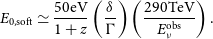 \begin{align} E_{\mathrm{0, soft}} \simeq \frac{50 {\mathrm{eV}}}{1+z} \left(\frac{\delta}{\Gamma}\right) \left( \frac{290{\mathrm{TeV}}}{E^{\mathrm{obs}}_{\nu}}\right).\end{align}
It shows that the dissipation region was in the BLR. This neutrino event was closely followed by two very high energy $\gamma$
-ray flares of TXS 0506+056 (Ansoldi et al. Reference Ansoldi2018; Sahakyan Reference Sahakyan2018). These flares were denoted as Flare 2 and Flare 3 in Fig. 5. The seed factors are presented in Fig. A5, corresponding to serial number 2 and 3. Result of quadratic function depects that the dissipation region was in the DT, contradicting the above calculation. But that of cubic function approximately supports the BLR. This manifests the difference between two functions and possible superiority of cubic function.
$\gamma$
-ray flares of TXS 0506+056 (Ansoldi et al. Reference Ansoldi2018; Sahakyan Reference Sahakyan2018). These flares were denoted as Flare 2 and Flare 3 in Fig. 5. The seed factors are presented in Fig. A5, corresponding to serial number 2 and 3. Result of quadratic function depects that the dissipation region was in the DT, contradicting the above calculation. But that of cubic function approximately supports the BLR. This manifests the difference between two functions and possible superiority of cubic function.
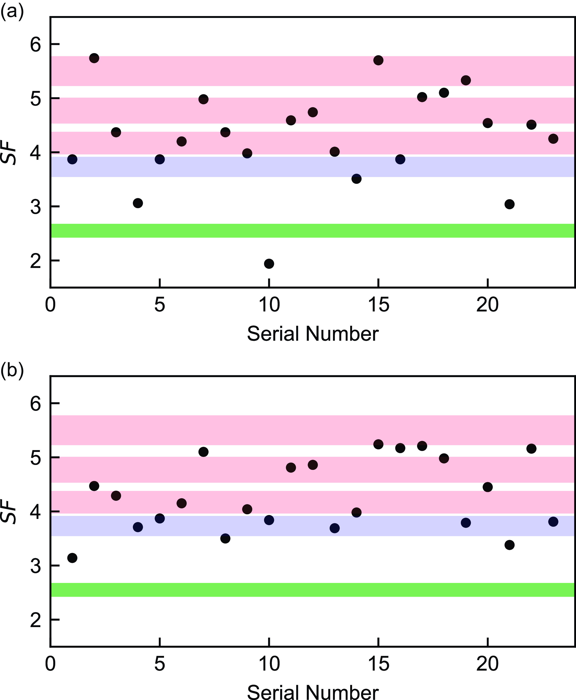
Figure 4. Scatterplots of observed seed factors belonging to low-synchrotron-peaked blazars dominated by the dusty torus. These data correspond to the first 23 flare states in Table 0, ordered from top to bottom. The upper and lower panels are derived from SEDs fitted by quadratic and cubic functions, respectively. Red, blue, and green areas depict the characteristic seed factors of dusty torus, broad line region, and cosmic microwave background, respectively.
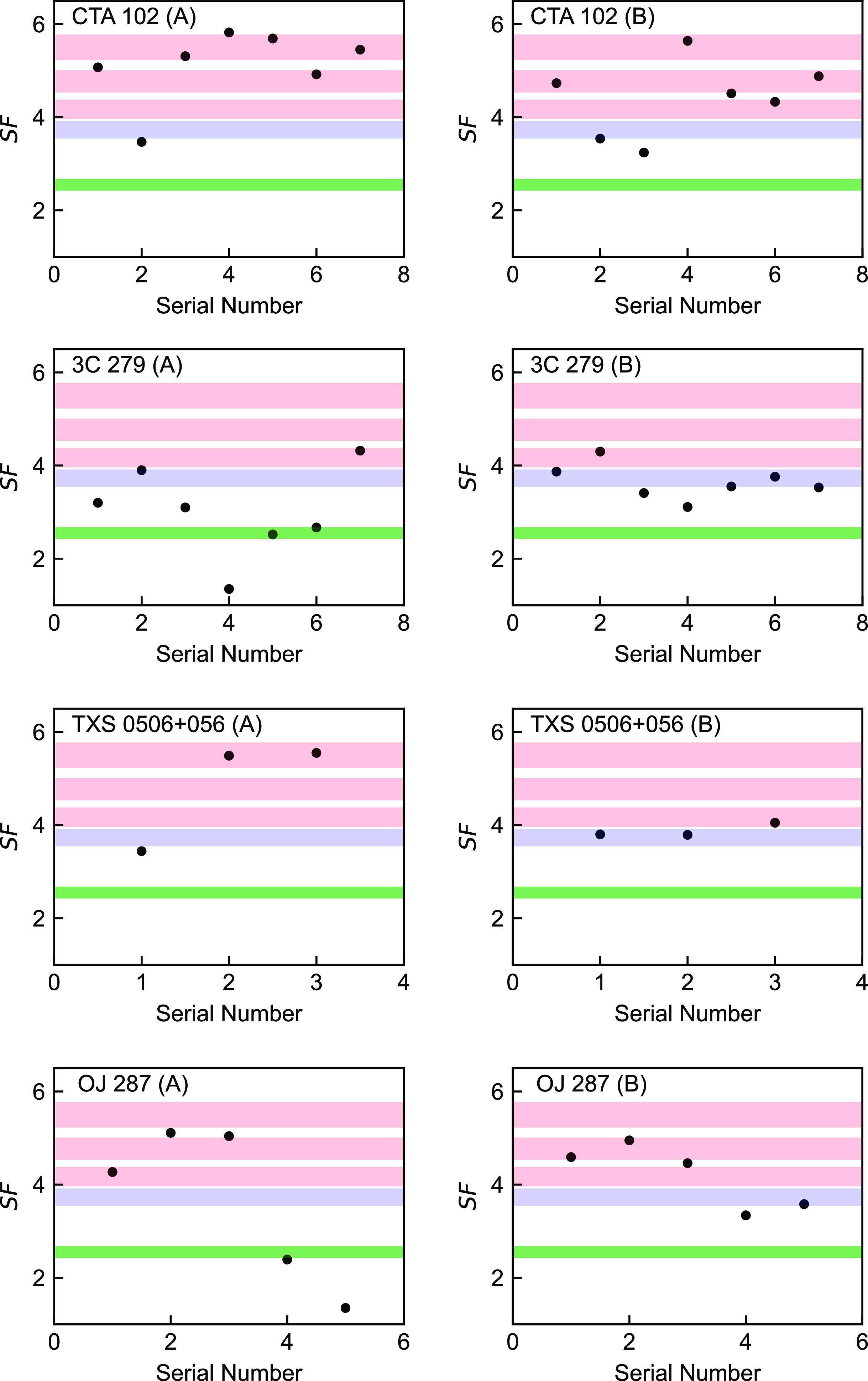
Figure 5. From top to bottom, the scatterplots represent the observed seed factor distributions of historical states for CTA 102, 3C 279, TXS 0506+056, and OJ 287, respectively. The left and right panels are derived from SEDs fitted by quadratic and cubic functions, respectively. Red, blue, and green areas depict the characteristic seed factors of dusty torus, broad line region and cosmic microwave background, respectively.
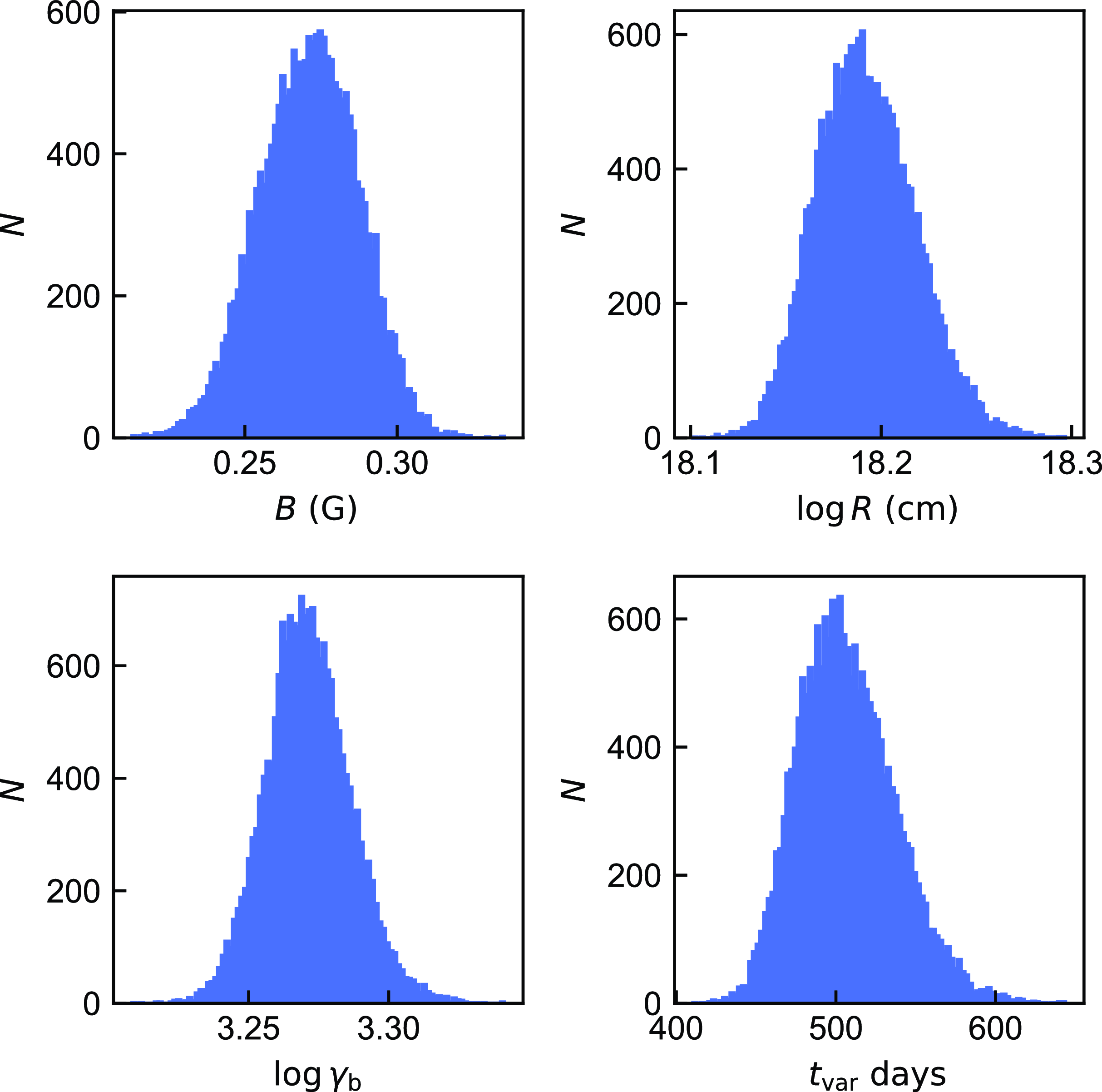
Figure 6. Parameter distribution of OD 166 when Doppler factor is known. Possible value counts of each parameter is 19 200 (=32 $\times$
(17 000-2 000)/25) in total. The number of bins is 100. We present only one sample here, others are available in machine-readable form.
$\times$
(17 000-2 000)/25) in total. The number of bins is 100. We present only one sample here, others are available in machine-readable form.
3.4 Model comparison and parameter analysis
We found that different authors adopted various functions to fit the SEDs. Abdo et al. (Reference Abdo2010c) employed the cubic function, while Chen (Reference Chen2014), Yang et al. (Reference Yang2022, Reference Yang2023) used a simpler quadratic function. Xue et al. (Reference Xue2016) fitted the Synchrotron hump with both functions and found the derived Synchrotron luminosity with cubic function is lower. In this work, we tried both of the two to further illuminate the difference. The AICc of each hump derived from two functions are presented on the figures in Appendix. For the low-energy humps, 33 (45 in total, one is null because $n=k+1$
) AICc of cubic function are smaller. As for high-energy humps, 35 (45 in total) AICc of cubic function are smaller. This demonstrates a dominance of cubic function over quadratic function both in two kinds of humps. We found that the humps with perfect symmetry could be fitted well (i.e. smaller AICc) with quadratic function, such as low-energy humps in PKS 2123-463, OJ 287 Flare 3, OJ 287 Flare 4, etc., and high-energy humps in PKS 0208-512 Flare 1, PKS 0402-362 Flare 2, PKS 0420+022, etc. The asymmetrical SEDs, which take the most part of our samples, could be explained well with cubic function. On the other hand, we found some quadratic function curves deviate badly from the GeV data points, such as PKS 0208-512 Flare 2, TXS 0506+056 Flare 1, and NARO 512. It is worth noting that GeV data is rarer than other wavebands’ in practical, given that the
$n=k+1$
) AICc of cubic function are smaller. As for high-energy humps, 35 (45 in total) AICc of cubic function are smaller. This demonstrates a dominance of cubic function over quadratic function both in two kinds of humps. We found that the humps with perfect symmetry could be fitted well (i.e. smaller AICc) with quadratic function, such as low-energy humps in PKS 2123-463, OJ 287 Flare 3, OJ 287 Flare 4, etc., and high-energy humps in PKS 0208-512 Flare 1, PKS 0402-362 Flare 2, PKS 0420+022, etc. The asymmetrical SEDs, which take the most part of our samples, could be explained well with cubic function. On the other hand, we found some quadratic function curves deviate badly from the GeV data points, such as PKS 0208-512 Flare 2, TXS 0506+056 Flare 1, and NARO 512. It is worth noting that GeV data is rarer than other wavebands’ in practical, given that the $\gamma$
-ray telescopes are relatively scarce. Thus the goodness of fit of data points in GeV band has superiority. For 3C 279 Flare 4 and CTA 102 Flare 3, the quadratic function curves in high-energy hump even continuedly increase, which breaks the physical reality. Therefore, we recommend the cubic function to fit the SEDs.
$\gamma$
-ray telescopes are relatively scarce. Thus the goodness of fit of data points in GeV band has superiority. For 3C 279 Flare 4 and CTA 102 Flare 3, the quadratic function curves in high-energy hump even continuedly increase, which breaks the physical reality. Therefore, we recommend the cubic function to fit the SEDs.
However, cubic function is not suitable to all the SEDs, such as high-energy humps in TXS 0536+145 and CTA 102 Flare 3 (see Appendix). The hard $\gamma$
-ray spectra and lack of higher-energy data make it difficult to form a full peak. We also noticed that the conventional one-zone leptonic or hadronic model could hardly explain the SEDs of bright TeV blazars, which results in extreme values (Abdo et al. Reference Abdo2011;Cerruti et al. Reference Cerruti, Zech, Boisson and Inoue2015; Li et al. Reference Li, Xue, Long, Wang, Nagataki, Yan and Wang2022). In this case, some models of inhomogeneous jet were constructed, such as spine-layer model (Ghisellini, Tavecchio, & Chiaberge Reference Ghisellini, Tavecchio and Chiaberge2005; Tavecchio & Ghisellini Reference Tavecchio and Ghisellini2014), two-zone leptonic model (Shukla et al. Reference Shukla2015) and twozone leptohadronic model (Aguilar-Ruiz et al. Reference Aguilar-Ruiz, Fraija, Galván-Gámez and Bentez2022).
$\gamma$
-ray spectra and lack of higher-energy data make it difficult to form a full peak. We also noticed that the conventional one-zone leptonic or hadronic model could hardly explain the SEDs of bright TeV blazars, which results in extreme values (Abdo et al. Reference Abdo2011;Cerruti et al. Reference Cerruti, Zech, Boisson and Inoue2015; Li et al. Reference Li, Xue, Long, Wang, Nagataki, Yan and Wang2022). In this case, some models of inhomogeneous jet were constructed, such as spine-layer model (Ghisellini, Tavecchio, & Chiaberge Reference Ghisellini, Tavecchio and Chiaberge2005; Tavecchio & Ghisellini Reference Tavecchio and Ghisellini2014), two-zone leptonic model (Shukla et al. Reference Shukla2015) and twozone leptohadronic model (Aguilar-Ruiz et al. Reference Aguilar-Ruiz, Fraija, Galván-Gámez and Bentez2022).
Besides collecting the quasi-simultaneous data and fitting the SEDs, we collected the corresponding Doppler factor from Liodakis et al. (Reference Liodakis, Hovatta, Huppenkothen, Kiehlmann, Max-Moerbeck and Readhead2018) or observed variability timescales from the original work and obtained the distribution of some related parameters using formulas in Section 2.4. For example, Fig. 6 presents the derived parameter distribution of OD 166 when the corresponding Doppler factor from Liodakis et al. (Reference Liodakis, Hovatta, Huppenkothen, Kiehlmann, Max-Moerbeck and Readhead2018) is known. There are 19 200 possible values for each parameter from the MCMC fitting. The 16-50-84 percentile rule is employed to characterise parameter uncertainty. The detailed results of parameter analysis are listed in Table 2. The average value for variability timescale, Doppler factor, magnetic field strength, radius of emission region, and break Lorentz factor of electrons are 36.58 days, 23.40, 0.674 G, $3.540\times10^{16}$
cm, and 845.28, respectively. Table 2 shows that the physical parameters of a specific blazar changed in different flaring epochs. Feng et al. (Reference Feng, Hu, Zhou and Gao2022) reproduced the SEDs of various flares belonging to 3C 454.3 under a one-zone leptonic scenario and found similar variations in physical parameters. Interestingly, Table 2 demonstrates that parameters under two different function fits are analogous, which is unlike the scatterplots. This could be attributed to the effect of symmetry in two humps. It causes more influences in peak frequencies which are mainly used to calculate the observed seed factors, but less in the integral of two humps which are used to calculate the other parameters. We also constrained the Doppler factors and r for the collected LSPs whose observed timescales are known. Table 2 depicts that all the former derived Doppler factors are consistent with their corresponding lower limit. We noticed that some lower limits of r equal to 0. Because the results of derivation in Section 2.5 are negative numbers, but r must be non-negative numbers in real world. This indicates that the constraint of internal
$3.540\times10^{16}$
cm, and 845.28, respectively. Table 2 shows that the physical parameters of a specific blazar changed in different flaring epochs. Feng et al. (Reference Feng, Hu, Zhou and Gao2022) reproduced the SEDs of various flares belonging to 3C 454.3 under a one-zone leptonic scenario and found similar variations in physical parameters. Interestingly, Table 2 demonstrates that parameters under two different function fits are analogous, which is unlike the scatterplots. This could be attributed to the effect of symmetry in two humps. It causes more influences in peak frequencies which are mainly used to calculate the observed seed factors, but less in the integral of two humps which are used to calculate the other parameters. We also constrained the Doppler factors and r for the collected LSPs whose observed timescales are known. Table 2 depicts that all the former derived Doppler factors are consistent with their corresponding lower limit. We noticed that some lower limits of r equal to 0. Because the results of derivation in Section 2.5 are negative numbers, but r must be non-negative numbers in real world. This indicates that the constraint of internal $\gamma\gamma$
-absorption on r is relatively weak.
$\gamma\gamma$
-absorption on r is relatively weak.
4. Conclusions
In this work, we calculated the observed seed factors of 1138 LSPs and the characteristic seed factors of four external photon fields, then plotted the histogram distribution to locate the $\gamma$
-ray emission region. SEDs related to historical flare states were collected to investigate the variable locations. These SEDs were fitted by both quadratic and cubic functions using the MCMC method. Furthermore, we derived some parameters of emission region and employed a constraint of internal
$\gamma$
-ray emission region. SEDs related to historical flare states were collected to investigate the variable locations. These SEDs were fitted by both quadratic and cubic functions using the MCMC method. Furthermore, we derived some parameters of emission region and employed a constraint of internal $\gamma \gamma$
-absorption to verify the derivation. Our main results are as follows:
$\gamma \gamma$
-absorption to verify the derivation. Our main results are as follows:
-
1. We find that DT dominates the soft photon fields of LSPs and
$\gamma$
-ray emission regions of LSPs are mainly located at 1–10 pc. Histogram shows that the corresponding distribution of BL Lacs peaks at the area of BLR, but this area could also be covered by the actual value of DT. CMB and starlight make little contribution to the
$\gamma$
-ray emission of LSPs. -
2. The locations of
$\gamma$
-ray emission region of LSPs are variable in different flare epochs. Most
$\gamma$
-ray emission regions are within the DT, but the soft photon fields could also transition to BLR and CMB. -
3. The cubic function is better than the quadratic function to fit the SEDs of blazars. We find that some high-energy humps of blazars cannot be fitted well by quadratic function due to the symmetry of the SEDs.


Acknowledgement
We thank the anonymous referee for valuable comments and constructive suggestions. This work is supported by the National Natural Science Foundation of China (NSFC) under Grant No. 12203043, 12203024, and 12263009.
Author contributions
Chang-Bin Deng and Yong-You Shi are contributed equally to this work.
Data availability
The data derived in this paper are available on Zenodo with a DOI 10.5281/zenodo.11119117.Footnote c
Appendix 1. SED Fitting Results
Figs. A1–A6 present all the 45 SEDs fitted by both quadratic and cubic functions. A and B denote the SEDs fitted by quadratic and cubic functions, respectively. Blue and light blue scatters represent the simultaneous and archival data, respectively. Black lines are plotted using the maximum posterior values. Yellow areas denote the 1- $\sigma$
uncertainties under 16-50-84 rule. The AICc of each hump and observed seed factors are displayed on the figures.
$\sigma$
uncertainties under 16-50-84 rule. The AICc of each hump and observed seed factors are displayed on the figures.

Figure A1. SED fitting results of the blazars dominated by dusty torus with Doppler factors.
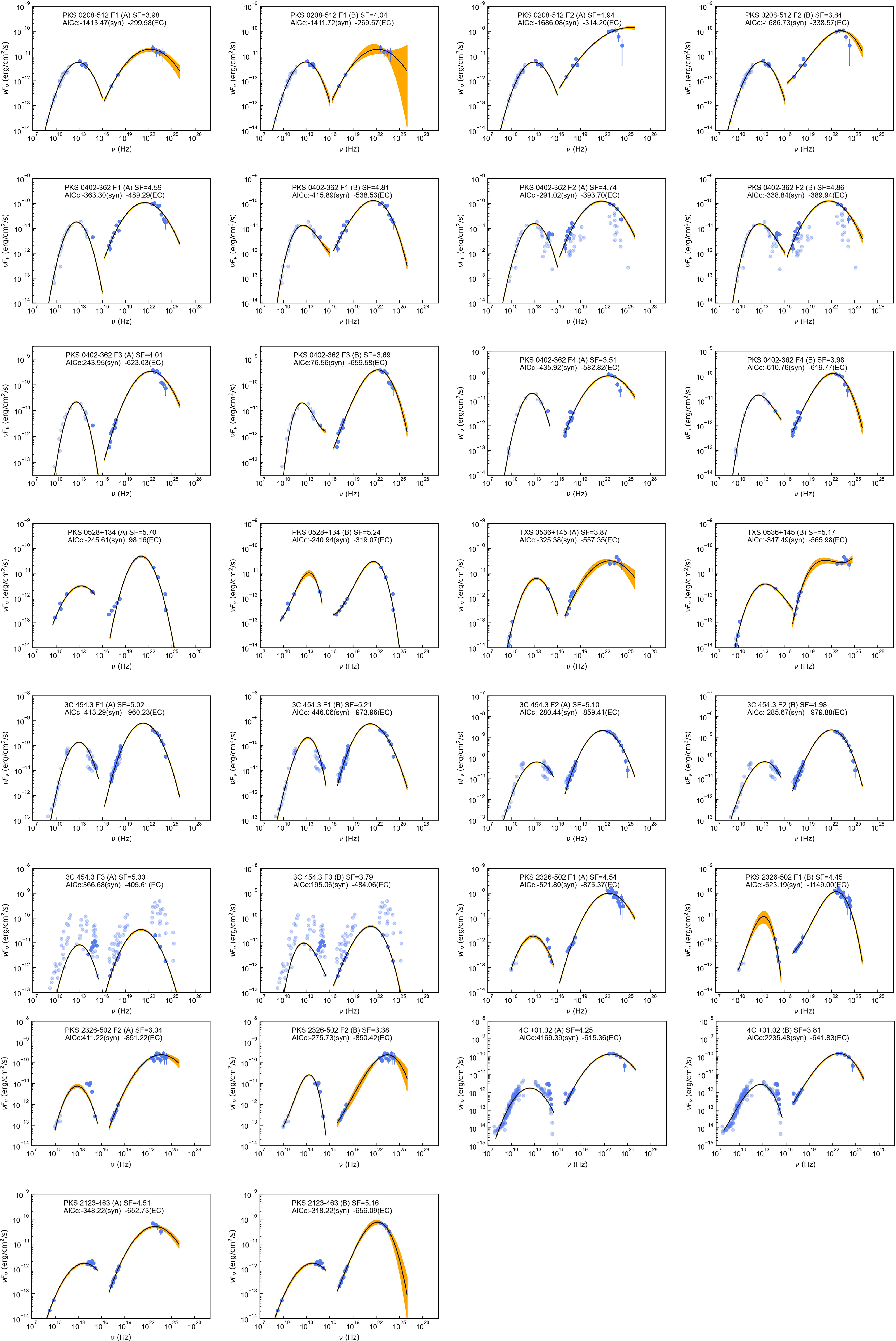
Figure A2. SED fitting results of the blazars dominated by dusty torus with variability timescales.
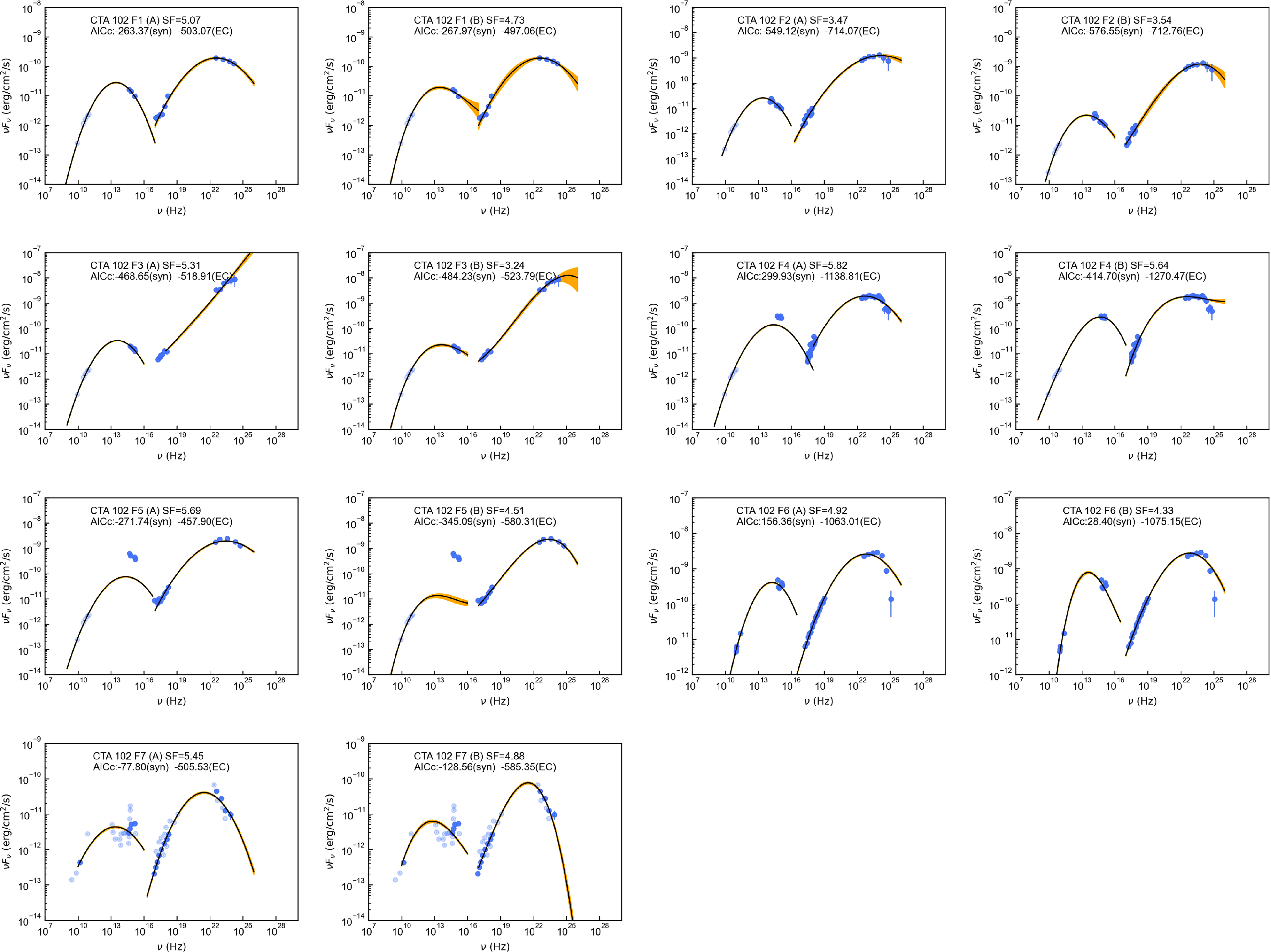
Figure A3. SED fitting results of CTA 102.
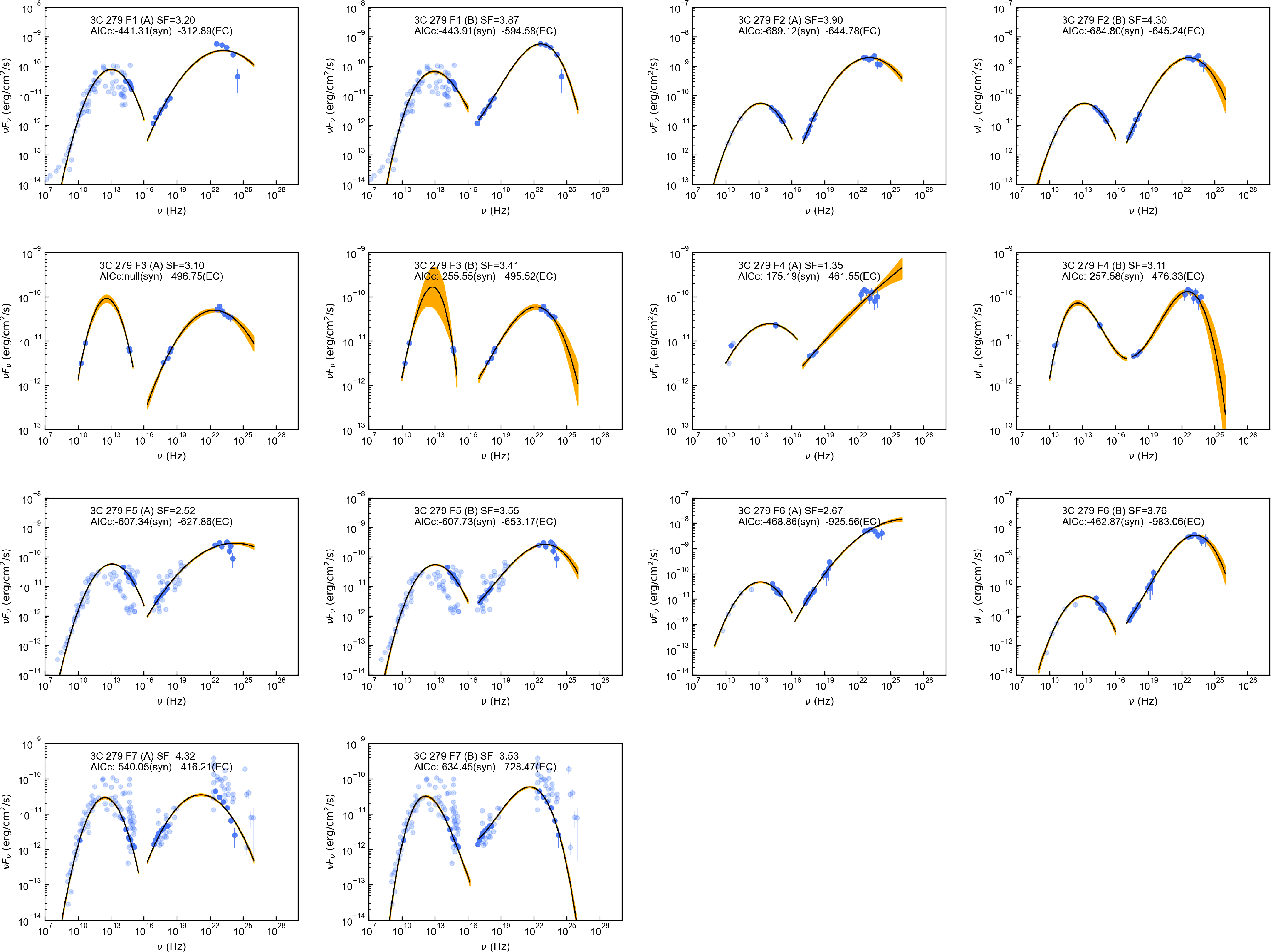
Figure A4. SED fitting results of 3C 279.

Figure A5. SED fitting results of TXS 0506+056.
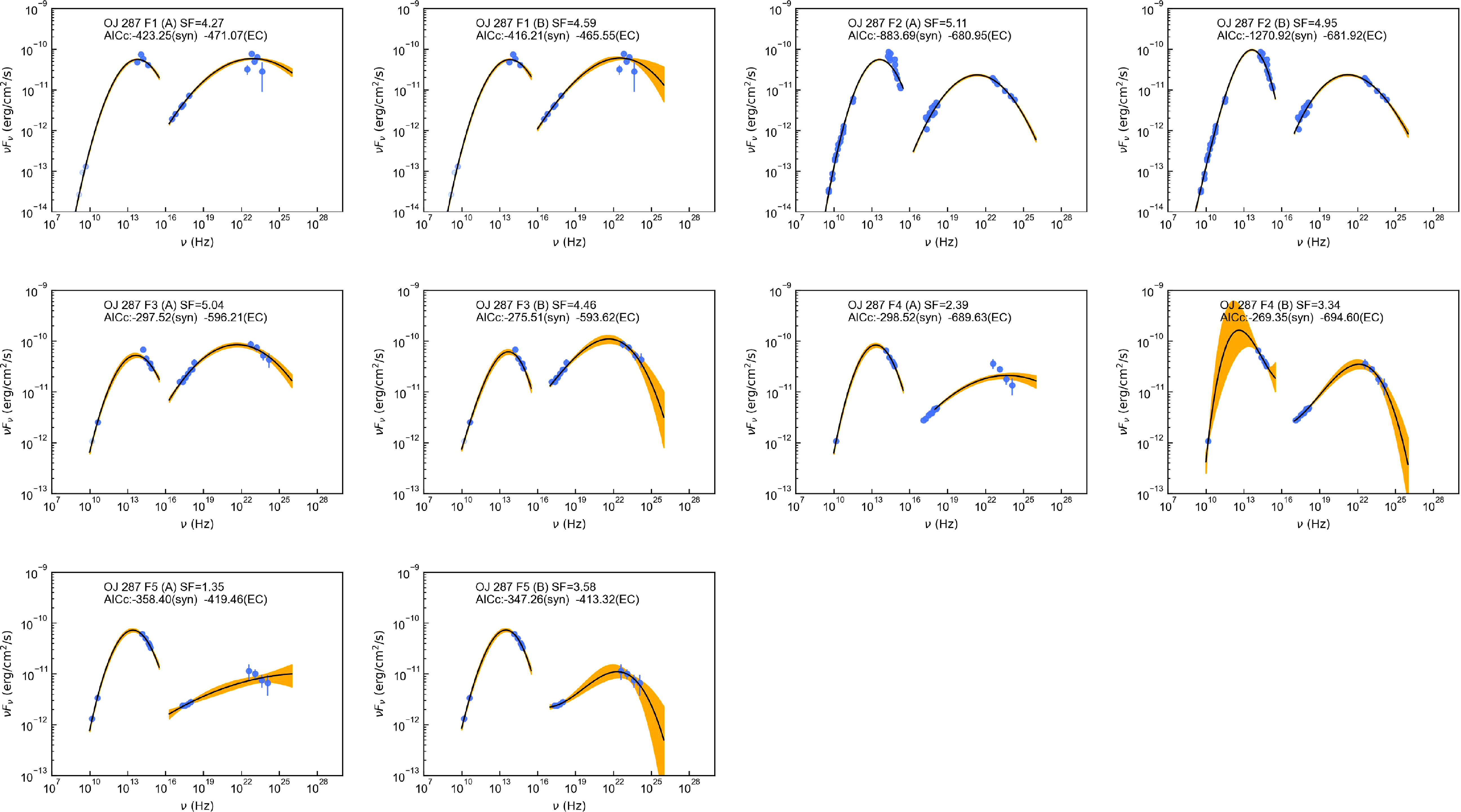
Figure A6. SED fitting results of OJ 287.


