


1. Introduction
1.1. Motivation and related literature
It is hard to find homogeneous populations in real life, as most populations of items in practice are nonhomogeneous. Heterogeneous populations in reality consist usually of a finite number of homogeneous populations. For example, populations of manufactured items in practice often have two aggregated groups, that is, the “defective” items with shorter lifetimes and “standard” items with longer, normal lifetimes [Reference Block, Savits and Wondmagegnehu11]. Heterogeneity also occurs when components manufactured at different facilities are mixed, or they are manufactured at the same facility but with changing operational or environmental characteristics, etc. [Reference Cha and Finkelstein14,Reference Finkelstein16]. Ignoring inherent heterogeneity in populations of items can lead to fundamental errors in the corresponding reliability analysis. Finite mixture models are usually an effective tool for modeling heterogeneity. Some applications of finite mixture models can be found, for example, in Everitt and Hand [Reference Everitt and Hand15].
Let  $\bar {F}(t)$ denote the survival function (SF) that describes the lifetime of an ordinary (arithmetic) finite mixture of
  $n$ homogeneous subpopulations with the SF's
  $\bar {F}_{i}(t)$,
  $i =1,\ldots,n$. Then,
 \begin{equation} \bar{F}(t)=\sum_{i=1}^{n} p_{i} \bar{F}_{i}(t), \end{equation}
where  $p_{i}$ is the mixing proportion such that
  $\sum _{i=1}^{n} p_{i}=1$ and
  $p_{i} \geq 0$, for
  $i \in \{1,2, \ldots, n\}$.
Many authors have explored various aspects of mixture models. For instance, the tail behavior of the corresponding failure rates in mixture models has been investigated by Block et al. [Reference Block, Mi and Savits10] and Block and Joe [Reference Block and Joe9]. The preservation of relevant stochastic properties for mixtures has been examined by Block et al. [Reference Block, Li and Savits12]. Block et al. [Reference Block, Savits and Wondmagegnehu11] also have studied mixtures with increasing linear failure rates. Badia et al. [Reference Badia, Berrade, Campos and Navascues5] have provided bounds for the failure rate, the failure rate average, the mean residual life and their derivatives. The relevant aging properties of the additive and proportional (multiplicative) hazards mixing models have been investigated by Badia et al. [Reference Badia, Berrade and Campos6]. Aging properties for the multivariate proportional hazards in mixtures as well as relevant stochastic comparisons have been studied by Badia and Lee [Reference Badia and Lee4]. The likelihood ratio ordering in the mixture models using Glaser's function has been investigated by Navarro [Reference Navarro24]. Stochastic comparisons for general mixtures in the sense of the hazard rate order and the likelihood ratio order have been studied by Navarro [Reference Navarro25]. Navarro and Aguila [Reference Navarro and del Aguila26] have obtained the necessary and sufficient conditions to compare two finite mixture models in the sense of the usual stochastic order and the hazard rate order. Stochastic comparisons for two finite mixture models with different baseline random variables and different mixing proportions have been studied by Amini and Zhang [Reference Amini-Seresht and Zhang2].
Hazra and Finkelstein [Reference Hazra and Finkelstein19], using the multivariate majorization, have provided a stochastic comparison for two finite mixtures when the baseline distribution belongs to some semi-parametric families of distribution such as proportional hazards, accelerated lifetimes (scale models) and proportional reversed hazards models. Stochastic comparisons for two finite mixtures using majorization in the sense of the usual stochastic order, the hazard rate order and the reversed hazard rate order have been discussed by Nadeb and Torabi [Reference Nadeb and Torabi23]. Albabtain et al. [Reference Albabtain, Shrahili, Al-Shehri and Kayid1] have considered a parametric family of weighted distributions and their mixtures and have provided some stochastic comparisons. For some aging properties and stochastic comparisons of mixtures, we refer, among others, to Finkelstein and Esaulova [Reference Finkelstein and Esaulova17], Finkelstein and Esaulova [Reference Finkelstein and Esaulova18], Shaked and Shanthikumar [Reference Shaked and Shanthikumar27] and Misra and Naqvi [Reference Misra and Naqvi22].
Recently, Asadi et al. [Reference Asadi, Ebrahimi and Soofi3] have proposed a flexible mixture model; the, so-called,  $\alpha$-mixture model that combines two popular in applications mixture models, that is, the ordinary (arithmetic) mixture model and the mixture of failure rates model. In accordance with this paper, the finite
  $\alpha$-mixture for
  $n$ subpopulations with the corresponding SF's
  $\bar {F}_{i}$,
  $i=1,2,\ldots,n$, is defined as
 \begin{equation} \bar{F}_{\alpha}(t)=\left\{ \begin{array}{ll} \displaystyle \left[ \sum_{i=1}^{n} p_{i}{\bar{F}_{i}}^{\alpha}(t) \right]^{1/\alpha}, & {\alpha \neq 0}, \\ \displaystyle \prod_{i=1}^{n}{\bar{F}_{i}}^{p_{i}}(t), & \alpha =0, \end{array} \right. \end{equation}
where  $p_{i}$ is the mixing proportion such that
  $p_{i}\geq 0$, for
  $i= 1, \ldots, n$ and
  $\sum _{i=1}^{n} p_{i}=1$. Thus Eq. (2), for
  $\alpha =1$ reduces to the arithmetic (ordinary) mixture of survival functions, whereas the case
  $\alpha \rightarrow 0$, as shown by Asadi et al. [Reference Asadi, Ebrahimi and Soofi3], defines the mixture of the failure rates (the geometric mixture of the corresponding SF's). Asadi et al. [Reference Asadi, Ebrahimi and Soofi3] have extended the classical result of Barlow and Proschan [Reference Barlow and Proschan7] on DFR (DFRA) distributions in
  $\alpha$-mixtures, stating that the
  $\alpha$-mixture of DFR (IFR) distributions are DFR (IFR) for
  $\alpha >0$ (
 $\alpha <0$) (see Section 1.2 for definitions of these notions of aging). They, also, have shown that this closure property holds for DFRA (IFRA) distributions for
  $\alpha >0$ (
 $\alpha <0$). Shojaee et al. [Reference Shojaee, Asadi and Finkelstein28] have considered the
  $\alpha$-mixture model and provided a new interpretation for the
  $\alpha$-mixture model via the multiplicative–additive hazard transform.
An obvious shortcoming of the model in Eq. (2) is that the parameter  $\alpha$ is the same for all survival functions, whereas the weights are different. For instance, the impact of the environment on different components of a multi-component system can be also different. Obviously, Eq. (2) is the specific case of a more general and practically sound in various applications and settings model with different parameters (see our discussion and examples in the beginning of the next section). Therefore, in the current study, motivated by Asadi et al. [Reference Asadi, Ebrahimi and Soofi3], we generalize some results of this paper on the finite
  $\alpha$-mixture model (e.g., relevant stochastic comparisons and aging properties) to the case with different parameters. We also discuss in detail the limiting behavior of resulting distributions, conditional characteristics and relevant stochastic ordering using majorization technique. The latter is the main focus of the second part of the paper, where some new approaches are developed and discussed using relevant examples and counterexamples.
1.2. Notation
For two random variables  $X$ and
  $Y$, we denote by
  $f$ and
  $g$, the probability density functions, by
  $F$ and
  $G$, the cumulative distribution functions, by
  $\bar {F}$ and
  $\bar {G}$, the survival functions and by
  $r_{X}$ and
  $r_{Y}$, the hazard (failure) rate functions, respectively. In this study, we will use the following concepts of aging and definitions of stochastic orders:
• The random variable
 $X$ (or its distribution $F$) is said to be an increasing (decreasing) failure rate (IFR (DFR)) if its failure rate $r_X(t)$ is nondecreasing (nonincreasing) in $t$.
• The random variable
$X$ (or its distribution $F$) is said to be an increasing (decreasing) failure rate average (IFRA (DFRA)) if $-\frac {1}{t}\log \bar {F}(t)$ is nondecreasing (nonincreasing) in $t$.• The random variable
$X$ is said to be smaller than $Y$ in the usual stochastic order (denoted by $X\leq _{\rm st}Y$ or $F\leq _{\rm st} G$) if $\bar {F}(t)\leq \bar {G}(t)$ for all $t$.• The random variable
$X$ is said to be smaller than $Y$ in the hazard rate order (denoted by $X\leq _{\rm hr}Y$ or $F\leq _{\rm hr}G$) if $\bar {G}(t)/\bar {F}(t)$ is increasing in $t$, for all $t$ or equivalently $r_X(t)\geq r_Y(t)$, for all $t$.• The random variable
$X$ is said to be smaller than $Y$ in the likelihood ratio order (denoted by $X\leq _{\rm lr}Y$ or $F\leq _{\rm lr}G$) if $g(t)/f(t)$ is increasing in $t$, for all $t$.


1.3. Organization of the paper
The organization of the paper is as follows. Section 2 defines the generalized finite  $\alpha$-mixture model and discusses its relation to other models reported in the literature. Section 3 studies the aging properties of the generalized finite
  $\alpha$-mixture. Section 4 is devoted to the special cases of additive and multiplicative models for the baseline distributions in the generalized finite
  $\alpha$-mixture. Section 5 provides some stochastic comparisons in the usual stochastic order and the hazard rate order with different baseline distributions. Section 6 provides sufficient conditions based on the concept of majorization for stochastic comparison of two generalized finite
  $\alpha$-mixtures. Finally, Section 7 gives some concluding remarks.
2. The generalized finite $\alpha$-mixture model

The generalized finite  $\alpha$-mixture of
  $n$ subpopulations with SF's
  $\bar {F}_{i}$,
  $i=1,2,\ldots,n$, is defined as
 \begin{equation} \bar{F}(t,\bar{\alpha})=\left[ \sum_{i=1}^{n} p_{i}{\bar{F}_{i}}^{\alpha_i}(t) \right]^{1/\bar{\alpha}},\quad \alpha_i\in (-\infty,\infty), \end{equation}
where  $p_{i}$ is the mixing proportion such that
  $p_{i}\geq 0$, for
  $i \in \{ 1, 2,\ldots, n\}$, and
  $\sum _{i=1}^{n} p_{i}=1$ and
  $\bar {\alpha }=\sum _{i=1}^{n}p_i\alpha _i$. Assuming that
  $\boldsymbol {p}=(p_{1},\ldots, p_{n})$ is given, it includes the following special cases:
•
$\alpha _i=1$, $i=1,\ldots,n$, give the arithmetic mixture of $\bar {F}_i$'s.•
$\alpha _i=-1$, $i=1,\ldots,n$, give the harmonic mixture of $\bar {F}_i$'s.• If
$\alpha _i=0$, $i=1,\ldots,n$, we arrive at the geometric mixture of $\bar {F}_i$'s.•
$\alpha _i=\alpha$, $i=1,\ldots,n$, give the $\alpha$-mixture of survival function.


2.1. Motivating example
Assume that we have a mixed population with two subpopulations. Let the survival functions of items in each subpopulations in laboratory conditions be denoted as  $\bar {F}_{i}(t)$,
  $i=1,2$. Suppose that the corresponding mixing proportions are
  $p$ and
  $(1-p)$, respectively. Assume that the severe conditions act on each subpopulation so that the survival functions of
  $i$th subpopulation, in accordance with the proportional hazards model, becomes
  $\bar {F}_{i}^{\alpha _i}(t)$, where
  $\alpha _i>0$,
  $i=1,2$. Then, the survival function of a randomly selected item is
 $$\bar{F}_{s}(t,\boldsymbol{\alpha})=p\bar{F}_{1}^{\alpha_1}(t)+(1-p)\bar{F}_{2}^{\alpha_2}(t).$$
Assume now that an item is shielded from the severe conditions. However, this shielding is “executed” also by the proportional hazards model that decreases proportionally the failure rate that corresponds to the foregoing survival function. Thus, as it can be clearly seen, by this operation, we cannot arrive exactly at the initial mixed survival function (in laboratory conditions). Since the severe conditions parameter of the first selected item is  $\alpha _1$ with probability
  $p$, and that of the second item is
  $\alpha _2$ with probability
  $(1-p)$, we consider the average value of the parameter in accordance with which the selected item is shielded, that is,
  $p\alpha _1+(1-p)\alpha _2$. Hence, the survival function of the selected component after these operations is
 $$\bar{F}(t,\bar{\alpha})=(p\bar{F}_{1}^{\alpha_1}(t)+(1-p)\bar{F}_{2}^{\alpha_2}(t))^{{1}/{\bar{\alpha}}},$$
where  $\bar {\alpha }=p\alpha _1+(1-p)\alpha _2$.
2.2. Relation to models in the literature
In what follows, we interpret some of the existent in the literature specific models in terms of the generalized finite  $\alpha$-mixtures. Note that the subpopulations/populations of items are considered as sufficiently large. Cha [Reference Cha13] has considered the following two selection policies for designing the
  $m$-component series system:
• The
$m$-component series systems are built only using one type of component. Assume that the proportion of systems built using the $i$th component with the SF $\bar {F}_{i}(t)$, $i=1,\ldots,n$, is $p_{i}$, $i=1,\ldots,n$. A system is randomly selected from the large mixed set of systems. This model is defined as “mixing at the system level.” The SF of the selected series system is
where$$\mathcal{\bar{F}}_{1}(t)=\sum_{i=1}^{n} p_{i} \bar{F}^{m}_{i}(t)=\bar{F}^{m}(t,m),\nonumber$$
$\bar {F}(t,m)$, as the $m$th root of the sum above, according to our definition, is the SF of the generalized finite $\alpha$-mixture with $\alpha _{i}=m$, $i=1, \ldots, n$. Let $\bar {F}_{i}(t)$ belong to the proportional hazard model, $\bar {F}_{i}(t)=\bar {G}^{r_{i}}_{i}(t)$ and set $m r_{i}=\alpha _{i}$, $i=1, \ldots, n$. Thus,
where$$\mathcal{\bar{F}}_{1}(t)=\sum_{i=1}^{n} p_{i} \bar{G}^{\alpha_{i}}_{i}(t)=\bar{G}^{ \bar{\alpha}}(t,\bar{\alpha})=\bar{G}^{m \bar{r}}(t,m\bar{r}),$$
$\bar {G}(t,\bar {\alpha })$ is the SF of the generalized finite $\alpha$-mixture corresponding to $\bar {G}_{i}$, $i=1, \ldots, n$, and $\bar {r}=\sum _{i=1}^{n} p_{i} r_{i}$.• The system is “built randomly” using
$n$ types of components. If the proportion of the $i$th component with the SF $\bar {F}_{i}(t)$ is $p_{i}$, $i=1,\ldots, n$, then the SF of the built series system of m components is:
where$$\mathcal{\bar{F}}_{2}(t)=\left( \sum_{i=1}^{n} p_{i} \bar{F}_{i}(t)\right)^{m}=\bar{F}^{m}(t,1),$$
$\bar {F}(t,1)$ is the SF of the generalized finite $\alpha$-mixture with $\alpha _{i}=1$, $i=1, \ldots, n$. This model can be called “mixing at the component level.” Let $\bar {F}_{i}(t)$ belong to the proportional hazard model, $\bar {F}_{i}(t)=\bar {G}^{\alpha _{i}}_{i}(t)$, $i=1, \ldots, n$. Thus,
where$$\mathcal{\bar{F}}_{2}(t)=\left( \sum_{i=1}^{n} p_{i} \bar{G}^{\alpha_{i}}_{i}(t) \right)^{m}=(\bar{G}^{\bar{\alpha}}(t,\bar{\alpha}))^{m},$$
$\bar {G}(t,\bar {\alpha })$ is the SF of the generalized finite $\alpha$-mixture corresponding to $\bar {G}_{i}$, $i=1, \ldots, n$, and $\bar {\alpha }=\sum _{i=1}^{n} p_{i} \alpha _{i}$.


For generalizations of these two models, see Hazra et al. [Reference Hazra, Finkelstein and Cha20].
3. Hazard rate and aging properties of the generalized finite $\alpha$-mixture

The generalized finite  $\alpha$-mixture of SF's
  $\bar {F}_{i}$ for
  $i=1,2,..,n$, in accordance with our definition, is
 $$\bar{F}(t,\bar{\alpha})=\left[ \sum_{i=1}^{n} p_{i}{\bar{F}_{i}}^{\alpha_i}(t) \right]^{1/\bar{\alpha}},\quad \alpha_i\in (-\infty,\infty).$$
Then, the corresponding PDF is
 $$f(t,\bar{\alpha})=\frac{1}{\bar{\alpha}}\left[ \sum_{i=1}^{n} \alpha_{i} p_{i}f_{i}(t){\bar{F}_{i}}^{\alpha_{i}-1}(t) \right] \left[ \sum_{i=1}^{n} p_{i}{\bar{F}_{i}}^{\alpha_{i}}(t) \right]^{\frac{1}{\bar{\alpha}}-1},$$
where  $p_{i}$ is the mixing proportion such that
  $\sum _{i=1}^{n} p_{i}=1$ and
  $p_{i}\geq 0$, for
  $i \in \{ 1, 2,\ldots, n\}$ and
  $\bar {\alpha }=\sum _{i=1}^{n}p_i\alpha _i$.
If  $r(t,\bar {\alpha })$ and
  $r_{i}(t)$ denote, respectively, the hazard rate of the generalized finite
  $\alpha$-mixture and the hazard rate of the
  $i$th component, then
 \begin{align} r(t,\bar{\alpha})& =\frac{f(t,\bar{\alpha})}{\bar{F}(t,\bar{\alpha})} \nonumber\\ & =\frac{1}{\bar{\alpha}} \frac{ \sum_{i=1}^{n} \alpha_{i} p_{i}r_{i}(t){\bar{F}_{i}}^{\alpha_{i}}(t)}{\sum_{j=1}^{n} p_{j}{\bar{F}_{j}}^{\alpha_{j}}(t)} \nonumber\\ & =\frac{1}{\bar{\alpha}}\sum_{i=1}^{n} \alpha_{i} r_{i}(t) p_{\alpha_{i}}(t), \end{align}
where  $p_{\alpha _{i}}(t)={p_{i} \bar {F}_{i}^{\alpha _{i}}(t)}/{\sum _{j=1}^{n} p_{j} \bar {F}_{j}^{\alpha _{j}}(t)}$.
As an example, let us consider first, a mixture of two SFs  $\bar {F}_{1}(t)$ and
  $\bar {F}_{2}(t)$ with PDFs
  $f_{1}(t)$ and
  $f_{2}(t)$ and hazard rates
  $r_{1}(t)$ and
  $r_{2}(t)$, respectively. We are interested in the bounds for the mixture hazard rate that is defined in this case as
 \begin{align*} r(t,\bar{\alpha})& =\frac{1}{\bar{\alpha}} \left[ \alpha_{1} r_{1}(t) \frac{ p{\bar{F}_{1}}^{\alpha_{1}}(t)}{ p{\bar{F}_{1}}^{\alpha_{1}}(t)+ (1-p){\bar{F}_{2}}^{\alpha_{2}}(t)}+\alpha_{2} r_{2}(t) \frac{ (1-p){\bar{F}_{2}}^{\alpha_{2}}(t)}{ p{\bar{F}_{1}}^{\alpha_{1}}(t)+ (1-p){\bar{F}_{2}}^{\alpha_{2}}(t)}\right] \nonumber\\ & =\frac{1}{\bar{\alpha}} [ \alpha_{1} r_{1}(t) p_{\alpha}(t) +\alpha_{2} r_{2}(t) (1-p_{\alpha}(t))], \nonumber \end{align*}
where the time-dependent probabilities are
 $$p_{\alpha}(t)=\frac{ p{\bar{F}_{1}}^{\alpha_{1}}(t)}{ p{\bar{F}_{1}}^{\alpha_{1}}(t)+ (1-p){\bar{F}_{2}}^{\alpha_{2}}(t)}, \quad (1-p_{\alpha}(t))=\frac{ (1-p){\bar{F}_{2}}^{\alpha_{2}}(t)}{ p{\bar{F}_{1}}^{\alpha_{1}}(t)+ (1-p){\bar{F}_{2}}^{\alpha_{2}}(t)}.$$
From this representation, we have [Reference Finkelstein16]:
 $$\min\left\{\frac{\alpha_{1}}{\bar{\alpha}}r_{1}(t), \frac{\alpha_{2}}{\bar{\alpha}}r_{2}(t)\right\} \leq r(t,\bar{\alpha}) \leq \max\left\{\frac{\alpha_{1}}{\bar{\alpha}}r_{1}(t), \frac{\alpha_{2}}{\bar{\alpha}}r_{2}(t) \right\}.$$
In particular for  $\alpha _{i} > 0$, if
  $\alpha _{1} \leq \alpha _{2}$ and
  $F_{1} \geq _{\rm hr} F_{2}$, then
 $$\frac{\alpha_{1}}{\bar{\alpha}}r_{1}(t) \leq r(t,\bar{\alpha}) \leq \frac{\alpha_{2}}{\bar{\alpha}}r_{2}(t),$$
and for  $\alpha _{i} < 0$, if
  $\alpha _{1} \leq \alpha _{2}$ and
  $F_{1} \leq _{\rm hr} F_{2}$, then
 $$\frac{\alpha_{2}}{\bar{\alpha}}r_{2}(t) \leq r(t,\bar{\alpha}) \leq \frac{\alpha_{1}}{\bar{\alpha}}r_{1}(t).$$
Generalizing the foregoing result, in the following theorem, we show that the lifetimes in the weakest (strongest) subpopulation is smaller (greater) than that of the generalized finite  $\alpha$-mixture of
  $n$ subpopulations in the sense of the hazard rate order for
  $\alpha _{i} > 0$ (
 $\alpha _{i} < 0$),
  $i=1,2, \ldots, n$.
Theorem 3.1 Let the lifetimes in subpopulations be ordered in the sense of the hazard rate ordering, that is,  $F_{1} \leq _{hr} F_{2} \leq _{hr} \cdots \leq _{hr} F_{n}$. Then, for all
  $t$,
$t$,
 $${F_{1}\leq_{hr} F(t,\bar{\alpha}),}$$
for all ordered  $\alpha _{i}>0$,
  $i=1,\ldots, n$, whereas for all ordered
  $\alpha _{i}<0$,
  $i=1,\ldots, n$:
 $$F(t,\bar{\alpha}) \leq_{hr} F_{n}.$$
Proof. We only give proof for  $\alpha _{i}>0$,
  $i=1,\ldots, n$ because the proof for
  $\alpha _{i}<0$,
  $i=1,\ldots, n$ is completely similar. Let
  $\alpha _{i}>0$,
  $i=1,\ldots, n$. We need to show that
  $r(t,\bar {\alpha })-r_{1}(t)\leq 0$ for all
  $t$. We have
 \begin{align*} r(t,\bar{\alpha})-r_{1}(t)& =\frac{1}{\bar{\alpha}(\sum_{i=1}^{n} p_{i}\bar{F}^{\alpha_{i}}_{i}(t))}\left( \sum_{i=1}^{n} r_{i}(t) \alpha_{i}p_{i}\bar{F}^{\alpha_{i}}_{i}(t)\right) - r_{1}(t)\\ & =\dfrac{( \sum_{i=1}^{n} r_{i}(t) \alpha_{i}p_{i}\bar{F}^{\alpha_{i}}_{i}(t))-( (\sum_{i=1}^{n} \alpha_{i}p_{i})(\sum_{i=1}^{n} p_{i}\bar{F}^{\alpha_{i}}_{i}(t)) )r_{1}(t)}{\bar{\alpha}(\sum_{i=1}^{n} p_{i}\bar{F}^{\alpha_{i}}_{i}(t))}\\ & \stackrel{\textrm{sign}}{=}\left( \sum_{i=1}^{n} r_{i}(t) \alpha_{i}p_{i}\bar{F}^{\alpha_{i}}_{i}(t)\right)-\left( \left(\sum_{i=1}^{n} \alpha_{i}p_{i}\right)\left(\sum_{i=1}^{n} p_{i}\bar{F}^{\alpha_{i}}_{i}(t)\right) \right)r_{1}(t). \end{align*}
From the assumption  $F_{1} \leq _{hr} F_{2} \leq _{hr} \cdots \leq _{hr} F_{n}$, we have
  $r_{1}(t) \geq \cdots \geq r_{n}(t)$. This implies that
 \begin{align*} & \left( \sum_{i=1}^{n} r_{i}(t) \alpha_{i}p_{i}\bar{F}^{\alpha_{i}}_{i}(t)\right)-\left( \left(\sum_{i=1}^{n} \alpha_{i}p_{i}\right)\left(\sum_{i=1}^{n} p_{i}\bar{F}^{\alpha_{i}}_{i}(t)\right) \right)r_{1}(t)\\ & \quad \leq r_{1}(t) \left( \sum_{i=1}^{n} \alpha_{i}p_{i}\bar{F}^{\alpha_{i}}_{i}(t)\right)-\left( \left(\sum_{i=1}^{n} \alpha_{i}p_{i}\right)\left(\sum_{i=1}^{n} p_{i}\bar{F}^{\alpha_{i}}_{i}(t)\right) \right)r_{1}(t). \end{align*}
Thus,
 \begin{align*} r(t,\bar{\alpha})-r_{1}(t)& \stackrel{\textrm{sign}}{=} r_{1}(t) \left[ \alpha_{1}p_{1}(1-p_{1})\bar{F}^{\alpha_{1}}_{1}(t)+\alpha_{2}p_{2}(1-p_{2})\bar{F}^{\alpha_{2}}_{2}(t)+\cdots + \alpha_{n}p_{n}(1-p_{n})\bar{F}^{\alpha_{n}}_{n}(t)\vphantom{\sum_{j\neq 1}^{n}}\right.\\ & \quad \left.-\alpha_{1}p_{1} \sum_{j\neq 1}^{n} p_{j} \bar{F}^{\alpha_{j}}_{j}(t)-\alpha_{2}p_{2} \sum_{j\neq 2}^{n} p_{j} \bar{F}^{\alpha_{j}}_{j}(t)-\cdots -\alpha_{n}p_{n} \sum_{j\neq n}^{n} p_{j} \bar{F}^{\alpha_{j}}_{j}(t) \right]\\ & =r_{1}(t)\left[\sum_{i=1}^{n} \alpha_{i}p_{i}(1-p_{i})\bar{F}^{\alpha_{i}}_{i}(t)-\sum_{i=1}^{n} \alpha_{i}p_{i} \sum_{j \neq i}^{n} p_{j} \bar{F}^{\alpha_{j}}_{j}(t) \right]\\ & =r_{1}(t)\left[\sum_{i=1}^{n} \alpha_{i}p_{i} \left( \sum_{j \neq i}^{n} p_{j}\bar{F}^{\alpha_{i}}_{i}(t)-\sum_{j \neq i}^{n} p_{j} \bar{F}^{\alpha_{j}}_{j}(t)\right) \right]\\ & =r_{1}(t)\left[\sum_{i=1}^{n} \alpha_{i}p_{i} \left( \sum_{j \neq i}^{n} p_{j}(\bar{F}^{\alpha_{i}}_{i}(t)- \bar{F}^{\alpha_{j}}_{j}(t))\right) \right]\\ & =r_{1}(t)\left[\sum_{i=2}^{n} p_{1} p_{i} (\bar{F}^{\alpha_{1}}_{1}(t)- \bar{F}^{\alpha_{i}}_{i}(t))(\alpha_{1}-\alpha_{i})\right.\\ & \quad + \sum_{i=3}^{n} p_{2} p_{i} (\bar{F}^{\alpha_{2}}_{2}(t)- \bar{F}^{\alpha_{i}}_{i}(t))(\alpha_{2}-\alpha_{i})+ \cdots\\ & \quad \left.\vphantom{\sum_{i=3}^{n}} + p_{n-1} p_{n} (\bar{F}^{\alpha_{n-1}}_{n-1}(t)- \bar{F}^{\alpha_{n}}_{n}(t))(\alpha_{n-1}-\alpha_{n})\right]\\ & \leq r_{1}(t)\left[\sum_{i=2}^{n} p_{1} p_{i} (\bar{F}^{\alpha_{1}}_{1}(t)- \bar{F}^{\alpha_{i}}_{1}(t))(\alpha_{1}-\alpha_{i})\right.\\ & \quad + \sum_{i=3}^{n} p_{2} p_{i} (\bar{F}^{\alpha_{2}}_{2}(t)- \bar{F}^{\alpha_{i}}_{2}(t))(\alpha_{2}-\alpha_{i})+ \cdots\\ & \quad \left.\vphantom{\sum_{i=2}^{n}}+ p_{n-1} p_{n} (\bar{F}^{\alpha_{n-1}}_{n-1}(t)- \bar{F}^{\alpha_{n}}_{n-1}(t))(\alpha_{n-1}-\alpha_{n})\right]. \end{align*}
As the hazard rate order implies the usual stochastic order, the assumption  $F_{1} \leq _{hr} F_{2} \leq _{hr} \cdots \leq _{hr} F_{n}$ yields
  $\bar {F}_{1}(t) \leq \bar {F}_{2}(t) \leq \cdots \leq \bar {F}_{n}(t)$. Thus,
  $\bar {F}^{\alpha _{j}}_{i}(t) \leq \bar {F}^{\alpha _{j}}_{j}(t)$ for
  $i \leq j$,
  $i,j=1,2,\ldots, n$, and then
  $(\bar {F}^{\alpha _{i}}_{i}(t)-\bar {F}^{\alpha _{j}}_{j}(t)) \leq (\bar {F}^{\alpha _{i}}_{i}(t)-\bar {F}^{\alpha _{j}}_{i}(t))$ and last inequality holds.
Consider now the following two cases for  $\alpha _{i} > 0$ separately.
• Let
$\alpha _{1} \geq \alpha _{2} \geq \cdots \geq \alpha _{n}$. In this case $\bar {F}^{\alpha _{i}}_{i}(t)\leq \bar {F}^{\alpha _{j}}_{i}(t)$ for $i \leq j$, $i,j=1,2,\ldots, n$ and then $(\bar {F}^{\alpha _{i}}_{i}(t)- \bar {F}^{\alpha _{j}}_{i}(t))\leq 0$. Since $( \alpha _{i}-\alpha _{j})\geq 0$ for $i \leq j$, $i,j=1,2,\ldots, n$, thus
$$r(t,\bar{\alpha})-r_{1}(t) \leq 0.$$
• Let
$\alpha _{1} \leq \alpha _{2} \leq \cdots \leq \alpha _{n}$. In this case $\bar {F}^{\alpha _{i}}_{i}(t)\geq \bar {F}^{\alpha _{j}}_{i}(t)$ for $i \leq j$, $i,j=1,2,\ldots, n$ and then $(\bar {F}^{\alpha _{i}}_{i}(t)- \bar {F}^{\alpha _{j}}_{i}(t))\geq 0$. Since $( \alpha _{i}-\alpha _{j})\leq 0$ for $i \leq j$, $i,j=1,2,\ldots, n$, thus
$$r(t,\bar{\alpha})-r_{1}(t) \leq 0.$$


Thus, in general,  $r(t,\bar {\alpha })-r_{1}(t)\leq 0$, which means that
  $F_{1}\leq _{hr} F(t, \bar {\alpha })$ for
  $\alpha _{i}>0$,
  $i=1,\ldots, n$. This completes the proof.
In the following, we study the closure property of the generalized finite  $\alpha$-mixture. For proving the main result, we first provide the following definition and lemma.
Definition 3.1 The hazard transform of the generalized finite  $\alpha$-mixture is
 \begin{equation} \eta_{\bar{\alpha}}(\textbf{u})={-}\frac{1}{\bar{\alpha}} \log\left(\sum_{i=1}^{n} p_{i} e^{-\alpha_{i}u_{i}}\right), \quad \alpha_i\in (-\infty,\infty), \end{equation}
where  $\textbf {u}$ is a vector with elements
  $u_{i}$,
  $0 \leq u_{i}\leq \infty$.
Thus, the hazard function  $R(t,\bar {\alpha })=\int _{0}^{u} r(u,\bar {\alpha }) \,du$ that corresponds to the lifetime described by the generalized finite
  $\alpha$-mixture is given by
 \begin{equation} R(t,\bar{\alpha})=\eta_{\bar{\alpha}}(\textbf{R}(t))\equiv{-}\frac{1}{\bar{\alpha}} \log\left(\sum_{i=1}^{n} p_{i} e^{-\alpha_{i}R_{i}(t)}\right), \quad 0\leq t<\infty, \end{equation}
where  $R_{i}(t)=\int _{0}^{u} r_{i}(u) du$,
  $i=1,\ldots,n$ is the hazard function that corresponds to
  $\bar {F}_{i}(t)$ and
  $\textbf {R}(t)$ is a vector.
Now we can prove the following lemma, which is an extension of Lemma A.1 of Asadi et al. [Reference Asadi, Ebrahimi and Soofi3].
Lemma 3.1 The hazard transform  $\eta _{\bar {\alpha }}(\textbf {u})$ of the generalized finite
  $\alpha$-mixture is concave for
  $\alpha _{i}>0$ and convex for
  $\alpha _{i}<0$. That is, for
  $\alpha _{i}>0$ (
 $\alpha _{i}<0$)
 \begin{equation} \eta_{\bar{\alpha}}(\beta\textbf{u}+(1-\beta)\textbf{v})\geq ({\leq}) \beta \eta_{\bar{\alpha}}(\textbf{u})+(1-\beta)\eta_{\bar{\alpha}}(\textbf{v}), \end{equation}
where  $0\leq \beta \leq 1$ and
  $0 \leq u_{i},v_{i}\leq \infty$ for
  $i=1,..,n$.
Proof. Using Holder's inequality, we have (for  $\alpha _{i}>0$ (
 $\alpha _{i}<0$)):
 $$\sum_{i=1}^{n} p_{i} \,e^{-\beta \alpha_{i}u_{i}}\, e^{-(1-\beta) \alpha_{i}v_{i}} \leq \left( \sum_{i=1}^{n} p_{i} \,e^{- \alpha_{i}u_{i}} \right) ^{\beta} \left( \sum_{i=1}^{n} p_{i}\, e^{- \alpha_{i}v_{i}} \right) ^{(1-\beta)}.$$
Thus, the lemma follows the definition of  $\eta _{\bar {\alpha }}$.
In order to prove the corresponding closure theorem, we need also the following lemma from Barlow and Proschan [Reference Barlow and Proschan7].
Lemma 3.2 If  $h(u)$ is a concave (convex) function and is increasing in each argument and if
  $u(t)$ is concave (convex), then
  $g_{u}(t) \equiv h(u(t))$ is concave (convex).
Theorem 3.2 Let  $\bar {F}(t,\bar {\alpha })$ be the generalized finite
  $\alpha$-mixture. Then,
(a) If each
$\bar {F}_{i}(t)$ is DFR (IFR), then for $\alpha _{i}>0$ $(\alpha _{i}<0)$ , $\bar {F}(t,\bar {\alpha })$ is DFR (IFR).(b) If each
$\bar {F}_{i}(t)$ is DFRA (IFRA), then for $\alpha _{i}>0$ $(\alpha _{i}<0)$ , $\bar {F}(t,\bar {\alpha })$ is DFRA (IFRA).


Proof. (a) Part (a) follows from Lemmas 3.1 and 3.2.
(b) As  $\bar {F}_{i}(t)$ is DFRA (IFRA), and
  $\eta _{\bar {\alpha }}$ is increasing, the hazard function
  $R(t,\bar {\alpha })$ of the generalized finite
  $\alpha$-mixture satisfies
 $$\eta_{\bar{\alpha}}(\textbf{R}(\beta t)) \geq ({\leq}) \eta_{\bar{\alpha}}(\beta\textbf{R}(t)), \quad 0\leq \beta \leq 1.$$
Choosing  $\textbf {v} = 0$ in the result of Lemma 3.1, we obtain
 $$\eta_{\bar{\alpha}}(\beta\textbf{R}(t)) \geq ({\leq}) \beta \eta_{\bar{\alpha}}(\textbf{R}(t)).$$
Thus,
 $$R(\beta t,\bar{\alpha}) \geq ({\leq}) \beta R( t,\bar{\alpha}),$$
and hence,  $\bar {F}(t,\bar {\alpha })$ is DFRA (IFRA).
The following example provides some applications of Theorems 3.1 and 3.2.
Example 3.1 Let  $\bar {F}_{1}(t)=\exp (-0.8 t)$,
  $t>0$ and
  $\bar {F}_{2}(t)=\exp (-0.4 t)$,
  $t>0$. If we assume that
  $(p_{1},p_{2})=(0.7,0.3)$ and
  $(\alpha _{1},\alpha _{2})=(2,5)$, then clearly,
  $F_1 \leq _{hr} F_2$. Since
  $\alpha _i >0$,
  $i=1,2$, then the conditions of Theorem 3.1 are satisfied. Thus, the
  $\alpha$-mixture hazard rate in this case is equal to
 $$r(t,\bar{\alpha})=\frac{1}{2.9} \times \frac{1.12 \exp({-}1.6 t)+0.6 \exp({-}2 t)}{ \exp({-}1.6 t)+ \exp({-}2 t)}.$$
As an example of Theorem 3.1, Figure 1(a) depicts the plot of  $r(t,\bar {\alpha })$ and the hazard rate of the weakest subpopulation (
 $r_1(t)=0.8$). The plots show that,
  $F_1 \leq _{hr} F(t,\bar {\alpha })$. On the other hand, one can see that
  $\bar {F}_{1}(t)$ and
  $\bar {F}_{2}(t)$ are DFR and,
  $\bar {F}(t,\bar {\alpha })$ is also DFR for
  $\alpha _i >0$,
  $i=1,2$. As an application of Theorem 3.2, set
  $(\alpha _{1},\alpha _{2})=(-2,-5)$. Similarly, we can see from Figure 1(b) that,
  $F(t,\bar {\alpha }) \leq _{hr} F_2$ for
  $\alpha _i <0$,
  $i=1,2$. Also,
  $\bar {F}_{1}(t)$ and
  $\bar {F}_{2}(t)$ are IFR and,
  $\bar {F}(t,\bar {\alpha })$ is also IFR for
  $\alpha _i <0$,
  $i=1,2$.

Figure 1. (a) The plots of  $r(t,\bar {\alpha })$ (solid) and the hazard rate of the weakest subpopulation (dash dot) for
  $\alpha _i >0$. (b) The plots of
  $r(t,\bar {\alpha })$ (solid) and the hazard rate of the strongest subpopulation (dash dot) for
  $\alpha _i <0$.
3.1. Conditional characteristics
It is useful for further analysis in this section (see also the examples in the next section and Section 6, where we discuss stochastic comparisons using majorization technique) to rewrite some relationships (e.g., for the hazard rate functions) in a slightly different way. Then, the relevant conditional characteristics will emerge naturally. For this, first consider a non-negative discrete random variable  $\Lambda$ with probability mass
  $\pi (\lambda _{i})=p_{i}$ at
  $\lambda =\lambda _{i}$,
  $i=1,2,\ldots,n$. Also, let
  $\bar {F}(t \,|\, \lambda _{i})=\bar {F}_{i}(t)$,
  $f(t \,|\, \lambda _{i})=f_{i}(t)$ and
  $r(t \,|\, \lambda _{i})=r_{i}(t)$,
  $i=1,2,\ldots,n$. Thus, the hazard rate that corresponds to the generalized finite
  $\alpha$-mixture can be given as follows:
 \begin{align} r(t,\bar{\alpha})& =\sum_{i=1}^{n} \frac{\alpha_{i} }{\bar{\alpha}} r_{i}(t) \frac{ p_{i}{\bar{F}_{i}}^{\alpha_{i}}(t)}{\sum_{j=1}^{n} p_{j}{\bar{F}_{j}}^{\alpha_{j}}(t)}\nonumber\\ & =\sum_{i=1}^{n} \frac{\alpha_{i} }{\bar{\alpha}} r(t \,|\, \lambda_{i}) \frac{ \pi(\lambda_{i}){\bar{F}}^{\alpha_{i}}(t \,|\, \lambda_{i})}{\sum_{j=1}^{n} \pi(\lambda_{j}){\bar{F}}^{\alpha_{j}}(t \,|\, \lambda_{j})} \nonumber\\ & =\sum_{i=1}^{n} \frac{\alpha_{i} }{\bar{\alpha}} r(t \,|\, \lambda_{i}) \pi_{\bar{\alpha}}(\lambda_{i}\, |\, t), \end{align}
where
 \begin{equation} \pi_{\bar{\alpha}}(\lambda_{i}\, |\, t)=\frac{ \pi(\lambda_{i}){\bar{F}}^{\alpha_{i}}(t \,|\, \lambda_{i})}{\sum_{j=1}^{n} \pi(\lambda_{j}){\bar{F}}^{\alpha_{j}}(t \,|\, \lambda_{j})} \end{equation}
is the conditional probability mass at  $\lambda =\lambda _{i}$,
  $i=1,2,\ldots,n$ and
  $\bar {\alpha }=\sum _{i=1}^{n} \alpha _{i} \pi (\lambda _{i})$ is the weighted average of
  $\alpha _{i}$,
  $i=1,2,\ldots,n$, with weights
  $\pi (\lambda _{i})$.
Denote by  $E_{\bar {\alpha }}(\Lambda \, |\, t)$ the conditional expectation of
  $\Lambda$, that is,
 \begin{equation} E_{\bar{\alpha}}(\Lambda\, |\, t)=\sum_{i=1}^{n} \lambda_{i} \pi_{\bar{\alpha}}(\lambda_{i}\, |\, t) \end{equation}
and by  $\phi _{\bar {\alpha }}(t)$ the derivative of
  $E_{\bar {\alpha }}(\Lambda \, |\, t)$ with respect to
  $t$, that is,
 $$\phi_{\bar{\alpha}}(t)=\frac{\partial}{\partial t} E_{\bar{\alpha}}(\Lambda\, |\, t)= \sum_{i=1}^{n} \lambda_{i} \frac{\partial}{\partial t}\pi_{\bar{\alpha}}(\lambda_{i}\, |\, t),$$
where
 \begin{align*} \frac{\partial}{\partial t}\pi_{\bar{\alpha}}(\lambda_{i}\, |\, t)& =\frac{ [ -\pi(\lambda_{i}) \alpha_{i} f(t \,|\, \lambda_{i}) \bar{F}^{\alpha_{i}-1}(t \,|\, \lambda_{i})] [ \sum_{j=1}^{n} \pi(\lambda_{j}){\bar{F}}^{\alpha_{j}}(t \,|\, \lambda_{j})] } {[ \sum_{j=1}^{n} \pi(\lambda_{j}){\bar{F}}^{\alpha_{j}}(t \,|\, \lambda_{j})]^{2}}\\ & \quad +\frac{[ \sum_{j=1}^{n} \pi(\lambda_{j})\alpha_{j} f(t \,|\, \lambda_{j}){\bar{F}}^{\alpha_{j}-1}(t \,|\, \lambda_{j})] [ \pi(\lambda_{i}) \bar{F}^{\alpha_{i}}(t \,|\, \lambda_{i})] }{[ \sum_{j=1}^{n} \pi(\lambda_{j}){\bar{F}}^{\alpha_{j}}(t \,|\, \lambda_{j})]^{2}} \\ & =\frac{ [ \pi(\lambda_{i}) \bar{F}^{\alpha_{i}}(t \,|\, \lambda_{i})] [ \sum_{j=1}^{n} \alpha_{j} r(t \,|\, \lambda_{j}) \pi(\lambda_{j}) {\bar{F}}^{\alpha_{j}}(t \,|\, \lambda_{j})] }{[ \sum_{j=1}^{n} \pi(\lambda_{j}){\bar{F}}^{\alpha_{j}}(t \,|\, \lambda_{j})]^{2}}-\frac{ \alpha_{i} r(t \,|\, \lambda_{i}) \pi(\lambda_{i}) \bar{F}^{\alpha_{i}}(t \,|\, \lambda_{i})} { \sum_{j=1}^{n} \pi(\lambda_{j}){\bar{F}}^{\alpha_{j}}(t \,|\, \lambda_{j})} \\ & =\pi_{\bar{\alpha}}(\lambda_{i}\, |\, t) \bar{\alpha} r(t, \bar{\alpha})-\alpha_{i} r(t \,|\, \lambda_{i}) \pi_{\bar{\alpha}}(\lambda_{i}\, |\, t). \end{align*}
Thus,
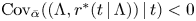
 \begin{align*} \phi_{\bar{\alpha}}(t) & =\bar{\alpha} \left[ r(t, \bar{\alpha})E_{\bar{\alpha}}(\Lambda\, |\, t)- \sum_{i=1}^{n} \frac{\alpha_{i}}{\bar{\alpha}} \lambda_{i} r(t \,|\, \lambda_{i}) \pi_{\bar{\alpha}}(\lambda_{i}\, |\, t)\right] \\ & =\bar{\alpha} [ E_{\bar{\alpha}}( r^{*}(t\, |\, \Lambda) \,|\, t ) E_{\bar{\alpha}}(\Lambda\, |\, t)- E_{\bar{\alpha}}( \Lambda r^{*}(t\, |\, \Lambda) \,|\, t)] \\ & ={-}\bar{\alpha} Cov_{\bar{\alpha}}( (\Lambda, r^{*}(t\, |\, \Lambda)) \,|\,t ), \end{align*}
where  $r^{*}(t \,|\, \lambda _{i})=({\alpha _{i}}/{\bar {\alpha }}) r(t \,|\, \lambda _{i})$ for
  $i=1,2,\ldots,n$. Now, we can formulate the following results:
• If
$r(t \,|\, \lambda )$ is increasing in $\lambda$ and $\alpha _{1} \leq \alpha _{2} \leq \cdots \leq \alpha _{n}$ ($\alpha _{1} \geq \alpha _{2} \geq \cdots \geq \alpha _{n}$) for $\alpha _{i} \geq 0$ ($\alpha _{i} \leq 0$), $i=1,2,\ldots,n$, then $\textrm {Cov}_{\bar {\alpha }}( (\Lambda, r^{*}(t\, |\, \Lambda )) \,|\,t ) > 0$, which, in turn, implies that for $\alpha _{i} \geq 0$ ($\alpha _{i} \leq 0$), $i=1,2,\ldots,n$, $\phi _{\bar {\alpha }}(t) < 0$ ($>$0). This means that $E_{\bar {\alpha }}(\Lambda \,|\, t)$ is decreasing (increasing) in $t$.• If
$r(t \,|\, \lambda )$ is decreasing in $\lambda$ and $\alpha _{1} \geq \alpha _{2} \geq \cdots \geq \alpha _{n}$ ($\alpha _{1} \leq \alpha _{2} \leq \cdots \leq \alpha _{n}$) for $\alpha _{i} \geq 0$ ($\alpha _{i} \leq 0$), $i=1,2,\ldots,n$, then $\textrm {Cov}_{\bar {\alpha }}( (\Lambda, r^{*}(t\, |\, \Lambda )) \,|\,t ) < 0$, which, in turn, implies that for $\alpha _{i} \geq 0$ ($\alpha _{i} \leq 0$), $i=1,2,\ldots,n$, $\phi _{\bar {\alpha }}(t) > 0$ ($< 0$). This means that $E_{\bar {\alpha }}(\Lambda \,|\, t)$ is increasing (decreasing) in $t$.


4. Special cases: additive and multiplicative models
It is well-known that the additive hazard model has the following form:
 $$r(t \,|\, \lambda_{i})= r(t)+ \lambda_{i},\quad i=1,2,\ldots,n,$$
where  $r(t)$ is the baseline hazard rate. In this case, the hazard rate that corresponds to the generalized finite
  $\alpha$-mixture,
  $r(t,\bar {\alpha })$, from Eq. (8) can be given as follows:
 \begin{align} r(t,\bar{\alpha})& =\sum_{i=1}^{n} \frac{\alpha_{i} }{\bar{\alpha}} (r(t)+ \lambda_{i})) \pi_{\bar{\alpha}}(\lambda_{i}\, |\, t) \nonumber\\ & =r(t) \sum_{i=1}^{n} \frac{\alpha_{i} }{\bar{\alpha}} \pi_{\bar{\alpha}}(\lambda_{i}\, |\, t)+ \sum_{i=1}^{n} \frac{\alpha_{i} }{\bar{\alpha}} \lambda_{i} \pi_{\bar{\alpha}}(\lambda_{i}\, |\, t) \nonumber\\ & =r(t) \frac{\bar{\alpha}^{*}}{\bar{\alpha}}+ E_{\bar{\alpha}} (\Lambda^{*} \,|\, t), \end{align}
where  $\lambda ^{*}_{i}=\frac {\alpha _{i} }{\bar {\alpha }} \lambda _{i}$,
  $i=1,2,\ldots,n$ and
 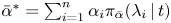 $\bar {\alpha }^{*}=\sum _{i=1}^{n} \alpha _{i} \pi _{\bar {\alpha }}(\lambda _{i}\, |\, t)$ is the weighted average of
  $\alpha _{i}$,
  $i=1,2,\ldots,n$, with weights
  $\pi _{\bar {\alpha }}(\lambda _{i}\, |\, t)$.
For the multiplicative hazard model, we have
 $$r(t \,|\, \lambda_{i})= \lambda_{i}r(t),\quad i=1,2,\ldots,n.$$
Hence, the hazard rate that corresponds to the generalized finite  $\alpha$-mixture,
  $r(t,\bar {\alpha })$, is
 \begin{align} r(t,\bar{\alpha})& =\sum_{i=1}^{n} \frac{\alpha_{i} }{\bar{\alpha}}\lambda_{i} r(t) \pi_{\bar{\alpha}}(\lambda_{i}\, |\, t) \nonumber\\ & =r(t)E_{\bar{\alpha}} (\Lambda^{*} \,|\, t). \end{align}
Thus,
 \begin{equation} r^{\prime}(t,\bar{\alpha})=r^{\prime}(t)E_{\bar{\alpha}} (\Lambda^{*} \,|\, t)+r(t) \frac{\partial}{\partial t} E_{\bar{\alpha}} (\Lambda^{*} \,|\, t). \end{equation}
From Eq. (13), the generalized finite  $\alpha$-mixture will be IFR (DFR) for
  $\alpha _{i} >0$ (
 $\alpha _{i} <0$),
  $i=1, 2, \ldots, n$, if and only if for all
  $t \in (0, \infty )$
 $$\frac{r^{\prime}(t)}{r(t)} \geq ({\leq}) -\frac{\frac{\partial}{\partial t} E_{\bar{\alpha}} (\Lambda^{*} \,|\, t)}{E_{\bar{\alpha}} (\Lambda^{*} \,|\, t)}.$$
The following theorem describes the limiting behavior of hazard rates for the multiplicative model in the generalized  $\alpha$-mixture model for two components. The result is given for positive values of
  $\alpha _{i}$,
  $i=1,2$. The case of negative values can be described in a similar manner.
Theorem 4.1 Let 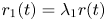 $r_{1}(t)=\lambda _{1}r(t)$,
 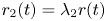 $r_{2}(t)=\lambda _{2}r(t)$ where
  $\lambda _{1} \leq \lambda _{2}$ and
  $r(t)\longrightarrow \infty$ as
  $t\longrightarrow \infty$ in the multiplicative model for the generalized finite
  $\alpha$-mixture of two SFs with
  $\alpha _{i}>0$. If
  $\alpha _{1}\leq c\alpha _{2}$, where
  $c={\lambda _{2}}/{\lambda _{1}} \geq 1$ and
  $\bar {\alpha }=p_{1} \alpha _{1}+p_{2} \alpha _{2}$, then
(a)
(14)\begin{equation} r(t,\bar{\alpha})=\frac{\alpha_{1}}{\bar{\alpha}} r_{1}(t)(1+o(1)) \quad \text{as}\ t \longrightarrow \infty. \end{equation}
(b)
(15)if and only if\begin{equation} r(t,\bar{\alpha})-\frac{\alpha_{1}}{\bar{\alpha}} r_{1}(t)\longrightarrow 0 \quad \text{as}\ t\longrightarrow \infty \end{equation}
(16)\begin{equation} r(t)\exp\left\{ -(\alpha_{2}\lambda_{2}-\alpha_{1}\lambda_{1})\int_{0}^{t} r(u)\,du\right\} \rightarrow 0 \quad \text{as}\ t\longrightarrow \infty. \end{equation}


Proof. From the assumptions of the theorem, we have  $r_{2}(t)=cr_{1}(t)$, where
  $c={\lambda _{2}}/{\lambda _{1}} \geq 1$. This implies that,
  $\bar {F}_{2}(t)=\bar {F}^{c}_{1}(t)$ and
  $f_{2}(t)=cf_{1}(t)\bar {F}^{c-1}_{1}(t)$. Thus, the ratio of the two densities and the two survival functions as
  $t\longrightarrow \infty$, is respectively,
 \begin{align*} \frac{f_{1}(t)}{f_{2}(t)}& =\frac{\bar{F}^{1-c}_{1}(t)}{c} \uparrow \infty \quad \text{if}\ c>1 \text{ and} =1\quad \text{ if } c=1\\ \frac{\bar{F}_{1}(t)}{\bar{F}_{2}(t)}& =\bar{F}^{1-c}_{1}(t) \uparrow \infty \quad \text{if}\ c>1 \ \text{and}\ =1\quad \ \text{if}\ c=1. \end{align*}
We have
 \begin{align*} \frac{r(t,\bar{\alpha})}{r_{1}(t)} & =\frac{1}{\bar{\alpha}}\times \frac{\bar{F}^{\alpha_{1}-1}_{1}(t)[ \alpha_{1}p_{1}+c \alpha_{2} p_{2}\bar{F}^{c\alpha_{2}-\alpha_{1}}_{1}(t)] \times \bar{F}_{1}(t)}{\bar{F}^{\alpha}_{1}(t)[ p_{1}+p_{2}\bar{F}^{c\alpha_{2}-\alpha_{1}}_{1}(t)] }\\ & =\frac{1}{\bar{\alpha}}\times \frac{[ \alpha_{1} p_{1}\bar{F}^{\alpha_{1}-c\alpha_{2}}_{1}(t)+c\alpha_{2}p_{2} ] \bar{F}^{c\alpha_{2}-\alpha_{1}}_{1}(t)}{[ p_{1}\bar{F}^{\alpha_{1}-c\alpha_{2}}_{1}(t)+p_{2}] \bar{F}^{c\alpha_{2}-\alpha_{1}}_{1}(t)}\\ & =\frac{1}{\bar{\alpha}}\times \left( \alpha_{1}+\frac{p_{2}(c\alpha_{2}-\alpha_{1})}{p_{1}\bar{F}^{\alpha_{1}-c\alpha_{2}}_{1}(t)+p_{2}}\right). \end{align*}
When  $t\rightarrow \infty$,
  $\bar {F}_{1}(t)\rightarrow 0$, and thus we get Eq. (14). To prove (b), note that
 \begin{equation} r(t,\bar{\alpha})-\frac{\alpha_{1}}{\bar{\alpha}} r_{1}(t) =\frac{1}{\bar{\alpha}} \times r_{1}(t)\bar{F}^{c\alpha_{2}-\alpha_{1}}_{1}(t) \frac{p_{2}(c\alpha_{2}-\alpha_{1})}{p_{1}+p_{2}\bar{F}^{c\alpha_{2}-\alpha_{1}}_{1}(t)}.\end{equation}
As
 $$r_{1}(t)\bar{F}^{c\alpha_{2}-\alpha_{1}}_{1}(t) =\lambda_{1}r(t)\exp\left\{ - (\alpha_{2}\lambda_{2}-\alpha_{1}\lambda_{1})\int_{0}^{t} r(u)\,du \right\},$$
from Eq. (16), we get
 $$r_{1}(t)\bar{F}^{c\alpha_{2}-\alpha_{1}}_{1}(t)\longrightarrow 0\quad \text{as}\ t\longrightarrow \infty,$$
Hence, from Eq. (17), we obtain the result in Eq. (15). This completes the proof.
Remark 4.1 In Theorem 4.1, since  $\lambda _{1} \leq \lambda _{2}$, we have
  $F_{1} \geq _{hr} F_{2}$, and from the results of Section 3, before Theorem 3.1, we have
  $({\alpha _{1}}/{\bar {\alpha }}) r_{1}(t) \leq r(t,\bar {\alpha })$. The results of Theorem 4.1 show the asymptotic behavior of
  $r(t,\bar {\alpha })$ in the multiplicative model. In particular, if
  $\alpha _{i}=\alpha >0$ (
 $\alpha _{i}=\alpha <0$),
  $i=1,2$, the hazard rate of the generalized finite
  $\alpha$-mixture in the multiplicative model tends to the hazard rate of the strongest (weakest) subpopulation as
  $t \rightarrow \infty$.
5. Stochastic comparisons for different baseline distributions
Our main emphasis in the rest of the paper will be on stochastic comparisons obtained by using majorization technique. However, as a prelude to that, in this section, we discuss meaningful stochastic comparisons for two generalized finite  $\alpha$-mixtures in the more conventional for existing literature way.
Theorem 5.1 Let  $F_{p}(t,\bar {\alpha })$ and
  $G_{p}(t,\bar {\alpha })$ be two n-component generalized finite
  $\alpha$-mixture models with common mixing probabilities
  $(p_{1},\ldots, p_{n})$. Assume that for
  $\alpha _{i}>0$ (
 $\alpha _{i}<0$),
  $F_{i} \leq _{st} G_{i}$ for
  $i=1,\ldots,n$. Then,
 $$F_{p}(t,\bar{\alpha}) \leq_{st} G_{p}(t,\bar{\alpha}).$$
Proof. Let  $\alpha _{i}>0 \ (\alpha _{i}<0)$. From
  $F_{i} \leq _{st} G_{i}$ for
  $i = 1,\ldots, n$, we have
  $\bar {F}_{i}(t) \leq \bar {G}_{i}(t)$ for any
  $t$,
$t$,  $i = 1,\ldots, n$. Since
  $\alpha _{i}>0\ (\alpha _{i}<0)$,
  $\bar {F}^{\alpha _{i}}_{i}(t) \leq (\geq ) \bar {G}^{\alpha _{i}}_{i}(t)$ for
  $i = 1,\ldots, n$. Thus,
 $$\sum_{i=1}^{n} p_{i}\bar{F}^{\alpha_{i}}_{i} \leq({\geq}) \sum_{i=1}^{n} p_{i}\bar{G}^{\alpha_{i}}_{i}.$$
Consequently from  $\sum _{i=1}^{n} p_{i} \alpha _{i} > 0$ (
 $\sum _{i=1}^{n} p_{i} \alpha _{i} < 0$)
 $$\left[ \sum_{i=1}^{n} p_{i}\bar{F}^{\alpha_{i}}_{i}\right]^{{1}/{\sum_{i=1}^{n} p_{i} \alpha_{i}}} \leq \left[ \sum_{i=1}^{n} p_{i}\bar{G}^{\alpha_{i}}_{i}\right]^{{1}/{\sum_{i=1}^{n} p_{i} \alpha_{i}}}.$$
This means for  $\alpha _{i}>0 \ (\alpha _{i}<0)$
 $$F_{p}(t,\bar{\alpha}) \leq_{st} G_{p}(t,\bar{\alpha}).$$
Theorem 5.2 Let  $F_{p}(t,\bar {\alpha })$ and
  $G_{p}(t,\bar {\alpha })$ be two
  $n$-component generalized finite
  $\alpha$-mixture models with common mixed proportions
  $(p_{1},\ldots, p_{n})$. Suppose that for
  $\alpha _{i} > 0 \ (\alpha _{i} < 0)$
(i)
$({\alpha _{1}}/{\bar {\alpha }}) r_{F_{1}}(t) \leq \cdots \leq ({\alpha _{n}}/{\bar {\alpha }}) r_{F_{n}}(t)$ or $({\alpha _{1}}/{\bar {\alpha }}) r_{G_{1}}(t) \leq \cdots \leq ({\alpha _{n}}/{\bar {\alpha }}) r_{G_{n}}(t)$;(ii)
${\bar {F}_{i}(t)}/{\bar {G}_{i}(t)}$ is increasing (decreasing) in $i \in \{ 1,2,\ldots,n \}$;(iii)
$F_{i} \leq _{hr} G_{i}$ for all $i \in \{ 1,2,\ldots,n \}$;(iv)
$\alpha _{1}\geq \cdots \geq \alpha _{n}$.


Then,
 $$F_{p}(t,\bar{\alpha})\leq_{hr} G_{p}(t,\bar{\alpha}).$$
Proof. Let  $\alpha _{i}>0$. From Eq. (4), the expressions for the failure rate functions that correspond to
  $F_{p}(t,\bar {\alpha })$ and
  $G_{p}(t,\bar {\alpha })$ can be written as
 $$r_{F}(t,\bar{\alpha})= \sum_{i=1}^{n} \frac{\alpha_{i}}{\bar{\alpha}} r_{F_{i}}(t) p_{\alpha_{i}}(t)$$
and
 $$r_{G}(t,\bar{\alpha})= \sum_{i=1}^{n} \frac{\alpha_{i}}{\bar{\alpha}} r_{G_{i}}(t) q_{\alpha_{i}}(t)$$
respectively, where  $q_{\alpha _{i}}(t)={p_{i} \bar {G}_{i}^{\alpha _{i}}(t)}/{\sum _{j=1}^{n} p_{j} \bar {G}_{j}^{\alpha _{j}}(t)}$ for
  $i=1,\ldots,n$. To prove
  $F_{p}(t,\bar {\alpha })\leq _{hr} G_{p}(t,\bar {\alpha })$ for
  $\alpha _{i}>0$, we need to show that
  $\psi (t)=r_{F}(t,\bar {\alpha })-r_{G}(t,\bar {\alpha })$ is non-negative for all
  $t\geq 0$. Note that,
 \begin{align*} \psi(t)& = \sum_{i=1}^{n} \frac{\alpha_{i}}{\bar{\alpha}} r_{F_{i}}(t) p_{\alpha_{i}}(t)- \sum_{i=1}^{n} \frac{\alpha_{i}}{\bar{\alpha}} r_{G_{i}}(t) q_{\alpha_{i}}(t)\\ & \geq \sum_{i=1}^{n} \frac{\alpha_{i}}{\bar{\alpha}} r_{G_{i}}(t) p_{\alpha_{i}}(t)-\sum_{i=1}^{n} \frac{\alpha_{i}}{\bar{\alpha}} r_{G_{i}}(t) q_{\alpha_{i}}(t)\equiv \xi(t), \end{align*}
where the inequality follows from condition (iii). Thus, it suffices to show that  $\xi (t)$ is non-negative for all
  $t\geq 0$. Consider two non-negative discrete random variables
  ${W}$ and
  ${V}$ on a sample space
  $\{1, \ldots, n\}$ with probability mass functions
  $q_{\alpha _{i}}(t)$ and
  $p_{\alpha _{i}}(t)$,
  $i = 1, \ldots, n$, respectively. Thus,
  $\xi (t)$ can be written as
 \begin{equation} \xi(t)=E[\phi(V)]-E[\phi(W)], \end{equation}
where  $\phi (i)=({\alpha _{i}}/{\bar {\alpha }}) r_{G_{i}}(\cdot )$,
  $i=1, \ldots,n$. To prove that Eq. (18) is non-negative, it is sufficient to show that
  $\phi (i)$ is increasing in
  $i$ and
  ${W} \leq _{st} {V}$. Based on condition (i), we have
  $({\alpha _{1}}/{\bar {\alpha }}) r_{G_{1}}(t)\leq \cdots \leq ({\alpha _{n}}/{\bar {\alpha }}) r_{G_{n}}(t)$ for all
  $t\geq 0$. Thus,
  $\phi (i)$ is increasing in
  $i$. On the other hand, one can see that
 $$\frac{p_{\alpha_{i}}(t)}{q_{\alpha_{i}}(t)} \varpropto \left(\frac{\bar{F}_{i}(t)}{\bar{G}_{i}(t)}\right)^{\alpha_{i}},\quad i \in \{1,\ldots,n\}.$$
The condition (iii), that is,  $F_{i} \leq _{hr} G_{i}$ implies
  $\bar {F}_{i}(t) \leq \bar {G}_{i}(t)$,
  $i \in \{ 1,2,\ldots,n \}$. Thus,
  $0 \leq {\bar {F}_{i}(t)}/{\bar {G}_{i}(t)} \leq 1$ for all
  $i \in \{ 1,2,\ldots,n \}$. Hence, conditions (ii) and (iv) imply that
  ${p_{\alpha _i}(t)}/{q_{\alpha _i}(t)}$ is increasing in
  $i \in \{1,\ldots,n\}$, which means that
  ${W} \leq _{lr}{V}$, which in turn implies
  ${W} \leq _{st}{V}$. Thus,
  $\xi (t)$ is non-negative and for
  $\alpha _{i}>0$,
  $F_{p}(t,\bar {\alpha })\leq _{hr}G_{p}(t,\bar {\alpha })$. If, we assume
  $({\alpha _{1}}/{\bar {\alpha }}) r_{F_{1}}(t) \leq \cdots \leq {\alpha _{n}}/{\bar {\alpha }} r_{F_{n}}(t)$, the proof is similar. The case
  $\alpha _{i}<0$ can be also established in the same way.
6. Stochastic comparisons using majorization concept
In this section, we provide the main comparison results of the paper with detailed analysis, examples and counterexamples. Specifically, we compare two generalized finite  $\alpha$-mixture in the sense of the usual stochastic order and in the sense of the hazard rate order when the vector of parameters of the first mixture majorizes the second one (see the relevant conditional characteristics discussed in Sections 3 and 4). However, first, we must recall some definitions and supplementary results to be used in what follows.
Definition 6.1 ([Reference Marshall, Olkin and Arnold21] p. 8)
Consider two vectors  $\boldsymbol {x}=(x_{1},\ldots,x_{n})$ and
  $\boldsymbol {y}=(y_{1},\ldots,y_{n})$. Let
  $x_{(1)} \leq \cdots \leq x_{(n)}$ and
  $y_{(1)} \leq \cdots \leq y_{(n)}$ be increasing arrangements of their components, respectively.
(i) If
$\sum _{j=1}^{i}x_{(j)} \leq \sum _{j=1}^{i}y_{(j)}$ for $i=1,\ldots,n-1$, and $\sum _{j=1}^{i}x_{(j)}= \sum _{j=1}^{i}y_{(j)}$, then $\boldsymbol {x}$ is said to majorize $\boldsymbol {y}$ and denoted by $\boldsymbol {x} \stackrel {m}{\succeq }\boldsymbol {y}$.(ii) If
$\sum _{j=1}^{i}x_{(j)} \leq \sum _{j=1}^{i}y_{(j)}$ for $i=1,\ldots,n$, then $\boldsymbol {x}$ is said to weakly supermajorize $\boldsymbol {y}$, and denoted by $\boldsymbol {x} \stackrel {w}{\succeq }\boldsymbol {y}$.(iii) If
$\sum _{j=i}^{n}x_{(j)} \geq \sum _{j=i}^{n}y_{(j)}$ for $i=1,\ldots,n$, then we say that $\boldsymbol {x}$ weakly submajorize $\boldsymbol {y}$, denoted by $\boldsymbol {x} {\succeq }_{w}\boldsymbol {y}$.


From the foregoing definition, clearly, the majorization order implies both weak submajorization and supermajorization orders. Order-preserving functions have been widely used in the literature to obtain some inequalities that arise from majorization. A Schur-convex function is a function that preserves the ordering of majorization [Reference Marshall, Olkin and Arnold21].
Definition 6.2 ([Reference Marshall, Olkin and Arnold21] p. 80)
A real-valued function  $\phi$ defined on a set
  $\mathbb {A} \subseteq \mathbb {R}^{n}$ is said to be Schur-convex (Schur-concave) on
  $\mathbb {A}$ if
  $\boldsymbol {x} \stackrel {m}{\succeq }\boldsymbol {y}$ implies
  $\phi (\boldsymbol {x}) \geq (\leq ) \phi (\boldsymbol {y})$ for any
  $\boldsymbol {x}, \boldsymbol {y} \in \mathbb {A}$.
Some conditions for the characterization of Schur-convex (Schur-concave) functions are provided in the next lemma.
Lemma 6.1 ([Reference Marshall, Olkin and Arnold21] p. 84)
Let  $I \subseteq \mathbb {R}$ be an open interval and let
  $\phi : I \rightarrow \mathbb {R}$ be a real-valued, continuously differentiable function. Then,
  $\phi$ is Schur-convex (Schur-concave) on
  $I^{n}$ if and only if
(i)
$\phi$ is symmetric on $I^{n}$, and(ii) for all
$i \neq j$ and all $\boldsymbol {x} \in I^{n}$,
where the partial derivative of$$(x_{i}-x_{j}) \left( \frac{\partial \phi}{\partial x_{i}}(\boldsymbol{x})-\frac{\partial \phi}{\partial x_{j}}(\boldsymbol{x})\right) \geq 0 ({\leq} 0),$$
$\phi$ with respect to its $i$th argument denoted by ${\partial \phi }/{\partial x_{i}}$.


The next lemma provides some conditions under which the weak supermajorization and the weak submajorization orders are preserved.
Lemma 6.2 ([Reference Marshall, Olkin and Arnold21] p. 87)
Consider the real-valued function  $\phi$, defined on a set
  $\mathbb {A} \subseteq \mathbb {R}^{n}$. Then,
(i)
$\boldsymbol {x}{\succeq }_{w}\boldsymbol {y}$ implies $\phi (\boldsymbol {x})\geq \phi (\boldsymbol {y})$ if and only if $\phi$ is increasing and Schur-convex on $\mathbb {A}$;(ii)
$\boldsymbol {x} \stackrel {w}{\succeq }\boldsymbol {y}$ implies $\phi (\boldsymbol {x})\geq \phi (\boldsymbol {y})$ if and only if $\phi$ is decreasing and Schur-convex on $\mathbb {A}$.


We will also need the following notation
 $$\mathcal{U}_{n}=\{ (\boldsymbol{x}, \boldsymbol{y}): x_{i}, y_{i} \geq 0 \ (x_{i}-x_{j}) (y_{i}-y_{j}) \leq 0, \ i,j=1,\ldots,n\}.$$
6.1. Usual stochastic order
Theorem 6.1 Let
 $$\bar{F}_{W_{n}(\boldsymbol{p},\boldsymbol{\lambda})}(t,\bar{\alpha}_{p})=\left[ \sum_{i=1}^{n} p_{i}{\bar{F}}^{\alpha_i}(t \,|\, \lambda_{i}) \right]^{1/\bar{\alpha}_{p}}$$
and
 $$\bar{F}_{W_{n}(\boldsymbol{p},\boldsymbol{\gamma})}(t,\bar{\alpha}_{p})=\left[ \sum_{i=1}^{n} p_{i}{\bar{F}}^{\alpha_i}(t | \gamma_{i}) \right]^{1/\bar{\alpha}_{p}},$$
be two  $n$-component generalized finite
  $\alpha$-mixtures with common mixing proportions
  $p_{1},\ldots, p_{n}$ and parameters
  $\lambda _{1},\ldots, \lambda _{n}$ and
  $\gamma _{1},\ldots, \gamma _{n}$, respectively, where
  $\bar {\alpha }_{p}=\sum _{i=1}^{n} p_{i} \alpha _{i}$. Suppose that for
  $(\boldsymbol {p}, \boldsymbol {\lambda }) \in \mathcal {U}_{n}$ and
  $(\boldsymbol {p}, \boldsymbol {\gamma }) \in \mathcal {U}_{n}$:
(i)
${\bar {F}}(t \,|\, \lambda )$ is decreasing and convex in $\lambda > 0$ for all $t \geq 0$;(ii)
$\alpha _{1}\leq \cdots, \leq \alpha _{n}$;(iii)
$\boldsymbol {\lambda } \stackrel {w}{\succeq }\boldsymbol {\gamma }$;(iv)
$\alpha _{i} p_{i} \geq \alpha _{j} p_{j}$ for all $i \leq j$, $i,j=1,2,\ldots, n$.


Then, for  $\alpha _{i} \geq 1$,
 $$\bar{F}_{W_{n}(\boldsymbol{p},\boldsymbol{\lambda})}(t,\bar{\alpha}_{p}) \geq \bar{F}_{W_{n}(\boldsymbol{p},\boldsymbol{\gamma})}(t,\bar{\alpha}_{p}).$$
Proof. Without loss of generality, suppose that  $p_{1} \geq p_{2} \geq \cdots \geq p_{n}$. From assumption
  $(\boldsymbol {p}, \boldsymbol {\lambda }) \in \mathcal {U}_{n}$ and
  $(\boldsymbol {p}, \boldsymbol {\gamma }) \in \mathcal {U}_{n}$, we have
  $0 < \lambda _{1} \leq \lambda _{2} \leq \cdots \leq \lambda _{n}$ and
  $0 < \gamma _{1} \leq \gamma _{2} \leq \cdots \leq \gamma _{n}$. Note that, by considering
  $\phi (\boldsymbol {\lambda }) = \bar {F}_{W_{n}(\boldsymbol {p},\boldsymbol {\lambda })}(t,\bar {\alpha }_{p})= [ \sum _{i=1}^{n} p_{i}{\bar {F}}^{\alpha _i}(t \,|\, \lambda _{i}) ]^{1/\bar {\alpha }_{p}}$, we have
 $$\frac{\partial \phi(\boldsymbol{\lambda}) }{\partial \lambda_{i}}= p_{i} \frac{\alpha_{i}}{\bar{\alpha}_{p}}\ \left(\frac{\partial {\bar{F}}(t \,|\, \lambda_{i})}{\partial \lambda_{i}}\right) {\bar{F}}^{\alpha_{i}-1}(t \,|\, \lambda_{i}) \left[ \sum_{i=1}^{n} p_{i}{\bar{F}}^{\alpha_{i}}(t \,|\, \lambda_{i}) \right]^{{1}/{\bar{\alpha}_{p}}-1} \leq 0,$$
as from condition (i),  $\bar {F}(t \,|\, \lambda _{i})$ is decreasing in
  $\lambda _{i}$. In addition, from Lemma 6.1 and for any pair
  $(i,j)$,
  $1 \leq i < j \leq n$,
 \begin{align*} \frac{\partial \phi(\boldsymbol{\lambda}) }{\partial \lambda_{i}}-\frac{\partial \phi(\boldsymbol{\lambda}) }{\partial \lambda_{j}}& =p_{i} \frac{\alpha_{i}}{\bar{\alpha}_{p}}\ \left(\frac{\partial {\bar{F}}(t \,|\, \lambda_{i})}{\partial \lambda_{i}}\right) {\bar{F}}^{\alpha_{i}-1}(t \,|\, \lambda_{i}) \left[ \sum_{i=1}^{n} p_{i}{\bar{F}}^{\alpha_{i}}(t \,|\, \lambda_{i}) \right]^{{1}/{\bar{\alpha}_{p}}-1}\\ & \quad - p_{j} \frac{\alpha_{j}}{\bar{\alpha}_{p}}\ \left(\frac{\partial {\bar{F}}(t \,|\, \lambda_{j})}{\partial \lambda_{j}}\right) {\bar{F}}^{\alpha_{j}-1}(t \,|\, \lambda_{j})\ \left[ \sum_{i=1}^{n} p_{i}{\bar{F}}^{\alpha_{i}}(t \,|\, \lambda_{i}) \right]^{{1}/{\bar{\alpha}_{p}}-1}. \end{align*}
This implies that
 \begin{align*} & \frac{\partial \phi(\boldsymbol{\lambda})}{\partial \lambda_{i}}-\frac{\partial \phi(\boldsymbol{\lambda}) }{\partial \lambda_{j}}\\ & \quad \stackrel{\textrm{sign}}{=} \left[ \frac{\alpha_{i}p_{i}}{\bar{\alpha}_{p}}\left(\frac{\partial {\bar{F}}(t \,|\, \lambda_{i})}{\partial \lambda_{i}}\right) {\bar{F}}^{\alpha_{i}-1}(t \,|\, \lambda_{i})-\frac{\alpha_{j}p_{j} }{\bar{\alpha}_{p}}\left(\frac{\partial {\bar{F}}(t \,|\, \lambda_{j})}{\partial \lambda_{j}}\right) {\bar{F}}^{\alpha_{j}-1}(t \,|\, \lambda_{j}) \right] \leq 0, \end{align*}
as from condition (iv),  $\alpha _{i}p_{i} \geq \alpha _{j} p_{j}$ and from condition (i),
  $\bar {F}(t \,|\, \lambda _{i})$ is decreasing and convex, thus
  $-{(\partial {\bar {F}}(t \,|\, \lambda _{i}))}/{\partial \lambda _{i}} \geq -{(\partial {\bar {F}}(t \,|\, \lambda _{j}))}/{\partial \lambda _{j}} \geq 0$ and from condition (ii),
  ${\bar {F}}^{\alpha _{i}-1}(t \,|\, \lambda _{i}) \geq {\bar {F}}^{\alpha _{j}-1}(t \,|\, \lambda _{j})$. Thus,
 $$(\lambda_{i}-\lambda_{j}) \left(\frac{\partial \phi(\boldsymbol{\lambda})}{\partial \lambda_{i}}-\frac{\partial \phi(\boldsymbol{\lambda}) }{\partial \lambda_{j}} \right) \geq 0.$$
Consequently,  $\bar {F}_{W_{n}(\boldsymbol {p},\boldsymbol {\lambda })}(t,\bar {\alpha }_{p})$ is decreasing and Schur-convex for
  $\alpha _{i} \geq 1$. Now, condition (iii),
  $\boldsymbol {\lambda } \stackrel {w} {\succeq } \boldsymbol {\gamma }$, together with condition of Lemma 6.2 imply
  $\phi (\boldsymbol {\lambda }) \geq \phi (\boldsymbol {\gamma })$. This means
  $\bar {F}_{W_{n}(\boldsymbol {p},\boldsymbol {\lambda })}(t,\bar {\alpha }_{p})\geq \bar {F}_{W_{n}(\boldsymbol {p},\boldsymbol {\gamma })}(t,\bar {\alpha }_{p})$ completing the proof of the theorem.
Remark 6.1 Theorem 6.1 extends the result of Theorem 3.2 in Nadeb and Torabi [Reference Nadeb and Torabi23] that compares two finite ordinary mixtures with respect to parameter  $\lambda$.
To illustrate Theorem 6.1, we present a numerical example.
Example 6.1 Let  $\bar {F}(t \,|\, \lambda )=e^{-\lambda t}$, for
  $t \in [0,+\infty )$. Clearly,
  $\bar {F}(t \,|\, \lambda )$ is decreasing and convex in
  $\lambda$. Set
  $(p_{1}, p_{2}, p_{3})=(0.55, 0.35, 0.1)$,
  $(\lambda _{1}, \lambda _{2}, \lambda _{3})=(0.4, 0.7, 0.8)$,
  $(\gamma _{1}, \gamma _{2}, \gamma _{3})=(0.5, 0.8, 0.9)$ and
  $(\alpha _{1}, \alpha _{2}, \alpha _{3})=(2.5, 3,4)$. As we see,
  $\boldsymbol {\lambda }\stackrel {w} {\succeq }\boldsymbol {\gamma }$,
  $(\boldsymbol {p},\boldsymbol {\lambda }) \in \mathcal {U}_{3}$ and
  $(\boldsymbol {p},\boldsymbol {\gamma }) \in \mathcal {U}_{3}$ and
  $(\alpha _{1}p_{1}, \alpha _{2}p_{2}, \alpha _{3}p_{3})=(1.375, 1.05,0.4)$. Thus, all conditions of Theorem 6.1 are satisfied.
However, if conditions  $(\boldsymbol {p},\boldsymbol {\lambda }) \in \mathcal {U}_{n}$ and
  $(\boldsymbol {p},\boldsymbol {\gamma }) \in \mathcal {U}_{n}$ in Theorem 6.1 are removed, the result may be not true any more. The following counterexample illustrates this.
Counterexample 6.1 In Example 6.1, set  $(\lambda _{1}, \lambda _{2}, \lambda _{3})=(18, 5, 1)$ and
  $(\gamma _{1}, \gamma _{2}, \gamma _{3})=(17, 5, 2)$. Thus,
  $(\boldsymbol {p},\boldsymbol {\lambda }) \notin \mathcal {U}_{3}$ and
  $(\boldsymbol {p},\boldsymbol {\gamma }) \notin \mathcal {U}_{3}$. Figure 2 plots
  $\bar {F}_{W_{3}(\boldsymbol {p},\boldsymbol {\lambda })}(t,\bar {\alpha }_{p})$,
  $\bar {F}_{W_{3}(\boldsymbol {p},\boldsymbol {\gamma })}(t,\bar {\alpha }_{p})$ and
  $g_{1}(t)=\bar {F}_{W_{3}(\boldsymbol {p},\boldsymbol {\lambda })}(t,\bar {\alpha }_{p})-\bar {F}_{W_{3}(\boldsymbol {p},\boldsymbol {\gamma })}(t,\bar {\alpha }_{p})$, which indicates that the usual stochastic ordering does not hold between
  $\bar {F}_{W_{3}(\boldsymbol {p},\boldsymbol {\lambda })}(t,\bar {\alpha }_{p})$ and
  $\bar {F}_{W_{3}(\boldsymbol {p},\boldsymbol {\gamma })}(t,\bar {\alpha }_{p})$.

Figure 2. (a) The plots of  $\bar {F}_{W_{3}(\boldsymbol {p},\boldsymbol {\lambda })}(t,\bar {\alpha }_{p})$ (solid) and
  $\bar {F}_{W_{3}(\boldsymbol {p},\boldsymbol {\gamma })}(t,\bar {\alpha }_{p})$ (dash dot). (b)
  $g_{1}(t)=\bar {F}_{W_{3}(\boldsymbol {p},\boldsymbol {\lambda })}(t,\bar {\alpha }_{p})-\bar {F}_{W_{3}(\boldsymbol {p},\boldsymbol {\gamma })}(t,\bar {\alpha }_{p})$.
Theorem 6.2 Let  $\bar {F}_{W_{n}(\boldsymbol {p},\boldsymbol {\lambda })}(t,\bar {\alpha }_{p})$ and
  $\bar {F}_{W_{n}(\boldsymbol {p},\boldsymbol {\gamma })}(t,\bar {\alpha }_{p})$ be two
  $n$-component generalized finite
  $\alpha$-mixtures with common mixing proportions
  $p_{1},\ldots, p_{n}$ and parameters
  $\lambda _{1},\ldots, \lambda _{n}$ and
  $\gamma _{1},\ldots, \gamma _{n}$, respectively, where
  $\bar {\alpha }_{p}=\sum _{i=1}^{n} p_{i} \alpha _{i}$. Suppose that for
  $(\boldsymbol {p}, \boldsymbol {\lambda }) \in \mathcal {U}_{n}$ and
  $(\boldsymbol {p}, \boldsymbol {\gamma }) \in \mathcal {U}_{n}$:
(i)
${\bar {F}}(t \,|\, \lambda )$ is increasing and concave in $\lambda > 0$ for all $t \geq 0$;(ii)
$\alpha _{1}\leq \cdots, \leq \alpha _{n}$;(iii)
$\boldsymbol {\lambda } \stackrel {w}{\succeq }\boldsymbol {\gamma }$.


Then, for  $\alpha _{i} \leq 0$ (
 $0 < \alpha _{i} < 1$ such that
  $\alpha _{i} p_{i} \geq \alpha _{j} p_{j}$ for all
  $i \leq j$,
  $i,j=1,2,\ldots, n$):
 $$\bar{F}_{W_{n}(\boldsymbol{p},\boldsymbol{\lambda})}(t,\bar{\alpha}_{p}) \leq \bar{F}_{W_{n}(\boldsymbol{p},\boldsymbol{\gamma})}(t,\bar{\alpha}_{p}).$$
The proof of this theorem is similar (with relevant alterations) to that of the previous one and, therefore, is omitted. To illustrate the result, the following numerical example is provided.
Example 6.2 Let  $\bar {F}(t \,|\, \lambda )=({\lambda }/{(\lambda +t^{2})})^{a}$, for
  $t \in [0,+\infty )$, which is the survival function of the Compound Rayleigh distribution. Clearly,
  $\bar {F}(t \,|\, \lambda )$ is increasing and concave in
  $\lambda$ for
  $0 < a < 1$. For
  $\alpha _{i} \leq 0$ (
 $0 < \alpha _{i} < 1$), set
  $a=0.9$,
  $(p_{1}, p_{2}, p_{3})=(0.6, 0.3, 0.1)$,
  $(\lambda _{1}, \lambda _{2}, \lambda _{3})=(10, 12, 14)$,
  $(\gamma _{1}, \gamma _{2}, \gamma _{3})=(11, 12, 15)$ and
  $(\alpha _{1}, \alpha _{2}, \alpha _{3})=(-4, -3,-2.5)$ (
 $(\alpha _{1}, \alpha _{2}, \alpha _{3})=(0.4, 0.5,0.6$)). As we see,
  $\boldsymbol {\lambda }\stackrel {w} {\succeq }\boldsymbol {\gamma }$,
  $(\boldsymbol {p},\boldsymbol {\lambda }) \in \mathcal {U}_{3}$ and
  $(\boldsymbol {p},\boldsymbol {\gamma }) \in \mathcal {U}_{3}$ and for
  $0 < \alpha _{i} < 1$,
  $(\alpha _{1}p_{1}, \alpha _{2}p_{2}, \alpha _{3}p_{3})=(0.24, 0.15,0.06)$. Thus, all conditions of Theorem 6.2 are satisfied.
In the following counterexample, we show that conditions  $(\boldsymbol {p},\boldsymbol {\lambda }) \in \mathcal {U}_{n}$ and
  $(\boldsymbol {p},\boldsymbol {\gamma }) \in \mathcal {U}_{n}$ in Theorem 6.9 can not be dropped.
Counterexample 6.2 In Example 6.2, set  $(\lambda _{1}, \lambda _{2}, \lambda _{3})=(20, 10.5, 10)$ and
  $(\gamma _{1}, \gamma _{2}, \gamma _{3})=(19.5, 11, 10)$. Thus,
  $(\boldsymbol {p},\boldsymbol {\lambda }) \notin \mathcal {U}_{3}$ and
  $(\boldsymbol {p},\boldsymbol {\gamma }) \notin \mathcal {U}_{3}$. Figure 3 plots
  $g_{2}(t)=\bar {F}_{W_{3}(\boldsymbol {p},\boldsymbol {\gamma })}(t,\bar {\alpha }_{p})-\bar {F}_{W_{3}(\boldsymbol {p},\boldsymbol {\lambda })}(t,\bar {\alpha }_{p})$ for
  $\alpha _{i} \leq 0$ and
  $0 < \alpha _{i} < 1$, which indicates that the usual stochastic ordering does not hold between
  $\bar {F}_{W_{3}(\boldsymbol {p},\boldsymbol {\lambda })}(t,\bar {\alpha }_{p})$ and
  $\bar {F}_{W_{3}(\boldsymbol {p},\boldsymbol {\gamma })}(t,\bar {\alpha }_{p})$.

Figure 3. (a)  $g_{2}(t)=\bar {F}_{W_{3}(\boldsymbol {p},\boldsymbol {\gamma })}(t,\bar {\alpha }_{p})-\bar {F}_{W_{3}(\boldsymbol {p},\boldsymbol {\lambda })}(t,\bar {\alpha }_{p})$ for
  $\alpha _{i} \leq 0$. (b)
  $g_{2}(t)=\bar {F}_{W_{3}(\boldsymbol {p},\boldsymbol {\gamma })}(t,\bar {\alpha }_{p})-\bar {F}_{W_{3}(\boldsymbol {p},\boldsymbol {\lambda })}(t,\bar {\alpha }_{p})$ for
  $0 < \alpha _{i} < 1$.
Corollary 6.1 Let  $\bar {F}(t \,|\, \lambda )$ belongs to the proportional hazard family,
  $\bar {F}(t \,|\, \lambda )={\bar {F}}^{\lambda }(t)$, for all
  $t$, where
  $\bar {F}(t)$ is the baseline survival function. Then, for
  $\alpha _{i} \geq 1$,
  $i=1,2, \ldots, n$ such that
  $\alpha _{1} \leq \alpha _{2} \leq \cdots \leq \alpha _{n}$ and
  $\alpha _{i} p_{i} \geq \alpha _{j} p_{j}$ for all
  $i \leq j, i,j=1,2, \ldots, n$,
  $\boldsymbol {\lambda }\stackrel {w}{\succeq }\boldsymbol {\gamma }$,
  $(\boldsymbol {p}, \boldsymbol {\lambda }) \in \mathcal {U}_{n}$ and
  $(\boldsymbol {p}, \boldsymbol {\gamma }) \in \mathcal {U}_{n}$, we have
 $$\bar{F}_{W_{n}(\boldsymbol{p},\boldsymbol{\lambda})}(t,\bar{\alpha}_{p}) \geq \bar{F}_{W_{n}(\boldsymbol{p},\boldsymbol{\gamma})}(t,\bar{\alpha}_{p}).$$
Corollary 6.2 Let  $\bar {F}(t \,|\, \lambda )$ belong to the accelerated lifetime (scale model) family,
  $\bar {F}(t \,|\, \lambda )=\bar {F}(\lambda t)$, for all
  $t$, where
  $\bar {F}(t)$ is the baseline survival function. Also, let
  $f(t)$ denoting the baseline density function, is decreasing in
  $t$. Then, for
  $\alpha _{i} \geq 1$,
  $i=1,2, \ldots, n$ such that
  $\alpha _{1} \leq \alpha _{2} \leq \cdots \leq \alpha _{n}$ and
  $\alpha _{i} p_{i} \geq \alpha _{j} p_{j}$ for all
  $i \leq j, i,j=1,2, \ldots, n$,
  $\boldsymbol {\lambda }\stackrel {w}{\succeq }\boldsymbol {\gamma }$,
  $(\boldsymbol {p}, \boldsymbol {\lambda }) \in \mathcal {U}_{n}$ and
  $(\boldsymbol {p}, \boldsymbol {\gamma }) \in \mathcal {U}_{n}$, we have
 $$\bar{F}_{W_{n}(\boldsymbol{p},\boldsymbol{\lambda})}(t,\bar{\alpha}_{p}) \geq \bar{F}_{W_{n}(\boldsymbol{p},\boldsymbol{\gamma})}(t,\bar{\alpha}_{p}).$$
Corollary 6.3 Let  $\bar {F}(t \,|\, \lambda )$ belong to the proportional reversed hazard family,
  $\bar {F}(t \,|\, \lambda )=1-{F}^{\lambda }(t)$, for all
  $t$, where
  $F(t)$ is the baseline distribution function. Then, for
  $\alpha _{i} \leq 0$ (
 $0 < \alpha _{i} < 1$ such that
  $\alpha _{i} p_{i} \geq \alpha _{j} p_{j}$ for all
  $i \leq j, i,j=1,2, \ldots, n$),
  $i=1,2, \ldots, n$ such that
  $\alpha _{1} \leq \alpha _{2} \leq \cdots \leq \alpha _{n}$,
  $\boldsymbol {\lambda }\stackrel {w}{\succeq }\boldsymbol {\gamma }$,
  $(\boldsymbol {p}, \boldsymbol {\lambda }) \in \mathcal {U}_{n}$ and
  $(\boldsymbol {p}, \boldsymbol {\gamma }) \in \mathcal {U}_{n}$, we have
 $$\bar{F}_{W_{n}(\boldsymbol{p},\boldsymbol{\lambda})}(t,\bar{\alpha}_{p}) \leq \bar{F}_{W_{n}(\boldsymbol{p},\boldsymbol{\gamma})}(t,\bar{\alpha}_{p}).$$
From Theorems 6.1 and 6.2, we can obtain a lower or upper bound for the generalized finite  $\alpha$-mixture as discussed in the following remark.
Remark 6.2 Set  $(\gamma _{1}, \ldots, \gamma _{n})=(\bar {\lambda }, \ldots, \bar {\lambda })$, where
  $\bar {\lambda }=({1}/{n}) \sum _{i=1}^{n} \lambda _{i}$. It is easy to see that
  $\boldsymbol {\lambda }\stackrel {w}{\succeq }\boldsymbol {\gamma }$. Then, for
  $(\boldsymbol {p}, \boldsymbol {\lambda }) \in \mathcal {U}_{n}$:
(i) If
$\bar {F}(t \,|\, \lambda )$ is decreasing and convex in $\lambda > 0$ for all $t$ and for $\alpha _{i} \geq 1$, $i=1,2, \ldots, n$ such that $\alpha _{1} \leq \alpha _{2} \leq \cdots \leq \alpha _{n}$ and $\alpha _{i} p_{i} \geq \alpha _{j} p_{j}$ for all $i \leq j, i,j=1,2, \ldots, n$, we have the following lower bound for the generalized finite $\alpha$-mixture:
$$\bar{F}_{W_{n}(\boldsymbol{p},\boldsymbol{\lambda})}(t,\bar{\alpha}_{p}) \geq {\bar{F}}^{{\alpha_{n}}/{\bar{\alpha}_{p}}} (t \,| \,\bar{\lambda}).$$
(ii) If
$\bar {F}(t \,|\, \lambda )$ is increasing and concave in $\lambda > 0$ for all $t$ and for $\alpha _{i} \leq 0$ ($0 < \alpha _{i} < 1$ such that $\alpha _{i} p_{i} \geq \alpha _{j} p_{j}$ for all $i \leq j, i,j=1,2, \ldots, n$), $i=1,2, \ldots, n$ such that $\alpha _{1} \leq \alpha _{2} \leq \cdots \leq \alpha _{n}$, we have the following upper bound for the generalized finite $\alpha$-mixture:
$$\bar{F}_{W_{n}(\boldsymbol{p},\boldsymbol{\lambda})}(t,\bar{\alpha}_{p}) \leq {\bar{F}}^{\frac{\alpha_{n}}{\bar{\alpha}_{p}}} (t \,| \,\bar{\lambda}).$$


The next numerical examples illustrate Remark 6.2 for two cases  $\alpha _{i} \geq 1$ and
  $\alpha _{i} \leq 0$.
Example 6.3
(i) Consider Example 6.1. Let
$\bar {F}(t \,|\, \lambda )=e^{-\lambda t}$, for $t \in [0,+\infty )$. Clearly, $\bar {F}(t \,|\, \lambda )$ is decreasing and convex in $\lambda$. Set $(p_{1}, p_{2}, p_{3})=(0.55, 0.35, 0.1)$, $(\lambda _{1}, \lambda _{2}, \lambda _{3})=(0.4, 0.7, 0.8)$, $(\gamma _{1}, \gamma _{2}, \gamma _{3})=(\bar {\lambda },\bar {\lambda },\bar {\lambda })=(0.63, 0.63, 0.63)$ and $(\alpha _{1}, \alpha _{2}, \alpha _{3})=(2.5, 3,4)$. As we see, $\boldsymbol {\lambda }\stackrel {w} {\succeq }\boldsymbol {\gamma }$, $(\boldsymbol {p},\boldsymbol {\lambda }) \in \mathcal {U}_{3}$ and $(\boldsymbol {p},\boldsymbol {\bar {\lambda }}) \in \mathcal {U}_{3}$ and $(\alpha _{1}p_{1}, \alpha _{2}p_{2}, \alpha _{3}p_{3})=(1.375, 1.05,0.4)$. Thus, all conditions of Remark 6.2(i) are satisfied.(ii) Consider Example 6.2. Let
$\bar {F}(t | \lambda )=({\lambda }/{(\lambda +t^{2}}))^{a}$, for $t \in [0,+\infty )$, which is the survival function of the Compound Rayleigh distribution. Clearly, $\bar {F}(t\, |\, \lambda )$ is increasing and concave in $\lambda$ for $0 < a < 1$. For $\alpha _{i} \leq 0$, set $a=0.9$, $(p_{1}, p_{2}, p_{3})=(0.6, 0.3, 0.1)$, $(\lambda _{1}, \lambda _{2}, \lambda _{3})=(10, 12, 14)$, $(\gamma _{1}, \gamma _{2}, \gamma _{3})=(\bar {\lambda },\bar {\lambda },\bar {\lambda })=(12, 12, 12)$ and $(\alpha _{1}, \alpha _{2}, \alpha _{3})=(-4, -3,-2.5)$. As we see, $\boldsymbol {\lambda }\stackrel {w} {\succeq }\boldsymbol {\gamma }$, $(\boldsymbol {p},\boldsymbol {\lambda }) \in \mathcal {U}_{3}$ and $(\boldsymbol {p},\boldsymbol {\bar {\lambda }}) \in \mathcal {U}_{3}$. Thus, all conditions of Remark 6.2(ii) are satisfied.


6.2. Hazard rate order
In this subsection, we consider the  $2$-component generalized finite
  $\alpha$-mixture and provide some comparisons in the sense of the hazard rate order.
Theorem 6.3 Let
 $$\bar{F}_{W_{2}(\boldsymbol{p},\boldsymbol{\lambda})}(t,\bar{\alpha}_{p})=\left[ \sum_{i=1}^{2} p_{i}{\bar{F}}^{\alpha_i}(t \,|\, \lambda_{i}) \right]^{1/\bar{\alpha}_{p}}$$
and
 $$\bar{F}_{W_{2}(\boldsymbol{p},\boldsymbol{\gamma})}(t,\bar{\alpha}_{p})=\left[ \sum_{i=1}^{2} p_{i}{\bar{F}}^{\alpha_i}(t \,|\, \gamma_{i}) \right]^{1/\bar{\alpha}_{p}},$$
be two  $2$-component generalized finite
  $\alpha$-mixtures with common mixing proportions
  $p_{1}, p_{2}$ and parameters
  $\lambda _{1}, \lambda _{2}$ and
  $\gamma _{1}, \gamma _{2}$, respectively, where
  $\bar {\alpha }_{p}=\sum _{i=1}^{2} p_{i} \alpha _{i}$. Suppose that for
  $(\boldsymbol {p}, \boldsymbol {\lambda }) \in \mathcal {U}_{2}$ and
  $(\boldsymbol {p}, \boldsymbol {\gamma }) \in \mathcal {U}_{2}$:
(i)
$r(t \,|\, \lambda )$ is increasing (decreasing) and concave (convex) in $\lambda > 0$ for all $t$;(ii)
$\bar {F}(t \,|\, \lambda )$ is decreasing (increasing) in $\lambda > 0$ for all $t$;(iii)
$\alpha _{1}\leq \alpha _{2}$;(iv)
$\boldsymbol {\lambda } \stackrel {m}{\succeq }\boldsymbol {\gamma }$.


Then, for  $\alpha _{i} \geq 0$ such that
  $\alpha _{1} p_{1} \geq \alpha _{2} p_{2}$ (
 $\alpha _{i} < 0$) :
 $$r_{W_{2}(\boldsymbol{p},\boldsymbol{\lambda})}(t,\bar{\alpha}_{p}) \leq ({\geq}) r_{W_{2}(\boldsymbol{p},\boldsymbol{\gamma})}(t,\bar{\alpha}_{p}),$$
where  $r_{W_{2}(\boldsymbol {p},\boldsymbol {\lambda })}(t,\bar {\alpha }_{p})$ and
  $r_{W_{2}(\boldsymbol {p},\boldsymbol {\gamma })}(t,\bar {\alpha }_{p})$ are the hazard rate functions that correspond to
  $\bar {F}_{W_{2}(\boldsymbol {p},\boldsymbol {\lambda })}(t,\bar {\alpha }_{p})$ and
  $\bar {F}_{W_{2}(\boldsymbol {p},\boldsymbol {\gamma })}(t,\bar {\alpha }_{p})$, respectively.
Proof. Without loss of generality, suppose that  $p_{1} \geq p_{2}$. From assumption
  $(\boldsymbol {p}, \boldsymbol {\lambda }) \in \mathcal {U}_{2}$ and
  $(\boldsymbol {p}, \boldsymbol {\gamma }) \in \mathcal {U}_{2}$, we have
  $0 < \lambda _{1} \leq \lambda _{2}$ and
  $0 < \gamma _{1} \leq \gamma _{2}$. The hazard rate function of
  $\bar {F}_{W_{2}(\boldsymbol {p},\boldsymbol {\lambda }})(t,\bar {\alpha }_{p})$ is
 \begin{align*} r_{W_{2}(\boldsymbol{p},\boldsymbol{\lambda})}(t,\bar{\alpha}_{p})& =\frac{1}{\bar{\alpha}_{p}} \left[ \frac{\sum_{i=1}^{2} p_{i} \alpha_{i} r(t \,|\, \lambda_{i}) {\bar{F}}^{\alpha_{i}}(t \,|\, \lambda_{i}) }{\sum_{i=1}^{2} p_{i} {\bar{F}}^{\alpha_{i}}(t \,|\, \lambda_{i})} \right]\\ & =\frac{1}{\bar{\alpha}_{p}} \left[ \frac{ p_{1} \alpha_{1} r(t \,|\, \lambda_{1}) {\bar{F}}^{\alpha_{1}}(t \,|\, \lambda_{1})+p_{2} \alpha_{2} r(t \,|\, \lambda_{2}) {\bar{F}}^{\alpha_{2}}(t \,|\, \lambda_{2}) }{ p_{1} {\bar{F}}^{\alpha_1}(t \,|\, \lambda_{1})+p_{2} {\bar{F}}^{\alpha_{2}}(t \,|\, \lambda_{2})} \right]\\ & =\frac{1}{\bar{\alpha}_{p}} \left[ \frac{\Psi_{1}(t; \boldsymbol{p}, \boldsymbol{\lambda})}{\Psi_{2}(t; \boldsymbol{p}, \boldsymbol{\lambda})} \right]. \end{align*}
Thus,
 \begin{align*} \frac{\partial r_{W_{2}(\boldsymbol{p},\boldsymbol{\lambda})}(t,\bar{\alpha}_{p})}{\partial \lambda_{1}}& =\frac{1}{\bar{\alpha}_{p}} \left[ \dfrac{\frac{\partial \Psi_{1}(t; \boldsymbol{p}, \boldsymbol{\lambda})}{\partial \lambda_{1}} \Psi_{2}(t; \boldsymbol{p}, \boldsymbol{\lambda})-\frac{\partial \Psi_{2}(t; \boldsymbol{p}, \boldsymbol{\lambda})}{\partial \lambda_{1}} \Psi_{1}(t; \boldsymbol{p}, \boldsymbol{\lambda})}{\Psi^{2}_{2}(t; \boldsymbol{p}, \boldsymbol{\lambda})}\right]\\ & \stackrel{\textrm{sign}}{=} \frac{1}{\bar{\alpha}_{p}} \left[ p_{1} \alpha_{1} \left( \frac{\partial r(t \,|\, \lambda_{1}) }{\partial \lambda_{1}} {\bar{F}}^{\alpha_{1}}(t \,|\, \lambda_{1})+ \alpha_{1} \frac{\partial {\bar{F}}(t \,|\, \lambda_{1}) }{\partial \lambda_{1}} {\bar{F}}^{\alpha_{1}-1}(t \,|\, \lambda_{1}) r(t \,|\, \lambda_{1}) \right) \Psi_{2}(t; \boldsymbol{p}, \boldsymbol{\lambda})\right.\\ & \quad \left.- \left( p_{1} \alpha_{1} \frac{\partial {\bar{F}}(t \,|\, \lambda_{1}) }{\partial \lambda_{1}} {\bar{F}}^{\alpha_{1}-1}(t \,|\, \lambda_{1}) \right) \Psi_{1}(t; \boldsymbol{p}, \boldsymbol{\lambda}) \right]\\ & = \frac{ p_{1} \alpha_{1} }{\bar{\alpha}_{p}} \left[ \frac{\partial r(t \,|\, \lambda_{1}) }{\partial \lambda_{1}} {\bar{F}}^{\alpha_{1}}(t \,|\, \lambda_{1}) \Psi_{2}(t; \boldsymbol{p}, \boldsymbol{\lambda})+ \alpha_{1} \frac{\partial {\bar{F}}(t \,|\, \lambda_{1}) }{\partial \lambda_{1}} {\bar{F}}^{\alpha_{1}-1}(t \,|\, \lambda_{1}) r(t \,|\, \lambda_{1}) \Psi_{2}(t; \boldsymbol{p}, \boldsymbol{\lambda})\right.\\ & \quad \left.- \frac{\partial {\bar{F}}(t \,|\, \lambda_{1}) }{\partial \lambda_{1}} {\bar{F}}^{\alpha_{1}-1}(t \,|\, \lambda_{1}) \Psi_{1}(t; \boldsymbol{p}, \boldsymbol{\lambda}) \right]\\ & =\frac{ p_{1} \alpha_{1} }{\bar{\alpha}_{p}} \left[ \frac{\partial r(t \,|\, \lambda_{1}) }{\partial \lambda_{1}} {\bar{F}}^{\alpha_{1}}(t \,|\, \lambda_{1}) \Psi_{2}(t; \boldsymbol{p}, \boldsymbol{\lambda})\right.\\ & \quad \left.+ \frac{\partial {\bar{F}}(t \,|\, \lambda_{1}) }{\partial \lambda_{1}} {\bar{F}}^{\alpha_{1}-1}(t \,|\, \lambda_{1}) \left( \alpha_{1} r(t \,|\, \lambda_{1}) \Psi_{2}(t; \boldsymbol{p}, \boldsymbol{\lambda}) - \Psi_{1}(t; \boldsymbol{p}, \boldsymbol{\lambda}) \right) \right]\\ & =\frac{ p_{1} \alpha_{1} }{\bar{\alpha}_{p}} \left[ \frac{\partial r(t \,|\, \lambda_{1}) }{\partial \lambda_{1}} {\bar{F}}^{\alpha_{1}}(t \,|\, \lambda_{1}) \Psi_{2}(t; \boldsymbol{p}, \boldsymbol{\lambda})\right.\\ & \quad \left.+ \frac{\partial {\bar{F}}(t \,|\, \lambda_{1}) }{\partial \lambda_{1}} {\bar{F}}^{\alpha_{1}-1}(t \,|\, \lambda_{1}) ( p_{2} {\bar{F}}^{\alpha_{2}}(t \,|\, \lambda_{2}) ( \alpha_{1} r(t \,|\, \lambda_{1})- \alpha_{2} r(t \,|\, \lambda_{2}))) \right]. \end{align*}
Now, we have
 \begin{align*} & \frac{\partial r_{W_{2}(\boldsymbol{p},\boldsymbol{\lambda})}(t,\bar{\alpha}_{p})}{\partial \lambda_{1}}-\frac{\partial r_{W_{2}(\boldsymbol{p},\boldsymbol{\lambda})}(t,\bar{\alpha}_{p})}{\partial \lambda_{2}}\\ & \quad \stackrel{\textrm{sign}}{=} \frac{1}{\bar{\alpha}_{p}} \left[ \left( p_{1} \alpha_{1} \frac{\partial r(t \,|\, \lambda_{1}) }{\partial \lambda_{1}} {\bar{F}}^{\alpha_{1}}(t \,|\, \lambda_{1})-p_{2} \alpha_{2} \frac{\partial r(t \,|\, \lambda_{2}) }{\partial \lambda_{2}} {\bar{F}}^{\alpha_{2}}(t \,|\, \lambda_{2}) \right) \Psi_{2}(t; \boldsymbol{p}, \boldsymbol{\lambda})\right]\\ & \qquad + \frac{1}{\bar{\alpha}_{p}} \left[ p_{1} \alpha_{1} \frac{\partial {\bar{F}}(t \,|\, \lambda_{1}) }{\partial \lambda_{1}} {\bar{F}}^{\alpha_{1}-1}(t \,|\, \lambda_{1}) ( p_{2} {\bar{F}}^{\alpha_{2}}(t \,|\, \lambda_{2}) ( \alpha_{1} r(t \,|\, \lambda_{1})- \alpha_{2} r(t \,|\, \lambda_{2})) )\right.\\ & \qquad \left.-p_{2} \alpha_{2} \frac{\partial {\bar{F}}(t \,|\, \lambda_{2}) }{\partial \lambda_{2}} {\bar{F}}^{\alpha_{2}-1}(t \,|\, \lambda_{2}) ( p_{1} {\bar{F}}^{\alpha_{1}}(t \,|\, \lambda_{1}) ( \alpha_{2} r(t \,|\, \lambda_{2})- \alpha_{1} r(t \,|\, \lambda_{1})) ) \right]\\ & \quad =\frac{1}{\bar{\alpha}_{p}} [ A+B-C ], \end{align*}
where,
 \begin{align*} A& =\left( p_{1} \alpha_{1} \frac{\partial r(t \,|\, \lambda_{1}) }{\partial \lambda_{1}} {\bar{F}}^{\alpha_{1}}(t \,|\, \lambda_{1})-p_{2} \alpha_{2} \frac{\partial r(t \,|\, \lambda_{2}) }{\partial \lambda_{2}} {\bar{F}}^{\alpha_{2}}(t \,|\, \lambda_{2}) \right) \Psi_{2}(t; \boldsymbol{p}, \boldsymbol{\lambda}),\\ B& =p_{1} \alpha_{1} \frac{\partial {\bar{F}}(t \,|\, \lambda_{1}) }{\partial \lambda_{1}} {\bar{F}}^{\alpha_{1}-1}(t \,|\, \lambda_{1}) ( p_{2} {\bar{F}}^{\alpha_{2}}(t \,|\, \lambda_{2}) ( \alpha_{1} r(t \,|\, \lambda_{1})- \alpha_{2} r(t \,|\, \lambda_{2})) ) \end{align*}
and
 $$C=p_{2} \alpha_{2} \frac{\partial {\bar{F}}(t \,|\, \lambda_{2}) }{\partial \lambda_{2}} {\bar{F}}^{\alpha_{2}-1}(t \,|\, \lambda_{2}) ( p_{1} {\bar{F}}^{\alpha_{1}}(t \,|\, \lambda_{1}) ( \alpha_{2} r(t \,|\, \lambda_{2})- \alpha_{1} r(t \,|\, \lambda_{1})) ).$$
From condition (ii),  ${\bar {F}}(t \,|\, \lambda _{1}) \geq (\leq ) {\bar {F}}(t \,|\, \lambda _{2})$. Since, from condition (iii),
  $\alpha _{1} \leq \alpha _{2}$,
  ${\bar {F}}^{\alpha _{1}}(t \,|\, \lambda _{1}) \geq {\bar {F}}^{\alpha _{2}}(t \,|\, \lambda _{2})$. From condition (i),
  ${(\partial r(t \,|\, \lambda _{1}))}/{\partial \lambda _{1}} \geq (\leq ) {(\partial r(t \,|\, \lambda _{2}))}/{\partial \lambda _{2}} \geq (\leq ) 0$. Consequently,
  $A \geq 0$ follows from condition
  $\alpha _{1}p_{1} \geq \alpha _{2}p_{2}$. Also, we claim that
  $B \geq 0$, because from condition (i),
  $r(t \,|\, \lambda _{1}) \leq (\geq ) r(t \,|\, \lambda _{2})$, and condition (iii),
  $\alpha _{1} \leq \alpha _{2}$,
  $( \alpha _{1} r(t \,|\, \lambda _{1}) - \alpha _{2} r(t \,|\, \lambda _{2})) \leq 0$. On the other hand, from condition (ii),
  ${\partial {\bar {F}}(t \,|\, \lambda _{1}) }/{\partial \lambda _{1}} \leq (\geq ) 0$. Consequently,
  $B \geq 0$. Similarly,
  $C \leq 0$ and hence
  $-C \geq 0$. Therefore,
 $$(\lambda_{1}-\lambda_{2})\left( \frac{\partial r_{W_{2}(\boldsymbol{p},\boldsymbol{\lambda})}(t,\bar{\alpha_{p}})}{\partial \lambda_{1}}-\frac{\partial r_{W_{2}(\boldsymbol{p},\boldsymbol{\lambda})}(t,\bar{\alpha_{p}})}{\partial \lambda_{2}} \right) \leq ({\geq}) 0.$$
Consequently, according to Lemma 6.1,  $r_{W_{2}(\boldsymbol {p},\boldsymbol {\lambda })}(t,\bar {\alpha _{p}})$ is Schur-concave (Schur-convex). Using condition (iv),
  $\boldsymbol {\lambda } \stackrel {m}{\succeq }\boldsymbol {\gamma }$, we have
  $r_{W_{2}(\boldsymbol {p},\boldsymbol {\lambda })}(t,\bar {\alpha }_{p}) \leq (\geq ) r_{W_{2}(\boldsymbol {p},\boldsymbol {\gamma })}(t,\bar {\alpha }_{p})$.
This completes the proof.
Remark 6.3 Theorem 6.3 is proved for  $n=2$. We have not yet been able to prove whether the result holds for
  $n>2$ or not leaving it as an open problem for now (see also Section 4 of Hazra and Finkelstein [Reference Hazra and Finkelstein19] and Nadeb and Torabi [Reference Nadeb and Torabi23], where the authors make the similar statement for ordinary mixtures when
  $n>2$).
Theorem 6.3 is illustrated by the following numerical example:
Example 6.4 Let  $\bar {F}(t \,|\, \lambda )=e^{-\lambda t}$, for
  $t \in [0,+\infty )$. Clearly,
  $\bar {F}(t \,|\, \lambda )$ is decreasing and
  $r(t \,|\, \lambda )=\lambda$ is increasing and concave in
  $\lambda$. For
  $\alpha _{i} \geq 0$, set
  $(p_{1}, p_{2})=(0.55, 0.45)$,
  $(\lambda _{1}, \lambda _{2})=(0.4, 0.7)$,
  $(\gamma _{1}, \gamma _{2})=(0.5, 0.6)$ and
  $(\alpha _{1}, \alpha _{2})=(2.5, 3)$. As we see,
  $\boldsymbol {\lambda }\stackrel {m} {\succeq }\boldsymbol {\gamma }$,
  $(\boldsymbol {p},\boldsymbol {\lambda }) \in \mathcal {U}_{2}$ and
  $(\boldsymbol {p},\boldsymbol {\gamma }) \in \mathcal {U}_{2}$ and
  $(\alpha _{1}p_{1}, \alpha _{2}p_{2})=(1.375, 1.35)$. Thus, all conditions of Theorem 6.3 are satisfied.
In the following counterexample, we show that conditions  $(\boldsymbol {p},\boldsymbol {\lambda }) \in \mathcal {U}_{2}$ and
  $(\boldsymbol {p},\boldsymbol {\gamma }) \in \mathcal {U}_{2}$ in Theorem 6.3 can not be dropped.
Counterexample 6.3 In Example 6.4, set  $(\lambda _{1}, \lambda _{2})=(0.8, 0.5)$ and
  $(\gamma _{1}, \gamma _{2})=(0.7, 0.6)$. As we see,
  $\boldsymbol {\lambda }\stackrel {m} {\succeq }\boldsymbol {\gamma }$, but
  $(\boldsymbol {p},\boldsymbol {\lambda }) \notin \mathcal {U}_{2}$ and
  $(\boldsymbol {p},\boldsymbol {\gamma }) \notin \mathcal {U}_{2}$. Figure 4 plots
  $r_{W_{2}(\boldsymbol {p},\boldsymbol {\lambda })}(t,\bar {\alpha }_{p})$,
  $r_{W_{2}(\boldsymbol {p},\boldsymbol {\gamma })}(t,\bar {\alpha }_{p})$ and
  $g_{3}(t)=r_{W_{2}(\boldsymbol {p},\boldsymbol {\gamma })}(t,\bar {\alpha }_{p})-r_{W_{2}(\boldsymbol {p},\boldsymbol {\lambda })}(t,\bar {\alpha }_{p})$ for
  $\alpha _{i} \geq 0$, which indicates that the hazard rate ordering does not hold between
  $\bar {F}_{W_{2}(\boldsymbol {p},\boldsymbol {\lambda })}(t,\bar {\alpha }_{p})$ and
  $\bar {F}_{W_{2}(\boldsymbol {p},\boldsymbol {\gamma })}(t,\bar {\alpha }_{p})$.

Figure 4. (a)  $r_{W_{2}(\boldsymbol {p},\boldsymbol {\lambda })}(t,\bar {\alpha }_{p})$ (solid) and
  $r_{W_{2}(\boldsymbol {p},\boldsymbol {\gamma })}(t,\bar {\alpha }_{p})$ (dash dot). (b)
  $g_{3}(t)=r_{W_{2}(\boldsymbol {p},\boldsymbol {\gamma })}(t,\bar {\alpha }_{p})-r_{W_{2}(\boldsymbol {p},\boldsymbol {\lambda })}(t,\bar {\alpha }_{p})$.
The result of the next corollary extends the result of Theorem 4.2 in Nadeb and Torabi [Reference Nadeb and Torabi23], which compares two finite ordinary mixtures with respect to parameter  $\lambda$ in the generalized finite
  $\alpha$-mixture. Its proof directly follows from Theorem 6.3 and, therefore, is omitted.
Corollary 6.4 Let  $\bar {F}(t \,|\, \lambda )$ belong to the proportional hazards family,
  $\bar {F}(t \,|\, \lambda )={\bar {F}}^{\lambda }(t)$, for all
  $t$, where
  $\bar {F}(t)$ is the baseline survival function. Then, for
  $0 \leq \alpha _{1} \leq \alpha _{2}$ such that
  $\alpha _{1} p_{1} \geq \alpha _{2} p_{2}$,
  $\boldsymbol {\lambda }\stackrel {m}{\succeq }\boldsymbol {\gamma }$,
  $(\boldsymbol {p}, \boldsymbol {\lambda }) \in \mathcal {U}_{2}$ and
  $(\boldsymbol {p}, \boldsymbol {\gamma }) \in \mathcal {U}_{2}$, we have
 $$r_{W_{2}(\boldsymbol{p},\boldsymbol{\lambda})}(t,\bar{\alpha}_{p}) \leq r_{W_{2}(\boldsymbol{p},\boldsymbol{\gamma})}(t,\bar{\alpha}_{p}).$$
Remark 6.4 The results in this paper are obtained under the assumption that  $\alpha _{i}\neq 0$. It should be pointed out that the case
  $\alpha _{i}=0$ can be considered as a special case of ordinary finite
  $\alpha$-mixtures (see the model in Eq. (2)). For this special case, we refer to Asadi et al. [Reference Asadi, Ebrahimi and Soofi3] for Theorems 3.1 and 3.2 and Lemma 3.2; for results given in Sections 3, 4, 5, etc., we refer to Shojaee et al. [Reference Shojaee, Asadi and Finkelstein28] and for results given in Section 6, we refer to Barmalzan et al. [Reference Barmalzan, Kosari and Zhang8].
6.3. More counterexamples
The following counterexamples can help in better understanding the limitations/assumptions of the considered in this section stochastic orderings. We first show that the result of Theorem 6.1 (Theorem 6.2) cannot be extended to the case  $\boldsymbol {p}\stackrel {m}{{\succeq }} \boldsymbol {q}$.
Counterexample 6.4 Let  $\bar {F}(t \,|\, \lambda )=e^{-\lambda t}$, for
  $t \in [0,+\infty )$. Clearly,
  $\bar {F}(t \,|\, \lambda )$ is decreasing and convex in
  $\lambda$. Set
  $(p_{1}, p_{2}, p_{3})=(0.875, 0.0625, 0.0625)$,
  $(\lambda _{1}, \lambda _{2}, \lambda _{3})=(0.4, 0.7, 0.8)$,
  $(q_{1}, q_{2}, q_{3})=(0.35, 0.35, 0.3)$,
  $(\gamma _{1}, \gamma _{2}, \gamma _{3})=(0.4, 0.7, 0.8)$ and
  $(\alpha _{1}, \alpha _{2}, \alpha _{3})=(2.5, 8, 10)$. As we see,
  $\boldsymbol {p} \stackrel {m} {\succeq } \boldsymbol {q}$,
  $\boldsymbol {\lambda }\stackrel {w} {\succeq }\boldsymbol {\gamma }$,
  $(\boldsymbol {p},\boldsymbol {\lambda }) \in \mathcal {U}_{3}$ and
  $(\boldsymbol {q},\boldsymbol {\gamma }) \in \mathcal {U}_{3}$. The plots in Figure 5 depict
  $\bar {F}_{W_{3}(\boldsymbol {p},\boldsymbol {\lambda })}(t,\bar {\alpha }_{p})$,
  $\bar {F}_{W_{3}(\boldsymbol {q},\boldsymbol {\gamma })}(t,\bar {\alpha }_{q})$ and
  $g_{4}(t)=\bar {F}_{W_{3}(\boldsymbol {p},\boldsymbol {\lambda })}(t,\bar {\alpha }_{p})-\bar {F}_{W_{3}(\boldsymbol {q},\boldsymbol {\gamma })}(t,\bar {\alpha }_{q})$, which indicate that the usual stochastic ordering does not hold between
  $\bar {F}_{W_{3}(\boldsymbol {p},\boldsymbol {\lambda })}(t,\bar {\alpha }_{p})$ and
  $\bar {F}_{W_{3}(\boldsymbol {q},\boldsymbol {\gamma })}(t,\bar {\alpha }_{q})$.

Figure 5. (a)  $\bar {F}_{W_{3}(\boldsymbol {p},\boldsymbol {\lambda })}(t,\bar {\alpha }_{p})$ (solid) and
  $\bar {F}_{W_{3}(\boldsymbol {q},\boldsymbol {\gamma })}(t,\bar {\alpha }_{p})$ (dash dot). (b)
  $g_{4}(t)=\bar {F}_{W_{3}(\boldsymbol {p},\boldsymbol {\lambda })}(t,\bar {\alpha }_{p})-\bar {F}_{W_{3}(\boldsymbol {q},\boldsymbol {\gamma })}(t,\bar {\alpha }_{q})$.
In the following counterexample, we show that the usual stochastic ordering does not hold between  $\bar {F}_{W_{n}(\boldsymbol {p},\boldsymbol {\lambda })}(t,\bar {\alpha }_{p})$ and
  $\bar {F}_{W_{n}(\boldsymbol {p},\boldsymbol {\gamma })}(t,\bar {\beta _{p}})$ when
  $\boldsymbol {\alpha } \stackrel {m}{\succeq } \boldsymbol {\beta }$.
Counterexample 6.5 Let  $\bar {F}(t \,|\, \lambda )=e^{-\lambda t}$, for
  $t \in [0,+\infty )$. Clearly,
  $\bar {F}(t \,|\, \lambda )$ is decreasing. For
  $\alpha _{i} \geq 1$, set
  $(p_{1}, p_{2}, p_{3})=(1/3, 1/3,1/3)$,
  $(\lambda _{1}, \lambda _{2},\lambda _{3})=(0.4, 0.7, 0.8)$,
  $(\gamma _{1}, \gamma _{2}, \gamma _{3})=(0.4, 0.7, 0.8)$,
  $(\alpha _{1}, \alpha _{2}, \alpha _{3})=(2.5, 3.5, 4)$ and
  $(\beta _{1}, \beta _{2}, \beta _{3})=(2.8, 3.4, 3.8)$. As we see,
  $\boldsymbol {\lambda }\stackrel {w}{\succeq }\boldsymbol {\gamma }$,
  $(\boldsymbol {p},\boldsymbol {\lambda }) \in \mathcal {U}_{3}$ and
  $(\boldsymbol {p},\boldsymbol {\gamma }) \in \mathcal {U}_{3}$ and
  $\boldsymbol {\alpha }\stackrel {m}{\succeq }\boldsymbol {\beta }$. Figure 6(b) plots
  $g_{5}(t)=\bar {F}_{W_{3}(\boldsymbol {p},\boldsymbol {\lambda })}(t,\bar {\alpha }_{p})-\bar {F}_{W_{3}(\boldsymbol {p},\boldsymbol {\gamma })}(t,\bar {\beta }_{p})$ for
  $\alpha _{i}, \beta _{i} \geq 1$, which indicates that the usual stochastic ordering does not hold between
  $\bar {F}_{W_{3}(\boldsymbol {p},\boldsymbol {\lambda })}(t,\bar {\alpha }_{p})$ and
  $\bar {F}_{W_{3}(\boldsymbol {p},\boldsymbol {\gamma })}(t,\bar {\beta }_{p})$.

Figure 6. (a)  $g_{6}(t)={f_{W_{2}(\boldsymbol {p},\boldsymbol {\lambda })}(t,\bar {\alpha }_{p})}/{f_{W_{2}(\boldsymbol {p},\boldsymbol {\gamma })}(t,\bar {\alpha }_{p})}$. (b)
  $g_{5}(t)=\bar {F}_{W_{3}(\boldsymbol {p},\boldsymbol {\lambda })}(t,\bar {\alpha }_{p})-\bar {F}_{W_{3}(\boldsymbol {p},\boldsymbol {\gamma })}(t,\bar {\beta }_{p})$.
Finally, we demonstrate that the result of Theorem 6.3 cannot be extended to the likelihood ratio ordering
Counterexample 6.6 Let  $\bar {F}(t \,|\, \lambda )=e^{-\lambda t}$, for
  $t \in [0,+\infty )$. Clearly,
  $\bar {F}(t \,|\, \lambda )$ is decreasing and
  $r(t \,|\, \lambda )=\lambda$ is increasing and concave in
  $\lambda$. For
  $\alpha _{i} \geq 0$, set
  $(p_{1}, p_{2})=(0.55, 0.45)$,
  $(\lambda _{1}, \lambda _{2})=(0.4, 0.7)$,
  $(\gamma _{1}, \gamma _{2})=(0.5, 0.6)$ and
  $(\alpha _{1}, \alpha _{2})=(2.5, 3)$. As we see,
  $\boldsymbol {\lambda }\stackrel {m} {\succeq }\boldsymbol {\gamma }$,
  $(\boldsymbol {p},\boldsymbol {\lambda }) \in \mathcal {U}_{2}$ and
  $(\boldsymbol {p},\boldsymbol {\gamma }) \in \mathcal {U}_{2}$ and
  $(\alpha _{1}p_{1}, \alpha _{2}p_{2})=(1.375, 1.35)$. Thus, all conditions of Theorem 6.3 are satisfied. Figure 6(a) plots
  $g_{6}(t)={(f_{W_{2}(\boldsymbol {p},\boldsymbol {\lambda })}(t,\bar {\alpha }_{p}))}/{(f_{W_{2}(\boldsymbol {p},\boldsymbol {\gamma })}(t,\bar {\alpha }_{p}))}$ for
  $\alpha _{i} \geq 1$, which indicates that the likelihood ratio ordering does not hold between
  $\bar {F}_{W_{2}(\boldsymbol {p},\boldsymbol {\lambda })}(t,\bar {\alpha }_{p})$ and
  $\bar {F}_{W_{2}(\boldsymbol {p},\boldsymbol {\gamma })}(t,\bar {\alpha }_{p})$.
7. Conclusions
We have introduced the generalized finite  $\alpha$-mixture of survival functions, which is a new flexible family of distributions that includes many mixture models as special cases and can be used to model, for example, heterogeneity in populations. We have studied the hazard rate properties of the generalized finite
  $\alpha$-mixture family. Specifically, it was proved under some assumptions that the weakest (strongest) subpopulation is smaller (greater) than the generalized finite
  $\alpha$-mixture in the sense of the hazard rate order. Moreover, an extension of the closure property of the
  $\alpha$-mixtures of DFR (IFR) distributions of Asadi et al. [Reference Asadi, Ebrahimi and Soofi3] was provided, that is, when all components are DFR (IFR), then the generalized finite
  $\alpha$-mixture is also DFR (IFR) under the specified assumptions. We also have shown that this closure property holds for DFRA (IFRA) distributions.
Some aging properties of the generalized finite  $\alpha$-mixtures were investigated. In particular, for two important baseline hazard models, additive and multiplicative hazards, the hazard rate of the generalized finite
  $\alpha$-mixture is expressed in terms of the corresponding conditional moments of mixing distributions.
We have employed the concept of majorization for obtaining sufficient conditions for stochastic comparison of two generalized finite  $\alpha$-mixture models in the sense of the usual stochastic order and the hazard rate order. The detailed analyses with numerous examples and counterexamples help understand the assumptions and limitations in our modeling.
Acknowledgments
The authors thank an associate editor and five anonymous reviewers for their constructive comments which led to improving the contributions and exposition of this article. Asadi's research was carried out in the IPM Isfahan branch and was in part supported by a grant from IPM (No. 1400620212).


