


1 Introduction
In the modern world, political parties are the main vehicles of political representation. The number of parties that win seats in the legislature and the number of seats that each party holds vary widely across countries and even across years within the same country. Finding the most important features that characterize party systems is a classical dimensionality reduction problem: How a high-dimensional dataset be reduced in such a way that all the important information is retained? In this paper, I use a principal component analysis (PCA) to assess the seat (and later the vote) share matrix of the legislatures of 17 European countries from 1970 to 2013 to understand what makes party systems different from each other. This analysis allows me to compare changes in legislative and electoral party systems. In addition, it allows me to examine some of the early solutions to the dimensionality reduction dilemma. In the 1960s and 1970s, political scientists created typologies that clustered countries with similar party systems together based on qualitative studies (Duverger Reference Duverger1954; Dahl Reference Dahl1966; Rokkan Reference Rokkan1970; Sartori Reference Sartori1976; Mair Reference Mair, LeDuc, Nciemi and Norris2002). These typologies have not been used in quantitative studies as their application requires many decisions. First, there are several different typologies. Second, as party systems evolve, a country might have to be classified as a different “type” in different years (Kitschelt Reference Kitschelt, Boix and Stokes2008).
Other political scientists have created quantitative measures based on the legislative seat and vote shares of different parties to reduce the dimensionality of the data (Rae and Taylor Reference Rae and Taylor1970; Laakso and Taagepera Reference Laakso and Taagepera1979; Katz and King Reference Katz and King1999; Caulier and Dumont Reference Caulier and Dumont2005; Rozenas Reference Rozenas2011). The most widely used of these measures is the effective number of parties (ENP). Surprisingly, the scholarship thus far has found little evidence that the ENP influences important political outcomes. These two different scholarships—qualitative and quantitative—were never in a dialogue with each other, and neither has considered the other as a different solution for the same dimensionality reduction problem.
In this paper, using PCA, I identify the features that make party systems most dissimilar (i.e., the orthogonal dimensions in which the data vary the most). I find that the most important features are the sizes of the two biggest parties and the level of competition between these two parties. Through this analysis, I compare electoral and legislative party systems. Next, I plot party systems in different years to show how close the solutions of the earlier studies are to the machine learning approach. I show that typologies sort the countries on the two main dimensions that the PCA recovers. At the same time, I show that commonly used party system indices (such as the ENP) measure only one aspect of the party system (i.e., the sizes of the two biggest parties). I also show that some of the measures that studies use—sometimes within the same statistical model (e.g., ENP and the number of parties in the government)—are highly correlated with each other. Finally, I suggest that opposition concentration indices and competition indices could measure the competitiveness of the party systems and could lead us back to a multidimensional approach to assessing the effect of party system structure on political outcomes.
2 Previous Scholarship on Party Systems
The term “party system” refers to the number and the size of the parties in a country (Sartori Reference Sartori1976). Comparing party systems is not straightforward: the differences between party systems can be subtle, and changes in the number and sizes of the parties may frequently occur within a country (Kitschelt Reference Kitschelt, Boix and Stokes2008).
At first, political scientists created typologies that would group similar countries together and divide the countries that had big enough differences in their party systems (Duverger Reference Duverger1954; Dahl Reference Dahl1966; Rokkan Reference Rokkan1970; Sartori Reference Sartori1976). The most canonical difference in party systems across countries is between two-party and multiparty systems. Early political scientists found two-party systems to be “ideal,” whereas multiparty systems weak and chaotic, because coalition governments frequently formed in these systems (Duverger Reference Duverger1954). In practice, however, there are very few countries with two-party systems.
The rest of the countries are multiparty countries. Within the countries with nonmajoritarian electoral systems, there is a wide variety of differently sized and structured party systems. Finding a way to group these countries for analytical purposes is a multidimensionality problem that researchers face and try to solve through different methods. Blondel in Reference Blondel1968 classifies party systems not only by the number of parties but also by the relative sizes of the parties (Blondel Reference Blondel1968).Footnote 1 Most of the typologies following Blondel (Reference Blondel1968) sort countries based on the number of the parties as well as the extent to which those parties compete or cooperate with each other (Dahl Reference Dahl1966; Rokkan Reference Rokkan1970; Sartori Reference Sartori1976; Mair Reference Mair, LeDuc, Nciemi and Norris2002; Laver and Benoit Reference Laver and Benoit2015). Authors focus either on the sizes of the parties that oppose each other (whether they can govern alone or need a coalition partner; Rokkan Reference Rokkan1970; Laver and Benoit Reference Laver and Benoit2015), or how easy it is for a new party to enter the system (Sartori Reference Sartori1976; Mair Reference Mair, LeDuc, Nciemi and Norris2002). While these typologies solve the multidimensionality problem, it is difficult to use them in quantitative studies. There are several different typologies, and it is not always clear which one should be used. In addition, party systems evolve, and the category that a country belongs to should be re-evaluated after every election.
Thus, in contrast to some authors who sort countries into party system types, other authors use quantitative data (the seat shares and vote shares of parties) to create measures of the party system size and structure. The first approach to this problem is to summarize the entire party-size distribution histogram with a single measure. The first measure of choice is entropy, which counts the number of ways we can rearrange the histogram of party size shares while arriving at the same histogram. Kesselman names this hyperfractionalization index (Kesselman Reference Kesselman1966; Bishop Reference Bishop1995). Later, Katz and King (Reference Katz and King1999) and Rozenas (Reference Rozenas2011) use the entire vote share distribution of the parties (in a log-ratio transformed way) as an outcome variable to predict election results. Thereafter, political scientists adopt a measure from the economics literature: the Herfindahl–Hirschman concentration index (HH).Footnote
2
Rae and Taylor (Reference Rae and Taylor1970) calculate a party fractionalization index by changing the formula to 1-HH or 1- $\sum {s_i^2}$
, where the
$\sum {s_i^2}$
, where the $(s_1,....,s_n)$
are the legislative seat shares of the parties. They change the direction of the original measure such that the more parties there are in a party system, the higher the index value of that system.
$(s_1,....,s_n)$
are the legislative seat shares of the parties. They change the direction of the original measure such that the more parties there are in a party system, the higher the index value of that system.
Laakso and Taagepera (Reference Laakso and Taagepera1979) argue that the previous measures give too much weights to smaller parties, which means the entry or an exit of a minor party may change the measure a lot. In addition, similar party systems may end up with very different index numbers (Laakso and Taagepera Reference Laakso and Taagepera1979). To avoid these problems, Laakso and Taagepera (Reference Laakso and Taagepera1979) decide to weigh bigger parties in the party system more compared to the fractionalization and the hyperfractionalization indices. Laakso and Taagepera (Reference Laakso and Taagepera1979) thus transform the HH index in a new way as $1/\hbox{HH} =\big(\frac {1}{\sum {s^2}}\big)$
. Unlike the fractionalization index, this measure does not produce a value between 0 and 1; instead, it ranges from 0 to
$1/\hbox{HH} =\big(\frac {1}{\sum {s^2}}\big)$
. Unlike the fractionalization index, this measure does not produce a value between 0 and 1; instead, it ranges from 0 to $\infty $
, and shows roughly how many equally sized parties there are in the party system. This index is the aforementioned ENP.Footnote
3
Currently, the ENP is probably the most widely used measure of party system concentration.
$\infty $
, and shows roughly how many equally sized parties there are in the party system. This index is the aforementioned ENP.Footnote
3
Currently, the ENP is probably the most widely used measure of party system concentration.
Some authors argue that we should weigh the seat shares of bigger parties even more heavily than prescribed by the ENP measure, because only big parties have any chance of entering the government (Sartori Reference Sartori1976; Molinar Reference Molinar1991; Kline Reference Kline2009). Some of these approaches suggest weighing a party’s seat shares more heavily if it has a higher coalitional potential or “power” or if it is pivotal to any given coalition (Caulier and Dumont Reference Caulier and Dumont2005; Grofman Reference Grofman, R.Weingast and Wittman2006; Kline Reference Kline2009).Footnote 4 On the extreme end of this argument, some suggest that we should use the size of only the biggest party to characterize the entire party system (Taagepera Reference Taagepera1999; Dunleavy and Boucek Reference Dunleavy and Boucek2003). All of these latter measures have been criticized, because they create the opposite problem from the entropy type indices: they are not sensitive to small changes. This means that many different configurations of party sizes (party systems) can produce the same value (Kline Reference Kline2009). In practice, the more weight big parties receive, the more different party configurations are associated with the same index number.
Overall, there is a trade-off between how comprehensively we would like to describe the party system on the one hand and how much we would like to identify how many big (relevant) parties there are in a given country on the other hand. Whether we are interested primarily in the number of parties or more in the evenness of the distribution. The former approach yields a measure that weights smaller parties more, while the latter yields a measure that weights larger parties more. In most recent empirical studies that evaluate whether certain factors influence government policies, the authors choose one or more controls for the party system size (usually the ENP). Contrary to the typologies, this line of literature has paid little attention to which features make party systems different from each other or which features different measures quantify.
3 Data
In this paper, I use PCA as a dimensionality reduction technique to explore the underlying structure of a party system dataset. To do this, I use the party seat shares in the legislature of 17 European countries from 1970 to 2013.Footnote
5
In each row (country-year) of the matrix, I rank each party based on its size. The first variable is the number of seat shares held by the biggest parties; the second variable is the number of seat shares held by the second-biggest parties, and so on. Thus, the dataset does not contain the identity of any individual party, but it still allows me to compare the structure of the party systems across countries. If all the parties have been accounted for in a given country-year, a value of 0 is entered into the next column. The number of parties ranges from 3 (in Austria from 1970 to 1986 and in Greece from 1981 to 1984) to 20 (in Italy in 2006 and 2007). The party seat share data comprise a compositional dataset. The party seat shares add up to one ( $\sum {s_i}=1$
). This means that within any given case, the size of each data point depends on the size of the others (Aitchison Reference Aitchison1983). The matrix that I create has 675 rows and 20 columns. I use party seat shares foremost, so that I can compare the results to typologies and seat-share-based indices in the second part of the paper.
$\sum {s_i}=1$
). This means that within any given case, the size of each data point depends on the size of the others (Aitchison Reference Aitchison1983). The matrix that I create has 675 rows and 20 columns. I use party seat shares foremost, so that I can compare the results to typologies and seat-share-based indices in the second part of the paper.
4 Principal Component Analysis
4.1 Simple PCA
First, I conduct a PCA to explore the structure of the party system dataset. This type of analysis is a popular statistical approach that can help with the analysis of complex datasets (Dennis Reference Dennis1988; Downes Reference Downes1988; Ben-Ur and Newman Reference Ben-Ur and Newman2002; Kestilä Reference Kestilä2006; Zoco Reference Zoco2006; Guzmán and Sierra Reference Guzmán and Sierra2009; Jakulin et al. Reference Jakulin, Buntine, La Pira and Brasher2009; Falcó-Gimeno and Vallbé Reference Falcó-Gimeno and Vallbé2013; Akkerman, Mudde, and Zaslove Reference Akkerman, Mudde and Zaslove2014; Savoy Reference Savoy2015). The goal of the PCA is to recover the minimum amount of information needed to reproduce the maximum information present in the data matrix. This method projects high-dimensional data onto a lower-dimensional space. The lower-dimensional space is determined by the directions in which the data vary most. As such, the least amount of information possible is lost during projection. The projection is linear, meaning that it can create an accurate summary of the data if the data are Gaussian-distributed.
In practice, PCA estimations begin with a calculation of the dimension in which the data have the most variation. It then finds n orthogonal dimensions that explain the most significant part of the remaining variation within the data.Footnote 6 Within the result, the eigenvalues are the scale, and the eigenvectors are the direction of the new (reduced) dimensions. The eigenvectors are the principal components. The eigenvector with the highest eigenvalue is the first principal component of the dataset (i.e., the dimension in which the data have the most variation or the direction in which the data are the most dissimilar). The second principal component is the second eigenvector, and it is orthogonal to the first dimension, and so on.
I analyze the matrix by row. I project the 675-dimensional party seat share data matrix to a 20-dimensional space (the number of variables). To do this, I first mean center the data. Then, I find the eigenvalues and the eigenvectors of the covariance matrix. I do not scale the variables, because all the variables are seat shares and such commensurable variables do not require scaling (Jolliffe Reference Jolliffe2002). Moreover, because the seat share data are compositional, scaling would change the crucial condition that the seat shares add up to 1. Thus, in this case, scaling may not be an optimal solution (Online Appendix B).
One of the benefits of PCA is that the lower dimensions of the data are more easily interpretable than they are in a complex dataset (Jolliffe Reference Jolliffe2002). The first four principal components illustrate what makes party systems most unalike. As Figure 1 shows, the first dimension (PC1) contrasts countries where the two biggest parties are much larger than the other parties with countries where the two biggest parties are not much larger than the other parties. I call this dimension “Size of the Biggest Two Parties.” The second dimension (PC2) contrasts countries where the two biggest parties are similar in size with countries where the biggest party is significantly larger than the second-biggest party. This dimension contrasts countries that have two-party competition with countries that have one dominant party. We can understand this dimension as the “Competition Between the Biggest Two Parties.” The third dimension (PC3) is most heavily influenced by the size of the third party, and so it contrasts countries that have a big third party with countries that have a small third party (we call this dimension “Third Party”). The fourth dimension (PC4) is somewhat unclear. This dimension is influenced by the third, fourth, and fifth parties; tentatively, I call it “Multipartism.” Based on the plot, this last dimension may separate countries that have balanced multiparty systems from countries in which the third to the fifth parties are nonexistent or very small. All dimensions (PC1, PC2, PC3, and PC4) are orthogonal to each other. The purpose of the PCA is to reduce the dimensionality of the matrix. Therefore, the next step is to evaluate the appropriate number of dimensions to use for the analysis.

Figure 1 Loadings, PCA. Notes: The plot shows the loadings, the weight of parties in determining the principal components in the PCA.
Previous studies suggest different rules for choosing which PCA dimensions to analyze (Jolliffe Reference Jolliffe2002; Peres-Neto, Jackson, and Somers Reference Peres-Neto, Jackson and Somers2005). According to Jolliffe (Reference Jolliffe2002), a good rule of thumb is to use PC dimensions that explain between 70% to 90% of the (cumulative) percentage of the total variation in the data. In the following sections, I will focus on the first two dimensions, because as Table 1 shows the first two eigenvalues explain 87.12% of the variation in the data. Figure 2 shows the scree plot of the PCA.Footnote 7
Table 1 Eigenvalues and the explained variance, PCA seat shares.

Notes: The table shows the eigen values, the explained variance, and the cumulative variance explained by the principal components.

Figure 2 Scree plot, PCA seat shares. Notes: The plot shows the scree plot of the PCA on seat shares. On the x-axis are the numbers of the eigenvalues, and on the y-axis are the unexplained variance.
Figure 3 shows how some selected countries’ legislative party systems have changed from 1970 to 2013 on the two first dimensions. The advantage of the PCA that it can handle the dynamics of party system changes. The PCA shows that neither competition nor the weights of the two biggest parties change in some countries, such as in Iceland and Finland between 1970 and 2013 (Online Appendix A). The same is true for Western Germany (Figure 3c). On the other hand, the United Kingdom has shifted noticeably in the second dimension (Figure 3d). This means that while the country stayed close to a two-party system, the relative sizes of the two big parties have changed.

Figure 3 Individual countries in the PCA two-dimensional plane. Notes: The plots show how the countries’ party systems change along the PC1 (size) and PC2 (competition) dimensions. The shading of the arrows shows the time progression, with darker colors signifying times closer to the present day.

Figure 4 Electoral versus legislative party system changes 1970–2013. The party system changes throughout the years are plotted in the two-dimensional plane determined by a PCA on both seat and vote shares. In black, I plot the outer polygon surrounding all the positions of a given country based on seat share PCA, whereas in dark grey, based on vote share PCA.
Some countries stay in the same place in Dimension 2 (i.e., the competition between the two biggest parties stay the same) but move within Dimension 1 (sometimes the two biggest parties have a comfortable advantage, while other times the other parties grow), such as in Austria, the Netherlands, Belgium, and Italy (Online Appendix A). Figure 3b shows how the 1993 electoral reform in Italy increased the fragmentation of the party system at first, but then by the 2010s, the size and the competitiveness of the party system returned to the prereform era.Footnote 8 In addition, some countries—notably France, Portugal, and Norway—move in both directions. Figure 3a shows the immense changes that the French party system went through over the past decade, starting from the dominance of the UDR (Union for the Defense of the Republic) in 1973 before increases took place in terms of party fragmentation and the overall competitiveness of the party system. Eventually, the country had an almost British-style balanced two-party system by the 2010s.
We can quantify these changes. Each country’s party system changes can be superimposed by a polygon (Kollár-Hunek et al. Reference Kollár-Hunek, Heszberger, Kókai, Láng-Lázi and Papp2008). The area of the polygon represents how much the country’s party system changed between 1970 and 2013 (Figure 4a–d). In addition, we can calculate the standard deviation of all the data points for each country on the PC1 and on the PC2 dimensions $(Sd_{diffxy}= Sd_{x}-Sd_{y})$
. This measure is positive when in a country the sizes of the two biggest parties relative to other parties changed more throughout the years, while it is negative when the competition between the two biggest parties changed more. It is close to 0 if the changes are roughly the same. I also calculate the area–perimeter ratio of the polygons A/P. This measure is high if the polygon is elongated in any direction and low if the party system of the countries changes on both dimensions roughly the same way over the years. According to Figure 4a, France has the biggest polygon area (0.038). The United Kingdom, Italy, and Germany have polygon s that are roughly one-third the size of France’s, which means they have experienced much less change in their party systems between 1970 and 2013. In the case of France, the
$(Sd_{diffxy}= Sd_{x}-Sd_{y})$
. This measure is positive when in a country the sizes of the two biggest parties relative to other parties changed more throughout the years, while it is negative when the competition between the two biggest parties changed more. It is close to 0 if the changes are roughly the same. I also calculate the area–perimeter ratio of the polygons A/P. This measure is high if the polygon is elongated in any direction and low if the party system of the countries changes on both dimensions roughly the same way over the years. According to Figure 4a, France has the biggest polygon area (0.038). The United Kingdom, Italy, and Germany have polygon s that are roughly one-third the size of France’s, which means they have experienced much less change in their party systems between 1970 and 2013. In the case of France, the $Sd_{diffxy}$
is close to 0 (
$Sd_{diffxy}$
is close to 0 ( $-$
0.0012) while the party systems of Italy and Germany change more in terms of the sizes of the biggest two parties (0.0824 and 0.0321), whereas the United Kingdom’s party system changes more in terms of the competitiveness of the biggest two parties (
$-$
0.0012) while the party systems of Italy and Germany change more in terms of the sizes of the biggest two parties (0.0824 and 0.0321), whereas the United Kingdom’s party system changes more in terms of the competitiveness of the biggest two parties ( $-$
0.0638) in the same period.
$-$
0.0638) in the same period.
4.2 Difference Between the Electoral and the Legislative Party Systems
While many parties can get (some) votes in elections, not all of these votes translate to seats in the legislature. How the vote shares translate to seat shares depends on the permissiveness of the electoral system, the threshold to enter the legislature, and the geographical concentration of voters who prefer the same party. I call the number and sizes of parties that get votes in elections: electoral party system. A legislative party system, on the other hand, is the number and sizes of the parties in the legislature.Footnote 9 Next, I use the PCA results to compare the changes in the electoral and in the legislative party systems of the counties throughout the years.
First, I conduct a PCA on the vote shares of the parties in the previous 17 European countries from 1970 to 2013. The first two principal components that I find through the analysis of the vote shares are highly correlated with the first two principal components that I find through the analysis of seat shares (both have a correlation of $cor=0.98$
). To be able to compare the legislative and the electoral party systems, I conduct a joint PCA of the seat shares and the vote shares. I create a matrix with both the vote shares and the seat shares of the parties from 1970 to 2013 in the 17 European countries I have in my sample. The matrix consists of 1,350 rows and 20 columns. Each country-year is represented as two rows—one with the seat shares of all parties, and one with the vote shares of all parties. Similarly to the previous analysis, I center the variables, but I do not scale them, and I analyze the matrix by row.
$cor=0.98$
). To be able to compare the legislative and the electoral party systems, I conduct a joint PCA of the seat shares and the vote shares. I create a matrix with both the vote shares and the seat shares of the parties from 1970 to 2013 in the 17 European countries I have in my sample. The matrix consists of 1,350 rows and 20 columns. Each country-year is represented as two rows—one with the seat shares of all parties, and one with the vote shares of all parties. Similarly to the previous analysis, I center the variables, but I do not scale them, and I analyze the matrix by row.
Next, I plot the legislative and the electoral party system changes of each country on Dimensions 1 and 2 (Online Appendix F). Around the points that represent the positions of the countries in each year, I superimpose outer polygons. In most of the countries with PR electoral systems, the electoral and the legislative party system changes are almost identical between 1970 and 2013 (Austria, Belgium, Denmark, Finland, Iceland, the Netherlands, and Sweden). In Figure 4a–d, I present the same countries as in Figure 3. These countries either have single member district (SMD) electoral systems (the United Kingdom and France) or mixed-member electoral systems (Germany and Italy), which means that vote shares do not directly translate to seat shares. In the plots, the polygons represent the legislative party system change (black) and the electoral party system change (grey) of the country. Figure 4a–d shows that even though Italy and Germany have mixed-electoral systems, the countries experienced very similar changes in their electoral and in their legislative party systems.Footnote 10 In case of France and the United Kingdom (both with single-member districts), the changes in the legislative party systems are much more radical than the changes in the electoral party systems. I calculate the differences in the area between the electoral and legislative party system change polygons. I also calculate the area–perimeter ratio of the polygons A/P. In addition, again we can use the standard deviation differences of the x-axes and y-axes to quantify in which direction do electoral systems distort the party systems. France’s legislative party system change polygon is three times as big as its electoral party system change polygon. The area–perimeter ratio suggests that the competitiveness in the legislature changes almost the same amount as the sizes of the two biggest parties, whereas the electoral party system mainly changes in one dimension. In the United Kingdom, this measure is almost the same for the legislative and the electoral party systems. In France, the standard deviation difference on Dimension 2 is twice as big as on Dimension 1 (Figure 4a). The results are similar in case of the United Kingdom (Figure 4d) in which case the impact of the electoral system is almost limited to Dimension 2.
Overall, with the separate vote and seat share PCA, I find that the same features are the most important two dimensions separating the electoral and legislative party systems. A joint PCA and a comparison where the countries fall on the first two dimensions shows the effect of the different electoral systems: the legislative party systems change more (especially on the competition dimension) in countries with more majoritarian electoral systems, while the electoral and the legislative party system changes are almost identical in countries with PR electoral systems.
4.3 Issues with the Data Structure
The data are compositional and sparse. I address these issues with several further analyses. The party seat share data are a compositional dataset, as the party seat shares add up to one. Some technical issues arise when we conduct a PCA on a compositional dataset, as the data points in each row are not independent from each other (Aitchison Reference Aitchison1983). Therefore, the correlations between the variables might have a negative bias (Jolliffe Reference Jolliffe2002).Footnote 11
I conduct a principal component factor analysis on the data to evaluate the common and the specific variance of the variables. Similarly to the PCA, a factor analysis reduces the original dataset into a smaller number of dimensions or factors. The assumption behind this method is that there are latent variables (factors) that drive variation in a set of observed variables. These factors are linear combinations of the latent variables. Thus, the variation in the variables can be decomposed into common variation (also known as communalities) and variable-specific variation. I anchor the factors to the principal component dimensions. The communalities of the two biggest parties (0.0118 and 0.0064) reveal that the biggest parties vary the most with the other parties. The third party however, has the highest specific variance.
In addition, a compositional dataset does not have subcompositional coherence (Aitchison Reference Aitchison1983). This means that if we have only a subset of the data, the PCA on the covariance of this subset will lead to a different result from an analysis on the entire dataset. To address these concerns, I conduct the PCA on the log-ratio transformed data (Aitchison Reference Aitchison1986 ; see the analysis in Online Appendix B).Footnote 12 The PCA on the transformed variables sorts the countries in groups based on the number of parties in the legislature. Thus, the result is not very informative. This is because party systems have different sizes and there are a lot of zeros in the matrix. If there are a lot of zeros and small values in the dataset, performing the PCA on the original dataset can be more informative than any of the other approaches, as the absolute variation in the variables may be an important feature of the data (Baxter and Freestone Reference Baxter and Freestone2006).
I also relax the linearity assumption of the PCA. I use kernel principal component analysis (kPCA) and nonlinear component analysis (NLPCA) to analyze the data. The kPCA offers one solution to how to find the appropriate reduced dimensional space if the data are nonlinear. With this method, we first map the data to a higher-dimensional nonlinear feature space, and after that, we run a normal PCA on the transformed data (Schölkopf, Smola, and Müller Reference Schölkopf, Smola, Müller, Gerstner, Germond, Hasler and Nicoud1997). Even though we cannot extract the loadings from this estimation process directly, the biplots of the analyses show that that the first two principal components are very similar to the first two principal components I obtained from the simple PCA. The kPCA thus shows that the untransformed data are close to a Gaussian distribution (Online Appendix C).
I also conduct a NLPCA on the data. Contrary to the kPCA, the nonlinearity of the NLPCA does not come from the transformation of the space on which we project the data, but from the potentially nonlinear optimization of the data matrix. The traditional PCA minimizes the loss function over the eigenvectors and eigenvalues. The NLPCA also minimizes the loss over the admissible transformations of the data columns (de Leeuw Reference de Leeuw2005). The dimensions that the NLPCA recovers are also similar to the ones that the simple PCA finds. These analyses reveal that the result we got with the simple PCA does not depend on the compositional nature of the data (Online Appendix C).
5 How Do the PCA Dimensions Relate to Traditional Typologies and Party System Size Measures
5.1 Typologies
Throughout the years, several authors have developed new party system typologies. In theory, the typologies should be static, and countries could exit and enter a group. However, the groups themselves should not change. Despite this, the authors find slightly different ways of splitting the countries. Through the PCA, one can understand better why periodically new typologies emerged, as well as why few typologies have been developed in recent years. The PCA shows that at different times, different groups of countries can become similar to each other on the two-dimensional plane. This means that all typologies could have been correct at a certain point in time and may have lost their relevance a decade later.
It is probably fair to evaluate the previous party system typologies based on how the party systems were situated on the two-dimensional plane of the PCA vis-a-vis each other when the relevant studies were written. In this paper, I show this with the typology of Rokkan (Reference Rokkan1970) and compare his typology to the dimensions that the PCA finds in 1970.Footnote 13
Rokkan (Reference Rokkan1970) classifies countries based on whether the parties are roughly the same size or whether there are one or more dominant parties opposed by small parties. Rokkan constructs three categories: (1) the British–German system, in which one party faces another or another big party (and maybe a small one); (2) the Scandinavian system, in which a big party faces three to four small parties; and (3) even multiparty systems, in which there are two to five parties of about the same size. Rokkan splits the final group into two subcategories: (3a) Scandinavian split working-class systems, in which workers do not back the same parties, and (3b) segmented pluralisms, in which different identity groups create roughly equal-sized parties (Rokkan Reference Rokkan1970). I show the classification of Rokkan in Reference Rokkan1970 along with the countries on the two-dimensional plane in Reference Rokkan1970 in Figure 5. In Figure 5a, I designate different symbols to different categories. The PCA quite clearly separates the different groups.

Figure 5 Comparison of Rokkan’s (Reference Rokkan1970) typology to PCA results. Notes: Figure 5a shows the first two dimensions of the PCA and the classification of Rokkan. Figure 5b shows the demarcation lines between groups. Top-left: Category (1). Top-right: Category (3)—Top(3b) and Bottom(3a). Bottom-right: Category (2).

Figure 6 Individual countries in the two-dimensional plane. Notes: The figures show how the countries’ party systems change along the PC1 (size) and PC2 (competition) dimensions through time. The lines represent the demarcation lines of different categories that Rokkan (Reference Rokkan1970) established. Top-left: 1. “British–German” party systems. Top-right: 3. Even multiparty systems—3a (bottom): Scandinavian “split working class” systems; 3b (top): Segmented pluralism. Bottom-right: “Scandinavian” party systems.
In Figure 5b, I draw the demarcation lines that separate these groups. I estimate these lines through logistics models.Footnote 14 With the help of this plot, I can evaluate the original typology of Rokkan. In addition, the plot helps in sorting the countries in other years and/or countries that are not in the original typology into types. First, Figure 5b shows that Rokkan does not create one category that logically should exist. He does not include a category for countries that have few parties, one of which is dominant. In the plot, these countries should be placed in the bottom-left quadrant. It could be the case that no such country existed in Reference Rokkan1970, but the plot shows that there is a country that Rokkan does not classify—France—which could fall into this category. Indeed, in 1968, in the French legislative elections, the UDR (Union of Democrats for the Republic) won 354 of the 458 legislative seats of the French National Assembly, while the FGDS (Federation of the Democratic and Socialist Left) ended up a distant second with 57 seats. Rokkan also did not classify the Italian party system in Reference Rokkan1970. With the help of Figure 5b, we can infer that Rokkan probably would have classified Italy as a “Scandinavian split working class” party system along with Finland and Iceland (Category [3a]) at this time.
The classification of all the 17 countries between 1970 and 2013 can also be inferred based on the PCA. In Figure 6, I plot the paths through which the legislative and the electoral party systems evolved from 1970 to 2013 in France, Italy, Germany, and the United Kingdom superimposed with the demarcation lines that the analysis recovered. In this way, we can identify the times when individual countries crossed key thresholds in the typology of Rokkan (Reference Rokkan1970). The electoral party system changes are very similar to the legislative party system changes in most countries. Italy has an even multi(legislative and electoral)-party system in most of these years, but it is perhaps closer to a two-party regime in 1976 and 2002. Germany is a two-party regime until the unification of the country in 1990, at which point it becomes an even multiparty system. The trajectories of the legislative and the electoral party system changes are different in case of countries with majoritarian electoral systems, in case of the United Kingdom and France. As for the legislative party system, France is probably a dominant party regime after the elections of 1970, 2002, and 2007; a “Scandinavian-type” party system in 1973–1981, 1988, and 1997; an even multiparty system in 1986 (the only year it has PR elections); and close to a two-party system in 1993. In 1968, which is the only PR elections in the country, the legislative and electoral party systems of France are very close to each other. Based on the electoral party system, the country starts as a Scandinavian system (2) in the 1970s and 1980s and becomes Scandinavian “spit working class” system (3a) in the late 1990s and early 2000s, and it is a segmented pluralism in 1978, 1986, and 1993. The United Kingdom’s legislative party system is effectively a two-party regime in most years, with the Labour Party dominating in the late 1990s and early 2000s. The electoral party system also starts out as a two-party system, but the country moves toward multiparty system in latter years. The plot shows that in the late 1990s and early 2000s when there are more parties in the electoral party system, one of the parties gains a significant majority in the legislative party system. This shows the spoiler effect of the small(er) parties in a majoritarian electoral system.
5.2 Indices and PCA
We can also compare the PCA results to the quantitative party system size indices that previous scholarship has been identified. Based on the literature review, below I compare the PCA results to several measures. From indices that are more sensitive to the sizes of small parties to indices that are less sensitive to the sizes of small parties—HH, Fractionalization Index (Rae Reference Rae1967), Entropy (Kesselman Reference Kesselman1966)—ENP (Laakso and Taagepera 1979), Shapley ENP (ENP in which I replace the parties’ seat shares with their Shapley-Shubik indices; Grofman and Kline Reference Grofman and Kline2011), and the size of the Biggest Party in the legislature normalized with the number of legislative seats (Taagepera Reference Taagepera1999; Dunleavy and Boucek Reference Dunleavy and Boucek2003). In addition, I include the Number of Parties in the Government, as this measure became popular for finding political outcomes (Bawn and Rosenbluth Reference Bawn and Rosenbluth2006). In addition, I include the Number of Parties in the Government, as this measure became popular for finding political outcomes (Bawn and Rosenbluth Reference Bawn and Rosenbluth2006).
I represent the correlations between these measures and the first two dimensions of the PCA in the first seven columns and bottom two rows of Table 2. This correlation matrix shows the Pearson correlation coefficients between the variables and their significance levels. All of these measures are highly correlated (0.7–.98) with Dimension 1 (PC1) and with each other. Through this method, we can implicitly compare the typologies with the party system size measures. As we can see, these indices relate closely to Dimension 1 and, thus, to the typologies of Duverger (Reference Duverger1954) and Blondel (Reference Blondel1968). Overall, this analysis shows that ENP distinguishes multiparty countries from two-party systems. However, this variable may not be the best solution when our theory calls for the measurement or control of interparty competition.
Table 2 Correlation table, traditional measures of party system size and opposition structure and principal components.
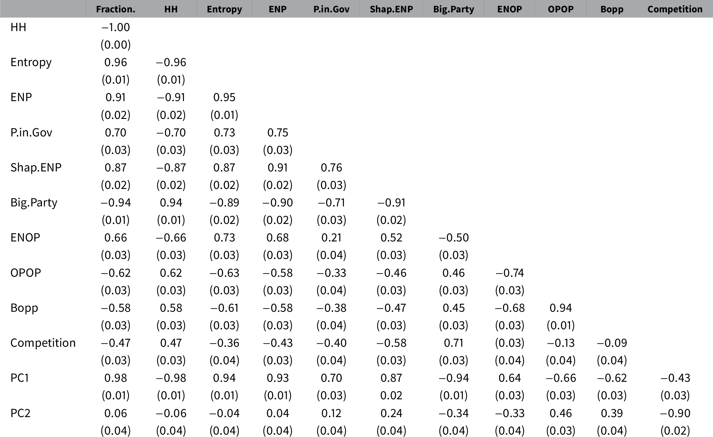
Note: Computed correlation using Pearson method with pairwise deletion. Standard errors are in parentheses. Abbreviations: Fraction, Fractionalization Index; HH, Herfindahl–Hirschman Index; Entropy, entropies; ENP, effective number of parties; P.in Gov, number of parties in the government; Shap.ENP, effective number of parties (Shapley); Big Party, size of the biggest party over the size of the legislature; ENOP, effective number of opposition parties; OPOP, the difference between the first and the second biggest opposition parties over the size of the legislature; BOPP, size of the biggest opposition party over the size of the legislature; Competition, size difference between the biggest and the second biggest parties over the size of the legislature. PC1: Dimension 1, Sizes of the two biggest parties. PC2: Dimension 2, Competition between the biggest and the second biggest parties.
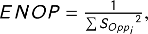
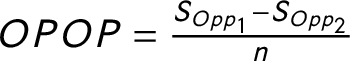
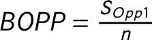
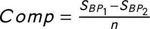
To measure the competition within the party system, we might calculate indices that measure the structure of the opposition. The concentration of the opposition could be measured similarly to the party system size. This notion has been discussed previously in a few studies (Maeda Reference Maeda2010, Reference Maeda2015). However, very few political science research have used these measures. The Effective Number of Opposition Parties (ENOP) is calculated the same way as the ENP suggested by Laakso and Taagepera (Reference Laakso and Taagepera1979), except I calculate the measure only for the opposition parties. The Difference Between the Biggest and the Second Biggest Opposition Parties (OPOP) measures the competition between the biggest and the second biggest opposition parties. I normalize the difference between the seat shares of the two biggest opposition parties by the number of total available legislative seats within a country. The Size of the Biggest Opposition Party (BOPP) measures the size of the biggest party in the opposition also normalized with the number of the legislative seats. Finally, I calculate the Competition, which is the seat share difference between the biggest and the second biggest parties normalized with the number of legislative seats.Footnote 15 The last two rows of Table 2 show that the opposition measures and the competition measure relate both to PC2 and to PC1 while the party system size measures are closely related to only PC1. The only exception is the size of the Biggest Party (Big Party), which seems to be somewhere in between the opposition measures and the party system size measures. This makes sense because it is possible that the biggest party in the party system is not a government party but an opposition party.

Figure 7 Measures on the PC dimensions. Notes: The plot shows how party system size measures relate to each other and the two first dimensions of the PCA. PC1: Dimension 1, Sizes of the two biggest parties. PC2: Dimension 2, Competition between the biggest and the second biggest parties. Abbreviations: HH, Herfindahl–Hirschman Index; Fract, Fractionalization Index; Entropy, entropies; ENP, effective number of parties; P.in Gov, number of parties in the government; Shap.ENP, effective number of parties (Shapley); Big Party, size of the biggest party over the size of the legislature; ENOP, effective number of opposition parties; OPOP, the difference between the first and the second biggest opposition parties over the size of the legislature; BOPP, size of the biggest opposition party over the size of the legislature; Competition, size difference between the biggest and the second biggest parties over the size of the legislature.
I also plot the indices on PC Dimensions 1 and 2 to show how the indices relate to these dimensions (Figure 7). First, I regress each index on the PC1 and PC2 dimensions and plot the coefficients.Footnote 16 Figure 7a also shows that most of the indices that the current scholarship uses are closer to Dimension 1 while opposition concentration measures are closer to Dimension 2. Figure 7a offers a way in which we can decide between measures with multicriteria decision-making process, as the curve can serve as the basis of a pareto-optimization. The more we would like to take into account competition between the parties with our measure and less the number of parties, the closer index we should choose to Dimension 2. Alternatively, if our theory calls for the size of the party system, we can choose one of the variables close to Dimension 1. Similarly, we can evaluate how the measures relate to the PC dimensions by using the Sum of Ranking Differences method. First, I calculate how the country-years are ranked on the PC1 and PC2 dimensions. Then, I calculate how the various country-years are ranked by the indices. Finally, I deduct the PC1 and PC2 rankings from the rankings of the measures. The sum of the differences is the Sum of Ranking Differences. The low values indicate that the index is close to the dimension, and higher values indicate that the index is far. Since the PC method is nondirectional, I repeat the process with inverse ranking as well to find the measure that is the closest to the PCA solution. I find that the HH followed by the Fractionalization and ENP (identical in their ranking) are the closest to the Dimension 1’s ranking of country-years. This result shows that neither transformation of the HH changes the measure in a meaningful way. At the same time, the measure Competition is the closest to Dimension 2 followed by OPOP, ENOP, and BOPP (Héberger and Kollár-Hunek Reference Héberger and Kollár-Hunek2011; Bajusz, Rácz, and Héberger Reference Bajusz, Rácz and Héberger2015). I plot the normalized results against the theoretical distribution of random rankings in Figure 7b.
6 Conclusion
In this paper, I conducted a PCA of data comprising party seat shares of 17 European countries from 1970 to 2013. I argued that although the data were compositional, the best choice for understanding the underlying structure of the party system data was to examine the untransformed dataset. The PCA revealed that the absolute sizes of the biggest parties and the relative sizes of the two biggest parties (i.e., the level of competition between the two biggest parties) were the two most important features that differentiated party systems from each other in Europe during the study period.
I suggested several applications of this method to improve the general understanding of party systems and how they can be measured. The first two dimensions that the method recovered could be used to track party system changes within countries. I also conducted a PCA on party vote shares and demonstrated how electoral party system changes could be compared to legislative party system changes with the proposed method.
Second, PCA can help users of party system typologies and indices to understand the measures that they use. A comparison of the PCA results with the results produced using Rokkan’s (Reference Rokkan1970) typology showed that the PCA grouped countries together that Rokkan had classified as belonging to the same groups. With the help of the PCA, I showed how the typologies could be used in quantitative studies. I classified countries that Rokkan did not classify and showed that the PCA method can automatically sort each country by year in the dataset into a “type.”
Finally, I compared the results of the PCA to some traditional party system size indices that many researchers currently use. This comparison revealed that most of these indices were highly correlated with each other and with Dimension 1 (i.e., size of the biggest two parties). Empirical analysts should be aware that the indices they use frequently are highly correlated with other indices that could be conceptually different yet still produce the outcomes that they are interested in. In addition, if possible, they should avoid using more than one of these indices within the same model. Furthermore, I suggested that we might want use other indices if we wanted to measure the competitiveness of a party system. I calculated some indices that measure opposition concentration and competition, and showed that these relate to Dimension 2. I proposed that these may be better suited for measuring the competitiveness of party systems than the traditional party system size indices.
Acknowledgments
The author would like to thank Mark S. Handcock, Chad Hazlett, and Nicolas Christou at the University of California, Los Angeles, who supported this project. She would also like to thank Jeffrey B. Lewis and Bang Quan Zheng at the University of California, Los Angeles, and Ingrid D. Mauerer at the University of Barcelona for their valuable input. She would also like to thank Michael F. Thies, Kathleen Bawn, Thomas Schwartz, and Michael Chwe at the University of California, Los Angeles, and Sona N. Golder at Penn State University for their advise on parties and party systems. She would also like to thank the panel audience at the PSA Political Methodology Conference 2018 in Essex for their helpful comments, as well as the Comparative Political Science student association at the University of California, Los Angeles. She would also like to thank Jeff Gill, the Editor, and the three anonymous reviewers for their highly valuable comments.
Data Availability Statement
For Dataverse replication materials, see Magyar (Reference Magyar2021).
Supplementary Material
For supplementary material accompanying this paper, please visit https://doi.org/10.1017/pan.2021.21.


 Open access