


Introduction
Ediacara-type fossil assemblages, known from nearly 40 million years before the Cambrian explosion of skeletonized metazoans, include a diverse suite of globally distributed, exceptionally preserved, macroscopic, morphologically disparate soft-bodied organisms that are largely absent from the post-Ediacaran record (Narbonne Reference Narbonne2005; Xiao and Laflamme Reference Xiao and Laflamme2009; Droser and Gehling Reference Droser and Gehling2015). Many constituents of Ediacara-type assemblages are interpreted as belonging to whole-group metazoa (Droser and Gehling Reference Droser and Gehling2015; Bobrovskiy et al. Reference Bobrovskiy, Hope, Ivantsov, Nettersheim, Hallmann and Brocks2018), although there is considerable uncertainty regarding which specific lineages are represented (MacGabhann Reference MacGabhann2014). The ecological structure of Ediacaran paleocommunities is enigmatic: they show some structural similarities to younger benthic paleocommunities (Clapham et al. Reference Clapham, Narbonne and Gehling2003; Droser and Gehling Reference Droser and Gehling2015; Laflamme and Darroch Reference Laflamme and Darroch2015), but differ in the absence or near absence of predation and infaunalization and the limited number of motile taxa (Droser and Gehling Reference Droser and Gehling2015; Chen et al. Reference Chen, Chen, Zhou, Yuan and Xiao2018). Understanding the ecology of Ediacarans is additionally complicated by the unusual mode of preservation of most Ediacaran assemblages as casts and molds in early-cemented sandstones (Tarhan et al. Reference Tarhan, Hood, Droser, Gehling and Briggs2016).
One of the best-studied Ediacaran assemblages is found at the Nilpena National Heritage Site, west of the Flinders Ranges in South Australia. Over the past 16 years, 34 beds in the Ediacara Member of the Rawnsley Quartzite have been excavated and mapped, exposing thousands of fossils, including many new taxa (Droser et al. Reference Droser, Gehling, Tarhan, Evans, Hall, Hughes, Hughes, Dzaugis, Dzaugis, Dzaugis and Rice2017). One of the most striking observations to emerge from this work is that successive beds exhibit little sedimentological variation but substantial variation in diversity–abundance structure (Droser and Gehling Reference Droser and Gehling2015; Droser et al. Reference Droser, Gehling, Tarhan, Evans, Hall, Hughes, Hughes, Dzaugis, Dzaugis, Dzaugis and Rice2017). If this variability is truly unusual in the context of younger assemblages, it might offer insight into the ecology and/or taphonomy of benthic ecosystems before the advent of widespread motility, predation, and bioturbation in the Phanerozoic.
Here we use a compilation of fossil and modern marine benthic ecological data sets, each consisting of multiple collections from the same local area, time interval, and habitat, to quantitatively compare the variability of Ediacaran faunal assemblages to that of younger fossil and modern benthic assemblages. We examine both the partitioning of diversity into within-collection (α) and between-collection (β) components and the pairwise dissimilarities among collections within each data set.
Data
Ediacaran Data Sets
The Ediacara Member of the Rawnsley Quartzite, outcropping in the Flinders Ranges of South Australia, is host to a diverse array of taxa comprising a wide variety of morphologies (Droser and Gehling Reference Droser and Gehling2015; Droser et al. Reference Droser, Gehling, Tarhan, Evans, Hall, Hughes, Hughes, Dzaugis, Dzaugis, Dzaugis and Rice2017). The National Heritage Ediacara fossil site at Nilpena Station provides the opportunity to examine successive bedding planes from two fossiliferous facies representing distinct habitats: (1) oscillation-rippled sandstone facies, which is interpreted to have been deposited between fair-weather and storm wave base, and (2) planar-laminated and rip-up sandstone facies, which is interpreted to represent sub–wave base upper canyon fill deposition (Droser et al. Reference Droser, Gehling, Tarhan, Evans, Hall, Hughes, Hughes, Dzaugis, Dzaugis, Dzaugis and Rice2017; Tarhan et al. Reference Tarhan, Droser, Gehling and Dzaugis2017). Beds are laterally discontinuous and range from millimeters to about 10 cm in thickness. We included all beds for which at least 50 individual fossils have been counted (23 from the oscillation-rippled sandstone facies and 4 from the planar-laminated sandstones facies). These two data sets include ~28 taxa in total (Supplemental Data File 1). All beds are from within a very small geographic region (maximum distance between samples <500 m) and in many cases are directly superposed. Fronds and associated stalks and holdfasts are an important component of the Nilpena assemblages, but because they are commonly shredded and incomplete, it is not always possible to identify them to genus. All fronds are therefore grouped together in a single “genus.” This is conservative, in that it will tend to reduce, rather than inflate, apparent faunal differences between collections. Macrofossil taxa that have been interpreted as algal, such the informally named “Bundle of Filaments” (Xiao et al. Reference Xiao, Droser, Gehling, Hughes, Wan, Chen and Yuan2013) were excluded.
The only other Ediacaran assemblage that has been comparably studied at the bed scale is the substantially older (~570 Ma) and much deeper-water Mistaken Point biota of Newfoundland. Clapham et al. (Reference Clapham, Narbonne and Gehling2003) censused seven fossiliferous bedding planes in the slope-basinal siliciclastic sediments of the Conception and St. John's Groups. These formations span a significant range of time and of depositional environments (Narbonne et al. Reference Narbonne, Dalrymple, Wood, Gehling and Clapham2003; Ichaso et al. Reference Ichaso, Dalrymple and Narbonne2007). Consequently, to reduce the potential impact of evolutionary turnover and habitat turnover on bed-to-bed faunal variation, for this analysis we include only the four beds from the Mistaken Point Formation.
Phanerozoic Fossil Data Sets
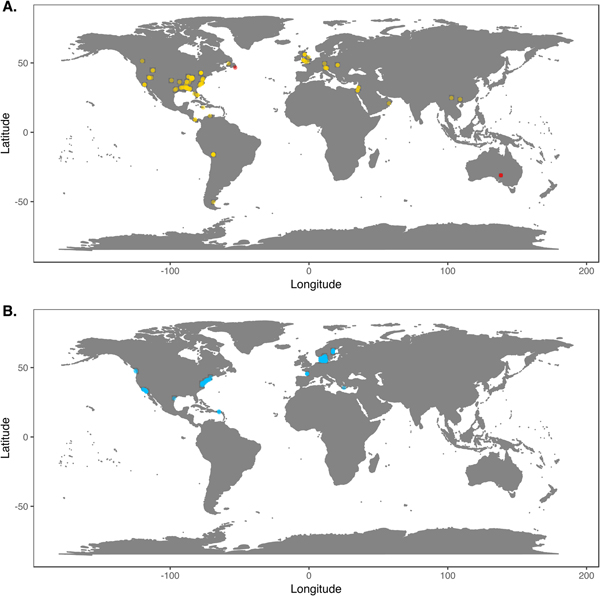
We downloaded Phanerozoic marine body fossil occurrence records from the Paleobiology Database on March 3, 2018 (Supplementary Data File 2; see Supplementary Appendix 1 for download criteria and metadata). In our analyses we included only collections from level-bottom, soft substrate environments (reefs, bioherms, and buildups excluded). We further limited the analysis to collections made for paleoecological studies in which abundance counts were recorded for all reported taxa. To ensure that our data sets were ecologically comparable to the exclusively benthic Ediacaran data sets, we excluded nektonic and planktonic macrofaunal groups such as ammonites; graptolites; and fish and microfossil groups such as conodonts, radiolarians, and foraminifera. We included only collections consisting of at least 50 individuals representing at least two genera and, to ensure that collecting effort was not focused on a single taxon, at least two classes. We grouped collections into assemblage data sets if they were from the same formation and member, the same stratigraphic stage, the same lithofacies and depositional environment, and within 0.01° latitude and 0.01°longitude of one another (maximum distance between collections of ~1.6 km). We excluded collections with poorly resolved lithological descriptors (e.g. “indet. siliciclastic”) to ensure that all collections in a data set came from genuinely similar lithofacies. The final Phanerozoic fossil database consists of 170 local data sets ranging from middle Cambrian to Pliocene in age. The majority include only skeletonized taxa, but two data sets, from the early Cambrian Maotianshan Shale (Zhao et al. Reference Zhao, Caron, Bottjer, Hu, Yin and Zhu2013; Supplementary Data File 3) and the middle Cambrian Burgess Shale (Caron and Jackson Reference Caron and Jackson2008), include diverse soft-bodied taxa. Fossil data sets are globally distributed, but Europe and North America are disproportionately represented (Fig. 1A).

Figure 1. A, Locations of fossil data sets included in analyses. Light points are Phanerozoic data sets, dark points in South Australia and Newfoundland are Ediacaran data sets. B, Locations of modern data sets included in analyses.
Modern Data Sets
We downloaded benthic data sets from a variety of data sources, with the majority coming from the Ocean Biogeographic Information System (OBIS) and its regional affiliates (Supplementary Data File 4) and from the U.S. Environmental Protection Agency's Environmental Monitoring and Assessment (EMAP) program and National Coastal Assessment (Supplementary Data File 5). We included only collections gathered by grab sampling or box-coring of level-bottom, soft-substrate environments in which all or most benthic macrofauna and megafauna were identified at least to genus and counted. We used two criteria, substrate type and depth, to assign collections to habitat types roughly comparable to facies in the sedimentary record. Substrate data are available for all EMAP collections but not for all OBIS collections, so for European data sets we intersected collection coordinates with a benthic substrate map of European waters (Populus et al. Reference Populus, Vasquez, Albrecht, Manca, Agnesi, Al Hamdani, Andersen, Annunziatellis, Bekkby, Bruschi, Doncheva, Drakopoulou, Duncan, Inghilesi, Kyriakidou, Lalli, Lillis, Mo, Muresan, Salomidi, Sakellariou, Simboura, Teaca, Tezcan, Todorova and Tunesi2017). We grouped collections into local data sets if they were from the same source and collected during the same year using the same protocols, from the same substrate type, the same 5 m depth bin, and from within 0.01° latitude and 0.01°longitude of one another. As with the fossil data, we only included data sets consisting of two or more collections with at least 50 individuals in each collection. The final modern database consisted of 265 local data sets, primarily from northern Europe and the United States (Fig. 1B). Whereas in the fossil record there is an almost unavoidable trade-off between increasing geographic scale of analysis and decreasing temporal resolution (Jablonski Reference Jablonski2000), modern collections provide the opportunity to examine the relationship between increasing geographic distance and degree of faunal dissimilarity in a single geological instant. Quantifying this relationship while holding depth and substrate type constant can contextualize within-facies bed-to-bed faunal dissimilarities in the fossil record. For these comparisons, modern data sets were defined as above, but without imposing geographic limitations. All data sets used are available for download at the Harvard Dataverse Repository (https://dataverse.harvard.edu/dataset.xhtml?persistentId=doi:10.7910/DVN/JLQRXP).
Methods
All data sets were analyzed at the genus level due to inconsistent reporting of species identities in both fossil and modern databases and variation in taxonomic practices across different groups and time intervals. This is conservative, in that it can only act to reduce, rather than inflate, apparent faunal differences among the collections in a data set. Diversity partitioning and pairwise sample dissimilarity analyses were carried out using the ‘vegan’ R package. Because all diversity metrics are strongly influenced by variation in sample size (Beck et al. Reference Beck, Holloway and Schwanghart2013), we standardized sample sizes by subsampling, without replacement, 50 individuals from each collection. We calculated mean α and multiplicative β diversity (Jost Reference Jost2007; Baselga Reference Baselga2010) for each subsampled data set with the multipart function, using a Hill's number (q) of 1 so that diversity estimates are equivalent to linearized Shannon-Wiener diversity and reflect both the evenness and richness components of diversity (Jost Reference Jost2007). We determined the mean “expected” β diversity of each subsampled data set by taking the mean β diversity from 100 random draws of N samples of 50 individuals from the pooled (γ) distribution, where N is the number of collections in the data set (random draws were done by setting the “nsimul” parameter in multipart to 100). We then calculated “excess” β diversity by subtracting expected from observed β diversity values in each subsampled data set. Because there is considerable debate over the properties of different β-diversity metrics, we also calculated β diversity for each subsampled data set as the mean Bray-Curtis dissimilarity between all subsampled collections and the data set centroid. All of the above procedures were repeated 100 times for each data set to place 95% confidence intervals on diversity estimates.
To quantify the relationship between β diversity and geographic distance within modern benthic habitats and compare it with bed-to-bed β diversity in fossil assemblages, we calculated pairwise Bray-Curtis distances among all collections within both modern and fossil data sets. In the modern data sets, we calculated the median dissimilarity between collection pairs in each log2 distance bin. Annotated code for reproducing our analyses is in Supplemental File 1.
Results
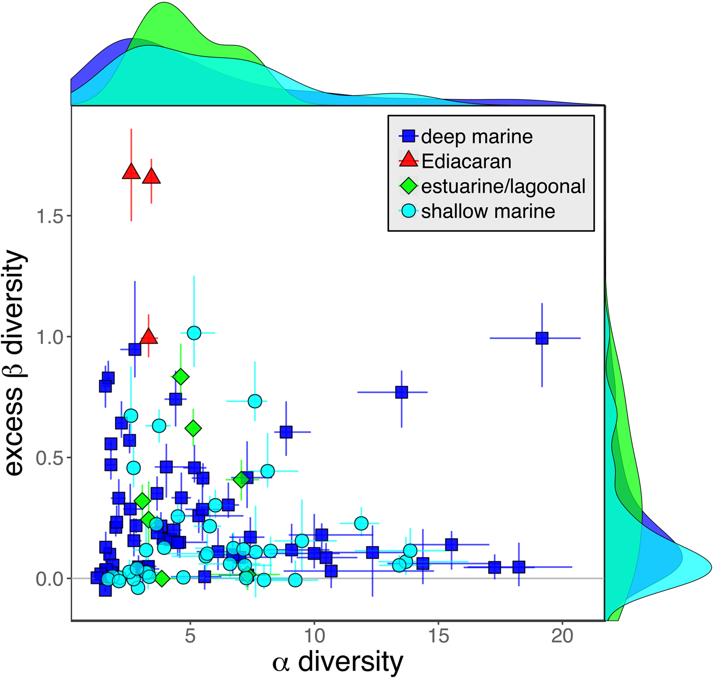
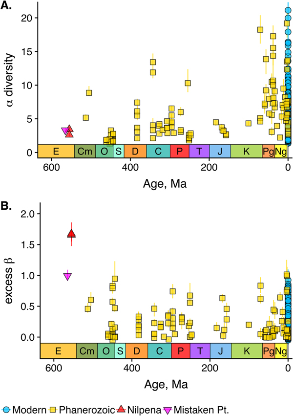
As is expected given the absence of soft-bodied taxa in most fossil assemblages, Phanerozoic fossil data sets have significantly lower α diversity than modern data sets (two-sided Wilcox test p << 0.001, two-sided Kolmogorov-Smirnov test p << 0.001) (Fig. 2). However, excess β distributions of fossil and modern data sets do not differ significantly (two-sided Wilcox test p = 0.22, two-sided Kolmogorov-Smirnov test p = 0.47). Ediacaran data sets exhibit relatively low α diversity but high excess β compared with both the Phanerozoic and modern fossil data sets (Fig. 2). Ediacaran data sets have α diversities near or below the modal value for Phanerozoic and modern data sets, but excess β values that are very high relative to Phanerozoic and modern data sets (97th to 100th percentile). Within the Phanerozoic, there is a trend toward higher α diversity, consistent with previous analyses (Bambach Reference Bambach1977; Bush and Bambach Reference Bush and Bambach2004), but no consistent trend in excess β (Fig. 3).
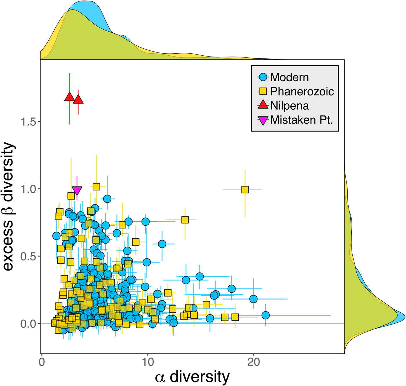
Figure 2. Mean α versus excess β diversity for all Ediacaran, Phanerozoic, and modern assemblages. Diversity is expressed in species equivalents using a Hill number of 1 and thus reflect both the richness and evenness components of diversity (Jost Reference Jost2007; Baselga Reference Baselga2010). Bars indicate the 95% confidence interval for each data set, based on 100 subsampling iterations. Data sets with y confidence intervals overlapping zero do not have β diversity significantly exceeding that expected from random sampling of the pooled vector of genus abundances. Marginal plots show proportional frequency distributions for Phanerozoic and modern data sets. Data sets are here defined as sets of collections collected from the same substrate type and depth range (modern) or formation and facies (fossil) by the same set of workers within an ~1 km2 area (within a single year for modern data sets).

Figure 3. A, αα-diversity component of fossil data sets through time. B, Excess β-diversity component of fossil data sets through time (Nilpena points are overplotted). Confidence intervals as in Fig. 1. E, Ediacaran; Cm, Cambrian; O, Ordovician; S, Silurian; D, Devonian; C, Carboniferous; P, Permian; T, Triassic; J, Jurassic; K, Cretaceous; Pg, Paleogene; Ng, Neogene.
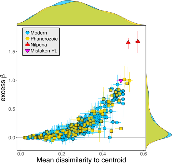
Because it is expressed as a multiple of mean α diversity, β diversity (and excess β) is more likely to reach very high values when mean α diversity is low (Veech and Crist Reference Veech and Crist2010), as it generally is for Ediacaran data sets. However, excess β values of Ediacaran data sets are high, even relative to Phanerozoic and modern data sets with comparable mean α diversity (Fig. 2). The β diversity of a given data set is also partially dependent on the number of collections examined (Marion et al. Reference Marion, Fordyce and Fitzpatrick2017). The number of collections in Ediacaran data sets ranges from 4 (Nilpena planar-laminated sandstone facies and Mistaken Point Formation) to 19 (Nilpena oscillation-rippled sandstone facies), but excess β values in all three cases are high relative to other fossil data sets with comparable numbers of collections (Fig. 4), individuals (Fig. 5), and genera (Fig. 6). This result is not method dependent, as Ediacaran β values are also very high when measured as mean Bray-Curtis dissimilarity from the data set centroid (Fig. 7).

Figure 4. Excess β diversity versus log number of collections in each data set. Confidence intervals and marginal frequency distributions as in Fig. 2.
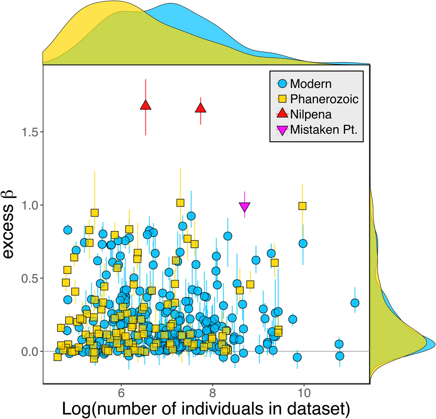
Figure 5. Excess β diversity versus log number of individuals in each data set. Confidence intervals and marginal frequency distributions as in Fig. 2.
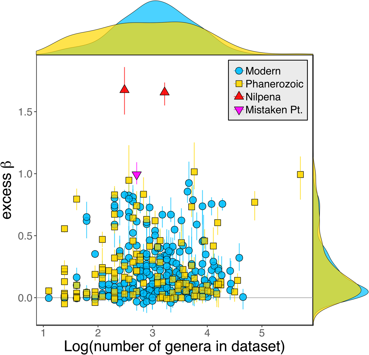
Figure 6. Excess β diversity versus log number of genera in each data set. Confidence intervals and marginal frequency distributions as in Fig. 2.

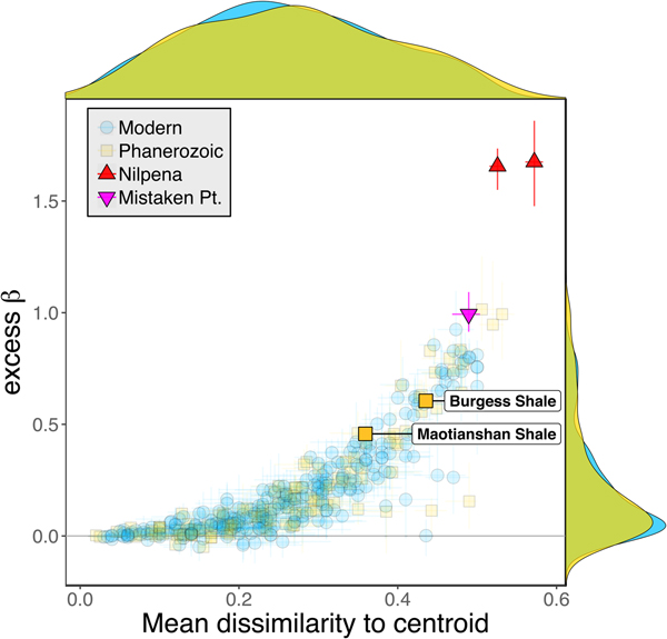
Figure 7. Excess β diversity of data sets versus mean Bray-Curtis dissimilarity from the data set centroid. Confidence intervals and marginal frequency distributions as in Fig. 2.
We aggregated modern collections into local data sets at the same geographic scale as fossil collections (within ~1 km of each other). However, this choice of spatial scale is somewhat arbitrary, given that the fossil data sets represent far greater time spans. Plotting the distance–decay of faunal similarity within modern habitats, as measured by pairwise Bray-Curtis distance, provides a richer framework for comparing the spatial variation observed in a single time slice with the temporal variation observed in the fossil record (Fig. 8). The distribution of mean pairwise distances between beds in Phanerozoic fossil data sets suggests that they typically capture a range of faunal variation comparable to that seen over meters to kilometers in modern shallow, benthic ecosystems. In contrast, Ediacaran data sets exhibit mean pairwise distances more comparable to those observed over tens to hundreds of kilometers in modern ecosystems.
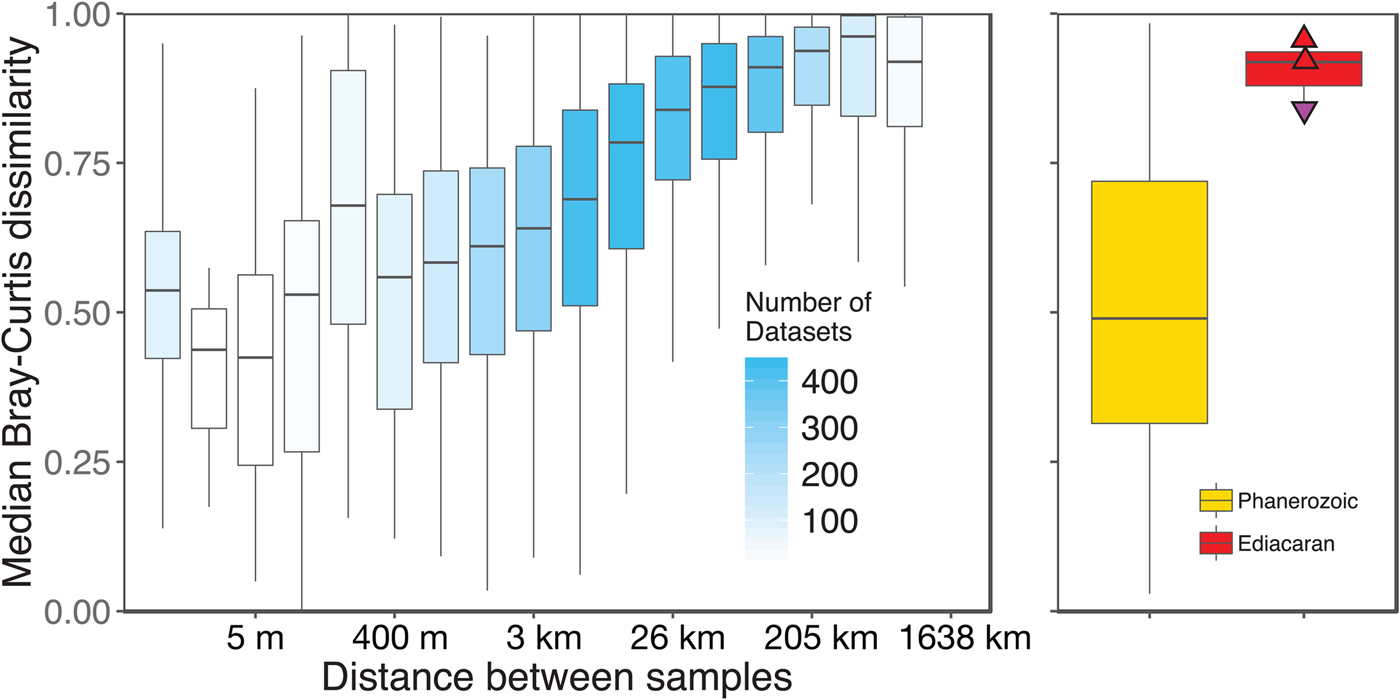
Figure 8. Median pairwise Bray-Curtis dissimilarities within log2 distance bins for all modern data sets compared with median pairwise Bray-Curtis dissimilarities of Ediacaran data sets and Phanerozoic data sets. Box-and-whisker plots show median (horizontal bar) interquartile range (IQR) (boxes), and range of values within 1.5*IQR on either side of the median (whiskers). For modern data sets (left/blue), shading of boxes indicates number of data sets included. Points on Ediacaran distribution as in Figs. 2–7. Phanerozoic data sets span a wide range of median pairwise dissimilarity values but are most comparable to modern values at small to intermediate distances, whereas Ediacaran values are most comparable to those observed at distances of tens to hundreds of kilometers in modern data sets. Modern data sets are here defined as sets of collections collected from the same substrate type and depth range by the same set of workers within a single year.
Discussion
Unrecognized environmental or temporal gradients are a potential source of error in our analyses. The Ediacaran data sets were field collected with associated sedimentological data, making it possible to confidently differentiate facies and examine only within-habitat β diversity. We were as stringent as possible in limiting habitat variation in fossil and modern data sets with the data available, but it is possible that some data sets cover significant gradients in depth and/or substrate type. In addition, although we restricted the temporal coverage of fossil data sets as much as possible given available chronostratigraphic constraints, in some data sets there may still be some temporal turnover in the composition of the species pool. However, this cannot explain the low β diversity of Phanerozoic and modern data sets, as environmental or temporal gradients can only inflate apparent β diversity by mixing samples from different habitats or time intervals. Ediacaran organisms are less well understood than younger taxa, and so it is possible that they are taxonomically undersplit, but this would tend to reduce Ediacaran β-diversity estimates rather than inflate them.
Accepting that the pattern is genuine and not an artifact of how collections are aggregated into data sets, three non–mutually exclusive hypotheses can be formulated to explain the exceptional bed-to-bed variability of Ediacaran assemblages. First, it is possible that Ediacaran assemblages represent different depositional environments, with different gradients and disturbance dynamics, than other assemblages. Second, Ediacaran assemblages may be less spatiotemporally averaged than younger fossil assemblages due to the absence of skeletonization and bioturbation. Finally, Ediacara-type faunas may have been genuinely more variable in space and time than younger benthic ecosystems.
Available data provide mixed support for the first hypothesis. Inferred depositional environments of Ediacaran data sets analyzed here range from nearshore (Nilpena) to outer slope (Mistaken Point), and nothing in the sedimentology of these units suggests that they represent unusual environments. Although it has been suggested that the Ediacara Member includes a range of terrestrial environments (Retallack Reference Retallack2013), this interpretation has been widely rejected (Callow et al. Reference Callow, Brasier and McIroy2013; Xiao et al. Reference Xiao, Droser, Gehling, Hughes, Wan, Chen and Yuan2013; Tarhan et al. Reference Tarhan, Droser and Gehling2015a). The Ediacara Member may represent a lagoonal or estuarine setting, but Ediacaran data sets exhibit elevated variability even when compared with fossil data sets from lagoonal and estuarine settings (Fig. 9). Dissolved oxygen levels in shallow waters were probably lower in the Ediacaran than during most of the Phanerozoic (Lyons et al. Reference Lyons, Reinhard and Planavsky2014; Sperling et al. Reference Sperling, Wolock, Morgan, Gill, Kunzmann, Halverson, Macdonald, Knoll and Johnston2015), but the typically low faunal variability of modern low-oxygen settings (Levin Reference Levin2003) suggests that low oxygen is unlikely to explain the unusual variability of Ediacaran assemblages. However, there is growing evidence for strongly fluctuating redox conditions in some Ediacaran-aged successions (Bowyer et al. Reference Bowyer, Wood and Poulton2017), and such fluctuations would be expected to generate highly variable faunal assemblages within a single facies.
Mode of preservation and degree of time averaging are almost certainly an important component of the exceptional variability of Ediacaran assemblages. Phanerozoic data sets consist primarily of shelly fossils in bioturbated sediments and are consequently relatively time-averaged (Kidwell and Daniel Reference Kidwell, Daniel, Allison and Briggs1991). Because they predate the advent of extensive bioturbation, Ediacaran assemblages are expected to have higher temporal resolution. Time averaging of shelly fossils acts to transfer diversity from β to α levels (Finnegan and Droser Reference Finnegan and Droser2008; Tomašových and Kidwell Reference Tomašových and Kidwell2009), potentially obscuring the original patchiness of benthic communities. The faunal variability of Ediacaran assemblages compared with that of the Phanerozoic fossil record may thus be, at least in part, a consequence of their high temporal resolution—they may offer snapshots of larval settlement patterns (Droser and Gehling Reference Droser and Gehling2008; Mitchell et al. Reference Mitchell, Kenchington, Liu, Matthews and Butterfield2015) and successional dynamics (Clapham et al. Reference Clapham, Narbonne and Gehling2003; Coutts et al. Reference Coutts, Gehling and García-Bellido2016; Reid et al. Reference Reid, García-Bellido, Payne, Runnegar and Gehling2017) that occur on timescales too short to be captured by the time-averaged Phanerozoic shelly record.
Some support for this hypothesis comes from comparison with the Cambrian Burgess Shale and Maotianshan Shale, the only other soft-bodied Lagerstätte for which sufficient paleoecological data are available (Caron and Jackson Reference Caron and Jackson2008; Zhao et al. Reference Zhao, Caron, Bottjer, Hu, Yin and Zhu2013). Both of these data sets exhibit relatively high β diversity (Fig. 10). Although direct comparison is difficult, because the Cambrian assemblages formed in relatively deep-water habitats, the generally high β diversity of Ediacaran and Cambrian Lägerstatten suggests that data sets with high temporal resolution do indeed tend to preserve greater bed-to-bed variation in diversity–abundance structure. Thus, in addition to providing unusual windows into organismal morphology and paleocommunity composition, some Lagerstätten may also preserve exceptional records of paleoecological dynamics. We also note that although there is little trend in the mean excess β value of Phanerozoic shelly fossil data sets, some of the highest observed values occur in Ordovician–Silurian data sets (Fig. 3). This is consistent with suggestions that, because they precede the post-Silurian advent of modern bioturbation intensities (Tarhan et al. Reference Tarhan, Droser, Planavsky and Johnston2015b), some early Paleozoic benthic shelly fossil assemblages may preserve a higher-resolution paleoecological record than younger assemblages (Bambach et al. Reference Bambach, Droser, Sepkoski, Einsele, Ricken and Seilacher1991).

Figure 10. Excess β diversity of data sets versus mean Bray-Curtis dissimilarity from the data set centroid, with the two Cambrian Lagerstätte highlighted. Confidence intervals and marginal frequency distributions as in Fig. 2.
It is likely that the unusual variability of Ediacaran assemblages also reflects some key ecological differences compared with younger benthic paleocommunities. The most important of these may be the rarity of motile taxa in Ediacaran assemblages, which would be expected to lead to patchier communities strongly influenced by dispersal limitations. One of the few motile taxa in the Nilpena assemblages, Dickinsonia, occurs on nearly all beds in both facies (Droser et al. Reference Droser, Gehling, Tarhan, Evans, Hall, Hughes, Hughes, Dzaugis, Dzaugis, Dzaugis and Rice2017). Only the holdfast form genus Aspidella shares a similar distinction (Droser et al. Reference Droser, Gehling, Tarhan, Evans, Hall, Hughes, Hughes, Dzaugis, Dzaugis, Dzaugis and Rice2017), and it is unknown how many different frond taxa Aspidella might in fact represent (Gehling et al. Reference Gehling, Narbonne and Anderson2000).
Another factor that may help to explain the high faunal patchiness of Ediacaran assemblages is the inferred presence of multiple reproductive and dispersal modes. A number of Ediacaran taxa exhibit evidence of planktonic dispersal (Clapham et al. Reference Clapham, Narbonne and Gehling2003; Droser and Gehling Reference Droser and Gehling2008; Darroch et al. Reference Darroch, Laflamme and Clapham2013; Mitchell et al. Reference Mitchell, Kenchington, Liu, Matthews and Butterfield2015), but some may also have engaged in asexual clonal reproduction via stolons (Mitchell et al. Reference Mitchell, Kenchington, Liu, Matthews and Butterfield2015), a trait that would lead to patchy species distributions. Patchiness may also reflect successful colonization related to organism height and dispersal (Mitchell and Kenchington Reference Mitchell and Kenchington2018).
Finally, competitive interactions may have had a stronger influence on paleocommunity composition in the Ediacaran than in younger ecosystems. Relative abundance distributions suggest that at least some Ediacaran assemblages included taxa that competed with one another for resources (Darroch et al. Reference Darroch, Laflamme and Wagner2018). Ediacaran ecosystems also lacked widespread predation and bioturbation—−processes that exert a powerful influence on the structure of younger benthic ecosystems (Erwin and Tweedt Reference Erwin and Tweedt2012) and may act to reduce the importance of competition (Stanley Reference Stanley2008). In their absence, then, competitive interactions could have had a stronger influence on community structure and composition. Competition-dominated ecosystems are generally predicted to be characterized by low α diversity and high β diversity (Hautmann Reference Hautmann2014), a prediction that is consistent with the patterns we observe.
Conclusions
Here we have demonstrated that, compared with the Phanerozoic fossil record, Ediacaran assemblages are characterized by unusual bed-to-bed variability in faunal diversity and abundance. Comparisons between fossil and modern benthic assemblages are complicated by the limited spatial scale of the former and the limited temporal scale of the latter, but whereas the faunal variability of Phanerozoic shelly fossil data sets is consistent with relatively local-scale variation in modern benthic habitats, Ediacaran assemblages exhibit variability typically observed only over much greater distances in modern habitats. Additional high-resolution field studies of Ediacaran and Phanerozoic fossil assemblages and modeling exercises are required to determine whether this unusual variability primarily reflects differences in taphonomy, community ecology, or a combination of the two.
Acknowledgments
We thank R. and J. Fargher for access to the National Heritage Ediacara fossil site Nilpena on their property, acknowledging that this land lies within the Adnyamathanha Traditional Lands. We thank M. Clapham, L. Tarhan, and A. Tomašových for helpful discussions, and M. Laflamme and an anonymous reviewer for constructive reviews. This work was funded by the NASA Exobiology Program (NASA grant NNX14AJ86G to M.L.D.); the Australian Research Council (grant DP0453393 to J.G.G.); the National Geographic Society (grant 9476-14 to M.L.D.); the Ediacaran Foundation; the South Australian Museum Waterhouse Club; the University of California, Riverside; Beach Energy (M.L.D. and J.G.G.); and a David and Lucile Packard Fellowship (S.F.). Some of the data described in this article were produced by the U.S. Environmental Protection Agency through its Environmental Monitoring and Assessment Program (EMAP), http://www.epa.gov/emap. Information contained here has been derived from data made available under the European Marine Observation Data Network (EMODnet) Seabed Habitats project (www.emodnet-seabedhabitats.eu), funded by the European Commission's Directorate-General for Maritime Affairs and Fisheries (DG MARE). This is Paleobiology Database contribution number 327.


 Open access