


Introduction
Origination and Extinction across Space
Origination and extinction are two of the most fundamental processes in evolution, structuring taxonomic diversity across space and time (Allen and Gillooly Reference Allen and Gillooly2006; Jablonski Reference Jablonski2008; Schluter and Pennell Reference Schluter and Pennell2017). Understanding spatial variation in origination and extinction can help to unravel the mechanisms underlying macroevolutionary patterns, such as latitudinal diversity gradients (Mittelbach et al. Reference Mittelbach, Schemske, Cornell, Allen, Brown, Bush, Harrison, Hurlbert, Knowlton, Lessios, McCain, McCune, McDade, McPeek, Near, Price, Ricklefs, Roy, Sax, Schluter, Sobel and Turelli2007; Mannion et al. Reference Mannion, Upchurch, Benson and Goswami2014; Powell et al. Reference Powell, Moore and Smith2015; Schluter and Pennell Reference Schluter and Pennell2017; Saupe et al. Reference Saupe, Myers, Peterson, Soberón, Singarayer, Valdes and Qiao2019; Meseguer and Condamine Reference Meseguer and Condamine2020), and provide deeper insight into biotic crises and radiations (Jablonski Reference Jablonski2008; Saupe et al. Reference Saupe, Hendricks, Portell, Dowsett, Haywood, Hunter and Lieberman2014; Kocsis et al. Reference Kocsis, Reddin and Kiessling2018; Reddin et al. Reference Reddin, Kocsis and Kiessling2019; Flannery-Sutherland et al. Reference Flannery-Sutherland, Silvestro and Benton2022).
Although methods have been developed for estimating global origination and extinction rates from the fossil record, no framework exists for applying these methods to restricted spatial regions. Raw evolutionary rates have been calculated previously within latitude bands (e.g., Powell et al. Reference Powell, Moore and Smith2015; Song et al. Reference Song, Huang, Jia, Dai, Wignall and Dunhill2020), but this approach does not take into account variation in the sampling completeness of the fossil record (Benson and Upchurch Reference Benson and Upchurch2013; Vilhena and Smith Reference Vilhena and Smith2013; Mannion et al. Reference Mannion, Upchurch, Benson and Goswami2014; Fraser Reference Fraser2017; Close et al. Reference Close, Benson, Saupe, Clapham and Butler2020; Benson et al. Reference Benson, Butler, Close, Saupe and Rabosky2021; Jones et al. Reference Jones, Dean, Mannion, Farnsworth and Allison2021; Shaw et al. Reference Shaw, Briggs and Hull2021), and the relationship between these estimates and the true rates is uncertain. Other studies have attempted to circumvent the issue by categorizing taxa based on the latitude at which they are most abundant (e.g., Clapham et al. Reference Clapham, Shen and Bottjer2009; Reddin et al. Reference Reddin, Kocsis and Kiessling2019), but such an approach can involve compromises when taxon ranges cross latitudinal bins. Regional origination and extinction have also been explored in some studies (e.g., Dunhill et al. Reference Dunhill, Foster, Azaele, Sciberras and Twitchett2018; Flannery-Sutherland et al. Reference Flannery-Sutherland, Silvestro and Benton2022), but this approach can conflate immigration with true speciation and extirpation with true extinction.
Here, we examine how well three commonly used origination and extinction metrics perform when applied regionally, using simulated data to investigate whether spatial differences in origination and extinction can be estimated reliably from fossil data. These three metrics were then applied to empirical datasets of Permian and Triassic marine invertebrate occurrences, to examine the evidence for contrasting origination and extinction rates among clades and between high and low latitudes.
Permian–Triassic Marine Biodiversity
Extinction and origination rates varied substantially during the Permian and Triassic (~300–200 Ma), an interval marked by several major biotic crises coincident with the eruption of large igneous provinces (LIPs). Heightened extinction at these times was likely driven by associated global warming and ocean acidification and anoxia (Wignall et al. Reference Wignall, Bond, Kuwuhara, Kakuwa, Newton and Poulton2010; Payne and Clapham Reference Payne and Clapham2012; Sun et al. Reference Sun, Joachimski, Wignall, Yan, Chen, Jiang, Wang and Lai2012; Wignall Reference Wignall2015; Penn et al. Reference Penn, Deutsch, Payne and Sperling2018; Dal Corso et al. Reference Dal Corso, Song, Callegaro, Chu, Sun, Hilton, Grasby, Joachimski and Wignall2022). Extreme fluctuations in evolutionary rates, combined with the relative spatial completeness of the fossil record at this time (Jones et al. Reference Jones, Dean, Mannion, Farnsworth and Allison2021), makes the Permian–Triassic an ideal interval for testing how origination and extinction may vary spatially (e.g., Flannery-Sutherland et al. Reference Flannery-Sutherland, Silvestro and Benton2022).
The Capitanian biotic crisis (CBC, also known as the end-Guadalupian extinction; ~260 Ma) occurred near the end of the middle Permian and coincided with the eruption of the Emeishan LIP (Clapham et al. Reference Clapham, Shen and Bottjer2009; Wignall et al. Reference Wignall, Sun, Bond, Izon, Newton, Védrine, Widdowson, Ali, Lai, Jiang, Cope and Bottrell2009; Bond et al. Reference Bond, Hilton, Wignall, Ali, Stevens, Sun and Lai2010; Wignall Reference Wignall2015; Rampino and Shen Reference Rampino and Shen2019). A coincident fall in global sea level may have further affected marine ecosystems and their preservation potential (Shen and Shi Reference Shen and Shi2004; Clapham et al. Reference Clapham, Shen and Bottjer2009; Clapham Reference Clapham2015). Estimates of the taxonomic severity of the CBC have varied (McGhee et al. Reference McGhee, Clapham, Sheehan, Bottjer and Droser2013; Rampino and Shen Reference Rampino and Shen2019), and diversity changes have been attributed previously to back-smearing of the later Permian–Triassic extinction (Foote Reference Foote2007) or reduced origination in the Capitanian and Wuchiapingian (Clapham et al. Reference Clapham, Shen and Bottjer2009). Extinctions associated with the CBC appear to have been highly ecologically selective, resulting in the loss of sponge–microbial reefs, high extinction levels in foraminifera and calcareous algae, and rapid turnover in ammonoids (Wignall et al. Reference Wignall, Sun, Bond, Izon, Newton, Védrine, Widdowson, Ali, Lai, Jiang, Cope and Bottrell2009; Bond et al. Reference Bond, Hilton, Wignall, Ali, Stevens, Sun and Lai2010; McGhee et al. Reference McGhee, Clapham, Sheehan, Bottjer and Droser2013; Clapham Reference Clapham2015; Rampino and Shen Reference Rampino and Shen2019).
The Permian–Triassic mass extinction (PTME; ~252 Ma), the most severe in Earth history, saw an estimated loss of 83% of marine genera (McGhee et al. Reference McGhee, Clapham, Sheehan, Bottjer and Droser2013). Losses were particularly profound for marine reefs (Wignall Reference Wignall2015; Martindale et al. Reference Martindale, Foster and Velledits2019). The PTME was caused by the eruption of the Siberian Traps LIP, which resulted in extreme warming and anoxia and acidification in the oceans (Kiehl and Shields Reference Kiehl and Shields2005; Payne and Clapham Reference Payne and Clapham2012; Sun et al. Reference Sun, Joachimski, Wignall, Yan, Chen, Jiang, Wang and Lai2012; Wignall Reference Wignall2015; Penn et al. Reference Penn, Deutsch, Payne and Sperling2018; Martindale et al. Reference Martindale, Foster and Velledits2019; Dal Corso et al. Reference Dal Corso, Song, Callegaro, Chu, Sun, Hilton, Grasby, Joachimski and Wignall2022). Considering the relative stability of the environmental niches of marine invertebrates over geological timescales (Saupe et al. Reference Saupe, Hendricks, Portell, Dowsett, Haywood, Hunter and Lieberman2014), previous discussion of kill mechanisms associated with the PTME offers two hypotheses concerning the spatial distribution of extinctions:
1. Increasing temperatures in lower latitudes rendered these regions inhospitable for most animals, driving high extinction rates at the equator and poleward migration (Sun et al. Reference Sun, Joachimski, Wignall, Yan, Chen, Jiang, Wang and Lai2012; Bernardi et al. Reference Bernardi, Petti and Benton2018; Allen et al. Reference Allen, Wignall, Hill, Saupe and Dunhill2020; Song et al. Reference Song, Huang, Jia, Dai, Wignall and Dunhill2020; Flannery-Sutherland et al. Reference Flannery-Sutherland, Silvestro and Benton2022).
2. Increasing temperatures (and anoxia) in the polar regions left cool-adapted organisms with no temperature-suitable habitat, leading to high extinction rates at high latitudes (Penn et al. Reference Penn, Deutsch, Payne and Sperling2018).
These hypotheses are not mutually exclusive and can be tested independently. Evidence supporting the first hypothesis has been reported previously for marine environments during other intervals of global warming in Earth history, including the Triassic–Jurassic mass extinction (Kiessling and Aberhan Reference Kiessling and Aberhan2007; Dunhill et al. Reference Dunhill, Foster, Azaele, Sciberras and Twitchett2018; Reddin et al. Reference Reddin, Kocsis and Kiessling2019). We use the origination and extinction metrics tested in our simulation framework to evaluate support for these two hypotheses.
Methods
We used two simulation frameworks to test the efficacy of several rate estimation methods when applied regionally. The first assumed no extinction selectivity, while the second investigated the effect of extinction selectivity with respect to abundance. We then applied the rate estimation metrics to Permian–Triassic marine invertebrate occurrence data.
All analyses were conducted in R (R Core Team 2021) using the tidyverse (Wickham et al. Reference Wickham, Averick, Bryan, Chang, D'Agostino McGowan, François, Grolemund, Hayes, Henry, Hester, Kuhn, Lin Pedersen, Miller, Milton Bache, Müller, Ooms, Robinson, Seidel, Spinu, Takahashi, Vaughan, Wilke, Woo and Yutani2019), pspearman (Savicky Reference Savicky2014), and lsr (Navarro Reference Navarro2015) packages. All R code demonstrating how to apply these metrics in the manner outlined here is provided within the Supplementary Data.
Simulation without Selectivity
We constructed a simulation to produce fossil occurrence data (Fig. 1) using the protocol of Barido-Sottani et al. (Reference Barido-Sottani, Saupe, Smiley, Soul, Wright and Warnock2020). Our approach allowed “true” origination and extinction to be measured as a benchmark for method comparison, which cannot be achieved using empirical fossil data. Simulated datasets were designed to fit the standard format of fossil occurrences available in the Paleobiology Database (PBDB), that is, a list of occurrences, each representing the presence of a particular species within a “collection” or locality, agglomerated across a specified geographic area. Simulation input parameters were initially based on values calculated from Permian–Triassic marine invertebrate occurrences (see “Applying Metrics to Permian–Triassic Fossil Data”) and subsequently amended to increase the range of values included within the simulation outputs (Supplementary Fig. S1).
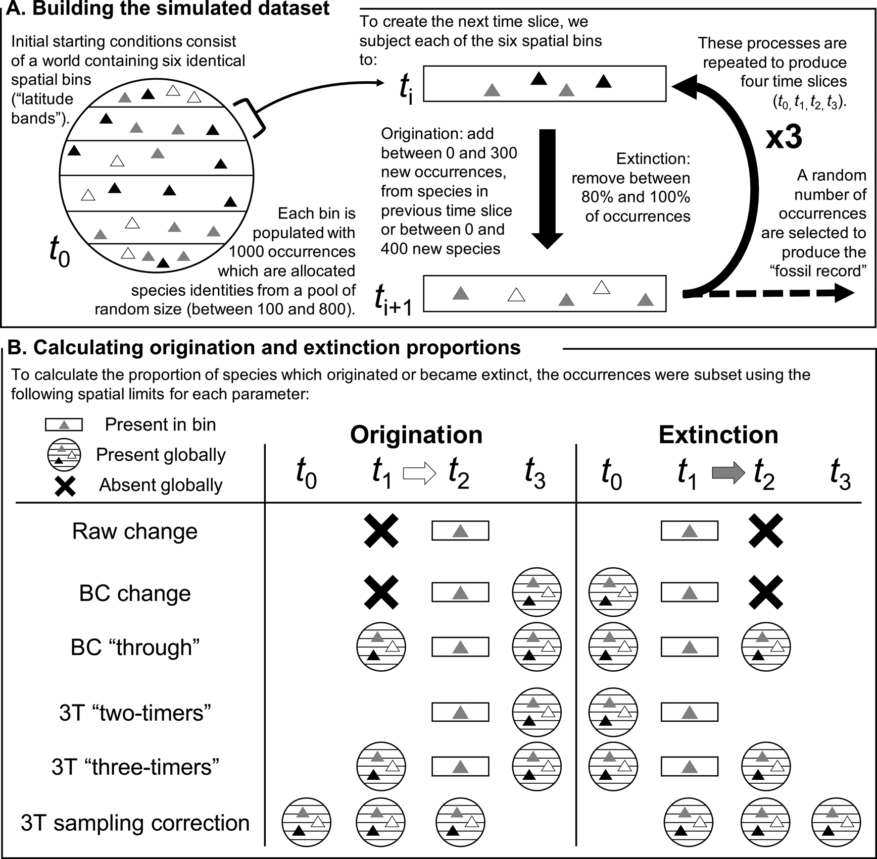
Figure 1. Schematic explaining (A) the construction of the simulated dataset and (B) implementation of the different methods of estimating origination and extinction proportions in a specific spatial bin. The triangles represent occurrences, while their shades indicate the species they belong to. “BC” refers to the “boundary-crosser” method (Foote Reference Foote1999) and “3T” refers to the “three-timer” method (Alroy Reference Alroy2008). The 3T sampling correction is calculated using an equation that evaluates sampling completeness across the global dataset.
Initial starting conditions (t 0) consisted of a “world” split into six spatial bins, each containing 1000 species occurrences (here considered akin to 30° latitudinal bands, but they could equally represent any six spatial subdivisions, such as bioregions, marine basins, or continents; Fig. 1). The size of the global species pool was drawn at random, containing between 100 and 800 species, and each spatial bin was generated independently by drawing species’ identities at random from the global species pool.
The simulated occurrences were then subjected to three iterations of “origination” and “extinction” to produce a four-slice time series (t 0, t 1, t 2, t 3). To produce each subsequent time slice, a random proportion of occurrences from a given spatial bin, between 0% and 20%, were selected to survive, with the others going extinct.
Origination was simulated by adding a random number of occurrences to the spatial bin, between 0 and 300, with their identities selected from a pool consisting of species present in any of the six spatial bins in the previous time slice, plus a random number of new species, selected between 0 and 400. These processes were carried out independently for each spatial bin, operating at the level of a local population. This procedure allowed migration of species between spatial bins across the different time slices: for example, a particular species could suffer local extinction(s) in t 1 but be selected for local origination(s) in t 2, a process that would not be counted as “true” extinction or origination events, regardless of the spatial bins within which these phenomena took place (Fig. 1B). Our simulation design permitted migration between any pair of spatial bins, irrespective of their identities (or apparent positioning relative to one another), in adjacent time slices.
Once each bin had been populated with occurrences, we replicated the sampling filters known to exist in the fossil record by subsampling each spatial bin in every time slice once. The number of occurrences to subsample was drawn from a uniform distribution between 0 and the total number of occurrences, with all occurrences having an equal probability of being selected.
The described simulation protocol was repeated across 10,000 iterations to incorporate variation in origination, extinction, and sampling completeness (Supplementary Fig. S1). We also ran simulations of 5000 iterations using different combinations of low (0 to ~0.2), medium (~0.1–0.3), and high (~0.3–0.5) origination and extinction levels, to investigate the impact of turnover rate on the accuracy of estimates (Supplementary Figs. S6–S11).
Our simulation was purposefully simplistic and therefore may not replicate the complexity of empirical fossil datasets. For example, the six latitudal bins were initially allocated equal numbers of occurrences, which does not reflect the differences in habitat area available across latitudinal bands. Sampling bias was modeled as random, which is an oversimplification of the interaction of the various facets of sampling bias, many of which are at least somewhat systematic (e.g., Darroch et al. Reference Darroch, Casey, Antell, Sweeney and Saupe2020; Benson et al. Reference Benson, Butler, Close, Saupe and Rabosky2021). The ability of species to migrate between any two latitudinal bands is also unrealistic. However, the ways in which species’ ranges shift on geological timescales is poorly understood, and the approach used here avoids applying potentially false assumptions to this facet of the simulation. In this simulation framework, we assumed that common and rare species were equally likely to experience local extinction, but we investigated the impact of this assumption on metric accuracy with further simulations (see “Simulation with Abundance Selectivity”).
Metrics and Their Application
Three metrics designed to estimate global origination and extinction were applied to the simulated data: (1) raw, (2) boundary-crosser (BC) (Alroy Reference Alroy1996; Foote Reference Foote1999), and (3) three-timer (3T) (Alroy Reference Alroy2008). Origination and extinction were calculated as proportions, indicating the fraction of species within the focal time slice, using these metrics (Fig. 1B).
• Raw values were calculated as the proportion of taxa in a given spatial bin that were not represented in the previous (origination) or subsequent (extinction) time interval. Raw values calculated using the complete (unsampled) datasets were deemed the “true” values to which all other estimates were compared.
• The BC method is based on cohort analysis (Raup Reference Raup1978) and evaluates the proportion of taxa that do not cross the “bottom” (originations) or “top” (extinctions) of a given time interval. While the method was developed by Foote (Reference Foote1999), the proportions calculated here are based on the equations of Alroy (Reference Alroy1996), which exclude singletons (species known only from a single time slice).
• The 3T method, described by Alroy (Reference Alroy2008), is also based on cohort analysis, but incorporates an estimate of sampling completeness. The method uses the proportion of “part-timers,” taxa that are present in the first and third slices of a time series but not the second, relative to “three-timers,” which are taxa present in all three time slices, to adjust the calculated proportions of origination and extinction.
The 3T approach has been developed further, including the “gap-filler” (Alroy Reference Alroy2014) and “second-for-third” (Alroy Reference Alroy2015) modifications. These metrics are more complex to calculate, which gives them improved performance when interrogating changes in global biodiversity through time compared with the above three metrics (Alroy Reference Alroy2014, Reference Alroy2015). However, their parameterization makes them difficult to apply to spatially restricted datasets, and thus they are not tested here.
These origination and extinction metrics are usually applied to global datasets, but their application here was altered to estimate origination and extinction within individual spatial bins. The implementation of raw, BC, and 3T methods to assess origination and extinction for a single spatial bin is demonstrated in Figure 1B. Only the focal time slice (t 1 for extinction, t 2 for origination) was filtered to the relevant spatial bin, and all comparisons were made with global datasets in the other time slices. This meant that species that migrated between spatial bins, experiencing local but not global origination and extinction, were not included in estimates. In this approach, sampling bias was particularly important in determining whether species were correctly identified as present within the spatiotemporal bins they occupied, and our subsequent discussion of sampling bias refers to this as the definition of “completeness.” We also calculated metric estimates for each simulation iteration globally, to provide a benchmark for their performance as they are usually applied.
Assessing Metric Performance (without Selectivity)
The performance of the three metrics was assessed using two different approaches. Differencing, that is, subtraction, was used to evaluate the absolute accuracy of estimates for individual spatial bins. Student's t-tests and Cohen's D were used to evaluate whether the distributions of error for each metric had mean values different from 0 and from one another's mean values. The ability to recreate the gradient of origination and extinction proportions across the six spatial bins in a single iteration was also assessed by: (1) evaluating whether the maximum and minimum values were attributed to the same spatial bins; (2) calculating Spearman's rank correlation coefficients between the estimated and “true” values; and (3) quantifying the number of spatial bins with overestimated values, rather than underestimated or identical values, to indicate the consistency of the direction (or sign) of numerical difference within individual iterations or “worlds.”
Simulation with Abundance Selectivity
The first simulation framework assumed no relationship between the number of occurrences of a species and its probability of extinction at a local level. However, this assumption may not be valid in real biological systems (e.g., Brown and Kodric-Brown Reference Brown and Kodric-Brown1977; Fagan et al. Reference Fagan, Unmack, Burgess and Minckley2002; Kiessling and Aberhan Reference Kiessling and Aberhan2007; Hooftman et al. Reference Hooftman, Edwards and Bullock2016; Casey et al. Reference Casey, Saupe and Lieberman2021). We therefore ran additional simulations in which this assumption was relaxed and investigated the possibility of an interaction between sampling completeness and abundance selectivity when estimating evolutionary rates.
To generate the initial dataset, occurrences for each of 400 taxa were drawn from those of Wordian brachiopod genera in the PBDB, to generate a realistic relative abundance distribution. We then simulated an extinction event in this population, with a “true” taxon extinction proportion of around 50%. Extinction selectivity in each trial was determined using a random value from a Poisson distribution, treating zero values as extinction and nonzero values as survival (Fig. 2). Sequences of 400 evenly spaced numbers were generated, with each sequence centered around a value of λ = 0.69 to result in approximately 50% zero and 50% nonzero values. We varied selectivity by altering the range of the sequence around the center, with broader ranges leading to greater differences in extinction risk for rare and common taxa. For example, a sequence of 400 λ values between 1.29 and 0.09 would correspond to extinction risk of 27.5% for the rarest taxon and 91.4% for the commonest taxon. A sequence of 400 λ values between 0.39 and 0.99 would correspond to extinction risk of 67.7% for the rarest taxon and 37.1% for the commonest taxon. A sequence of 400 λ values with a range of 0 (i.e., all λ values are equal to 0.69) would correspond to an extinction risk of approximately 50% for all taxa. We varied the range of the sequences from −1.2 (1.29 to 0.09) to 1.2 (0.09 to 1.29) at increments of 0.002 units, resulting in 1201 different selectivity scenarios.
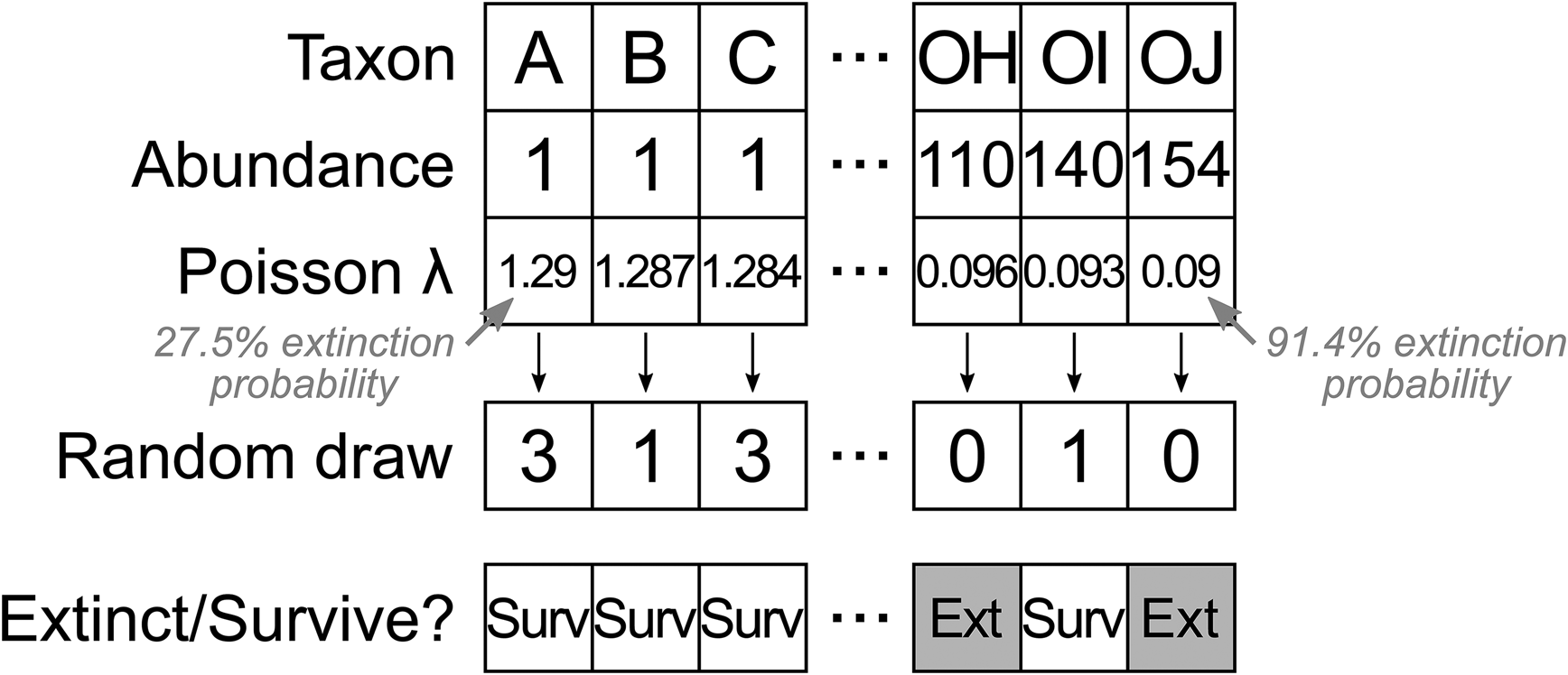
Figure 2. Algorithm for assigning a sequence of λ values to taxa ordered by abundance, converting λ values to a random draw from a Poisson distribution (note that the random draw values represent a single instance and will change in different trials), and discretizing the Poisson counts to extinct (zero value) or survive (nonzero value). This example shows one sequence out of 1201 that resulted in strong selectivity for increased survival of rare taxa.
After assigning survival or extinction status to each taxon, we calculated “true” selectivity using a logistic regression describing the probability of survival as a function of the number of occurrences. The log-odds ratio describes how the odds of survival change for each one-unit increase in a taxon's occurrence count. A positive log-odds ratio corresponds to increased survival among common taxa, and a negative log-odds ratio corresponds to increased survival among rare taxa.
Five different sampling levels were then applied, drawing 10% (“smallest”), 32.5% (“small”), 55% (“medium”), 77.5% (“large”), and 100% (“perfect”) of occurrences. The simulations used all combinations of sampling level and selectivity ranges, resulting in 6005 trials. To evaluate the impact of extinction selectivity based on abundance on the accuracy of extinction estimates, we subtracted the “true” extinction proportion for each simulation from the estimated raw extinction proportion after subsampling.
We also investigated the performance of raw (range through), BC, and 3T extinction metrics under conditions of both varying extinction selectivity and incomplete sampling in specific time bins. We used the same five sampling levels and extinction selectivity method described above, varying sampling in time bin t 0 (the interval immediately preceding the focal time interval) and sampling in time bin t 2 (immediately following the focal time interval). We then examined the combined effects of incomplete sampling in the focal interval t 1, the preceding interval t 0, and the succeeding interval t 2. To keep the number of permutations manageable, for this analysis we used two sampling levels for t 1, 30% (“small”) and 60% (“moderate”) of occurrences, and three sampling levels for t 0 and t 2, 30% (“small”), 60% (“moderate”), and 100% (“perfect”) of occurrences.
Applying Metrics to Permian–Triassic Fossil Data
Having investigated the efficacy of the evolutionary rate estimation metrics, we applied these metrics to the Permian and Triassic marine invertebrate fossil record. Occurrences identified to genus or species level from four major invertebrate clades (Ammonoidea, Bivalvia, Brachiopoda, Gastropoda) were downloaded from the PBDB in March 2021. The occurrences date from the Artinskian (middle early Permian) to the Norian (middle Late Triassic), enabling origination and extinction proportions to be estimated for the Roadian (early middle Permian) to the Ladinian (late Middle Triassic). Uncertain generic identifications were excluded, as were any collections from nonmarine environments or those dated less precisely than to a single stage. The cleaned dataset consisted of a total of 90,209 occurrences.
The paleolatitudes occupied by these fossils were determined by rotating their modern-day locality coordinates back to their time of deposition, stage-by-stage, using the PALEOMAP Global Plate Model (Scotese Reference Scotese2016) implemented in GPlates (Müller et al. Reference Müller, Cannon, Qin, Watson, Gurnis, Williams, Pfaffelmoser, Seton, Russell and Zahirovic2018). Following this, occurrences were allocated to 30° latitudinal bands, approximately representing tropical (0°–30°), temperate (30°–60°), and polar (60°–90°) regions in each hemisphere. Raw, BC, and 3T proportions of origination and extinction were calculated for each latitudinal bin containing more than five genera in every stage, as described in Figure 1B. To increase the completeness of the available fossil record, origination and extinction were evaluated at the genus level, but estimates were also calculated for species (Supplementary Fig. S13).
Results
Metric Performance in Simulation without Selectivity
Individual Spatial Bins
To test the accuracy of the three rate estimation methods when applied regionally, we calculated the numerical difference between estimated proportions of origination and extinction and their corresponding true values for individual spatial bins (n = 6 spatial bins × 10,000 iterations = 60,000 bins). Randomly sampling the simulated occurrences, to emulate the patchy nature of the fossil record, reduced both the precision and accuracy of origination and extinction estimates for all three metrics (Fig. 3, Supplementary Table S1). Following sampling, raw and BC metrics tended to overestimate both origination and extinction (Table 1). The 3T estimates were more accurate, with mean and median differences from the true values much closer to zero, and narrower interquartile ranges (IQRs) (Fig. 3, Table 1). For all metrics, extinction estimates were slightly more accurate than origination estimates. These trends were also seen when applying the metrics to the global datasets (n = 10,000 iterations), but with slightly smaller overall ranges and IQRs (Fig. 3).
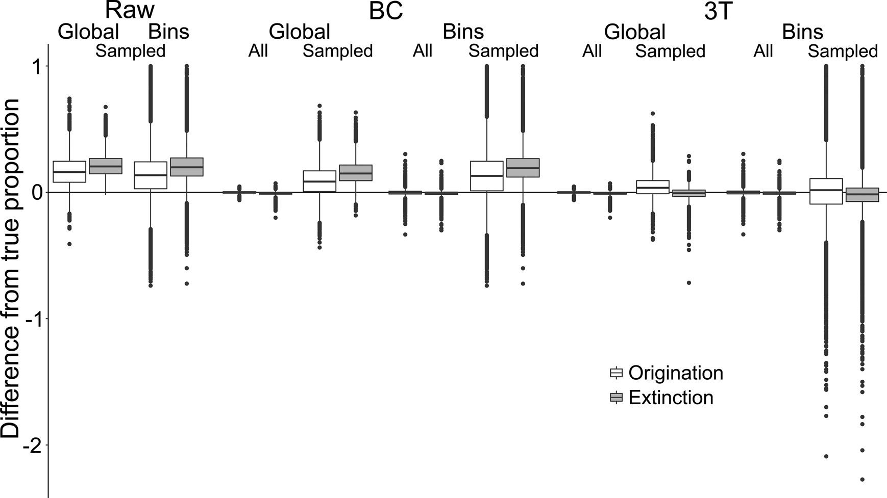
Figure 3. Differences between “true” and estimated proportional origination and extinction. Proportions were compared between global and individual spatial bin scales. “BC” refers to the “boundary-crosser” method (Foote Reference Foote1999) and “3T” refers to the “three-timer” method (Alroy Reference Alroy2008).
Table 1. Results of statistical tests comparing the mean differences between “true” and post-sampling estimated origination and extinction proportions with (A) 0 and (B) each other. Student's t-test was used to determine statistical significance, with p < 0.05 deemed to signify a significant difference. Cohen's D was used to determine effect size, with 0 < D < 0.3 considered a weak effect, 0.3 < D < 0.8 considered a moderate effect, and D > 0.8 considered a strong effect. n (number of samples) was less than the total number of spatial bins tested (6 × 10,000 = 60,000 bins), because some simulations resulted in sample sizes that were too small to allow calculation of the metrics.

Examining estimates based on sampling completeness of the relevant spatial bin revealed that, for all three metrics, the ranges and IQRs of difference reduced as sampling completeness increased (Supplementary Fig. S2b). However, although 3T estimates approached the true values with increased sampling, the raw and BC estimates did not, instead tending toward overestimation of ~0.1–0.2. Additional analyses examining the effect of low versus high origination and extinction levels (0 to ~0.5) on estimate accuracy indicated that the range of differences increased with higher turnover (Supplementary Fig. S8).
Gradient within an Iteration
The accuracy of rate estimation metrics was also assessed by considering the gradient in origination and extinction proportions across spatial bins within a single iteration (n = 10,000 iterations). We compared true and estimated proportions of origination and extinction to test (1) whether maximum and minimum values were attributed to the same spatial bins, (2) whether true and estimated values were correlated with one another, and (3) whether estimated values were consistently overestimated (or underestimated) within each iteration. The gradients of BC and 3T estimates for any given iteration were identical, because the 3T method is effectively the BC method with an added sampling correction that can only be applied at a global level.
After sampling, spatial bins with the highest and lowest proportions of origination and extinction were identified correctly in only a third of the iterations, regardless of the metric used (Supplementary Fig. S3). Raw estimates were slightly more successful than BC and 3T estimates. Across metrics, the spatial bin with the highest proportional origination was identified correctly in more iterations than the bin with the lowest proportional origination. For extinction, bins with the highest and lowest proportional extinction were approximately equally likely to be identified correctly. Additional analyses examining low versus high origination and extinction levels showed that higher turnover resulted in a slight reduction in the ability to correctly identify bins with the lowest and highest proportional origination and extinction (Supplementary Fig. S9).
Rank correlation between post-sampling estimates and true origination and extinction values was assessed using Spearman's ρ (Supplementary Fig. S4). In most iterations, the correlation between post-sampling estimates and true origination and extinction values was positive and of intermediate strength (~0.3–0.7), but with corresponding p-values indicating nonsignificant relationships. These results were also seen in the simulations with low, medium, and high origination and extinction levels (Supplementary Fig. S10).
The proportion of spatial bins within each iteration that overestimated proportional origination and extinction (Supplementary Fig. S5) had a similar distribution to that of individual spatial bins (Fig. 2). Following sampling, raw and BC estimates generally overestimated proportional origination and extinction in five, or all six, of the spatial bins. In contrast, 3T estimates tended to overestimate proportional origination and extinction in two to four of the six spatial bins, suggesting a relatively even distribution of differences above and below the true values within a single iteration.
Metric Performance in Simulation with Abundance Selectivity
Our simulations indicated that estimated extinction proportions were increasingly biased as the strength of the relationship between abundance and extinction increased and as sampling completeness decreased (Fig. 4). If common taxa were more likely to survive, as is often assumed to be the case, smaller subsamples resulted in a lower extinction estimate. This bias exists because a smaller subsample is less likely to capture rare taxa, and common taxa will be relatively overrepresented, leading to lower estimated extinction levels in the subsample. Conversely, if rare taxa are more likely to survive, smaller subsamples will tend to overestimate extinction.
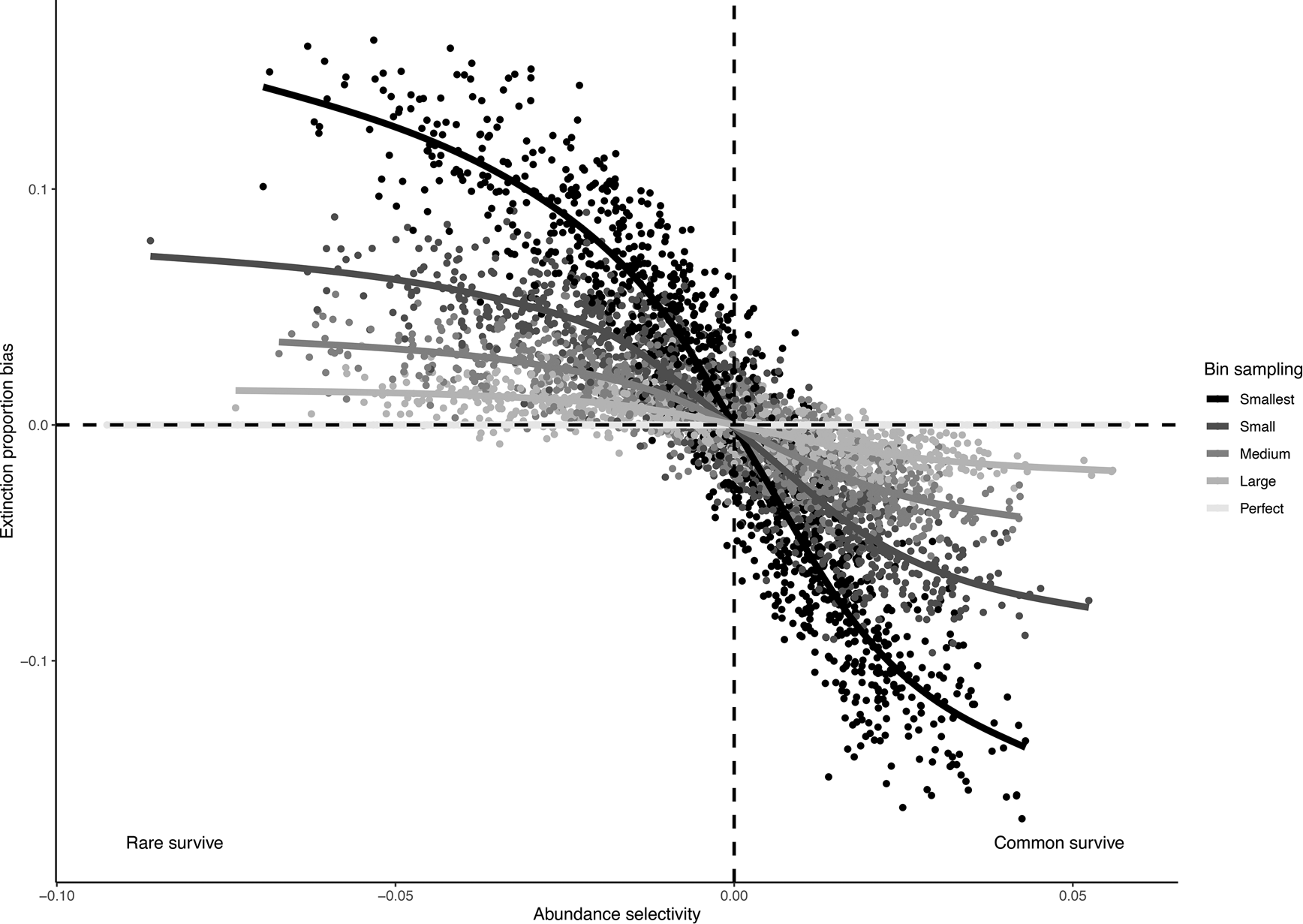
Figure 4. Bias in observed extinction proportions under different simulation conditions of selectivity and subsample size. Positive bias indicates an overestimation relative to the “true” extinction rate; negative bias indicates an underestimation of extinction. Selectivity is measured by the log-odds ratio for the effect of abundance on survival, and sample size of the five different data subsets is indicated using different shades.
Incomplete sampling of the t 0 interval produced a similar bias in the BC and 3T methods and had the same outcome as incomplete sampling of the focal interval t 1 (Fig. 5, Supplementary Fig. S12). This is because removing a taxon from t 0 meant that it was no longer a boundary-crosser or “two-timer,” and was therefore not counted in the extinction estimate calculation. Rare taxa are preferentially removed as sampling becomes poorer, resulting in a relative overrepresentation of common taxa in the BC cohort in t 1 (the focal interval). The range through method was unaffected when the t 0 bin was undersampled, because this method calculates extinction using data from only the t 1 and t 2 bins.
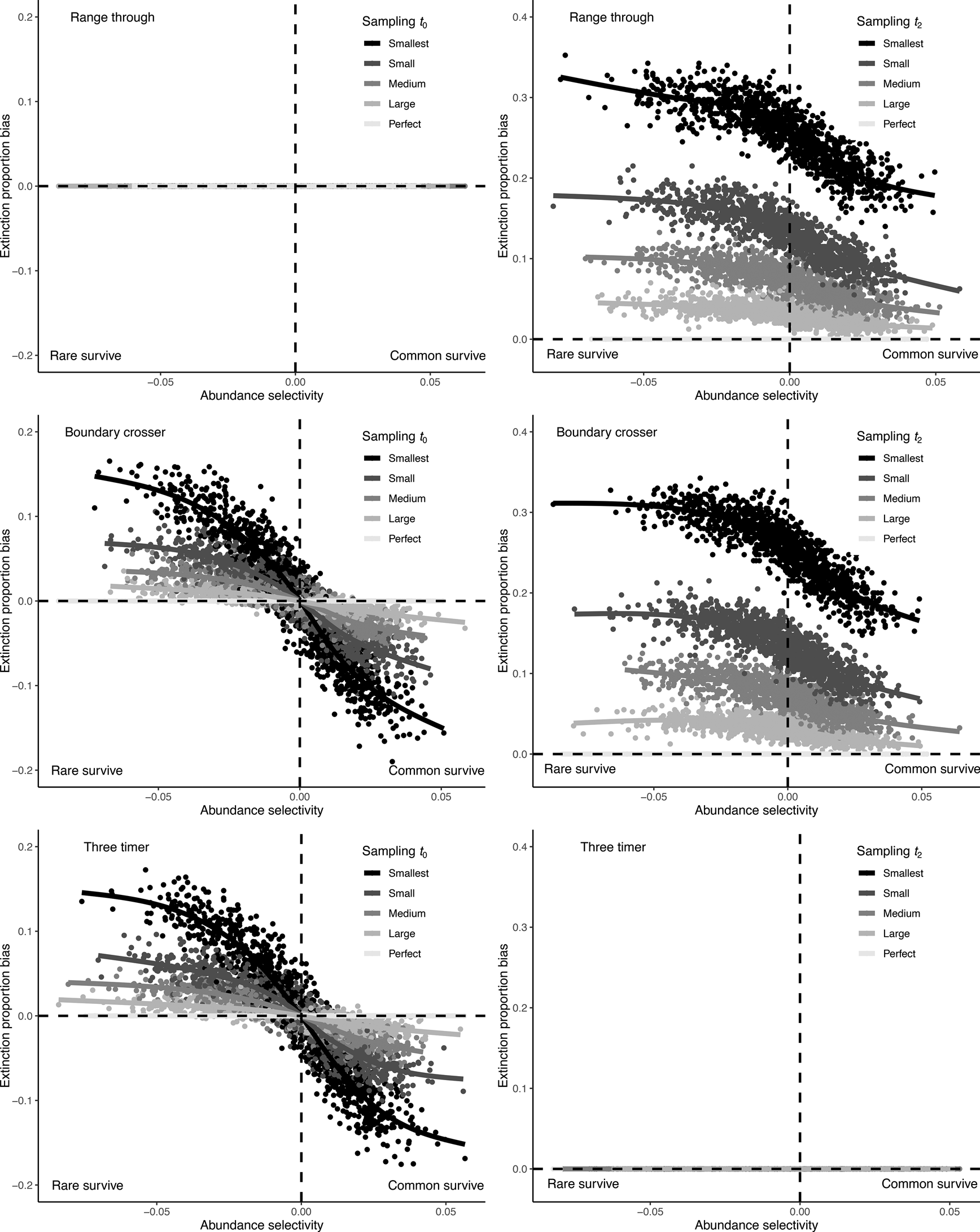
Figure 5. Bias in observed extinction proportions under different simulation conditions of selectivity and subsample size, comparing range through, boundary-crosser, and three-timer extinction rates when the preceding t 0 bin or succeeding t 2 bin are incompletely sampled.
Incomplete sampling of the t 2 interval had the largest effect on extinction estimate bias for the BC method and also strongly affected the accuracy of the range through method (Fig. 5, Supplementary Fig. S12). This occurs because failure to sample a taxon in t 2 means it will be erroneously marked as extinct in t 1, rather than marked as surviving. The extent of the bias also differed as a function of selectivity; if rare taxa were more likely to survive the extinction, they were also more likely to be missed when t 2 was incompletely sampled, inflating extinction estimates. The 3T extinction metric was unaffected by incomplete sampling of t 2 in this simulation, because the calculation is designed to use part-timer taxa (those present in t 1 and t 3, but missing from t 2) to correct for sampling incompleteness in t 2.
None of the three methods tested here are immune from bias due to abundance selectivity. However, the 3T method was generally less biased than the raw (range through) and BC methods, unless the t 2 interval was perfectly sampled. When the t 0 interval was poorly sampled but t 2 sampling was perfect, the range through method performed best.
Regional Evolutionary Rate Estimates for Permian–Triassic Marine Invertebrates
The marine invertebrate fossil record for the Permian and Triassic varies considerably in sampling completeness across space, through time, and among clades (Supplementary Tables S2, S3). As a result, origination and extinction metrics could not be calculated for some of the spatiotemporal (latitude by stage) bins, particularly using the BC and 3T metrics, which have a higher sample size threshold (Fig. 6). Species-level analyses produced similar trends to those at the generic level but with generally higher levels of origination and extinction (Supplementary Fig. S13).
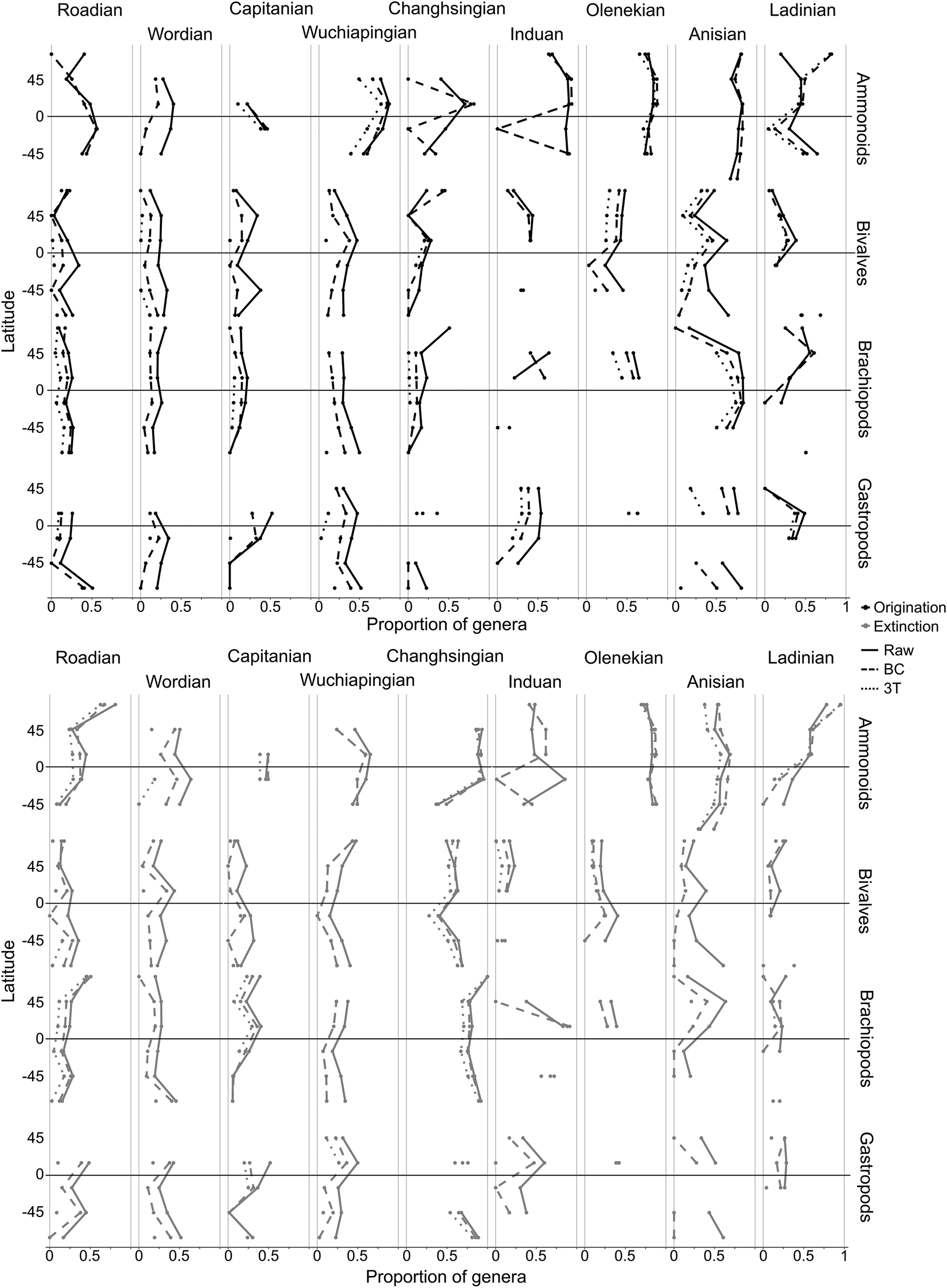
Figure 6. Estimated generic-level origination and extinction by latitude for four different marine clades in each stage of the middle Permian to Middle Triassic. Occurrences were split into six 30° latitude bins. Estimates were calculated for each spatiotemporal bin containing five or more genera. Missing points indicate insufficient occurrences to calculate a proportion. “BC” refers to the “boundary-crosser” method (Foote Reference Foote1999) and “3T” refers to the “three-timer” method (Alroy Reference Alroy2008).
Origination and extinction appear to have been uniformly low across latitudes for marine invertebrates in the Permian, predominately below 50% of genera (Fig. 6). There is little evidence of heightened extinction in the Capitanian, although ammonoids underwent considerable diversification in the Wuchiapingian, particularly at low latitudes (around 80% of genera).
The effect of the PTME is clearly visible, with high extinction globally in the Changhsingian. Ammonoids experienced highest extinction levels at low latitudes (around 90%) and reduced extinction in the southern midlatitudes (around 40%). Brachiopods and bivalves appear to have exhibited the opposite gradient, with slightly lower extinction proportions at low latitudes (around 70% at low latitudes vs. 90% at high latitudes for brachiopods, and 40% at low latitudes vs. 65% at high latitudes for bivalves).
The brachiopod, bivalve, and gastropod records are sparse during the Early Triassic, particularly in the Southern Hemisphere, hindering reliable rate estimation. Origination appears not to have been unusually high in the Induan, in the aftermath of the mass extinction, except perhaps for the ammonoids (around 85%). Although extinction was generally reduced and spatially uniform in the Induan, brachiopods experienced a high proportion of extinction in the low northern latitudes. Ammonoids underwent both high origination and extinction globally in the Olenekian (both around 85%), indicating rapid turnover in the clade, whereas bivalves experienced reduced extinction rates (around 20%). In the Middle Triassic, origination and extinction gradients became more spatially uniform and stable for all four clades, although ammonoids appear to have undergone turnover in the high northern latitudes during the Ladinian.
Discussion
Regional Rate Simulation Performance
Our results indicate that in the absence of abundance-based extinction selectivity, raw, BC, and 3T origination and extinction metrics can be applied to spatially subdivided datasets of fossil occurrences, producing estimates with only slightly less accuracy than when used globally (Fig. 3, Supplementary Fig. S2). This inaccuracy is likely partly due to the reduction in sample size (number of occurrences) resulting from creating spatial subdivisions within a global dataset. However, sampling incompleteness reduces the accuracy of origination and extinction rate estimation considerably (Supplementary Fig. S2b), as does the potential presence of extinction selectivity based on taxon abundance (Fig. 5).
The 3T estimates were generally more accurate than those calculated using raw or BC methods (Figs. 3, 5, Supplementary Fig. S2, Table 1). However, the 3T method requires occurrences to be present across multiple time slices (Fig. 1), a condition that may not always be met. BC estimates produced the same gradient of origination and extinction in latitude bins within a given iteration, and so can be used as a reasonable compromise when comparing estimates within a time slice. Raw estimates were slightly more successful at identifying spatial bins with the highest and lowest levels of origination and extinction (Supplementary Fig. S3). As a result, choice of metric should depend on the analysis required; we recommend calculating more than one metric, when possible, to allow for comparison.
The most accurate estimates were produced using the 3T method on spatial bins with a high sampling completeness (Fig. 5, Supplementary Fig. S2b), and variation in sampling completeness between spatial bins appears to hinder efforts to identify the bins that experienced highest and lowest origination and extinction (Supplementary Figs. S3, S9). Using higher taxonomic levels may increase the number of usable occurrences, but the patterns observed should not be assumed to be analogous to trends at lower taxonomic levels (Hendricks et al. Reference Hendricks, Saupe, Myers, Hermsen and Allmon2014).
Estimates produced for low levels of origination and extinction were slightly more accurate than those for high levels of origination and extinction (Supplementary Fig. S8). This was expected for BC and 3T estimates; these methods exclude singletons, so when turnover rates increase, a larger proportion of species are represented as singletons in the fossil record, and the effective sample size is reduced. However, the difference in accuracy observed in the simulated data is relatively small, and therefore the uncertainty around high origination and extinction estimates should not be considered greater than that around smaller estimates.
Additional investigation using more complex simulations might reveal how the three rate metrics used here could be modified to produce more accurate results in a regional context, or whether a correction could be used to account for any regular overestimation in rate estimates (Supplementary Fig. S2b). Potential also exists for the development of metrics specific to estimating spatial variation in rates, including adaptation of the gap-filler and second-for-third methods, which perform better than raw, BC and 3T metrics when applied to global datasets (Alroy Reference Alroy2014, Reference Alroy2015). The resilience of these metrics to abundance-based extinction selectivity will also need to be tested. Simulation approaches might also hold potential for investigating how best to estimate migration rates from the fossil record.
Permian–Triassic Origination and Extinction across Latitudes
Analyses of Permian–Triassic marine invertebrates provide little evidence for high extinction in any of the studied clades during the CBC (Fig. 6). Brachiopods experienced slightly higher extinction in the low and high northern latitudes (around 40% of genera), which supports the results of Clapham (Reference Clapham2015), who identified a generic turnover in Capitanian–Wuchiapingian faunas from Iran and South China. Extinction in the clade was higher at the species level, particularly in the Northern Hemisphere (around 75%; Supplementary Fig. S13), which is somewhat lower than the 87% reported by Shen and Shi (Reference Shen and Shi1996) for South China.
Globally, low origination and extinction levels (both around 20%) indicate that bivalves appear to have been largely unaffected by the CBC, in agreement with Bond et al. (Reference Bond, Hilton, Wignall, Ali, Stevens, Sun and Lai2010). By contrast, ammonoids and gastropods experienced moderate extinction levels at low latitudes (around 50%) during the CBC. Our results support a generic turnover of ammonoids during the Capitanian (Villier and Korn Reference Villier and Korn2004; Rampino and Shen Reference Rampino and Shen2019), but the clade's fossil record is highly spatially restricted at this time, so it is unclear whether this turnover took place globally or only in the southern low latitudes. We found high ammonoid origination levels across low to midlatitudes in the Wuchiapingian, in agreement with Clapham et al. (Reference Clapham, Shen and Bottjer2009) and McGhee et al. (Reference McGhee, Clapham, Sheehan, Bottjer and Droser2013). Collectively, the results presented here support the hypothesis that the CBC was highly selective (McGhee et al. Reference McGhee, Clapham, Sheehan, Bottjer and Droser2013), with some marine clades undergoing turnover, particularly at low latitudes (ammonoids and gastropods), while others were seemingly unaffected (bivalves and brachiopods).
High extinction levels during the Changhsingian, which mark the PTME, are seen globally in all four marine invertebrate clades. For bivalves, gastropods, and brachiopods, the highest extinction levels were observed at mid- to high latitudes. These results support those of Reddin et al. (Reference Reddin, Kocsis and Kiessling2019), who reported that benthic marine invertebrates experienced higher extinction rates away from the equator during the PTME. However, slightly reduced extinction levels at low latitudes in these clades may be an artifact caused by the occurrence of “mixed faunas.” These are communities of benthic invertebrates, particularly well known from sections in low-latitude South China, that survived the Changhsingian only to become extinct in the earliest Induan (Song et al. Reference Song, Wignall, Tong and Yin2013). The presence of a low-latitude Induan extinction peak for brachiopods marks the loss of these mixed faunas. In contrast, ammonoids experienced the highest Changhsingian extinction levels at low latitudes. The late Permian ammonoid fossil record is relatively spatially restricted in comparison with the Early Triassic record, which may contribute to this result (Dai and Song Reference Dai and Song2020); that is, low extinction in the southern midlatitudes corresponds to a handful of localities in northern India and may therefore reflect relatively incomplete sampling.
Bivalves, gastropods, and ammonoids appear to have experienced highest origination at low latitudes during the Induan. The discrepancy between raw and BC rates for some ammonoid and brachiopod latitudinal bins during this interval is likely due to “disaster faunas,” which contributed a high number of temporal singletons. Ammonoids underwent rapid turnover across latitudes in the Olenekian, which coincides with an observed increase in their endemism during this time, and the influence of a possible extinction event around the Smithian/Spathian boundary (~250 Ma) (Brayard et al. Reference Brayard, Bucher, Escarguel, Fluteau, Bourquin and Galfetti2006; Song et al. Reference Song, Wignall, Chen, Tong, Bond, Lai, Zhao, Jiang, Yan, Niu, Chen, Yang and Wang2011; Wignall Reference Wignall2015; Dai and Song Reference Dai and Song2020). For all four clades, origination and extinction reduced and became more globally homogenous in the Anisian and Ladinian, corresponding to the amelioration of global temperatures and the re-establishment of diverse benthic communities (Sun et al. Reference Sun, Joachimski, Wignall, Yan, Chen, Jiang, Wang and Lai2012; Martindale et al. Reference Martindale, Foster and Velledits2019).
In summary, both origination and extinction were relatively consistent across latitudes for all four clades throughout the middle Permian to Middle Triassic (Fig. 6). Minor variation in rates was observed through time and between latitudinal bins, but caution should be exercised in interpreting any observed differences as indicative of contrasting evolutionary dynamics across latitudes rather than reflecting noise or sampling bias. The taxonomic identity of a genus appears to be a more important factor in determining extinction vulnerability than the paleolatitudes occupied, indicating a stronger phylogenetic signal in selectivity than that for latitude.
Although the scale of estimated variation between latitudinal bands is limited, the Changhsingian latitudinal gradients of extinction seen in benthic clades (bivalves, brachiopods, gastropods) align with the hypothesis that extinction during the PTME was most severe at high latitudes due to loss of suitable habitat for cool-adapted taxa, as advocated for by Penn et al. (Reference Penn, Deutsch, Payne and Sperling2018). By contrast, the extinction gradient of ammonoids, the only pelagic clade examined here, better fits the hypothesis that extremely high equatorial temperatures resulted in tropical extinction and poleward migration, a mechanism proposed by Sun et al. (Reference Sun, Joachimski, Wignall, Yan, Chen, Jiang, Wang and Lai2012) and supported by Song et al. (Reference Song, Huang, Jia, Dai, Wignall and Dunhill2020) and Flannery-Sutherland et al. (Reference Flannery-Sutherland, Silvestro and Benton2022). Our results therefore suggest a possible contrast in spatial patterns of PTME extinction based on paleoecology. Variation in the rate of post-PTME recovery has previously been identified between these two ecologies, with ammonoids and conodonts recovering more rapidly than benthic animals (Brayard et al. Reference Brayard, Bucher, Escarguel, Fluteau, Bourquin and Galfetti2006; Song et al. Reference Song, Wignall, Chen, Tong, Bond, Lai, Zhao, Jiang, Yan, Niu, Chen, Yang and Wang2011, Reference Song, Wignall and Dunhill2018; Martindale et al. Reference Martindale, Foster and Velledits2019), a trend also observed after the Triassic–Jurassic mass extinction (Dunhill et al. Reference Dunhill, Foster, Azaele, Sciberras and Twitchett2018). Penn et al. (Reference Penn, Deutsch, Payne and Sperling2018) hypothesized that these two contrasting extinction gradients may reflect differences in primary kill mechanism, with extinctions at higher latitudes linked to oxygen depletion, and extinctions at low latitudes linked to temperatures beyond thermal tolerance levels. Oceanic oxygen depletion tends to be more severe in bottom waters (e.g., Liao et al. Reference Liao, Wang, Kershaw, Weng and Yang2010), leaving benthic animals more vulnerable to anoxia than pelagic animals. In addition, the elevated extinction levels experienced by ammonoids during the late Smithian thermal maximum may support a higher sensitivity to extremes of temperature within the clade (Dai and Song Reference Dai and Song2020).
Although it is tempting to accept the above narrative, the results derive from an incomplete and biased fossil record, imperfect rate estimation metrics, and small differences between rate estimates across time and latitudes. Extinction selectivity based on abundance may have also reduced the accuracy of our estimates. As such, we advocate for additional assessment of latitudinal variation in Permian–Triassic evolutionary rates in the future, with larger datasets and more robust metrics, ideally designed specifically to estimate variation in evolutionary rates across space. Investigating spatial variation in origination and extinction in other pelagic clades, such as conodonts and fishes, and directly testing the timing and direction of migration in marine invertebrates, may also provide further insight into the nature of biotic responses to the PTME in the marine realm.
Conclusions
Using simulations, we demonstrate that it is possible to estimate origination and extinction patterns across space from the fossil record with reasonable accuracy, albeit under conditions of relatively complete sampling and no extinction selectivity based on taxon abundance. We applied rate estimation metrics to marine invertebrates from the Permian and Triassic to test previously posited hypotheses on the latitudes at which the highest extinction rates occurred during the PTME. Both origination and extinction were found to be generally uniform across latitudes throughout the study interval. Larger fossil datasets with better geographic spread and more robust metrics would be necessary to confirm whether any deviations in origination and extinction are not simply a result of sampling bias, and of a sufficient magnitude to be deemed evolutionarily important. Our results indicate that origination and extinction levels during the PTME were more dependent on taxonomic identity than latitudinal occupation.
Acknowledgments
We thank members of the Palaeo@Leeds, Ecosystem Resilience and Recovery from the Permo-Triassic Crisis (Eco-PT), and Computational Evolution (cEvo) research groups for discussion, and P. Mannion and T. Aze for their constructive criticism of earlier versions of this article. We are grateful to M. Powell and an anonymous reviewer, whose comments greatly improved this article. We thank all those who have contributed toward the Paleobiology Database collections used in this study. This is Paleobiology Database publication no. 440. B.J.A. commenced this work during her Ph.D. at the University of Leeds, funded by a U.K. Natural Environment Research Council studentship (NE/L002574/1) and has since been supported by an ETH+ grant (BECCY) funded by ETH Zurich. P.B.W and A.M.D. were both supported by the Eco-PT grant (NE/P0137224/1), part of the Biosphere Evolutionary Transitions and Resilience (BETR) project, jointly funded by the U.K. Natural Environment Research Council and National Natural Science Foundation of China. E.E.S. was supported by a Leverhulme Prize and Leverhulme grant (DGR01020) and NERC grant (NE/V011405/1).
Declaration of Competing Interests
The authors declare no competing interests.
Data Availability Statement
Data available from the Zenodo Digital Repository: https://doi.org/10.5281/zenodo.7355273.


 Open access