


1 Introduction
Birational classification of complex algebraic varieties is a central research area in algebraic geometry. Given an algebraic variety, one can produce a somewhat simpler birational model of it by first taking a resolution of singularities and then running the minimal model program (MMP). We work in dimension $3$
and over the field of complex numbers, where both these theories are settled. The result of this procedure is either a Mori fiber space or a minimal model, depending on whether the initial variety was uniruled or not. We are interested in explicit classification of Mori fiber spaces, that is, the study or birational relations among Mori fiber spaces as end points of the MMP. A Mori fiber space can be a unique product of the MMP, so-called Birationally Rigid, and can have a few, or infinitely many birational models (see Definition 1.2 for a precise definition of rigidity). For example, a smooth quartic in
$3$
and over the field of complex numbers, where both these theories are settled. The result of this procedure is either a Mori fiber space or a minimal model, depending on whether the initial variety was uniruled or not. We are interested in explicit classification of Mori fiber spaces, that is, the study or birational relations among Mori fiber spaces as end points of the MMP. A Mori fiber space can be a unique product of the MMP, so-called Birationally Rigid, and can have a few, or infinitely many birational models (see Definition 1.2 for a precise definition of rigidity). For example, a smooth quartic in $\mathbb {P}^4$
is known to be birationally rigid [Reference Iskovskih and Manin18], whereas a quartic with a single
$\mathbb {P}^4$
is known to be birationally rigid [Reference Iskovskih and Manin18], whereas a quartic with a single $cA_2$
singular point has precisely two birational models [Reference Corti and Mella12]. On the other hand, the projective space
$cA_2$
singular point has precisely two birational models [Reference Corti and Mella12]. On the other hand, the projective space $\mathbb {P}^3$
is birational to any Fano variety
$\mathbb {P}^3$
is birational to any Fano variety $V_{22}$
, whose moduli contain an uncountable set (see, e.g., [Reference Kuznetsov and Prokhorov23]).
$V_{22}$
, whose moduli contain an uncountable set (see, e.g., [Reference Kuznetsov and Prokhorov23]).
A Mori fiber space is a normal projective variety X together with a morphism $\pi \colon X\rightarrow S$
with connected fibers to a lower-dimensional variety S, where
$\pi \colon X\rightarrow S$
with connected fibers to a lower-dimensional variety S, where
-
• X is $\mathbb {Q}$
-factorial with terminal singularities,
$\mathbb {Q}$
-factorial with terminal singularities, -
•
$-K_X$
is
$\pi $
-ample, and -
• the relative Picard number
$\rho _{X/S}$
is
$1$
.


Based on the dimension of S, either X is a conic bundle over the surface S, or it is a fibration of del Pezzo surfaces over a curve S, or it is a Fano threefold when S is a point.
Definition 1.1. Let $\pi _X \colon X \to S$
and
$\pi _X \colon X \to S$
and $\pi _Y \colon Y \to Z$
be Mori fiber spaces. A birational map
$\chi \colon X \dashrightarrow Y$
$\pi _Y \colon Y \to Z$
be Mori fiber spaces. A birational map
$\chi \colon X \dashrightarrow Y$
 is called square if it fits into a commutative diagram

where g is birational and, in addition, the induced map on the generic fibers
$\chi _\eta \colon X_\eta \dashrightarrow Y_\eta $
 is an isomorphism. In this case, we say that $X/S$
and
$X/S$
and $Y/Z$
are square-birational.
$Y/Z$
are square-birational.
Definition 1.2 [Reference Corti11, Def. 1.2].
A Mori fiber space $\pi _X\colon X\rightarrow S$
is said to be birationally rigid if existence of a birational map
$\pi _X\colon X\rightarrow S$
is said to be birationally rigid if existence of a birational map $\chi \colon X\dashrightarrow Y$
to a Mori fiber space
$\chi \colon X\dashrightarrow Y$
to a Mori fiber space $\pi _Y\colon Y\to Z$
implies that there exists a birational self-map
$\pi _Y\colon Y\to Z$
implies that there exists a birational self-map $\varphi \colon X\dashrightarrow X$
such that the birational map
$\varphi \colon X\dashrightarrow X$
such that the birational map $\chi \circ \varphi $
is square.
$\chi \circ \varphi $
is square.
Birational rigidity of conic bundles has been studied extensively (see, e.g., [Reference Sarkisov31]). The reader is encouraged to consult [Reference Corti11, §4] for an overview and some interesting related questions on birational geometry of conic bundles. Comparatively, the question of (stable) nonrationality of conic bundles has recently had more development [Reference Ahmadinezhad and Okada4], [Reference Böhning and von Bothmer8], [Reference Hassett, Kresch and Tschinkel16]. Birational rigidity and nonrationality of Fano threefolds has progressed in the past decades, but is yet to be completed (see [Reference Hassett and Tschinkel17], [Reference Okada25] for rationality and [Reference Ahmadinezhad and Okada6] for birational rigidity and investigate the references therein for further details). The focus of this paper is on birational rigidity of threefold del Pezzo fibrations.
del Pezzo fibrations form 10 classes, according to their degrees $1\leq d\leq 9$
, and there are two classes in degree 8. If the degree is
$1\leq d\leq 9$
, and there are two classes in degree 8. If the degree is $5$
or higher, then the fibration is rational over the base [Reference Colliot-Thélène10], [Reference Manin24]. Degree
$5$
or higher, then the fibration is rational over the base [Reference Colliot-Thélène10], [Reference Manin24]. Degree $4$
fibrations admit a conic bundle structure [Reference Alekseev7], and hence they are not birationally rigid. Their stable rationality was recently studied in [Reference Hassett and Tschinkel17].
$4$
fibrations admit a conic bundle structure [Reference Alekseev7], and hence they are not birationally rigid. Their stable rationality was recently studied in [Reference Hassett and Tschinkel17].
A smooth degree $2$
del Pezzo surface can be defined as the zeros of a quartic form in
$2$
del Pezzo surface can be defined as the zeros of a quartic form in $\mathbb {P}(1,1,1,2)$
, and a general such form defines a smooth del Pezzo surface of degree
$\mathbb {P}(1,1,1,2)$
, and a general such form defines a smooth del Pezzo surface of degree $2$
. However, when defined over a base curve, this typically has some orbifold singularities of type
$2$
. However, when defined over a base curve, this typically has some orbifold singularities of type $\frac {1}{2}(1,1,1)$
enforced by the zeros of the coefficient of the quadratic monomial in the defining polynomial of the threefold (see [Reference Reid30, §1] for notation and explanation of this type of singularities). This coefficient degree imposes a discrete invariant that splits the moduli space of such fibrations into an infinite set of families. As a result, whenever we use the term general, we mean general after fixing a family. In low degrees, most results on birational rigidity concentrate on smooth models, for example, stable rationality of very general del Pezzo fibrations in low degrees with smooth total space was recently studied in [Reference Krylov and Okada22]. Smoothness of the total space is a strong restriction in degrees
$\frac {1}{2}(1,1,1)$
enforced by the zeros of the coefficient of the quadratic monomial in the defining polynomial of the threefold (see [Reference Reid30, §1] for notation and explanation of this type of singularities). This coefficient degree imposes a discrete invariant that splits the moduli space of such fibrations into an infinite set of families. As a result, whenever we use the term general, we mean general after fixing a family. In low degrees, most results on birational rigidity concentrate on smooth models, for example, stable rationality of very general del Pezzo fibrations in low degrees with smooth total space was recently studied in [Reference Krylov and Okada22]. Smoothness of the total space is a strong restriction in degrees $1$
and
$1$
and $2$
as they are satisfied in very few families. However, a general cubic surface (degree
$2$
as they are satisfied in very few families. However, a general cubic surface (degree $3$
del Pezzo) fibration has smooth total space, which is no longer true in degrees
$3$
del Pezzo) fibration has smooth total space, which is no longer true in degrees $1$
and
$1$
and $2$
.
$2$
.
The following is the main result in the literature for birational rigidity of del Pezzo fibrations over $\mathbb {P}^1$
with smooth total space, which was later improved slightly by Grinenko [Reference Grinenko13]–[Reference Grinenko15] and Sobolev [Reference Sobolev33], also with the smoothness condition.
$\mathbb {P}^1$
with smooth total space, which was later improved slightly by Grinenko [Reference Grinenko13]–[Reference Grinenko15] and Sobolev [Reference Sobolev33], also with the smoothness condition.
Theorem 1.3 [Reference Pukhlikov28, Th. 2.1].
Let $\pi :X \to \mathbb {P}^1$
be a del Pezzo fibration of degree
$\pi :X \to \mathbb {P}^1$
be a del Pezzo fibration of degree $1$
,
$1$
, $2$
, or
$2$
, or $3$
, with smooth X, and assume generality in degree
$3$
, with smooth X, and assume generality in degree $3$
. If
$3$
. If $K_X^2$
is not in the interior of the Mori cone of effective
$K_X^2$
is not in the interior of the Mori cone of effective $1$
-cycles
$1$
-cycles $\overline {\operatorname {NE}}(X)^o$
, then X is birationally rigid.
$\overline {\operatorname {NE}}(X)^o$
, then X is birationally rigid.
This theorem is the center of attention in this article. The only birational rigidity statement for del Pezzo fibrations of low degree with quotient singularities is proved in [Reference Krylov21], which proves Pukhlikov’s theorem above for special families of fibrations with such singularities. We generalize these results for the general case with orbifold families of del Pezzo fibrations in degree $2$
in the following precise setting. There is a fundamental difference in the geometry of the models in the general case, which makes the proof more complicated: the singular points produce elementary Sarkisov links to other models square-birational to X, and that the construction of the staircase (explained below) for smooth points near the singular point is more complex.
$2$
in the following precise setting. There is a fundamental difference in the geometry of the models in the general case, which makes the proof more complicated: the singular points produce elementary Sarkisov links to other models square-birational to X, and that the construction of the staircase (explained below) for smooth points near the singular point is more complex.
Main Theorem. Let $\pi \colon X \to \mathbb {P}^1$
be a del Pezzo fibration of degree
$\pi \colon X \to \mathbb {P}^1$
be a del Pezzo fibration of degree $2$
. Suppose X is a general quasi-smooth hypersurface in a
$2$
. Suppose X is a general quasi-smooth hypersurface in a $\mathbb {P}(1,1,1,2)$
-bundle over
$\mathbb {P}(1,1,1,2)$
-bundle over $\mathbb {P}^1$
satisfying the
$\mathbb {P}^1$
satisfying the $K^2$
-total condition. Then X is birationally rigid.
$K^2$
-total condition. Then X is birationally rigid.
1.1 Conditions in the Main Theorem
Here, we spell out assumptions in the theorem above, and explain their necessity.
1.1.1 Quasi-smoothness
Quasi-smooth means that no singularities come from the defining equation of X, and hence all singularities are indeed of type $\frac {1}{2}(1,1,1)$
and inherited from the ambient toric variety (see Remark 1.5 for a precise definition). This condition cannot be removed as there exists an example of a nonbirationally rigid degree 2 del Pezzo fibration satisfying other conditions that has a nontoric singular point [Reference Ahmadinezhad2].
$\frac {1}{2}(1,1,1)$
and inherited from the ambient toric variety (see Remark 1.5 for a precise definition). This condition cannot be removed as there exists an example of a nonbirationally rigid degree 2 del Pezzo fibration satisfying other conditions that has a nontoric singular point [Reference Ahmadinezhad2].
1.1.2 The
$K^2$
-total condition

The $K^2$
-condition is precisely as in Theorem 1.3, that is,
$K^2$
-condition is precisely as in Theorem 1.3, that is, $K_X^2\notin \overline {\operatorname {NE}}(X)^o$
. For every singular point Q of X, there is a Sarkisov link starting by blowing up X at Q and resulting in a new quasi-smooth model of X, that is, square-birational. This manoeuvre is explicitly described in §4. Let N be the number of singularities of X and denote the singular points by
$K_X^2\notin \overline {\operatorname {NE}}(X)^o$
. For every singular point Q of X, there is a Sarkisov link starting by blowing up X at Q and resulting in a new quasi-smooth model of X, that is, square-birational. This manoeuvre is explicitly described in §4. Let N be the number of singularities of X and denote the singular points by $Q_i$
for
$Q_i$
for $i \in \{1,\dots ,N \}$
. Denoting by
$i \in \{1,\dots ,N \}$
. Denoting by $X_I$
the model acquired by combining the elementary links corresponding to
$X_I$
the model acquired by combining the elementary links corresponding to $Q_i$
,
$Q_i$
, $i \in I$
,
$i \in I$
, $I\subset \{1,\dots ,N \}$
, we say X satisfies the
$I\subset \{1,\dots ,N \}$
, we say X satisfies the $K^2$
-total condition if for every
$K^2$
-total condition if for every $I \subset \{1,\dots ,N\}$
the model
$I \subset \{1,\dots ,N\}$
the model $X_I$
satisfies the
$X_I$
satisfies the $K^2$
-condition. We are convinced that
$K^2$
-condition. We are convinced that $K^2$
-condition on X may be enough, and the totality assumption is redundant. In §4, we give an explicit recipe for constructing all
$K^2$
-condition on X may be enough, and the totality assumption is redundant. In §4, we give an explicit recipe for constructing all $X_I$
models from X. Given X embedded in a
$X_I$
models from X. Given X embedded in a $\mathbb {P}(1,1,1,2)$
-bundle, it is rather easy to check this condition using the recipe. Note that in [Reference Shokurov and Choi32, Cor. 6.4], it is stated that X is birationally rigid if the
$\mathbb {P}(1,1,1,2)$
-bundle, it is rather easy to check this condition using the recipe. Note that in [Reference Shokurov and Choi32, Cor. 6.4], it is stated that X is birationally rigid if the $K^2$
-condition holds for any del Pezzo fibration
$K^2$
-condition holds for any del Pezzo fibration $X^\prime \to \mathbb {P}^1$
such that there is a square-birational map
$g: X \dashrightarrow X^\prime $
$X^\prime \to \mathbb {P}^1$
such that there is a square-birational map
$g: X \dashrightarrow X^\prime $
 . Of course, this result is impossible to apply in practice, and usually one works with only X in order to show birational rigidity. However, in our situation, we have explicit descriptions of all necessary models (for this check to be carried out) as described in §4.
1.1.3 Generality
For each singular point, let the fiber containing the point, that is defined by a quartic F in $\mathbb {P}(1_x,1_y,1_z,2_w)$
, be given by
$\mathbb {P}(1_x,1_y,1_z,2_w)$
, be given by
 $$ \begin{align*}w q(x,y,z) + r(x,y,z)=0,\end{align*} $$
where q and r are homogeneous polynomials of degrees $2$
and
$2$
and $4$
, respectively. We require that the intersection
$4$
, respectively. We require that the intersection $q(x,y,z) = r(x,y,z)=0$
on
$q(x,y,z) = r(x,y,z)=0$
on $\mathbb {P}^2$
consists of eight distinct points, for all singular points of X. Let
$\mathbb {P}^2$
consists of eight distinct points, for all singular points of X. Let $\sigma : \widetilde {F} \to F$
be the blowup of F at the point
$\sigma : \widetilde {F} \to F$
be the blowup of F at the point $(0:0:0:1)$
. We also require that
$(0:0:0:1)$
. We also require that $\widetilde {F}$
is smooth. This generality condition is necessary in our computations, as otherwise there are several arrangements of singularities and curves of low degree on F to be considered in the “exclusion” process of the proof. In a few cases we have checked, this condition can be dropped. Upon improving the techniques, we believe that the generality condition can be dropped altogether. Note that the models considered in [Reference Krylov21] are special cases in our setting as for them
$\widetilde {F}$
is smooth. This generality condition is necessary in our computations, as otherwise there are several arrangements of singularities and curves of low degree on F to be considered in the “exclusion” process of the proof. In a few cases we have checked, this condition can be dropped. Upon improving the techniques, we believe that the generality condition can be dropped altogether. Note that the models considered in [Reference Krylov21] are special cases in our setting as for them $q=0$
. They admit no Sarkisov link and in a sense are “more rigid.”
$q=0$
. They admit no Sarkisov link and in a sense are “more rigid.”
1.2 Method of the proof
Birational rigidity is often proved via the method of maximal singularities [Reference Pukhlikov29]. Roughly speaking, the method goes as follows: assume there is a birational map $\chi \colon X\dashrightarrow Y$
, where
$\chi \colon X\dashrightarrow Y$
, where $Y\to Z$
is another Mori fiber space. Then consider
$Y\to Z$
is another Mori fiber space. Then consider $\mathcal {H}$
, the transform of a very ample complete linear system
$\mathcal {H}$
, the transform of a very ample complete linear system $\mathcal {H}'$
on Y. Essentially,
$\mathcal {H}'$
on Y. Essentially, $\mathcal {H}$
is mobile and there exists a rational number
$\mathcal {H}$
is mobile and there exists a rational number $n>0$
and a divisor A pulled back from the base of the fibration such that
$n>0$
and a divisor A pulled back from the base of the fibration such that $\mathcal {H}\subset \mid -nK_X+A\mid $
. It follows that the pair
$\mathcal {H}\subset \mid -nK_X+A\mid $
. It follows that the pair $(X,\frac {1}{n}\mathcal {H})$
is not canonical (this is standard; see, e.g., the discussion after Theorem 1.9 in [Reference Corti11]). This implies that there exists a valuation E with center
$(X,\frac {1}{n}\mathcal {H})$
is not canonical (this is standard; see, e.g., the discussion after Theorem 1.9 in [Reference Corti11]). This implies that there exists a valuation E with center $C\subset X$
such that
$C\subset X$
such that
 $$\begin{align*}m_E(\mathcal{H})>na_E(K_X),\end{align*}$$
where $a_E(K_X)$
is the discrepancy of E with respect to
$a_E(K_X)$
is the discrepancy of E with respect to $K_X$
and
$K_X$
and $m_E$
is the multiplicity of
$m_E$
is the multiplicity of $\mathcal {H}$
along C. This inequality together with the geometry of X is then used to exclude many centers (curves and points on X) to satisfy this conditions by concluding various contradictions. Pukhlikov in [Reference Pukhlikov28, §6] studied multiplicities on towers of blowups of center on X and introduced the construction of the staircase to achieve the desired contradiction. Corti in [Reference Corti11, §5] refines Pukhlikov’s methods for the situations where the staircase technique is not necessary to reduce the computations without the tower by introducing a new inequality. We use a combination of these two techniques in §§5 and 6 to exclude all smooth centers; we then have to use the staircases together with Corti’s inequality at various stages to obtain our results. We then show that the singular points produce Sarkisov links to other models
$\mathcal {H}$
along C. This inequality together with the geometry of X is then used to exclude many centers (curves and points on X) to satisfy this conditions by concluding various contradictions. Pukhlikov in [Reference Pukhlikov28, §6] studied multiplicities on towers of blowups of center on X and introduced the construction of the staircase to achieve the desired contradiction. Corti in [Reference Corti11, §5] refines Pukhlikov’s methods for the situations where the staircase technique is not necessary to reduce the computations without the tower by introducing a new inequality. We use a combination of these two techniques in §§5 and 6 to exclude all smooth centers; we then have to use the staircases together with Corti’s inequality at various stages to obtain our results. We then show that the singular points produce Sarkisov links to other models $X_I$
of the del Pezzo fibration
$X_I$
of the del Pezzo fibration $\pi : X \to \mathbb {P}^1$
. We show that there is at least one
$\pi : X \to \mathbb {P}^1$
. We show that there is at least one $X_I$
with centers only at the smooth points, which allows a combination of techniques of Corti and Pukhlikov to be efficiently used.
$X_I$
with centers only at the smooth points, which allows a combination of techniques of Corti and Pukhlikov to be efficiently used.
1.3 Models
Suppose $X\to \mathbb {P}^1$
is a del Pezzo fibration of degree
$X\to \mathbb {P}^1$
is a del Pezzo fibration of degree $2$
, and view X as a hypersurface of bi-degree
$2$
, and view X as a hypersurface of bi-degree $(d,4)$
in a toric variety T with Picard group
$(d,4)$
in a toric variety T with Picard group $\mathbb {Z}^2$
, where Cox ring of T is given by the following data:
$\mathbb {Z}^2$
, where Cox ring of T is given by the following data:
-
(i) the homogeneous coordinate ring of T is
$\operatorname {Cox}(T)=\mathbb {C}[u,v,x,y,z,t]$
, -
(ii) with the irrelevant ideal
$I=(u,v)\cap (x,y,z,t)$
and -
(iii) the grading given by the columns of the matrix
where
$$ \begin{align*}\left(\begin{array}{ccccccc} u&v&x & y & z & w \\ 1&1&\alpha&\beta&\gamma&\delta \\ 0&0&1 & 1 & 1 & 2 \end{array}\right), \end{align*} $$
$\alpha ,\beta ,\gamma ,\delta $
are integers. As this description is invariant under an action of
$\operatorname {SL}(2,\mathbb {Z})$
on the weight matrix, we can rescale to the following: where
$$ \begin{align*}\left(\begin{array}{ccccccc} u&v&x & y & z & w \\ 1&1&0&a&b&c \\ 0&0&1 & 1 & 1 & 2 \end{array}\right), \end{align*} $$
$0\leq a\leq b$
are positive integers and
$c\in \mathbb {Z}$
. We denote this toric variety by
$\mathbb {P}(1,1,1,2)_{(0,a,b,c)}$
, and say X, the hypersurface, has bi-degree
$(l,4)$
in the new coordinate weights.


Remark 1.4. Note that, once $a,b$
, and c are fixed, not all values of l can define a suitable hypersurface. For example, if
$a,b$
, and c are fixed, not all values of l can define a suitable hypersurface. For example, if $\frac {l}{4}<a,b,\frac {c}{2}$
, where
$\frac {l}{4}<a,b,\frac {c}{2}$
, where $a,b,c$
are positive integers, then the equation of X is divisible by x, making X reducible. There are various restrictions that one must take into account to have a suitable del Pezzo fibration. We refer to §5 in [Reference Ahmadinezhad1] for various cases that are not suitable. For us, the set of discrete invariants that make sense in the Main Theorem are stated in Proposition1.7 and in the Appendix.
$a,b,c$
are positive integers, then the equation of X is divisible by x, making X reducible. There are various restrictions that one must take into account to have a suitable del Pezzo fibration. We refer to §5 in [Reference Ahmadinezhad1] for various cases that are not suitable. For us, the set of discrete invariants that make sense in the Main Theorem are stated in Proposition1.7 and in the Appendix.
Definition 1.5. Assume that the discrete invariants define a suitable del Pezzo fibration. Then quasi-smoothness means that the singular locus of the affine cover of X in $\mathbb {C}^6$
is included entirely in the irrelevant locus defined by I.
$\mathbb {C}^6$
is included entirely in the irrelevant locus defined by I.
Remark 1.6. A general member of a family of hypersurfaces of bi-degree $(4,l)$
in
$(4,l)$
in $\mathbb {P}(1,1,1,2)_{(0,a,b,c)}$
is smooth only if
$\mathbb {P}(1,1,1,2)_{(0,a,b,c)}$
is smooth only if $l = 2c$
. Note that this is because such a hypersurface does not intersect the singular curve of the ambient toric variety. This confirms how restrictive the smoothness condition is for these varieties.
$l = 2c$
. Note that this is because such a hypersurface does not intersect the singular curve of the ambient toric variety. This confirms how restrictive the smoothness condition is for these varieties.
For more analysis of this construction, and a complete list of those models that admit a Sarkisov link of Type III or IV, we refer the reader to [Reference Ahmadinezhad1].
The following results describe some $X\subset T$
, as above, which satisfy
$X\subset T$
, as above, which satisfy $K^2$
-total condition in the Main Theorem.
$K^2$
-total condition in the Main Theorem.
Proposition 1.7. Let X be a hypersurface of bi-degree $(4,\ell )$
in a
$(4,\ell )$
in a $\mathbb {P}_{0,a,b,c}(1,1,1,2)$
-bundle over
$\mathbb {P}_{0,a,b,c}(1,1,1,2)$
-bundle over $\mathbb {P}^1$
. Suppose
$\mathbb {P}^1$
. Suppose
 $$ \begin{align*} 7\ell/2> 2a + 4b + 3c + 8, \end{align*} $$
then X satisfies $K^2$
-total condition.
$K^2$
-total condition.
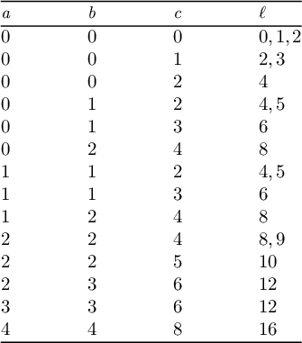
Corollary 1.8. Suppose $c \geqslant 2b$
and X does not satisfy the
$c \geqslant 2b$
and X does not satisfy the $K^2$
-total condition. Then X belongs to one of the
$K^2$
-total condition. Then X belongs to one of the $20$
families with
$20$
families with $a,b,c,\ell $
from the following table. In particular, if
$a,b,c,\ell $
from the following table. In particular, if $c \geqslant 2b$
, X satisfies the generality conditions, and X is not birationally rigid, then X belongs to one of these
$c \geqslant 2b$
, X satisfies the generality conditions, and X is not birationally rigid, then X belongs to one of these $20$
families.
$20$
families.
1.4 Convention
We denote numerical equivalence by $\equiv $
and use
$\equiv $
and use $\sim _{\mathbb {Q}}$
for linear equivalence of
$\sim _{\mathbb {Q}}$
for linear equivalence of $\mathbb {Q}$
-divisors. All varieties are algebraic, normal, and defined over
$\mathbb {Q}$
-divisors. All varieties are algebraic, normal, and defined over $\mathbb {C}$
unless stated otherwise. For a rational map
$\chi : Y \dashrightarrow X$
$\mathbb {C}$
unless stated otherwise. For a rational map
$\chi : Y \dashrightarrow X$
 , we denote the proper transform on Y of an object on X as $\chi ^{-1}_*(A)$
.
$\chi ^{-1}_*(A)$
.
2 Preliminary results: Singularities of pairs
In this section, we recall the notion of singularities of pairs. We also state some results which let us find relations between multiplicities and singularities.
Let X be an algebraic variety, possibly nonprojective and singular. Let E be a prime divisor on X. Then it is easy to associate a discrete valuation $\nu _E$
of
$\nu _E$
of $\mathbb {C}(X)$
corresponding to E by
$\mathbb {C}(X)$
corresponding to E by
 $$ \begin{align*} \nu_E(f)=\operatorname{mult}_E (f)\text{ for }f \in \mathbb{C}(X). \end{align*} $$
Definition 2.1 [Reference Pukhlikov27].
Let $\varphi :\widetilde {X}\to X$
be a projective birational morphism, and let
$\varphi :\widetilde {X}\to X$
be a projective birational morphism, and let $\nu $
be a discrete valuation of
$\nu $
be a discrete valuation of $\mathbb {C}(X)$
. We say that a triple
$\mathbb {C}(X)$
. We say that a triple $(\widetilde {X},\varphi ,E)$
is a realization of the discrete valuation
$(\widetilde {X},\varphi ,E)$
is a realization of the discrete valuation $\nu $
if E is a prime divisor on
$\nu $
if E is a prime divisor on $\widetilde {X}$
and
$\widetilde {X}$
and $\nu _E=\nu $
. Then
$\nu _E=\nu $
. Then $\varphi (E)$
is called the center of the discrete valuation
$\varphi (E)$
is called the center of the discrete valuation $\nu _E$
on X.
$\nu _E$
on X.
Note that if X is projective, then every discrete valuation of the field $\mathbb {C}(X)$
admits a center on X, which does not depend on the realization.
$\mathbb {C}(X)$
admits a center on X, which does not depend on the realization.
Definition 2.2. Let D be a $\mathbb {Q}$
-divisor on X. The multiplicity of a discrete valuation
$\mathbb {Q}$
-divisor on X. The multiplicity of a discrete valuation $\nu $
at D is
$\nu $
at D is
 $$ \begin{align*} \nu(D)=\operatorname{mult}_E \varphi^*(D) \in \mathbb{Q} \end{align*} $$
for some realization $(\widetilde {X},\varphi ,E)$
of
$(\widetilde {X},\varphi ,E)$
of $\nu $
. If the center of
$\nu $
. If the center of $\nu $
on X is of codimension
$\nu $
on X is of codimension $\geqslant 2$
, then we can write
$\geqslant 2$
, then we can write
 $$ \begin{align*} \varphi^*(D)=\varphi^{-1}_*(D)+\nu(D)E+\sum a_i E_i, \end{align*} $$
where $E_i$
are the exceptional divisors of
$E_i$
are the exceptional divisors of $\varphi $
that differ from E and
$\varphi $
that differ from E and $a_i\in \mathbb {Q}$
. It is important to note that the multiplicity does not depend on the choice of the realization.
$a_i\in \mathbb {Q}$
. It is important to note that the multiplicity does not depend on the choice of the realization.
Definition 2.3. Let D be a $\mathbb {Q}$
-divisor on X such that
$\mathbb {Q}$
-divisor on X such that $K_X+D$
is
$K_X+D$
is $\mathbb {Q}$
-Cartier. Let
$\mathbb {Q}$
-Cartier. Let $\pi :\widetilde {X}\to X$
be a birational morphism, and let
$\pi :\widetilde {X}\to X$
be a birational morphism, and let $\widetilde {D}=\pi ^{-1}_*(D)$
be the proper transform of D. Then
$\widetilde {D}=\pi ^{-1}_*(D)$
be the proper transform of D. Then
 $$ \begin{align*} K_{\widetilde{X}}+\widetilde{D}\sim\pi^*(K_X+D)+\sum_E a(E,X,D)E, \end{align*} $$
where E runs through all distinct exceptional divisors of $\pi $
on
$\pi $
on $\widetilde {X}$
and
$\widetilde {X}$
and $a(E,X,D)$
are rational numbers. The number
$a(E,X,D)$
are rational numbers. The number $a(E,X,D)$
=
$a(E,X,D)$
= $a(\nu _E,X,D)$
is called the discrepancy of the divisor E (discrete valuation
$a(\nu _E,X,D)$
is called the discrepancy of the divisor E (discrete valuation $\nu _E$
) with respect to the pair
$\nu _E$
) with respect to the pair $(X,D)$
.
$(X,D)$
.
Definition 2.4. Let D be a divisor on X. We say that the pair $(X,D)$
is terminal (resp. canonical) at a discrete valuation
$(X,D)$
is terminal (resp. canonical) at a discrete valuation $\nu $
with a center on X if
$\nu $
with a center on X if $a(E,X,D)>0$
(resp.
$a(E,X,D)>0$
(resp. $a(E,X,D)\geqslant 0$
) for some realization
$a(E,X,D)\geqslant 0$
) for some realization $(\widetilde {X},\varphi ,E)$
of
$(\widetilde {X},\varphi ,E)$
of $\nu $
. We say that the pair
$\nu $
. We say that the pair $(X,D)$
is terminal (resp. canonical) at a subvariety Z if it is terminal (resp. canonical) at every discrete valuation
$(X,D)$
is terminal (resp. canonical) at a subvariety Z if it is terminal (resp. canonical) at every discrete valuation $\nu $
on
$\nu $
on $K(X)$
such that a center of
$K(X)$
such that a center of $\nu $
on X is Z. We say that the pair
$\nu $
on X is Z. We say that the pair $(X,D)$
is terminal (resp. canonical) if it is terminal (resp. canonical) at every subvariety of codimension
$(X,D)$
is terminal (resp. canonical) if it is terminal (resp. canonical) at every subvariety of codimension $\geqslant 2$
. If
$\geqslant 2$
. If $D=0$
, we simply say that X has only terminal (resp. canonical) singularities.
$D=0$
, we simply say that X has only terminal (resp. canonical) singularities.
Definition 2.5. Let $\mathcal {M}$
be a linear system, not necessarily mobile, on X. We say that the pair
$\mathcal {M}$
be a linear system, not necessarily mobile, on X. We say that the pair $(X,\lambda \mathcal {M})$
is terminal (resp. canonical) if for every subvariety Z of codimension
$(X,\lambda \mathcal {M})$
is terminal (resp. canonical) if for every subvariety Z of codimension $\geqslant 2$
and for a general
$\geqslant 2$
and for a general $D\in \mathcal {M}$
, the pair
$D\in \mathcal {M}$
, the pair $(X,\lambda D)$
is terminal (resp. canonical) at Z.
$(X,\lambda D)$
is terminal (resp. canonical) at Z.
Remark 2.6. Consider the pair $(X,\mathcal {M})$
. Let
$(X,\mathcal {M})$
. Let $f:Y\to X$
be a projective birational morphism, let
$f:Y\to X$
be a projective birational morphism, let $E_i$
be the exceptional divisors of f, and let
$E_i$
be the exceptional divisors of f, and let $\widetilde {\mathcal {M}}$
be the proper transform of
$\widetilde {\mathcal {M}}$
be the proper transform of $\mathcal {M}$
on Y. Then
$\mathcal {M}$
on Y. Then
 $$ \begin{align*} K_Y+\widetilde{\mathcal{M}}-\sum a(E_i,X,\mathcal{M}) E_i\sim f^*(K_X+\mathcal{M}). \end{align*} $$
The pair
 $$ \begin{align*} \big(Y,\widetilde{\mathcal{M}}-\sum a(E_i,X,\mathcal{M}) E_i\big) \end{align*} $$
is called the log pullback of the pair $(X,\mathcal {M})$
. It follows from the definition that the log pullback of the pair has the same singularities as the pair. Note that we view
$(X,\mathcal {M})$
. It follows from the definition that the log pullback of the pair has the same singularities as the pair. Note that we view $\widetilde {\mathcal {M}}-\sum a(E_i,X,\mathcal {M}) E_i$
as a multiple of a linear system with fixed components.
$\widetilde {\mathcal {M}}-\sum a(E_i,X,\mathcal {M}) E_i$
as a multiple of a linear system with fixed components.
Lemma 2.7 [Reference Cheltsov9, Th. 1.8].
Let $\mathcal {M}$
be a mobile linear system on
$\mathcal {M}$
be a mobile linear system on $\mathbb {C}^2$
. Let C be a curve passing through the origin. Suppose the pair
$\mathbb {C}^2$
. Let C be a curve passing through the origin. Suppose the pair $(\mathbb {C}^2,\frac {1}{n}\mathcal {M}-\alpha C)$
is not canonical at
$(\mathbb {C}^2,\frac {1}{n}\mathcal {M}-\alpha C)$
is not canonical at $0$
, then for general
$0$
, then for general $D_1,D_2 \in \mathcal {M}$
,
$D_1,D_2 \in \mathcal {M}$
,
 $$ \begin{align*} \operatorname{mult}_0 D_1\cdot D_2> 4n^2\alpha. \end{align*} $$
Proposition 2.8 (Corti’s inequality [Reference Corti11, Th. 3.12]).
Let $\sum F_i \subset \mathbb {C}^3$
be a reduced surface. Let
$\sum F_i \subset \mathbb {C}^3$
be a reduced surface. Let $\mathcal {M}$
be a mobile linear system on
$\mathcal {M}$
be a mobile linear system on $\mathbb {C}^3$
, and let
$\mathbb {C}^3$
, and let $Z=D_1\cdot D_2$
be the intersection of general divisors
$Z=D_1\cdot D_2$
be the intersection of general divisors $D_1,D_2\in \mathcal {M}$
. Write
$D_1,D_2\in \mathcal {M}$
. Write $Z=Z_{h}+\sum Z_i$
, where the support of
$Z=Z_{h}+\sum Z_i$
, where the support of $Z_i$
is contained in
$Z_i$
is contained in $F_i$
and
$F_i$
and $Z_h$
intersects
$Z_h$
intersects $\sum F_i$
properly. Let
$\sum F_i$
properly. Let $\gamma _i> 0$
be rational numbers such that the pair
$\gamma _i> 0$
be rational numbers such that the pair $(\mathbb {C}^3,\frac {1}{n}\mathcal {M}-\sum \gamma _i F_i)$
is not canonical. Then there are positive rational numbers
$(\mathbb {C}^3,\frac {1}{n}\mathcal {M}-\sum \gamma _i F_i)$
is not canonical. Then there are positive rational numbers $0 < t_i \leqslant 1$
such that
$0 < t_i \leqslant 1$
such that
 $$ \begin{align*} \operatorname{mult}_0 Z_h + \sum t_i \operatorname{mult}_0 Z_i> 4n^2(1+\sum \gamma_i t_i\operatorname{mult}_0 F_i). \end{align*} $$
Remark 2.9. Decomposition of $Z=Z_h+\sum Z_i$
is not unique, but the inequality holds for any choice of the decomposition. Note that it is not a requirement that
$Z=Z_h+\sum Z_i$
is not unique, but the inequality holds for any choice of the decomposition. Note that it is not a requirement that $\sum F_i$
is a normal crossing divisor, nor do we ask the surfaces
$\sum F_i$
is a normal crossing divisor, nor do we ask the surfaces $F_i$
to be smooth.
$F_i$
to be smooth.
3 Rigidity of del Pezzo fibrations
3.1 Noether–Fano method for del Pezzo fibrations
Let us first describe the framework of proving birational rigidity for del Pezzo fibrations. Let $\pi : X \to \mathbb {P}^1$
be a del Pezzo fibration (satisfying
$\pi : X \to \mathbb {P}^1$
be a del Pezzo fibration (satisfying $K^2$
-condition), and let
$\chi \colon X \dashrightarrow Y$
$K^2$
-condition), and let
$\chi \colon X \dashrightarrow Y$
 be a birational map to a variety admitting a Mori fiber space $\pi _Y\colon Y\to Z$
. Let H be a very ample divisor on Y, and let
$\pi _Y\colon Y\to Z$
. Let H be a very ample divisor on Y, and let $\mathcal {M} = \chi ^{-1}_* (\big | H \big |)$
; we say that
$\mathcal {M} = \chi ^{-1}_* (\big | H \big |)$
; we say that $\mathcal {M}$
is a mobile linear system associated to
$\mathcal {M}$
is a mobile linear system associated to $\chi $
. There are nonnegative numbers
$\chi $
. There are nonnegative numbers $n \in \mathbb {Z}$
and
$n \in \mathbb {Z}$
and $l \in \mathbb {Q}$
such that
$l \in \mathbb {Q}$
such that $\mathcal {M} \subset \big | -n K_X + n l F \big |$
, where F is a fiber of
$\mathcal {M} \subset \big | -n K_X + n l F \big |$
, where F is a fiber of $\pi $
.
$\pi $
.
The core of the Noether–Fano method is the following. Suppose $\chi $
is not an isomorphism, then the pair
$\chi $
is not an isomorphism, then the pair $(X, \frac {1}{n} \mathcal {M})$
is not canonical. There are several possibilities for the centers of singularities of this pair: a singular point of X, a curve passing through a singular point of X, any other curve of X, and a nonsingular point of X. To prove X is birationally rigid, one uses the geometric properties of X to exclude a center or untwist
$(X, \frac {1}{n} \mathcal {M})$
is not canonical. There are several possibilities for the centers of singularities of this pair: a singular point of X, a curve passing through a singular point of X, any other curve of X, and a nonsingular point of X. To prove X is birationally rigid, one uses the geometric properties of X to exclude a center or untwist $\chi $
using that center. Excluding goes by proving that the pair is canonical at the center, and untwisting composes
$\chi $
using that center. Excluding goes by proving that the pair is canonical at the center, and untwisting composes $\chi $
with some square-birational map
$\chi $
with some square-birational map $\varphi \colon X\dashrightarrow X'$
, where
$\varphi \colon X\dashrightarrow X'$
, where $\chi \circ \varphi ^{-1}$
has lower Sarkisov degree than
$\chi \circ \varphi ^{-1}$
has lower Sarkisov degree than $\chi $
(see [Reference Corti11, §2.1] for the definition). Thus, the mobile linear system associated to
$\chi $
(see [Reference Corti11, §2.1] for the definition). Thus, the mobile linear system associated to $\chi \circ \varphi ^{-1}$
is less complicated, and the model X is replaced by
$\chi \circ \varphi ^{-1}$
is less complicated, and the model X is replaced by $X'$
.
$X'$
.
We do this analysis for orbifold del Pezzo fibrations of degree $2$
. Let X be a quasi-smooth hypersurface in a
$2$
. Let X be a quasi-smooth hypersurface in a $\mathbb {P}(1,1,1,2)$
-bundle over
$\mathbb {P}(1,1,1,2)$
-bundle over $\mathbb {P}^1$
. Suppose also that
$\mathbb {P}^1$
. Suppose also that $\pi : X \to \mathbb {P}^1$
is a del Pezzo fibration of degree
$\pi : X \to \mathbb {P}^1$
is a del Pezzo fibration of degree $2$
and that X satisfies the
$2$
and that X satisfies the $K^2$
-condition.
$K^2$
-condition.
3.2 Step 1: Curves not passing through singular locus of X
This part is well known by the work of Pukhlikov [Reference Pukhlikov28].
Proposition 3.1 [Reference Pukhlikov28, §3, Cases 2 and 4].
Let C be a curve on X which is not a section of $\pi $
. Suppose also that C does not pass through singular points of X. Then the pair
$\pi $
. Suppose also that C does not pass through singular points of X. Then the pair $(X,\frac {1}{n}\mathcal {M})$
is canonical at C.
$(X,\frac {1}{n}\mathcal {M})$
is canonical at C.
Proposition 3.2 [Reference Pukhlikov28, §3, Case 2].
Let C be a section of $\pi $
which does not pass through a singular point of X. Then either the pair
$\pi $
which does not pass through a singular point of X. Then either the pair $(X,\frac {1}{n}\mathcal {M})$
is canonical at C or there exists a birational involution
$(X,\frac {1}{n}\mathcal {M})$
is canonical at C or there exists a birational involution $\varphi _C$
such that
$\varphi _C$
such that
-
• there are numbers
$n^\prime <n$
and
$l^\prime $
such that
$\varphi _C(\mathcal {M})\subset \big | -n^\prime K_X +n^\prime l^\prime F \big |$
, and -
• the pair
$\big ( X, \frac {1}{n^\prime } (\varphi _C)(\mathcal {M}) \big )$
is canonical at C.


Corollary 3.3 [Reference Pukhlikov28, §3].
There is a birational map
$\varphi \colon X \dashrightarrow X$
 such that for the linear system $\varphi (\mathcal {M}) \subset \big | -n^\prime K_X + n^\prime l^\prime \big |$
, the pair
$\varphi (\mathcal {M}) \subset \big | -n^\prime K_X + n^\prime l^\prime \big |$
, the pair $(X,\frac {1}{n^\prime } \varphi (\mathcal {M}))$
is canonical at curves in
$(X,\frac {1}{n^\prime } \varphi (\mathcal {M}))$
is canonical at curves in $X \setminus \operatorname {Sing} X$
and
$X \setminus \operatorname {Sing} X$
and $\varphi = \varphi _{C_1} \circ \dots \circ \varphi _{C_m}$
, where
$\varphi = \varphi _{C_1} \circ \dots \circ \varphi _{C_m}$
, where $C_i$
are sections of X.
$C_i$
are sections of X.
Proof. Apply Proposition 3.1 and then apply Proposition 3.2 as many times as necessary. The process terminates since for every application of Proposition 3.2, we have $n^\prime < n$
.
$n^\prime < n$
.
In what follows, we write $\chi $
instead
$\chi $
instead $\chi \circ \varphi ^{-1}$
to simplify notation, and safely assume it is canonical at curves in the smooth locus. In the remainder of this article, we show that points and curves passing through singular points are either excluded or untwisted, as explained in the following steps.
$\chi \circ \varphi ^{-1}$
to simplify notation, and safely assume it is canonical at curves in the smooth locus. In the remainder of this article, we show that points and curves passing through singular points are either excluded or untwisted, as explained in the following steps.
3.3 Step 2: Singular points of X and curves passing through them
Singular points of X are cyclic quotient singularities. By the famous result of Kawamata on extremal extractions from such points, if the center of noncanonicity contains the singular point, then it is only that point and cannot be a curve (see §4). So it remains to study the singular points as centers. In §4, we construct birational maps to other models of del Pezzo fibration
$\varphi _I: X \dashrightarrow X_I$
 , with the diagram

being commutative. Let $\mathcal {M}_I \subset \big | -n K_{X_I} + n l_I F \big | $
be the linear system corresponding to the map
$\mathcal {M}_I \subset \big | -n K_{X_I} + n l_I F \big | $
be the linear system corresponding to the map $\chi \circ \varphi _I$
. We prove that the pair
$\chi \circ \varphi _I$
. We prove that the pair $(X_I, \frac {1}{n} \mathcal {M}_I)$
may only be noncanonical at nonsingular points of
$(X_I, \frac {1}{n} \mathcal {M}_I)$
may only be noncanonical at nonsingular points of $X_I$
for appropriate choice of I. Furthermore, we show that by construction
$X_I$
for appropriate choice of I. Furthermore, we show that by construction $X_I$
satisfies the generality conditions in the Main Theorem. This untwists
$X_I$
satisfies the generality conditions in the Main Theorem. This untwists $\chi $
for singular points. From that point on, with an abuse of notation, instead of
$\chi $
for singular points. From that point on, with an abuse of notation, instead of $\chi $
, we work with
$\chi $
, we work with $\chi \circ \varphi _I$
and call it
$\chi \circ \varphi _I$
and call it $\chi $
.
$\chi $
.
3.4 Step 3: Non-singular points of X
After Steps 1 and 2, we conclude that if $(X,\frac {1}{n}\mathcal {M})$
is not canonical at a subvariety B, then B is a point and X is smooth at B. This may indeed occur if
$(X,\frac {1}{n}\mathcal {M})$
is not canonical at a subvariety B, then B is a point and X is smooth at B. This may indeed occur if $\chi $
is square-birational. If we assume that
$\chi $
is square-birational. If we assume that $\chi $
is not square-birational, then we can use Proposition 5.1 to get a stronger requirement:
$\chi $
is not square-birational, then we can use Proposition 5.1 to get a stronger requirement: $(X,\frac {1}{n}\mathcal {M} - \gamma F)$
is not canonical at B, where F is a fiber containing B and
$(X,\frac {1}{n}\mathcal {M} - \gamma F)$
is not canonical at B, where F is a fiber containing B and $\gamma $
is a number depending on
$\gamma $
is a number depending on $\mathcal {M}$
. Recall that there are lines in the fibers that contain singular points of X which intersect
$\mathcal {M}$
. Recall that there are lines in the fibers that contain singular points of X which intersect $-K_X$
with
$-K_X$
with $\frac {1}{2}$
. If B does not lie on a such line, in particular, when F does not contain singularities of X, then Corti’s inequality together with Proposition 5.1 gives us the necessary contradiction to exclude B. This is the approach of [Reference Corti11], and we cover it in §5. Sections 6–8 are entirely devoted to the remaining case: excluding the possibility that the center is a nonsingular point on a curve in a fiber intersecting
$\frac {1}{2}$
. If B does not lie on a such line, in particular, when F does not contain singularities of X, then Corti’s inequality together with Proposition 5.1 gives us the necessary contradiction to exclude B. This is the approach of [Reference Corti11], and we cover it in §5. Sections 6–8 are entirely devoted to the remaining case: excluding the possibility that the center is a nonsingular point on a curve in a fiber intersecting $-K_X$
by
$-K_X$
by $\frac {1}{2}$
. As the reader expects, this is the most complicated case. We combine the approach of [Reference Corti11] with the staircase used for cubic fibrations in [Reference Pukhlikov28, §§6 and 7] to exclude these nonsingular points.
$\frac {1}{2}$
. As the reader expects, this is the most complicated case. We combine the approach of [Reference Corti11] with the staircase used for cubic fibrations in [Reference Pukhlikov28, §§6 and 7] to exclude these nonsingular points.
4 Square maps from
$\frac {1}{2}(1,1,1)$
-points

In this section, we explicitly work out the square-birational maps produced by blowing up the singular points. Let X be the hypersurface of bi-degree $(\ell ,4)$
given by the equation
$(\ell ,4)$
given by the equation
 $$ \begin{align*}f(u,v) w^2 + q(x,y,z;u,v) w + r(x,y,z;u,v)=0 \end{align*} $$
in the toric variety $T=\mathbb {P}(1_x,1_y,1_z,2_w)_{(0,a,b,c)}/\mathbb {P}^1_{u:v}$
.
$T=\mathbb {P}(1_x,1_y,1_z,2_w)_{(0,a,b,c)}/\mathbb {P}^1_{u:v}$
.
4.1 Simple case: X has one singular point
First, for simplicity, suppose $f(u,v)=u$
. Then the fiber F given by
$f(u,v)=u$
. Then the fiber F given by $u = 0$
contains the singular point of X. We now describe each map of the following diagram:
$u = 0$
contains the singular point of X. We now describe each map of the following diagram:

The variety U is the open subset of X given by $v \neq 0$
. It can be viewed as the locus
$v \neq 0$
. It can be viewed as the locus $\{f(u,1) w^2 + q(x,y,z;u,1) w + r(x,y,z;u,1)=0\}$
inside
$\{f(u,1) w^2 + q(x,y,z;u,1) w + r(x,y,z;u,1)=0\}$
inside $\mathbb {P}(1_x,1_y,1_z,2_w)\times \mathbb {C}^1_u$
. The map
$\mathbb {P}(1_x,1_y,1_z,2_w)\times \mathbb {C}^1_u$
. The map $\sigma $
is the Kawamata blowup of U along the
$\sigma $
is the Kawamata blowup of U along the $\frac {1}{2}(1,1,1)$
-point [Reference Kawamata20]. We may describe
$\frac {1}{2}(1,1,1)$
-point [Reference Kawamata20]. We may describe $\widetilde {U}$
as a hypersurface in
$\widetilde {U}$
as a hypersurface in $\widetilde {V}$
, where
$\widetilde {V}$
, where $\widetilde {V}$
is a quasi-projective toric variety with
$\widetilde {V}$
is a quasi-projective toric variety with $\operatorname {Cox} \widetilde {V} = \mathbb {C}[x,y,z,w,u,\bar {u}]$
. The grading of this ring is given by the matrix
$\operatorname {Cox} \widetilde {V} = \mathbb {C}[x,y,z,w,u,\bar {u}]$
. The grading of this ring is given by the matrix
 $$ \begin{align*}\left(\begin{array}{ccccccc} u & x & y & z & w & \bar{u} \\ 0 & 1 & 1 & 1 & 2 & 0 \\ 2 & 1 & 1 & 1 & 0 & -2 \end{array}\right) \end{align*} $$
and irrelevant ideal $(u,x,y,z)\cap (w,\bar {u})\cap (x,y,z,w)$
(see [Reference Ahmadinezhad3, §3.2] for a general treatment of Cox rings of blowups of rank 2 toric varieties). Note that we are looking at the open set
$(u,x,y,z)\cap (w,\bar {u})\cap (x,y,z,w)$
(see [Reference Ahmadinezhad3, §3.2] for a general treatment of Cox rings of blowups of rank 2 toric varieties). Note that we are looking at the open set $\{v\neq 0\}$
, and hence the rank drops to 2 and the ideal simplifies. We may well-form [Reference Ahmadinezhad3, §2] the matrix above and rewrite it as
$\{v\neq 0\}$
, and hence the rank drops to 2 and the ideal simplifies. We may well-form [Reference Ahmadinezhad3, §2] the matrix above and rewrite it as
 $$ \begin{align*}\left(\begin{array}{ccccccc} u & x & y & z & w & \bar{u} \\ 0 & 1 & 1 & 1 & 2 & 0 \\ -1 & 0 & 0 & 0 & 1 & 1 \end{array}\right). \end{align*} $$
The equation of $\widetilde {U}$
is
$\widetilde {U}$
is
 $$ \begin{align*}u w^2 + q(x,y,z; \bar{u} u) w + \bar{u} r(x,y,z; \bar{u} u)=0, \end{align*} $$
where $q(x,y,z; u) = q(y,x,z; u,1)$
and
$q(x,y,z; u) = q(y,x,z; u,1)$
and $r(x,y,z;u)=r(x,y,z;u,1)$
. To produce a Sarkisov link on
$r(x,y,z;u)=r(x,y,z;u,1)$
. To produce a Sarkisov link on $\widetilde {U}$
, we run a 2-ray game on the ambient space (
$\widetilde {U}$
, we run a 2-ray game on the ambient space ( $\widetilde {V}$
to begin with) and restrict it to the threefold [Reference Ahmadinezhad and Zucconi5]. Note that the 2-ray game corresponds to the variation of Geometric Invariant Theory (GIT), inevitably changing
$\widetilde {V}$
to begin with) and restrict it to the threefold [Reference Ahmadinezhad and Zucconi5]. Note that the 2-ray game corresponds to the variation of Geometric Invariant Theory (GIT), inevitably changing $(u,x,y,z)\cap (w,\bar {u})$
part in the irrelevant ideal. The component
$(u,x,y,z)\cap (w,\bar {u})$
part in the irrelevant ideal. The component $(x,y,z,w)$
in the ideal remains unchanged, and preserves the fibers (the 2-ray game is relative over the base of the fibration). The first step of the game on
$(x,y,z,w)$
in the ideal remains unchanged, and preserves the fibers (the 2-ray game is relative over the base of the fibration). The first step of the game on $\widetilde {V}$
does not produce a 2-ray game on
$\widetilde {V}$
does not produce a 2-ray game on $\widetilde {U}$
, caused by the fact that the equation of the hypersurface belongs to the irrelevant component
$\widetilde {U}$
, caused by the fact that the equation of the hypersurface belongs to the irrelevant component $(w,\bar {u})$
, and hence we are forced to do an unprojection (preserving
$(w,\bar {u})$
, and hence we are forced to do an unprojection (preserving $\widetilde {U}$
). This embeds
$\widetilde {U}$
). This embeds $\widetilde {U}$
in the toric variety defined by the Cox ring
$\widetilde {U}$
in the toric variety defined by the Cox ring $\mathbb {C}[x,y,z,w,u,\bar {u}]$
graded by
$\mathbb {C}[x,y,z,w,u,\bar {u}]$
graded by
 $$ \begin{align*}\left(\begin{array}{cccccccc} u & t & x & y & z & w & \bar{u} \\ 0 & 2 & 1 & 1 & 1 & 2 & 0 \\ -1 & -1 & 0 & 0 & 0 & 1 & 1 \end{array}\right). \end{align*} $$
The irrelevant ideal is $(u,t,x,y,z)\cap (w,\bar {u})\cap (x,y,z,w,t)$
, and
$(u,t,x,y,z)\cap (w,\bar {u})\cap (x,y,z,w,t)$
, and $\widetilde {U}$
is a complete intersection of two hypersurfaces:
$\widetilde {U}$
is a complete intersection of two hypersurfaces:
 $$ \begin{align*}u w + q(x,y,z; \bar{u} u) = \bar{u}t \quad\text{and}\quad -wt=r(x,y,z; \bar{u} u). \end{align*} $$
The toric 2-ray game now restricts to a 2-ray game on $\widetilde {U}$
. The first step is the flop of eight lines, which corresponds to the eight solutions of
$\widetilde {U}$
. The first step is the flop of eight lines, which corresponds to the eight solutions of $\{q(x,y,z,0)=r(x,y,z,0)=0\}\subset \mathbb {P}^2$
, mapping
$\{q(x,y,z,0)=r(x,y,z,0)=0\}\subset \mathbb {P}^2$
, mapping $\widetilde {U}$
to
$\widetilde {U}$
to $\bar {U}$
by crossing the
$\bar {U}$
by crossing the $(1,0)$
wall. Recall that the solutions of
$(1,0)$
wall. Recall that the solutions of $\{q(x,y,z,0)=r(x,y,z,0)=0\}$
are distinct because of the generality conditions in the Main Theorem.
$\{q(x,y,z,0)=r(x,y,z,0)=0\}$
are distinct because of the generality conditions in the Main Theorem.
The map $\bar {\sigma }$
is defined as
$\bar {\sigma }$
is defined as
 $$ \begin{align*}(x,y,z,w,t,u,\bar{u}) \mapsto (u^{\frac{1}{2}}x,u^{\frac{1}{2}}y, u^{\frac{1}{2}}z, w, u t, u \bar{u}). \end{align*} $$
It contracts the proper transform of F into a $\frac {1}{2}(1,1,1)$
-point. Thus, we see that the equations of the image of
$\frac {1}{2}(1,1,1)$
-point. Thus, we see that the equations of the image of $\bar {\sigma }$
are
$\bar {\sigma }$
are
 $$ \begin{align*}\bar{u} t = w + q(x,y,z; \bar{u}) \quad\text{and}\quad w t + r(x,y,z; \bar{u}) = 0. \end{align*} $$
We can eliminate the variable w, and thus we have only one equation
 $$ \begin{align*}\bar{u} t^2 - q(x,y,z;\bar{u}) w + r(x,y,z;\bar{u})=0. \end{align*} $$
Clearly, this variety is isomorphic to U. Thus, the map $\varphi $
is a birational automorphism. We may write the map
$\varphi $
is a birational automorphism. We may write the map $\varphi $
in coordinates as
$\varphi $
in coordinates as
 $$ \begin{align*}(x,y,z,w,u) \mapsto \left(x,y,z,-w+\frac{q(x,y,z;u)}{u};u \right). \end{align*} $$
In particular, we see that $\varphi $
is a local involution.
$\varphi $
is a local involution.
4.2 Birational models of X: Square-birational maps
Note that the description of maps and models in the simple case in §4.1 works out for any calculations around the local ring near the point in the image of the singular point at the base curve. We use this to describe all models $X_I$
.
$X_I$
.
Embed X into V, a toric $\mathbb {P}(1,1,1,2,2)$
-bundle over
$\mathbb {P}(1,1,1,2,2)$
-bundle over $\mathbb {P}^1$
, as a complete intersection as follows. Let N be the degree of
$\mathbb {P}^1$
, as a complete intersection as follows. Let N be the degree of $f \in \mathbb {C}[u,v]$
. Let the weight matrix of the toric variety V be
$f \in \mathbb {C}[u,v]$
. Let the weight matrix of the toric variety V be
 $$ \begin{align*}\left(\begin{array}{ccccccc} v & u & x & y & z & w & s \\ 0 & 0 & 1 & 1 & 1 & 2 & 2 \\ 1 & 1 & 0 & a & b & c & c+N \end{array}\right) \end{align*} $$
with irrelevant ideal $(u,v)\cap (x,y,z,w,s)$
, and suppose the equations of X are
$(u,v)\cap (x,y,z,w,s)$
, and suppose the equations of X are
 $$ \begin{align*} &s = f(u,v) w + q(x,y,z;u,v), &s w + r(x,y,z;u,v) = 0. \end{align*} $$
Note that the variable s can be eliminated altogether using the first equation, and then what we are left with is the model presented in §1.3.
The quasi-smoothness of X implies that f has N distinct zeros, and hence it can be written in the form $f(u,v) = l_1(u,v) \dots l_N(u,v)$
, a product of distinct linear forms.
$f(u,v) = l_1(u,v) \dots l_N(u,v)$
, a product of distinct linear forms.
Following the Sarkisov link described in §4.1, we can construct $X_{\{1\}}$
, the variety obtained at the end of the Sarkisov link starting from the Kawamata blowup of the singular point in the fiber
$X_{\{1\}}$
, the variety obtained at the end of the Sarkisov link starting from the Kawamata blowup of the singular point in the fiber $l_1=0$
:
$l_1=0$
:
The threefold $X_{\{1\}}$
is defined as a complete intersection defined by equations
$X_{\{1\}}$
is defined as a complete intersection defined by equations
 $$ \begin{align*}l_1s = l_2\dots l_N w + q(x,y,z;u,v) \quad\text{and}\quad s w + r(x,y,z;u,v) = 0 \end{align*} $$
in the toric fivefold $V_1$
with grading
$V_1$
with grading
 $$ \begin{align*}\left(\begin{array}{ccccccc} v & u & x & y & z & w & s \\ 0 & 0 & 1 & 1 & 1 & 2 & 2 \\ 1 & 1 & 0 & a & b & c+1 & c+N-1 \end{array}\right). \end{align*} $$
Note that the irrelevant ideal remains unchanged. Similarly, $X_I\subset V_{\big | I \big |}$
is defined by
$X_I\subset V_{\big | I \big |}$
is defined by
 $$ \begin{align*} \prod_{i \in I} l_i s = \prod_{j \not\in I} l_j w + q(x,y,z;u,v) \quad\text{and}\quad s w + r(x,y,z;u,v) = 0, \end{align*} $$
where $V_{\big | I \big |}$
is graded by
$V_{\big | I \big |}$
is graded by
 $$ \begin{align*}\left(\begin{array}{ccccccc} v & u & x & y & z & w & s \\ 0 & 0 & 1 & 1 & 1 & 2 & 2 \\ 1 & 1 & 0 & a & b & c + \big|I\big| & c + N - \big|I\big| \end{array}\right). \end{align*} $$
At last, we denote by $\pi _I: X_I \to \mathbb {P}^1_{u,v}$
the restriction of the projection
$\pi _I: X_I \to \mathbb {P}^1_{u,v}$
the restriction of the projection $V_{\big | I \big |} \to \mathbb {P}^1_{u,v}$
.
$V_{\big | I \big |} \to \mathbb {P}^1_{u,v}$
.
While this defines the birational maps between, say, $X_I$
and
$X_I$
and $X_{I\cup \{j\}}$
for
$X_{I\cup \{j\}}$
for $j\notin I$
, the description of this birational map as an elementary Sarkisov link is identical to the case in §4.1, after a suitable change of coordinates.
$j\notin I$
, the description of this birational map as an elementary Sarkisov link is identical to the case in §4.1, after a suitable change of coordinates.
Remark 4.1. The extremal contraction $\widetilde {X} \to X$
is constructed so that the image of the exceptional locus is a terminal quotient singularity [Reference Kawamata20, Th. 5], and locally is the Kawamata blowup of that point. This is a unique extremal extraction according to Kawamata. Then the 2-ray game is followed by a simple Atiyah flop, in particular, it does not change the singularities of
$\widetilde {X} \to X$
is constructed so that the image of the exceptional locus is a terminal quotient singularity [Reference Kawamata20, Th. 5], and locally is the Kawamata blowup of that point. This is a unique extremal extraction according to Kawamata. Then the 2-ray game is followed by a simple Atiyah flop, in particular, it does not change the singularities of $\widetilde {X}$
. In short, the links we described here are unique elementary Sarkisov links starting at
$\widetilde {X}$
. In short, the links we described here are unique elementary Sarkisov links starting at $\frac {1}{2}(1,1,1)$
-points, and, as it can be seen from the coordinate description of the birational map, the links we constructed are birational involutions in analytic neighborhood of the central fiber. In particular, it follows that
$\frac {1}{2}(1,1,1)$
-points, and, as it can be seen from the coordinate description of the birational map, the links we constructed are birational involutions in analytic neighborhood of the central fiber. In particular, it follows that $\pi _I: X_I \to \mathbb {P}^1_{u,v}$
is a del Pezzo fibration.
$\pi _I: X_I \to \mathbb {P}^1_{u,v}$
is a del Pezzo fibration.
Remark 4.2. It is clear from the symmetric equation of $X_I$
described above that
$X_I$
described above that $X_I\cong X_{J}$
, where
$X_I\cong X_{J}$
, where $J=\{1,\dots ,N\}\backslash I$
. Furthermore, in particular,
$J=\{1,\dots ,N\}\backslash I$
. Furthermore, in particular, $X_{\{1,\dots ,N\}}\cong X$
.
$X_{\{1,\dots ,N\}}\cong X$
.
4.3 Canonicity at
$\frac {1}{2}(1,1,1)$
-point

Let $\mathcal {M} \subset \big | -n K_X + l F \big |$
be the mobile linear system associated to a birational map
$\chi \colon X \dashrightarrow Y$
$\mathcal {M} \subset \big | -n K_X + l F \big |$
be the mobile linear system associated to a birational map
$\chi \colon X \dashrightarrow Y$
 to a total space Y of a Mori fiber space. Let $\mathcal {M}_I$
be the proper transform of
$\mathcal {M}_I$
be the proper transform of $\mathcal {M}$
on
$\mathcal {M}$
on $X_I$
. We now prove that there is an
$X_I$
. We now prove that there is an $I \subset \{1,\dots ,N\}$
for which the linear system
$I \subset \{1,\dots ,N\}$
for which the linear system $\mathcal {M}_I$
is canonical at
$\mathcal {M}_I$
is canonical at $\frac {1}{2}(1,1,1)$
-points and at curves passing through them.
$\frac {1}{2}(1,1,1)$
-points and at curves passing through them.
Proposition 4.3 [Reference Kawamata20, Th. 5].
Let $g:\widetilde {X}\to X$
be the blowup at a
$g:\widetilde {X}\to X$
be the blowup at a $\frac {1}{2}(1,1,1)$
-point Q, let D be an effective
$\frac {1}{2}(1,1,1)$
-point Q, let D be an effective $\mathbb {Q}$
-divisor on X, and let
$\mathbb {Q}$
-divisor on X, and let $E_Q$
be the exceptional divisor of g. Then a pair
$E_Q$
be the exceptional divisor of g. Then a pair $(X,D)$
is canonical at Q if and only if it is canonical at
$(X,D)$
is canonical at Q if and only if it is canonical at $\nu _{E_Q}$
, that is,
$\nu _{E_Q}$
, that is, $a(E_Q,X,D) \geqslant 0$
.
$a(E_Q,X,D) \geqslant 0$
.
Corollary 4.4. Suppose the pair $(X,D)$
is not canonical at a curve C passing through the
$(X,D)$
is not canonical at a curve C passing through the $\frac {1}{2}(1,1,1)$
-point Q. Then the pair
$\frac {1}{2}(1,1,1)$
-point Q. Then the pair $(X,D)$
is not canonical at Q.
$(X,D)$
is not canonical at Q.
Because of this corollary, we only concentrate on $\frac {1}{2}(1,1,1)$
being the center of noncanonicity. Note that it is possible for the pair
$\frac {1}{2}(1,1,1)$
being the center of noncanonicity. Note that it is possible for the pair $(X,\frac {1}{n} \mathcal {M})$
to be noncanonical at a singular point of X. What is true, and proved here, is that there always exist a model
$(X,\frac {1}{n} \mathcal {M})$
to be noncanonical at a singular point of X. What is true, and proved here, is that there always exist a model $X_I$
of X for which the pair
$X_I$
of X for which the pair $(X_I,\frac {1}{n} \mathcal {M}_I)$
is canonical at singular points.
$(X_I,\frac {1}{n} \mathcal {M}_I)$
is canonical at singular points.
Proposition 4.5. Let $\pi : X \to \mathbb {P}^1$
be a del Pezzo fibration as in the Main Theorem. Let
$\pi : X \to \mathbb {P}^1$
be a del Pezzo fibration as in the Main Theorem. Let $\mathcal {M} \subset \big | -n K_X + l F \big |$
be the mobile linear system associated to a birational map
$\chi \colon X \dashrightarrow Y$
$\mathcal {M} \subset \big | -n K_X + l F \big |$
be the mobile linear system associated to a birational map
$\chi \colon X \dashrightarrow Y$
 to the total space Y of a Mori fiber space. Denote singular points of X by $Q_1,\dots ,Q_N$
. Let
$Q_1,\dots ,Q_N$
. Let $I \subset \{1,\dots ,N\}$
be the maximal subset of indices such that the pair
$I \subset \{1,\dots ,N\}$
be the maximal subset of indices such that the pair $(X, \frac {1}{n} \mathcal {M})$
is not canonical at
$(X, \frac {1}{n} \mathcal {M})$
is not canonical at $Q_i$
for
$Q_i$
for $i \in I$
. Let
$i \in I$
. Let $\mathcal {M}_I$
be the proper transform of
$\mathcal {M}_I$
be the proper transform of $\mathcal {M}$
on
$\mathcal {M}$
on $X_I$
. Then the pair
$X_I$
. Then the pair $(X_I, \frac {1}{n} \mathcal {M}_I)$
is canonical at all singular points of
$(X_I, \frac {1}{n} \mathcal {M}_I)$
is canonical at all singular points of $X_I$
.
$X_I$
.
Proof. We prove it for $I = \{1\}$
, and the rest follows by induction. Suppose
$I = \{1\}$
, and the rest follows by induction. Suppose $\varphi \colon X\dashrightarrow X'=X_I$
is the birational transform described earlier starting from the blowup of the
$\varphi \colon X\dashrightarrow X'=X_I$
is the birational transform described earlier starting from the blowup of the $\frac {1}{2}$
point
$\frac {1}{2}$
point $Q_1$
, which factors as
$Q_1$
, which factors as

with f and $f_I$
being the Kawamata blowups of the singular points and
$f_I$
being the Kawamata blowups of the singular points and $\psi $
the flopping map between
$\psi $
the flopping map between $\widetilde {X}$
and
$\widetilde {X}$
and $\widetilde {X_I}$
. We have the following relations:
$\widetilde {X_I}$
. We have the following relations:
 $$\begin{align*}\mathcal{M}\sim -n K_X + l F\quad\text{and}\quad \mathcal{M}_I\sim-n K_{X_I} + l_I F_I,\end{align*}$$
 $$\begin{align*}\widetilde{\mathcal{M}}=f^*\mathcal{M}-\nu E\quad\text{and}\quad \widetilde{\mathcal{M}_I}=g^*\mathcal{M}-\nu_I E_I,\end{align*}$$
 $$\begin{align*}f^*F = f_*^{-1} F + E \quad\text{and}\quad f_I^*F_I = (f_I)_*^{-1} F_I + E_I ,\end{align*}$$
where E and $E_I$
are the exceptional divisors of f and
$E_I$
are the exceptional divisors of f and $f_I$
, and
$f_I$
, and $\widetilde {\mathcal {M}}$
and
$\widetilde {\mathcal {M}}$
and $\widetilde {\mathcal {M}_I}$
are the strict transforms of
$\widetilde {\mathcal {M}_I}$
are the strict transforms of $\mathcal {M}$
and
$\mathcal {M}$
and $\mathcal {M}_I$
with multiplicities
$\mathcal {M}_I$
with multiplicities $\nu $
,
$\nu $
, $\nu _I$
positive integers.
$\nu _I$
positive integers.
Let $g\colon V \to \widetilde {X}$
and
$g\colon V \to \widetilde {X}$
and $h\colon V \to \widetilde {X_I}$
be the resolution of the flopping map
$h\colon V \to \widetilde {X_I}$
be the resolution of the flopping map $\psi $
. Denote
$\psi $
. Denote
 $$\begin{align*}F_V = (f\circ g)^*(F) = (f_I\circ h)^*(F_I), \quad \text{and} \quad \mathcal{M}_V = (f\circ g)_*^{-1}(\mathcal{M}) = (f_I\circ h)_*^{-1}(\mathcal{M}_I). \end{align*}$$
Then we have the following equivalence:
 $$ \begin{align*} l F_V + \left(\frac{1}{2} - \frac{\nu}{n}\right) g_*^{-1}(E) + \sum a_i E_i \sim K_V + \frac{1}{n} \mathcal{M}_V\sim l_I F_V + \left(\frac{1}{2} - \frac{\nu_I}{n}\right) h_*^{-1}(E_I) + \sum b_i E_i \end{align*} $$
for some rational $a_i$
and
$a_i$
and $b_i$
. Since
$b_i$
. Since $\psi $
is small, the divisors
$\psi $
is small, the divisors $E_i$
in the sums on the left-hand side and on the right-hand side are the same. We rearrange the terms:
$E_i$
in the sums on the left-hand side and on the right-hand side are the same. We rearrange the terms:
 $$ \begin{align} (l-l_I)F_V \sim \left(\frac{1}{2}-\frac{\nu_I}{n}\right)h_*^{-1}(E_I)+ \left(\frac{\nu}{n}-\frac{1}{2} \right)g_*^{-1}(E) + \sum (b_i - a_i) E_i. \end{align} $$
On the other hand, we have
 $$ \begin{align} F_V \sim g_*^{-1}(E)+ h_*^{-1}(E_I) + \sum c_i E_i \end{align} $$
for some $c_i$
.
$c_i$
.
It follows from linear independence of $E_i, g_*^{-1}(E), h_*^{-1}(E_I)$
that equivalences (1) and (2) are proportional, in particular, we have
$E_i, g_*^{-1}(E), h_*^{-1}(E_I)$
that equivalences (1) and (2) are proportional, in particular, we have
 $$\begin{align*}\nu + \nu_I = n. \end{align*}$$
It implies that at most one of $(X, \frac {1}{n} \mathcal {M})$
and
$(X, \frac {1}{n} \mathcal {M})$
and $(X_I, \frac {1}{n} \mathcal {M}_I)$
can be noncanonical at those particular singular points.
$(X_I, \frac {1}{n} \mathcal {M}_I)$
can be noncanonical at those particular singular points.
Remark 4.6. Note that $\mathcal {M}_I \subset \big |-n K_{X_I} + l_I F_I \big |$
for some
$\mathcal {M}_I \subset \big |-n K_{X_I} + l_I F_I \big |$
for some $l_I$
, that is, n does not change. This is the case since the maps
$l_I$
, that is, n does not change. This is the case since the maps $\varphi _I$
induce isomorphisms on general fibers.
$\varphi _I$
induce isomorphisms on general fibers.
Lemma 4.7. All the varieties $X_I$
satisfy the generality conditions in the Main Theorem.
$X_I$
satisfy the generality conditions in the Main Theorem.
Proof. The maps $\varphi _I$
are compositions of maps
$\varphi _I$
are compositions of maps $\varphi _i$
, where the map
$\varphi _i$
, where the map $\varphi _i$
is a birational involution of the analytical neighborhood of the fiber containing
$\varphi _i$
is a birational involution of the analytical neighborhood of the fiber containing $Q_i$
. Thus, the fibers, containing singularities on
$Q_i$
. Thus, the fibers, containing singularities on $X_I$
, are isomorphic to the fibers containing singularities on X. Note that quasi-smoothness of
$X_I$
, are isomorphic to the fibers containing singularities on X. Note that quasi-smoothness of $X_I$
can be checked explicitly. The ambient space is singular along the surface
$X_I$
can be checked explicitly. The ambient space is singular along the surface $\{x=y=z=0\}$
, which is a
$\{x=y=z=0\}$
, which is a $\mathbb {P}(2,2)$
-bundle over
$\mathbb {P}(2,2)$
-bundle over $\mathbb {P}^1$
. This is cut out by X at the solutions to
$\mathbb {P}^1$
. This is cut out by X at the solutions to $sw=(\prod _{i \in I} l_i)s - (\prod _{j \not \in I} l_j) w=0\}$
, which is a finite set of points. Locally near each singular point s or w, as well as a local parameter in the base, appears as linear term (because
$sw=(\prod _{i \in I} l_i)s - (\prod _{j \not \in I} l_j) w=0\}$
, which is a finite set of points. Locally near each singular point s or w, as well as a local parameter in the base, appears as linear term (because $l_i$
’s are distinct), and hence can be eliminated so that the analytic type of singularity at each point is
$l_i$
’s are distinct), and hence can be eliminated so that the analytic type of singularity at each point is $\frac {1}{2}(1,1,1)$
. There are no other singularities by the generality assumptions on X.
$\frac {1}{2}(1,1,1)$
. There are no other singularities by the generality assumptions on X.
5 Supermaximal singularities
In this section, we establish a framework for excluding smooth points. We follow the approach of Pukhlikov [Reference Pukhlikov28]. We exclude the points that lie on $\pi $
-vertical curves intersecting
$\pi $
-vertical curves intersecting $-K_X$
by
$-K_X$
by $\frac {1}{2}$
in §6–8, and all the other points in Proposition 5.4.
$\frac {1}{2}$
in §6–8, and all the other points in Proposition 5.4.
By Corollary 3.3, we may assume that the pair $(X, \frac {1}{n} \mathcal {M})$
is canonical at curves in the smooth locus. In §§3 and 4, we have shown that there is a model
$(X, \frac {1}{n} \mathcal {M})$
is canonical at curves in the smooth locus. In §§3 and 4, we have shown that there is a model $X_I$
for which the pair
$X_I$
for which the pair $(X_I, \frac {1}{n} \mathcal {M}_I)$
is canonical at all the singularities of
$(X_I, \frac {1}{n} \mathcal {M}_I)$
is canonical at all the singularities of $X_I$
. By Corollary 4.4, the pair
$X_I$
. By Corollary 4.4, the pair $(X_I, \frac {1}{n} \mathcal {M}_I)$
is also canonical at curves passing through the singular locus of
$(X_I, \frac {1}{n} \mathcal {M}_I)$
is also canonical at curves passing through the singular locus of $X_I$
. Thus, if the pair
$X_I$
. Thus, if the pair $(X_I, \frac {1}{n} \mathcal {M}_I)$
is not canonical at B, then B is a point and X is smooth at B. This allows us to use the following result.
$(X_I, \frac {1}{n} \mathcal {M}_I)$
is not canonical at B, then B is a point and X is smooth at B. This allows us to use the following result.
Proposition 5.1 [Reference Okada26, Prop. 2.7].
Let $\pi : X \to \mathbb {P}^1$
be a del Pezzo fibration. Suppose that we are given a nonsquare-birational map
$\chi \colon X \dashrightarrow Y$
$\pi : X \to \mathbb {P}^1$
be a del Pezzo fibration. Suppose that we are given a nonsquare-birational map
$\chi \colon X \dashrightarrow Y$
 to a Mori fiber space $\pi _Y \colon Y \to Z$
, and let
$\pi _Y \colon Y \to Z$
, and let $\mathcal {M} \subset \big | -nK_X + l n F\big |$
be a mobile linear system associated to
$\mathcal {M} \subset \big | -nK_X + l n F\big |$
be a mobile linear system associated to $\chi $
. Suppose in addition that the pair
$\chi $
. Suppose in addition that the pair $(X, \frac {1}{n} \mathcal {M})$
is canonical at curves on X and
$(X, \frac {1}{n} \mathcal {M})$
is canonical at curves on X and $l \geqslant 0$
. Then there exist divisorial valuations
$l \geqslant 0$
. Then there exist divisorial valuations $\nu _i$
centered at points
$\nu _i$
centered at points $P_1,\dots ,P_k$
of X contained in distinct
$P_1,\dots ,P_k$
of X contained in distinct $\pi $
-fibers and there exist positive rational numbers
$\pi $
-fibers and there exist positive rational numbers $\gamma _1,\dots ,\gamma _k$
with the following properties:
$\gamma _1,\dots ,\gamma _k$
with the following properties:
-
•
$(X,\frac {1}{n} \mathcal {M} - \sum \gamma _j F_j)$
is not canonical at
$\nu _1,\dots ,\nu _k$
, where
$F_i$
is the
$\pi $
-fiber containing
$P_i$
. -
•
$\sum _{j=1}^{k} \gamma _j> l$
.


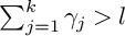
We combine this proposition with Corti’s inequality to derive a contradiction from the existence of a nonsquare-birational map
$\chi \colon X \dashrightarrow Y$
 . Note that $l \geqslant 0$
since
$l \geqslant 0$
since $X_I$
satisfies the
$X_I$
satisfies the $K^2$
-condition. This is why we require the total
$K^2$
-condition. This is why we require the total $K^2$
-condition in the Main Theorem.
$K^2$
-condition in the Main Theorem.
We now introduce the notions and notations necessary for application of Corti’s inequality. First, we simplify the notations by dropping the index I, that is, from now on, we denote $X_I$
by X,
$X_I$
by X, $\pi _I$
by
$\pi _I$
by $\pi $
, and so forth.
$\pi $
, and so forth.
Let $D_1$
,
$D_1$
, $D_2\in \mathcal {M}$
be general members, and consider the effective
$D_2\in \mathcal {M}$
be general members, and consider the effective $1$
-cycle
$1$
-cycle $Z=D_1\cdot D_2$
. For some point P, we find an upper bound on
$Z=D_1\cdot D_2$
. For some point P, we find an upper bound on $\operatorname {mult}_P Z$
using the degrees and a lower bound using Corti’s inequality.
$\operatorname {mult}_P Z$
using the degrees and a lower bound using Corti’s inequality.
We decompose $Z=Z^v+Z^h$
into the vertical and horizontal components with relation to the fibration
$Z=Z^v+Z^h$
into the vertical and horizontal components with relation to the fibration $\pi $
. For the vertical components, we have the decomposition
$\pi $
. For the vertical components, we have the decomposition
 $$ \begin{align*} Z^v=\sum_{t\in \mathbb{P}^1}Z^v_i + Z^{\prime}, \end{align*} $$
where the support of $Z^v_i$
is contained in
$Z^v_i$
is contained in $F_i$
from Proposition 5.1 and the support of
$F_i$
from Proposition 5.1 and the support of $Z^\prime $
is disjoint from
$Z^\prime $
is disjoint from $F_1,\dots ,F_k$
. We define the degree of a vertical
$F_1,\dots ,F_k$
. We define the degree of a vertical $1$
-cycle
$1$
-cycle $C^v$
by the number
$C^v$
by the number $\deg C^v=C^v\cdot (-K_X)$
and the degree of a horizontal
$\deg C^v=C^v\cdot (-K_X)$
and the degree of a horizontal $1$
-cycle
$1$
-cycle $C^h$
by the number
$C^h$
by the number $\deg C^h=C^h\cdot F$
. Let f be the class of a line in a fiber, then
$\deg C^h=C^h\cdot F$
. Let f be the class of a line in a fiber, then $\deg f=1$
.
$\deg f=1$
.
Now, we look for the pair, and the point, at which we apply Corti’s inequality.
Lemma 5.2 [Reference Krylov21, Cor. 4.8].
There is an index i such that
 $$ \begin{align*} \deg Z^v_i < 4n^2\gamma_i. \end{align*} $$
We say that $\nu _i$
is a supermaximal singularity if
$\nu _i$
is a supermaximal singularity if $\deg Z_i^v<4n^2\gamma _i$
, and clearly Lemma 5.2 implies that a supermaximal singularity exists. Fix such a supermaximal singularity
$\deg Z_i^v<4n^2\gamma _i$
, and clearly Lemma 5.2 implies that a supermaximal singularity exists. Fix such a supermaximal singularity $\nu _i$
. To simplify the notations, from now on, denote
$\nu _i$
. To simplify the notations, from now on, denote $F_i$
as F,
$F_i$
as F, $\gamma _i$
as
$\gamma _i$
as $\gamma $
,
$\gamma $
, $P_i$
as P,
$P_i$
as P, $Z^v_i$
as
$Z^v_i$
as $Z_v$
,
$Z_v$
, $Z^h$
as
$Z^h$
as $Z_h$
, and
$Z_h$
, and $\nu _i$
as
$\nu _i$
as $\nu $
.
$\nu $
.
Lemma 5.3 [Reference Pukhlikov28, Prop. 1.1].
Let P be a nonsingular point, and let C be a vertical curve on X. Suppose $\deg C \geqslant 1$
, then
$\deg C \geqslant 1$
, then $\operatorname {mult}_P C \leqslant \deg C$
.
$\operatorname {mult}_P C \leqslant \deg C$
.
Proof. For a sufficiently big integer a, the base locus of the linear system $\big |-K_X + aF \big |$
consists of singular points of X. Let
$\big |-K_X + aF \big |$
consists of singular points of X. Let $\mathcal {H} \subset \big |-K_X + aF \big |$
be the subsystem of divisors passing through P. Then
$\mathcal {H} \subset \big |-K_X + aF \big |$
be the subsystem of divisors passing through P. Then $\mathcal {H}$
has a base curve L if and only if L is the vertical curve of degree
$\mathcal {H}$
has a base curve L if and only if L is the vertical curve of degree $\frac {1}{2}$
passing through P. In particular, if
$\frac {1}{2}$
passing through P. In particular, if $\deg C \geqslant 1$
, then C is not in the base locus of
$\deg C \geqslant 1$
, then C is not in the base locus of $\mathcal {H}$
. Thus, for general
$\mathcal {H}$
. Thus, for general $H \in \mathcal {H}$
, we have
$H \in \mathcal {H}$
, we have
 $$ \begin{align*}\operatorname{mult}_P C \leqslant H \cdot C = -K_X \cdot C = \deg C. \\[-38pt] \end{align*} $$
Proposition 5.4 [Reference Pukhlikov28, §4].
Let P be a nonsingular point on X. Suppose the degree of every vertical curve passing through P is at least $1$
. Then P cannot be the center of a supermaximal singularity.
$1$
. Then P cannot be the center of a supermaximal singularity.
Proof. By definition of the degree of a horizontal cycle, we have
 $$ \begin{align*}\operatorname{mult}_P Z_h \leqslant Z_h \cdot F = \deg Z_h = D^2 \cdot F = 2 n^2 \end{align*} $$
for a general divisor $D \in \mathcal {M}$
.
$D \in \mathcal {M}$
.
Suppose P is the center of a supermaximal singularity, and denote by F the fiber containing P. A general member $H \in \mathcal {H} \big \vert _F$
does not share components with
$H \in \mathcal {H} \big \vert _F$
does not share components with $Z_v$
since
$Z_v$
since $\mathcal {H}\vert _F$
does not have fixed components. Thus, we see that
$\mathcal {H}\vert _F$
does not have fixed components. Thus, we see that
 $$ \begin{align*}\operatorname{mult}_P Z_v \leqslant D \cdot Z_v = \deg Z_v < 4 n^2 \gamma. \end{align*} $$
On the other hand, the pair $(X,\frac {1}{n}\mathcal {M}-\gamma F)$
is not canonical at the point P by Proposition 5.1. Hence, by Corti’s inequality, there is a number
$(X,\frac {1}{n}\mathcal {M}-\gamma F)$
is not canonical at the point P by Proposition 5.1. Hence, by Corti’s inequality, there is a number $0 < t \leqslant 1$
such that
$0 < t \leqslant 1$
such that
 $$ \begin{align*} \operatorname{mult}_P Z_h + t \operatorname{mult}_P Z_v\geqslant 4n^2(1+\gamma t \operatorname{mult}_P F)> 4(1+\gamma t)n^2. \end{align*} $$
Combining the bounds, we get a contradiction.
Remark 5.5. Let F be a fiber not containing a singular point of X. Then every curve in F has a positive integer degree and Proposition 5.4 applies for every $P \in F$
. Let F be a fiber containing a
$P \in F$
. Let F be a fiber containing a $\frac {1}{2}(1,1,1)$
-point. Then there are curves on F which intersect
$\frac {1}{2}(1,1,1)$
-point. Then there are curves on F which intersect $-K_X$
by
$-K_X$
by $\frac {1}{2}$
. If F satisfies the generality condition in the Main Theorem, then there are exactly eight such curves. If P lies on such a curve, then the bound on multiplicity of
$\frac {1}{2}$
. If F satisfies the generality condition in the Main Theorem, then there are exactly eight such curves. If P lies on such a curve, then the bound on multiplicity of $Z_v$
at P becomes
$Z_v$
at P becomes $\operatorname {mult}_P Z_v < 8 n^2 \gamma $
which is not enough to lead to a contradiction. Sections 6–8 are entirely devoted to dealing with this issue.
$\operatorname {mult}_P Z_v < 8 n^2 \gamma $
which is not enough to lead to a contradiction. Sections 6–8 are entirely devoted to dealing with this issue.
6 Construction of the staircase in the generic case
Let $X^{(0)}$
be a projective threefold, let
$X^{(0)}$
be a projective threefold, let $F^{(0)}\subset X^{(0)}$
be a surface, let
$F^{(0)}\subset X^{(0)}$
be a surface, let $L_0\subset F^{(0)}$
,
$L_0\subset F^{(0)}$
, $L_0 \cong \mathbb {P}^1$
, and suppose
$L_0 \cong \mathbb {P}^1$
, and suppose $X^{(0)}$
and
$X^{(0)}$
and $F^{(0)}$
are smooth in the neighborhood of
$F^{(0)}$
are smooth in the neighborhood of $L_0$
. Let us associate the following construction to
$L_0$
. Let us associate the following construction to $L_0$
which goes by the name staircase. The notion of the staircase has been introduced by Pukhlikov in [Reference Pukhlikov28, §6]. The staircase associated to
$L_0$
which goes by the name staircase. The notion of the staircase has been introduced by Pukhlikov in [Reference Pukhlikov28, §6]. The staircase associated to $L_0$
is the following chain of morphisms which we define inductively:
$L_0$
is the following chain of morphisms which we define inductively:
The morphism $\sigma _i:X^{(i)}\to X^{(i-1)}$
is the blowup at
$\sigma _i:X^{(i)}\to X^{(i-1)}$
is the blowup at $L_{i-1}$
, and we denote
$L_{i-1}$
, and we denote $E^{(i)}$
to be its exceptional divisor. Clearly, for every i, we have that
$E^{(i)}$
to be its exceptional divisor. Clearly, for every i, we have that $E^{(i)}\cong \mathbb {F}_m$
, for some m. If
$E^{(i)}\cong \mathbb {F}_m$
, for some m. If $m>0$
, then let
$m>0$
, then let $L_i$
be the exceptional section of
$L_i$
be the exceptional section of $E^{(i)}$
. If
$E^{(i)}$
. If $m=0$
, then let
$m=0$
, then let $L_i$
be a line from the ruling of
$L_i$
be a line from the ruling of $E^{(i)} \cong \mathbb {P}^1 \times \mathbb {P}^1$
horizontal with respect to the
$E^{(i)} \cong \mathbb {P}^1 \times \mathbb {P}^1$
horizontal with respect to the $\mathbb {P}^1$
-fibration
$\mathbb {P}^1$
-fibration $\sigma _i\vert _{E^{(i)}}$
. Denote the proper transform of
$\sigma _i\vert _{E^{(i)}}$
. Denote the proper transform of $E^{(i)}$
on
$E^{(i)}$
on $X^{(j)}$
as
$X^{(j)}$
as $E^{(i,j)}$
and the proper transform of
$E^{(i,j)}$
and the proper transform of $F^{(0)}$
on
$F^{(0)}$
on $X^{(j)}$
as
$X^{(j)}$
as $F^{(j)}$
. Let
$F^{(j)}$
. Let $f_i \in A^2(X^{(i)})$
be the class of a fiber of the ruled surface
$f_i \in A^2(X^{(i)})$
be the class of a fiber of the ruled surface $E^{(i)}$
.
$E^{(i)}$
.
Theorem 6.1. Let $X^{(0)}$
be a projective threefold, let
$X^{(0)}$
be a projective threefold, let $F^{(0)}$
be a surface in it, and suppose
$F^{(0)}$
be a surface in it, and suppose $L_0$
is a smooth rational curve in
$L_0$
is a smooth rational curve in $F^{(0)}$
. Suppose
$F^{(0)}$
. Suppose $X^{(0)}$
and
$X^{(0)}$
and $F^{(0)}$
are smooth in the neighborhood of
$F^{(0)}$
are smooth in the neighborhood of $L_0$
. Moreover, assume that
$L_0$
. Moreover, assume that $L_0\cdot K_{X^{(0)}}=0$
and
$L_0\cdot K_{X^{(0)}}=0$
and $L_0 \cdot F^{(0)}=-1$
. Then, for the staircase associated to
$L_0 \cdot F^{(0)}=-1$
. Then, for the staircase associated to $L_0$
, the following assertions are true:
$L_0$
, the following assertions are true:
-
(i)
$E^{(1)} \cong \mathbb {P}^1 \times \mathbb {P}^1$
, -
(ii)
$E^{(i)} \cong \mathbb {F}_1$
, for
$i \geqslant 2$
, -
(iii)
$\sigma _1^*(L_{0})\equiv L_1-f_1$
, -
(iv)
$\sigma _i^*(L_{i-1}) \equiv L_{i}$
, for
$i \geqslant 2$
, -
(v)
$L_i \subset E^{(1,i)}$
, for all i, -
(vi)
$E^{(i,i+1)}\vert _{E^{(i+1)}}$
is disjoint from
$L_{i+1}$
, for
$i\geqslant 2$
, -
(vii)
$F^{(1)}$
either contains
$L_1$
or is disjoint from it, and
$\nu _{E^{(1)}}(F^{(0)}) = 1$
, and -
(viii)
$F^{(i)}$
is disjoint from
$L_i$
, for
$i \geqslant 2$
, and
$\nu _{E^{(i)}}(F^{(0)}) = i-1+\delta $
, where
$\delta = \operatorname {mult}_{L_1} F^{(1)}$
.


We use the following result in the proof of the theorem.
Lemma 6.2 [Reference Iskovskikh and Prokhorov19, Lem. 2.2.14].
Let $\sigma :Y\to X$
be the blowup of a threefold X at a smooth projective curve C. Suppose also that X is smooth along C. Let E be the exceptional divisor of
$\sigma :Y\to X$
be the blowup of a threefold X at a smooth projective curve C. Suppose also that X is smooth along C. Let E be the exceptional divisor of $\sigma $
, then E is a projectivization of the normal bundle
$\sigma $
, then E is a projectivization of the normal bundle $N_{C/X}$
. Denote the class of the fiber of E as f, then the following equalities hold:
$N_{C/X}$
. Denote the class of the fiber of E as f, then the following equalities hold:
-
(i)
$E^2=-\sigma ^*(C)+\deg (N_{C/X})f$
, -
(ii)
$E^3=\deg (N_{C/X})$
, -
(iii)
$E\cdot f=-1$
, -
(iv)
$E\cdot \sigma ^*(D)=(C\cdot D)f$
, for some divisor D on X, -
(v)
$f\cdot \sigma ^*(D)=0$
, for some divisor D on X, -
(vi)
$E\cdot \sigma ^*(Z)=0$
, for any
$Z \in A^2(X)$
, and -
(vii)
$\deg (N_{C/X})=2g(C)-2-K_X\cdot C$
.


To prove Theorem 6.1, we combine the following lemmas.
Lemma 6.3. With the assumptions of Theorem 6.1, we have $\deg N_{L_0/X^{(0)}}=\mathcal {O}_{L_0}(-1)\oplus \mathcal {O}_{L_0}(-1)$
. In particular,
$\deg N_{L_0/X^{(0)}}=\mathcal {O}_{L_0}(-1)\oplus \mathcal {O}_{L_0}(-1)$
. In particular, $E^{(1)} \cong \mathbb {P}^1 \times \mathbb {P}^1$
.
$E^{(1)} \cong \mathbb {P}^1 \times \mathbb {P}^1$
.
Proof. Recall that $L_0$
is a smooth rational curve, and thus Lemma 6.2 implies
$L_0$
is a smooth rational curve, and thus Lemma 6.2 implies
 $$ \begin{align*} \deg N_{L_0/X^{(0)}} = 2g(L_0) - 2 - K_{X^{(0)}} \cdot L_0 = -2. \end{align*} $$
Since $F^{(0)}\cdot L_0 = -1$
, we have
$F^{(0)}\cdot L_0 = -1$
, we have $(N_{F^{(0)}/X^{(0)}})\big \vert _{L_0} \cong \mathcal {O}_{L_0}(-1)$
. There is the exact sequence
$(N_{F^{(0)}/X^{(0)}})\big \vert _{L_0} \cong \mathcal {O}_{L_0}(-1)$
. There is the exact sequence
 $$ \begin{align*} 0\to N_{L_0/F^{(0)}} \overset{e}{\to} N_{L_0/X^{(0)}} \overset{s}{\to} (N_{F^{(0)}/X^{(0)}})\big\vert_{L_0} \to 0. \end{align*} $$
For some a and b, we have $N_{L_0/X^{(0)}} \cong \mathcal {O}_{L_0}(a)\oplus \mathcal {O}_{L_0}(b)$
, and without loss of generality, we may assume that
$N_{L_0/X^{(0)}} \cong \mathcal {O}_{L_0}(a)\oplus \mathcal {O}_{L_0}(b)$
, and without loss of generality, we may assume that $a\leqslant b$
. Because
$a\leqslant b$
. Because $\deg N_{L_0/X^{(0)}} = -2$
, we have
$\deg N_{L_0/X^{(0)}} = -2$
, we have $a + b = -2$
, and since
$a + b = -2$
, and since $(N_{F^{(0)}/X^{(0)}})\big \vert _{L_0} \cong \mathcal {O}_{L_0}(-1)$
, we have
$(N_{F^{(0)}/X^{(0)}})\big \vert _{L_0} \cong \mathcal {O}_{L_0}(-1)$
, we have $N_{L_0/F^{(0)}} \cong \mathcal {O}_{L_0}(-1)$
.
$N_{L_0/F^{(0)}} \cong \mathcal {O}_{L_0}(-1)$
.
Let $p_a$
be the projection
$p_a$
be the projection $\mathcal {O}_{L_0}(a)\oplus \mathcal {O}_{L_0}(b) \to \mathcal {O}_{L_0}(a)$
. Suppose
$\mathcal {O}_{L_0}(a)\oplus \mathcal {O}_{L_0}(b) \to \mathcal {O}_{L_0}(a)$
. Suppose $p_a \circ e \colon \mathcal {O}_{L_0}(-1) \to \mathcal {O}_{L_0}(a)$
is a nontrivial map, then
$p_a \circ e \colon \mathcal {O}_{L_0}(-1) \to \mathcal {O}_{L_0}(a)$
is a nontrivial map, then $b \geqslant a \geqslant -1$
and therefore
$b \geqslant a \geqslant -1$
and therefore $a = b = -1$
. Hence,
$a = b = -1$
. Hence, $a = -1$
and
$a = -1$
and $b = -1$
.
$b = -1$
.
Suppose $p_a \circ e$
is trivial, then the map
$p_a \circ e$
is trivial, then the map $s \vert _{\mathcal {O}_{L_0}(b)}$
is nontrivial and
$s \vert _{\mathcal {O}_{L_0}(b)}$
is nontrivial and $b \leqslant -1$
. Thus, we have
$b \leqslant -1$
. Thus, we have $b = -1$
, and hence
$b = -1$
, and hence $a = b = -1$
.
$a = b = -1$
.
Lemma 6.4. With the assumptions of Theorem 6.1, we have
-
(i)
$\sigma _1^*(L_{0}) \equiv L_1 - f_1$
, -
(ii)
$E^{(1)}\cdot L_1=-1$
, -
(iii)
$K_{X^{(1)}} \cdot L_1 = -1$
, and -
(iv)
$E^{(2)} \cong \mathbb {F}_1$
.


Proof. By Lemma 6.2, we have
 $$ \begin{align*} 0 = E^{(1)} \cdot \sigma_1^*(L_{0}) = E^{(1)}\vert_{E^{(1)}} \cdot \sigma_1^*(L_{0}) = \big( -\sigma_1^*(L_{0})-2f_1 \big) \cdot \sigma_1^*(L_{0}), \end{align*} $$
and thus $\sigma _1^*(L_{0})^2 = -2f_1 \cdot \sigma _1^*(L_{0})$
. Clearly,
$\sigma _1^*(L_{0})^2 = -2f_1 \cdot \sigma _1^*(L_{0})$
. Clearly, $\sigma _1^*(L_{0}) \equiv L_1 + a f_1$
for some a, and hence
$\sigma _1^*(L_{0}) \equiv L_1 + a f_1$
for some a, and hence
 $$ \begin{align*} -2 = \sigma_1^*(L_0)^2 = (L_1 + af_1)^2 = 2a. \end{align*} $$
Therefore, $\sigma _1^*(L_0) \equiv L_1 - f_1$
.
$\sigma _1^*(L_0) \equiv L_1 - f_1$
.
We use $(i)$
and Lemma 6.2 to prove
$(i)$
and Lemma 6.2 to prove $(ii)$
:
$(ii)$
:
 $$ \begin{align*} L_1 \cdot E^{(1)} = \sigma_1^*(L_0) \cdot E^{(1)} + f_1 \cdot E^{(1)} = f_1 \cdot E^{(1)} = -1. \end{align*} $$
Thus, $(iii)$
holds:
$(iii)$
holds:
 $$ \begin{align*} L_1 \cdot K_{X^{(1)}} = L_0 \cdot K_{X^{(0)}} + f_1 \cdot E^{(1)} = -1. \end{align*} $$
By Lemma 6.2, we compute
 $$ \begin{align*} \deg N_{L_1/X^{(1)}} = -2 - K_{X^{(1)}} \cdot L_1 = -1. \end{align*} $$
On the other hand, $N_{ E^{(1)} / X^{(1)} }\vert _{L_1} \cong \mathcal {O}_{L_1}(-1)$
by
$N_{ E^{(1)} / X^{(1)} }\vert _{L_1} \cong \mathcal {O}_{L_1}(-1)$
by $(ii)$
. Using the same argument as in Lemma 6.3, we conclude that
$(ii)$
. Using the same argument as in Lemma 6.3, we conclude that $E^{(2)} \cong \mathbb {F}_1$
.
$E^{(2)} \cong \mathbb {F}_1$
.
Lemma 6.5. Suppose $E^{(i)} \cong \mathbb {F}_1$
and
$E^{(i)} \cong \mathbb {F}_1$
and $K_{X^{(i-1)}} \cdot L_{i-1} = -1$
, then
$K_{X^{(i-1)}} \cdot L_{i-1} = -1$
, then
-
(i)
$\sigma _i^*(L_{i-1}) \equiv L_{i}$
, -
(ii)
$E^{(i)} \cdot L_{i} = 0$
, -
(iii)
$K_{X^{(i)}} \cdot L_{i} = -1$
, and -
(iv)
$E^{(i+1)} \cong \mathbb {F}_1$
.


Proof. Since $\deg N_{L_{i-1}/X^{(i-1)}}=-1$
, Lemma 6.2 implies
$\deg N_{L_{i-1}/X^{(i-1)}}=-1$
, Lemma 6.2 implies
 $$ \begin{align*} 0 = E^{(i)} \cdot \sigma_i^*(L_{i-1}) = E^{(i)} \vert_{E^{(i)}} \cdot \sigma_i^*(L_{i-1}) = \big( -\sigma_i^*(L_{i-1}) - f_i \big) \cdot \sigma_i^*(L_{i-1}). \end{align*} $$
Therefore, $\sigma _i^*(L_{i-1})^2=-f\cdot \sigma _i^*(L_{i-1})=-1$
, and hence
$\sigma _i^*(L_{i-1})^2=-f\cdot \sigma _i^*(L_{i-1})=-1$
, and hence $\sigma _i^* (L_{i-1})$
is equivalent to the exceptional section
$\sigma _i^* (L_{i-1})$
is equivalent to the exceptional section $L_i$
. Thus, assertions
$L_i$
. Thus, assertions $(i)$
and
$(i)$
and $(ii)$
hold.
$(ii)$
hold.
By $(i)$
, we have
$(i)$
, we have
 $$ \begin{align*} K_{X^{(i)}}\cdot L_{i} = K_{X^{(i)}}\cdot \sigma_{i}^*(L_{i-1})=K_{X^{(i-1)}}\cdot L_{i-1}+E^{(i)}\cdot \sigma_i^*(L_{i-1})=-1. \end{align*} $$
Lemma 6.2 implies
 $$ \begin{align*}\deg N_{L_i/X^{(i)}} = -2 - K_{X^{(i)}} \cdot L_i = -1, \end{align*} $$
while $N_{L_i/E^{(i)}} \cong \mathcal {O}_{L_i}(-1)$
since
$N_{L_i/E^{(i)}} \cong \mathcal {O}_{L_i}(-1)$
since $L_i^2 = -1$
. Hence, computing
$L_i^2 = -1$
. Hence, computing $N_{L_{i}/X^{(i)}}$
as in Lemma 6.3, we conclude that
$N_{L_{i}/X^{(i)}}$
as in Lemma 6.3, we conclude that $E^{(i+1)} \cong \mathbb {F}_1$
.
$E^{(i+1)} \cong \mathbb {F}_1$
.
Proof of Theorem 6.1
Lemma 6.3 implies $(i)$
. Lemma 6.4 implies
$(i)$
. Lemma 6.4 implies $(iii)$
. Lemmas 6.4 and 6.5 imply
$(iii)$
. Lemmas 6.4 and 6.5 imply $(ii)$
and
$(ii)$
and $(iv)$
by induction.
$(iv)$
by induction.
We prove $(v)$
by induction. Obviously,
$(v)$
by induction. Obviously, $L_1 \subset E^{(1)}$
. The equality
$L_1 \subset E^{(1)}$
. The equality $L_1\cdot E^{(1)} = -1$
holds by Lemma 6.4. We show that if
$L_1\cdot E^{(1)} = -1$
holds by Lemma 6.4. We show that if $L_{i-1}\cdot E^{(1,i-1)}=-1$
, then
$L_{i-1}\cdot E^{(1,i-1)}=-1$
, then $L_i\subset E^{(1,i)}$
and
$L_i\subset E^{(1,i)}$
and $L_i\cdot E^{(1,i)}=-1$
. Indeed, by Lemma 6.2, we have
$L_i\cdot E^{(1,i)}=-1$
. Indeed, by Lemma 6.2, we have
 $$ \begin{align*} E^{(1,i)}\cdot E^{(i)} \equiv \sigma_i^*(E^{(1,i-1)}) \cdot E^{(i)} - (E^{(i)})^2 \equiv \big( E^{(1,i-1)} \cdot L_{i-1} \big) f_i + L_i + f_i \equiv L_i. \end{align*} $$
The curve $L_i$
is the only effective curve in its numerical equivalence class that lies on
$L_i$
is the only effective curve in its numerical equivalence class that lies on $E^{(i)}$
since
$E^{(i)}$
since $E^{(i)} \cong \mathbb {F}_1$
by assertion
$E^{(i)} \cong \mathbb {F}_1$
by assertion $(ii)$
. Thus, we see that
$(ii)$
. Thus, we see that $E^{(i)} \cap E^{(1,i)} = L_i$
, in particular,
$E^{(i)} \cap E^{(1,i)} = L_i$
, in particular, $L_i\subset E^{(1,i)}$
. Moreover,
$L_i\subset E^{(1,i)}$
. Moreover,
 $$ \begin{align*} E^{(1,i)} \cdot L_i = \big( E^{(1,i)}\vert_{E^{(i)}} \cdot L_i \big)_{E^{(i)}} = L_i^2 = -1. \end{align*} $$
Thus, $(v)$
holds.
$(v)$
holds.
By induction, Lemmas 6.4 and 6.5 imply that $E^{(i)} \cdot L_{i} = 0$
, for all
$E^{(i)} \cdot L_{i} = 0$
, for all $i \geqslant 2$
. Thus, we compute
$i \geqslant 2$
. Thus, we compute
 $$ \begin{align*} E^{(i-1,i)} \cdot E^{(i)} \equiv \sigma_i^*(E^{(i-1)}) \cdot E^{(i)} - (E^{(i)})^2 \equiv \big( E^{(i-1)} \cdot L_{i-1} \big) f_i + L_i + f_i \equiv L_i + f_i. \end{align*} $$
Hence, by computing the intersection,
 $$ \begin{align*} E^{(i-1,i)} \cdot L_i = E^{(i-1,i)}\vert_{E^{(i)}} \cdot L_i = \big( (L_i + f_i) \cdot L_i \big)_{E^{(i)}}=0. \end{align*} $$
We conclude that either $E^{(i-1,i)}$
is disjoint from
$E^{(i-1,i)}$
is disjoint from $L_i$
or
$L_i$
or $L_i \subset E^{(i-1,i)}$
. The latter does not occur since
$L_i \subset E^{(i-1,i)}$
. The latter does not occur since $E^{(1,i-1)}$
intersects
$E^{(1,i-1)}$
intersects $E^{(i-1)}$
transversally and
$E^{(i-1)}$
transversally and $L_i \subset E^{(1,i)}$
. Therefore, we have shown that
$L_i \subset E^{(1,i)}$
. Therefore, we have shown that $(vi)$
holds.
$(vi)$
holds.
By Lemma 6.2, we have
 $$ \begin{align*} F^{(1)}\vert_{E^{(1)}} \equiv - \big( E^{(1)} \big)^2 + \big( F^{(0)} \cdot L_0 \big) f_1 \equiv \sigma_1^*(L_0) + 2 f_1 - f_1 \equiv L_1. \end{align*} $$
Using this equivalence, we compute $F^{(1)} \cdot L_1 = \big ( L_1 \cdot L_1 \big )_{E^{(1)}} = 0$
. Thus,
$F^{(1)} \cdot L_1 = \big ( L_1 \cdot L_1 \big )_{E^{(1)}} = 0$
. Thus, $F^{(1)}$
is either disjoint from
$F^{(1)}$
is either disjoint from $L_1$
or it contains
$L_1$
or it contains $L_1$
. Since
$L_1$
. Since $\operatorname {mult}_{L_0} F^{(0)} =1$
, we have
$\operatorname {mult}_{L_0} F^{(0)} =1$
, we have $\nu _{E^{(1)}} (F^{(0)}) = 1$
, that is,
$\nu _{E^{(1)}} (F^{(0)}) = 1$
, that is, $(vii)$
holds.
$(vii)$
holds.
If $F^{(1)}$
and
$F^{(1)}$
and $L_1$
are disjoint, then
$L_1$
are disjoint, then $F^{(i)}$
is disjoint from
$F^{(i)}$
is disjoint from $L_i$
. Suppose
$L_i$
. Suppose $L_1 \subset F^{(1)}$
, then
$L_1 \subset F^{(1)}$
, then $F^{(1)}$
and
$F^{(1)}$
and $E^{(1)}$
are smooth surfaces intersecting along a smooth curve
$E^{(1)}$
are smooth surfaces intersecting along a smooth curve $L_1$
transversally at every point. Thus,
$L_1$
transversally at every point. Thus, $F^{(2)}$
and
$F^{(2)}$
and $E^{(1,2)}$
are disjoint, in particular,
$E^{(1,2)}$
are disjoint, in particular, $L_2 \subset E^{(1,2)}$
and
$L_2 \subset E^{(1,2)}$
and $F^{(2)}$
are disjoint. It follows that
$F^{(2)}$
are disjoint. It follows that $L_i$
is disjoint from
$L_i$
is disjoint from $F^{(i)}$
for all
$F^{(i)}$
for all $i\geqslant 2$
.
$i\geqslant 2$
.
To finish the proof of $(viii)$
, we compute
$(viii)$
, we compute
 $$ \begin{align*}\big( \sigma_{1} \circ \sigma_{2} \circ \dots \circ \sigma_i \big)^* (F^{(0)}) &= F^{(i)} + E^{(1,i)} + (1 + \delta) E^{(2,i)} + \dots + (i - 2 + \delta) E^{(i-1,i)}\\ &\quad + (i - 1 + \delta) E^{(i)}. \end{align*} $$
6.1 The staircase over a del Pezzo fibration
We would like to apply Theorem 6.1 to $\pi _I \colon X_I \to \mathbb {P}^1$
. As before, we drop the index I to simplify the notations. Suppose
$\pi _I \colon X_I \to \mathbb {P}^1$
. As before, we drop the index I to simplify the notations. Suppose $\pi \colon X \to \mathbb {P}^1$
is a del Pezzo fibration of degree
$\pi \colon X \to \mathbb {P}^1$
is a del Pezzo fibration of degree $2$
such that X is a quasi-smooth complete intersection in a
$2$
such that X is a quasi-smooth complete intersection in a $\mathbb {P}(1,1,1,2,2)$
-bundle over
$\mathbb {P}(1,1,1,2,2)$
-bundle over $\mathbb {P}^1$
. Suppose
$\mathbb {P}^1$
. Suppose $Q\in X$
is a
$Q\in X$
is a $\frac {1}{2}(1,1,1)$
-point and F is the fiber containing Q. Let
$\frac {1}{2}(1,1,1)$
-point and F is the fiber containing Q. Let $\sigma _Q: X^{(0)} \to X$
be the Kawamata blowup of X at Q, and let
$\sigma _Q: X^{(0)} \to X$
be the Kawamata blowup of X at Q, and let $E_Q$
be the exceptional divisor of
$E_Q$
be the exceptional divisor of $\sigma _Q$
. The fiber F, containing Q, can be embedded into
$\sigma _Q$
. The fiber F, containing Q, can be embedded into $\mathbb {P}(1,1,1,2)$
, and the equation of the image is of the form
$\mathbb {P}(1,1,1,2)$
, and the equation of the image is of the form
 $$ \begin{align*}w q(x,y,z) + r(x,y,z)= 0. \end{align*} $$
Let $L\subset F$
be a half-line, that is, a curve L such that
$L\subset F$
be a half-line, that is, a curve L such that $L \cdot (- K_F) = \frac {1}{2}$
. Let
$L \cdot (- K_F) = \frac {1}{2}$
. Let $L_0$
and
$L_0$
and $F^{(0)}$
be the proper transforms of L and F, respectively, on
$F^{(0)}$
be the proper transforms of L and F, respectively, on $X^{(0)}$
. We may construct the staircase associated to
$X^{(0)}$
. We may construct the staircase associated to $L_0$
. We also say that the staircase is associated to the half-line L.
$L_0$
. We also say that the staircase is associated to the half-line L.
If X satisfies the generality conditions, then $F^{(0)}$
and
$F^{(0)}$
and $L^{(0)}$
are smooth along
$L^{(0)}$
are smooth along $L_0$
. Thus, to show that the triple
$L_0$
. Thus, to show that the triple $X^{(0)}$
,
$X^{(0)}$
, $F^{(0)}$
,
$F^{(0)}$
, $L_0$
satisfies the assumptions of Theorem 6.1, we only need to consider the intersections.
$L_0$
satisfies the assumptions of Theorem 6.1, we only need to consider the intersections.
Lemma 6.6. The following equalities hold:
-
(i)
$L_0\cdot E_Q = 1$
, -
(ii)
$L_0\cdot F^{(0)} = -1$
, and -
(iii)
$L_0 \cdot K_{X^{(0)}} = 0$
.


Proof. Let $\mathbb {P} = \mathbb {P}(1,1,1,2)$
, and let H be the generator of
$\mathbb {P} = \mathbb {P}(1,1,1,2)$
, and let H be the generator of $\operatorname {Cl}(\mathbb {P})$
. Because
$\operatorname {Cl}(\mathbb {P})$
. Because $F \subset \mathbb {P}$
, we can express L in
$F \subset \mathbb {P}$
, we can express L in $\mathbb {P}$
as the intersection
$\mathbb {P}$
as the intersection $H_1\cdot H_2$
, for some
$H_1\cdot H_2$
, for some $H_i\in \big | H \big |$
. Let
$H_i\in \big | H \big |$
. Let $\sigma _{\mathbb {P}}: \mathbb {P}_Q \to \mathbb {P}$
be the blowup at the point Q, and let
$\sigma _{\mathbb {P}}: \mathbb {P}_Q \to \mathbb {P}$
be the blowup at the point Q, and let $E_{\mathbb {P}}$
be its exceptional divisor. Clearly,
$E_{\mathbb {P}}$
be its exceptional divisor. Clearly, $\sigma _{\mathbb {P}}:(\sigma _{\mathbb {P}})^{-1}_*(F)\to F$
is the blowup at Q, and thus we may identify
$\sigma _{\mathbb {P}}:(\sigma _{\mathbb {P}})^{-1}_*(F)\to F$
is the blowup at Q, and thus we may identify $(\sigma _{\mathbb {P}})^{-1}_*(F)$
with
$(\sigma _{\mathbb {P}})^{-1}_*(F)$
with $F^{(0)}$
and
$F^{(0)}$
and $(\sigma _{\mathbb {P}})^{-1}_*(L)$
with
$(\sigma _{\mathbb {P}})^{-1}_*(L)$
with $L_0$
. Let
$L_0$
. Let $H_{i,Q}$
be the proper transform of
$H_{i,Q}$
be the proper transform of $H_i$
on
$H_i$
on $\mathbb {P}_Q$
, then
$\mathbb {P}_Q$
, then $L_0 = H_{1,Q} \cdot H_{2,Q}$
. Denote the exceptional divisor of
$L_0 = H_{1,Q} \cdot H_{2,Q}$
. Denote the exceptional divisor of $\sigma _{\mathbb {P}}$
as
$\sigma _{\mathbb {P}}$
as $E_{\mathbb {P}}$
, then
$E_{\mathbb {P}}$
, then
 $$ \begin{align*} L_0\cdot E_Q = L_0\cdot E_Q \big\vert_{F^{(0)}} = L_0 \cdot E_{\mathbb{P}} \big\vert_{F^{(0)}} = L_0 \cdot E_{\mathbb{P}} = H_{1,Q} \cdot H_{2,Q} \cdot E_{\mathbb{P}} = H_{1,Q} \big\vert_{H_{2,Q}} \cdot E_{\mathbb{P}} \big\vert_{H_{2,Q}}. \end{align*} $$
The surface $H_2$
is isomorphic to
$H_2$
is isomorphic to $\mathbb {P}(1,1,2)$
, and
$\mathbb {P}(1,1,2)$
, and $\sigma _{\mathbb {P}}\vert _{H_{2,Q}}$
is the blowup at the singular point. It follows that
$\sigma _{\mathbb {P}}\vert _{H_{2,Q}}$
is the blowup at the singular point. It follows that $H_{2,Q} \cong \mathbb {F}_2$
,
$H_{2,Q} \cong \mathbb {F}_2$
, $E_{\mathbb {P}} \big \vert _{H_{2,Q}}$
is the exceptional section, and
$E_{\mathbb {P}} \big \vert _{H_{2,Q}}$
is the exceptional section, and $H_{1,Q} \big \vert _{H_{2,Q}}$
is a fiber. Thus, we have
$H_{1,Q} \big \vert _{H_{2,Q}}$
is a fiber. Thus, we have $(i)$
$(i)$
 $$ \begin{align*} L_0\cdot E_Q = H_{1,Q} \big\vert_{H_{2,Q}} \cdot E_{\mathbb{P}} \big\vert_{H_{2,Q}} = 1. \end{align*} $$
To prove $(iii)$
, it is enough to show that
$(iii)$
, it is enough to show that $F^{(0)}=F-\frac {2}{2}E_Q=F-E_Q$
. Indeed, we find the intersection
$F^{(0)}=F-\frac {2}{2}E_Q=F-E_Q$
. Indeed, we find the intersection
 $$ \begin{align*} L_0 \cdot F^{(0)} = L_0 \cdot (F - E_Q) = -L_0\cdot E_Q = -1. \end{align*} $$
The equality $(iii)$
follows from
$(iii)$
follows from $(i)$
$(i)$
 $$ \begin{align*} K_{X^{(0)}} \cdot L_0 = (\sigma^*{K_X} + \frac{1}{2} E_Q) \cdot L_0 = K_X \cdot L + \frac{1}{2} E_Q \cdot L_0 = 0. \end{align*} $$
We now prove the claim. Recall that X is a complete intersection in $\mathbb {P}(1,1,1,2,2)$
given by the equations
$\mathbb {P}(1,1,1,2,2)$
given by the equations
 $$ \begin{align*} g(u,v) s = f(u,v) w + q(x,y,z;u,v),\quad \text{and} \quad s w + r(x,y,z;u,v) = 0. \end{align*} $$
The point Q lies on $(x=y=z=0)$
, and up to a change of coordinates on the base, we may assume that it is in the fiber
$(x=y=z=0)$
, and up to a change of coordinates on the base, we may assume that it is in the fiber $u=0$
. Thus, up to exchanging variables w and s, we may assume that Q is given by
$u=0$
. Thus, up to exchanging variables w and s, we may assume that Q is given by $x=y=z=w=u$
. Consider a neighborhood
$x=y=z=w=u$
. Consider a neighborhood $U_V$
of Q given by
$U_V$
of Q given by $s=v=1$
, then the equations of
$s=v=1$
, then the equations of $U = X \cap U_V$
are
$U = X \cap U_V$
are
 $$ \begin{align*} &u(1+u(\dots)) = w (1+u(\dots)) + q(x,y,z;u,1),\quad \text{and} \quad &w + r(x,y,z;u,1) = 0. \end{align*} $$
We may now eliminate the second equation to acquire the embedding $U \subset T_U \cong \mathbb {C}^3_{x,y,z}/\mu _2 \times \mathbb {C}_u$
given by the equation
$U \subset T_U \cong \mathbb {C}^3_{x,y,z}/\mu _2 \times \mathbb {C}_u$
given by the equation
 $$ \begin{align*}u(1+u(\dots)) + r(x,y,z;u,1) (1+u(\dots)) = q(x,y,z;u,1). \end{align*} $$
We consider an analytic neighborhood of $0$
in
$0$
in $\mathbb {C}^3_{x,y,z}/\mu _2$
and the corresponding analytic neighborhoods
$\mathbb {C}^3_{x,y,z}/\mu _2$
and the corresponding analytic neighborhoods $U_{an}$
and
$U_{an}$
and $T_{U,an}$
. The equation of
$T_{U,an}$
. The equation of $U_{an}$
is
$U_{an}$
is $u=0$
, and hence the equation of
$u=0$
, and hence the equation of $F_{an} = F \cap U_{an}$
is
$F_{an} = F \cap U_{an}$
is
 $$ \begin{align*}r(x,y,z;0,1) = q(x,y,z;0,1), \end{align*} $$
where $r(x,y,z;0,1) \neq 0$
by the generality conditions. It follows that
$r(x,y,z;0,1) \neq 0$
by the generality conditions. It follows that $F^{(0)}=F-\frac {2}{2}E_Q=F-E_Q$
since
$F^{(0)}=F-\frac {2}{2}E_Q=F-E_Q$
since $\deg r(x,y,z;0,1) = 2$
.
$\deg r(x,y,z;0,1) = 2$
.
We now discuss the termination condition of the staircase. Recall that there is a mobile linear system $\mathcal {M}\subset \big | -n K_X + l F\big |$
and discrete valuations
$\mathcal {M}\subset \big | -n K_X + l F\big |$
and discrete valuations $\nu $
such that the pair
$\nu $
such that the pair $(X,\frac {1}{n}\mathcal {M})$
is not canonical at a discrete valuation
$(X,\frac {1}{n}\mathcal {M})$
is not canonical at a discrete valuation $\nu $
, and
$\nu $
, and $\nu $
is a supermaximal singularity. We have shown in §§3 and 4 that the center of
$\nu $
is a supermaximal singularity. We have shown in §§3 and 4 that the center of $\nu $
is a nonsingular point P. By Remark 5.5 and Proposition 5.4, the point P lies on a curve L such that
$\nu $
is a nonsingular point P. By Remark 5.5 and Proposition 5.4, the point P lies on a curve L such that $L \cdot K_{X_I} = - \frac {1}{2}$
. In particular, P is in a fiber containing a
$L \cdot K_{X_I} = - \frac {1}{2}$
. In particular, P is in a fiber containing a $\frac {1}{2}(1,1,1)$
-point Q. We want to track the center of
$\frac {1}{2}(1,1,1)$
-point Q. We want to track the center of $\nu $
as we go up the staircase, in particular, we want to know how far up the staircase we must go.
$\nu $
as we go up the staircase, in particular, we want to know how far up the staircase we must go.
Proposition 6.7 [Reference Pukhlikov28, Prop. 7.1].
Let $X^{(0)}$
be a threefold, and let
$X^{(0)}$
be a threefold, and let $F^{(0)}$
be a surface in it. Suppose
$F^{(0)}$
be a surface in it. Suppose $L_0 \cong \mathbb {P}^1$
,
$L_0 \cong \mathbb {P}^1$
, $L_0 \subset F^{(0)}$
. Suppose also
$L_0 \subset F^{(0)}$
. Suppose also $X^{(0)}$
and
$X^{(0)}$
and $F^{(0)}$
are smooth in the neighborhood of
$F^{(0)}$
are smooth in the neighborhood of $L_0$
. Let
$L_0$
. Let $\sigma _i: X^{(i)} \to X^{(i-1)}$
be the associated staircase. Let
$\sigma _i: X^{(i)} \to X^{(i-1)}$
be the associated staircase. Let $\nu $
be a discrete valuation of
$\nu $
be a discrete valuation of $K(X^{(0)})$
, and suppose that a center of
$K(X^{(0)})$
, and suppose that a center of $\nu $
on
$\nu $
on $X^{(0)}$
is a point on
$X^{(0)}$
is a point on $L_0$
. Then there is a positive integer M such that, for every
$L_0$
. Then there is a positive integer M such that, for every $i<M$
, the center of
$i<M$
, the center of $\nu $
on
$\nu $
on $X^{(i)}$
is a point on
$X^{(i)}$
is a point on $L_i$
and the center of
$L_i$
and the center of $\nu $
on
$\nu $
on $X^{(M)}$
is one of the following:
$X^{(M)}$
is one of the following:
-
A) a fiber of a ruled surface
$E^{(M)}$
, -
B) a point not on
$L_M$
and not on
$E^{(M-1,M)}$
and
$M \geqslant 2$
, or -
C) a point on
$E^{(M)}\cap E^{(M-1,M)}$
and
$M \geqslant 3$
.


The idea of the proof is the following: the discrepancy of $E^{(i)}$
is increasing, and therefore the center of
$E^{(i)}$
is increasing, and therefore the center of $\nu $
should be away from
$\nu $
should be away from $E^{(i)}$
for
$E^{(i)}$
for $i \gg 0$
. If the center of
$i \gg 0$
. If the center of $\nu $
on
$\nu $
on $E^{(1)}$
is a point, we can choose
$E^{(1)}$
is a point, we can choose $L_1$
to be the line from horizontal ruling passing through that point, and thus we never get cases B and C for
$L_1$
to be the line from horizontal ruling passing through that point, and thus we never get cases B and C for $M = 1$
. The intersection of
$M = 1$
. The intersection of $E^{(1,2)}$
and
$E^{(1,2)}$
and $E^{(2)}$
is
$E^{(2)}$
is $L_2$
, and thus we never get the case C for
$L_2$
, and thus we never get the case C for $M=2$
.
$M=2$
.
7 Multiplicities on the staircase
The plan is to associate a staircase to a half-line, to apply Corti’s inequality upstairs, and to derive a contradiction. Thus, we need to find bounds on multiplicities of the cycles upstairs. We compute them in this section.
Let X be a projective threefold, let B be a smooth, irreducible subvariety of codimension $2$
, and suppose X is smooth along B. Let
$2$
, and suppose X is smooth along B. Let $\sigma : \widetilde {X} \to X$
be the blowup along B. Then, by definition of the proper transform for any cycle Z such that
$\sigma : \widetilde {X} \to X$
be the blowup along B. Then, by definition of the proper transform for any cycle Z such that $B \not \subset \operatorname {Supp} Z$
, we have
$B \not \subset \operatorname {Supp} Z$
, we have $\sigma ^*(Z) = \sigma ^{-1}_*(Z) + Z_E$
, where
$\sigma ^*(Z) = \sigma ^{-1}_*(Z) + Z_E$
, where $Z_E$
is the cycle with the support on the exceptional divisor E of
$Z_E$
is the cycle with the support on the exceptional divisor E of $\sigma $
. The following well-known results give us some information about
$\sigma $
. The following well-known results give us some information about $Z_E$
.
$Z_E$
.
Lemma 7.1. Suppose B is a smooth curve, then $Z_E\equiv (Z\cdot B)_S f$
, where f is the class of a fiber of the ruled surface E and S is any normal surface containing
$Z_E\equiv (Z\cdot B)_S f$
, where f is the class of a fiber of the ruled surface E and S is any normal surface containing $\operatorname {Supp} Z$
and B which is smooth at every point of
$\operatorname {Supp} Z$
and B which is smooth at every point of $\operatorname {Supp} Z\cap B$
.
$\operatorname {Supp} Z\cap B$
.
Lemma 7.2 [Reference Krylov21, Lem. 2.14].
Let F be the hyperplane given by the equation $z=0$
in
$z=0$
in $\mathbb {C}^3$
, let B be a smooth irreducible curve in F, and let C be an irreducible curve which does not lie in F. Let
$\mathbb {C}^3$
, let B be a smooth irreducible curve in F, and let C be an irreducible curve which does not lie in F. Let $f\in A^{2}(X)$
be the class of a fiber of the ruled surface E. Then
$f\in A^{2}(X)$
be the class of a fiber of the ruled surface E. Then $\sigma ^* C \equiv \sigma ^{-1}_* C+kf$
, where
$\sigma ^* C \equiv \sigma ^{-1}_* C+kf$
, where $k\leqslant C\cdot F$
.
$k\leqslant C\cdot F$
.
Suppose cycle Z is the intersection $D_1 \cdot D_2$
. Then we can express
$D_1 \cdot D_2$
. Then we can express $\sigma ^*Z$
in terms of the intersection of proper transforms of
$\sigma ^*Z$
in terms of the intersection of proper transforms of $D_1$
and
$D_1$
and $D_2$
and a cycle supported on the exceptional divisor.
$D_2$
and a cycle supported on the exceptional divisor.
Lemma 7.3. Let $D_1$
and
$D_1$
and $D_2$
be general members in a mobile linear system
$D_2$
be general members in a mobile linear system $\mathcal {M}$
on a smooth variety X and suppose
$\mathcal {M}$
on a smooth variety X and suppose $Z=D_1\cdot D_2$
. Let
$Z=D_1\cdot D_2$
. Let $\widetilde {D}_i$
be the proper transform of
$\widetilde {D}_i$
be the proper transform of $D_i$
on
$D_i$
on $\widetilde {X}$
. Then
$\widetilde {X}$
. Then
 $$ \begin{align*} \widetilde{D}_1\cdot \widetilde{D}_2\equiv \sigma^{*}(Z)+\Delta_E, \end{align*} $$
where $\operatorname {Supp} \Delta _E\subset E$
.
$\operatorname {Supp} \Delta _E\subset E$
.
Suppose also that B is a smooth curve. Let $m=\nu _E(\mathcal {M})$
, and let
$m=\nu _E(\mathcal {M})$
, and let $f\in A^2(\widetilde {X})$
be the class of a fiber of the ruled surface E. Then
$f\in A^2(\widetilde {X})$
be the class of a fiber of the ruled surface E. Then
 $$ \begin{align*} \Delta_E\equiv m^2E^2-2m(D_1\cdot B)f. \end{align*} $$
We use the following notations for the proper transforms on the staircase. Let A be a cycle, a divisor, or a linear system on X. We denote its proper transform on $X^{(i)}$
as
$X^{(i)}$
as $A^{(i)}$
. For divisors and cycles on
$A^{(i)}$
. For divisors and cycles on $X^{(j)}$
, we add upper index. For example,
$X^{(j)}$
, we add upper index. For example, $E^{(1,3)}$
is the proper transform of
$E^{(1,3)}$
is the proper transform of $E^{(1)}$
on
$E^{(1)}$
on $X^{(3)}$
. By
$X^{(3)}$
. By $\sigma ^*$
we mean the appropriate composition of
$\sigma ^*$
we mean the appropriate composition of $\sigma ^*_i$
. For example,
$\sigma ^*_i$
. For example, $E^{(1,3)}=\sigma ^*(E^{(1)})-E^{(2,3)} - 2 E^{(3)}$
, here
$E^{(1,3)}=\sigma ^*(E^{(1)})-E^{(2,3)} - 2 E^{(3)}$
, here $\sigma ^* =\sigma ^*_3\circ \sigma _2^*$
.
$\sigma ^* =\sigma ^*_3\circ \sigma _2^*$
.
Recall the notations of §5. Let $Z=D_1\cdot D_2$
for general members
$Z=D_1\cdot D_2$
for general members $D_1,D_2\in \mathcal {M}$
. Let
$D_1,D_2\in \mathcal {M}$
. Let $Z_h$
be the horizontal part of Z, and let
$Z_h$
be the horizontal part of Z, and let $Z_v$
be the part of Z which lies in F. Let
$Z_v$
be the part of Z which lies in F. Let $\gamma $
be the number such that the pair
$\gamma $
be the number such that the pair $(X,\frac {1}{n}\mathcal {M}-\gamma F)$
is not canonical at
$(X,\frac {1}{n}\mathcal {M}-\gamma F)$
is not canonical at $\nu $
and
$\nu $
and $\deg Z_v < 4n^2\gamma $
. Let L be the curve passing through P and satisfying
$\deg Z_v < 4n^2\gamma $
. Let L be the curve passing through P and satisfying $L \cdot K_X = - \frac {1}{2}$
. The cycle
$L \cdot K_X = - \frac {1}{2}$
. The cycle $Z_v$
can be decomposed as
$Z_v$
can be decomposed as
 $$ \begin{align*}Z_v=kL+\Delta, \end{align*} $$
where $k\geqslant 0$
and
$k\geqslant 0$
and $\Delta $
does not contain L.
$\Delta $
does not contain L.
Lemma 7.4. The inequality $\Delta \cdot L < 4 \gamma n^2$
holds.
$\Delta \cdot L < 4 \gamma n^2$
holds.
Proof. Let $\mathcal {H}$
be the subsystem of
$\mathcal {H}$
be the subsystem of $\big | -K_F \big |$
of divisors containing L. We claim that
$\big | -K_F \big |$
of divisors containing L. We claim that $\dim \mathcal {H} = 1$
. Pick a point
$\dim \mathcal {H} = 1$
. Pick a point $P \in L$
such that X is smooth at P. Then it is easy to see that the linear system of divisors in
$P \in L$
such that X is smooth at P. Then it is easy to see that the linear system of divisors in $\big | -K_F \big |$
containing P has dimension
$\big | -K_F \big |$
containing P has dimension $1$
. On the other hand, any divisor in
$1$
. On the other hand, any divisor in $\big | -K_F \big |$
containing P also contains L. Let H be a general element of
$\big | -K_F \big |$
containing P also contains L. Let H be a general element of $\mathcal {H}$
. Let
$\mathcal {H}$
. Let $L^\prime =H-L$
. Since
$L^\prime =H-L$
. Since $\mathcal {H}$
does not have fixed points except points on L, the linear system
$\mathcal {H}$
does not have fixed points except points on L, the linear system $\big | L^\prime \big |$
is mobile, in particular,
$\big | L^\prime \big |$
is mobile, in particular, $L^\prime $
is numerically effective. The valuation
$L^\prime $
is numerically effective. The valuation $\nu $
is a supermaximal singularity, and hence we have
$\nu $
is a supermaximal singularity, and hence we have $\deg Z_v < 4\gamma n^2$
, and therefore
$\deg Z_v < 4\gamma n^2$
, and therefore
 $$ \begin{align*} \Delta \cdot L \leqslant \Delta \cdot L+ \Delta \cdot L^\prime = \Delta \cdot H \leqslant Z_v \cdot H = \deg Z_v < 4\gamma n^2. \\[-38pt] \end{align*} $$
Denote $\nu _Q = \nu _{E_Q}$
. Since the pair
$\nu _Q = \nu _{E_Q}$
. Since the pair $(X,\frac {1}{n}\mathcal {M})$
is canonical at Q, we have
$(X,\frac {1}{n}\mathcal {M})$
is canonical at Q, we have $\nu _{Q}(D)\leqslant \frac {n}{2}$
for general
$\nu _{Q}(D)\leqslant \frac {n}{2}$
for general $D\in \mathcal {M}$
.
$D\in \mathcal {M}$
.
Lemma 7.5. Suppose D is a general member in $\mathcal {M}$
, then
$\mathcal {M}$
, then
 $$ \begin{align*} &D^{(0)}\cdot L_{0}=\frac{n}{2}-\nu_Q(D), \quad and\\ &D^{(i)}\cdot L_{i}=\frac{n}{2}-\nu_Q(D)+\lambda_1 \quad \text{for } i\geqslant 1, \end{align*} $$
where $\lambda _1 = \operatorname {mult}_{L_0} \mathcal {M}^{(0)}$
.
$\lambda _1 = \operatorname {mult}_{L_0} \mathcal {M}^{(0)}$
.
Proof. Lemma 6.6 implies
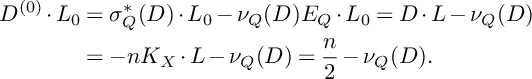 $$ \begin{align*} D^{(0)}\cdot L_0&=\sigma_Q^*(D)\cdot L_0 - \nu_Q(D)E_Q\cdot L_0=D\cdot L - \nu_Q(D)\\ &=-nK_X\cdot L - \nu_Q(D)=\frac{n}{2}-\nu_Q(D). \end{align*} $$
On the other hand, by Lemma 6.2 and $(iii)$
of Theorem 6.1,
$(iii)$
of Theorem 6.1,
 $$ \begin{align*} D^{(1)}\cdot L_1 = (\sigma_1^* D^{(0)} - \lambda_1 E^{(1)}) (\sigma_1^* L_0 + f_1) = D^{(0)} \cdot L_0 + \lambda_1. \end{align*} $$
By Theorem 6.1, we have $\sigma _i^*L_{i}=L_{i+1}$
for
$\sigma _i^*L_{i}=L_{i+1}$
for $i\geqslant 1$
. Thus, the equality
$i\geqslant 1$
. Thus, the equality $D^{(1)}\cdot L_{1}=D^{(i)}\cdot L_{i}$
holds for all
$D^{(1)}\cdot L_{1}=D^{(i)}\cdot L_{i}$
holds for all $i\geqslant 1$
.
$i\geqslant 1$
.
Denote $Z_i=D^{(i)}_1\cdot D^{(i)}_2$
, and we have the decomposition
$Z_i=D^{(i)}_1\cdot D^{(i)}_2$
, and we have the decomposition $Z_0=Z_v^{(0)}+Z_h^{(0)}+Z_Q$
, where
$Z_0=Z_v^{(0)}+Z_h^{(0)}+Z_Q$
, where $Z_Q \subset E_Q$
. We can disregard the part
$Z_Q \subset E_Q$
. We can disregard the part $Z_Q$
because it is away from P.
$Z_Q$
because it is away from P.
For every $Z_i$
, we have the part of the cycle in
$Z_i$
, we have the part of the cycle in $E^{(i)}$
, and let us denote it
$E^{(i)}$
, and let us denote it $\Gamma ^{(i)}$
. Recall that
$\Gamma ^{(i)}$
. Recall that $E^{(1)} \cong \mathbb {P}^1 \times \mathbb {P}^1$
and
$E^{(1)} \cong \mathbb {P}^1 \times \mathbb {P}^1$
and $E^{(i)} \cong \mathbb {F}_1$
for
$E^{(i)} \cong \mathbb {F}_1$
for $i\geqslant 2$
. The map
$i\geqslant 2$
. The map $\sigma _i \big \vert _{E^{(i)}}$
is the corresponding
$\sigma _i \big \vert _{E^{(i)}}$
is the corresponding $\mathbb {P}^1$
-fibration. We say that a curve B on
$\mathbb {P}^1$
-fibration. We say that a curve B on $E^{(i)}$
is vertical if
$E^{(i)}$
is vertical if $\sigma _i(B)$
is a point and horizontal otherwise. We can decompose the cycle
$\sigma _i(B)$
is a point and horizontal otherwise. We can decompose the cycle $\Gamma ^{(i)}$
into
$\Gamma ^{(i)}$
into $L_i$
with multiplicity, the rest of the horizontal part, and the vertical part:
$L_i$
with multiplicity, the rest of the horizontal part, and the vertical part:
 $$ \begin{align*}\Gamma^{(i)} = k_iL_i+C^{(i)}_h+C^{(i)}_v. \end{align*} $$
Since $E^{(i,i+h)}$
is disjoint from
$E^{(i,i+h)}$
is disjoint from $L_{i+h}$
for any
$L_{i+h}$
for any $h\geqslant 2$
,
$h\geqslant 2$
, $i\geqslant 2$
, we have
$i\geqslant 2$
, we have $\sigma ^* C^{(i,i+1)}\equiv C^{(i,i+h)}$
for any
$\sigma ^* C^{(i,i+1)}\equiv C^{(i,i+h)}$
for any $h\geqslant 2$
,
$h\geqslant 2$
, $i\geqslant 2$
. Similarly
$i\geqslant 2$
. Similarly $\Delta ^{(i)}\equiv \sigma ^* \Delta ^{(2)}$
for
$\Delta ^{(i)}\equiv \sigma ^* \Delta ^{(2)}$
for $i\geqslant 3$
since
$i\geqslant 3$
since $F^{(i)}$
is disjoint from
$F^{(i)}$
is disjoint from $L_i$
for
$L_i$
for $i \geqslant 2$
. Thus, we can decompose
$i \geqslant 2$
. Thus, we can decompose
 $$ \begin{align*} Z_0 &= Z_h^{(0)} + Z_v^{(0)} = Z_h^{(0)} + \Delta^{(0)} + k_0 L_0,\\ Z_1 &= Z_h^{(1)} + \Delta^{(1)} + C_h^{(1)} + C_v^{(1)} + k_1L_1,\\ Z_2 &= Z_h^{(2)} + \Delta^{(2)} + C_h^{(1,2)} + C_v^{(1,2)} + C_h^{(2)} + C_v^{(2)} + k_2L_2,\\ Z_i &= Z_h^{(i)} + \sigma^* \big( \Delta^{(2)} \big) + C_h^{(1,i)} + C_v^{(1,i)} + \sigma^*C_h^{(2,3)} + \sigma^*C_v^{(2,3)} \\ & \quad + \cdots \cdots + C_h^{(i-1,i)} + C_v^{(i-1,i)} + C_h^{(i)} + C_v^{(i)} + k_i L_i. \end{align*} $$
Recall that additional upper indices mean the proper transforms.
Denote the $\operatorname {mult}_{L_{i-1}}\mathcal {M}^{({i-1})}$
as
$\operatorname {mult}_{L_{i-1}}\mathcal {M}^{({i-1})}$
as $\lambda _i$
. Recall that by
$\lambda _i$
. Recall that by $f_i$
we denote the class of the fiber of the ruled surface
$f_i$
we denote the class of the fiber of the ruled surface $E^{(i)}$
. Thus,
$E^{(i)}$
. Thus, $C_v^{(i)} \equiv d_v^{(i)} f_i$
and
$C_v^{(i)} \equiv d_v^{(i)} f_i$
and $C_h^{(i)} \equiv d_h^{(i)} L_i + \beta _i f_i$
for some
$C_h^{(i)} \equiv d_h^{(i)} L_i + \beta _i f_i$
for some $d_v^{(i)}$
,
$d_v^{(i)}$
, $d_h^{(i)}$
, and
$d_h^{(i)}$
, and $\beta _i$
. Moreover,
$\beta _i$
. Moreover, $d_h^{(i)}\leqslant \beta _i$
, because
$d_h^{(i)}\leqslant \beta _i$
, because $C_h^{(i)}$
does not contain the exceptional section. Recall that
$C_h^{(i)}$
does not contain the exceptional section. Recall that $\delta = 1$
if
$\delta = 1$
if $L_1\subset F^{(1)}$
and
$L_1\subset F^{(1)}$
and $\delta = 0$
otherwise. We now describe how the classes in components of
$\delta = 0$
otherwise. We now describe how the classes in components of $Z_{i}$
change as we climb up the staircase.
$Z_{i}$
change as we climb up the staircase.
Lemma 7.6. We have the following relations for the proper transforms and the pullbacks of the cycles:
 $$ \begin{align*} &\Delta^{(1)} \equiv \sigma^*_1 \Delta^{(0)} - \big( \Delta^{(0)}\cdot L_0 \big)_{F^{(0)}} f_{1},\\ &\Delta^{(2)} \equiv \sigma^*_2 \Delta^{(1)} - \delta (\Delta^{(0)} \cdot L_0)_{F^{(0)}} f_{2},\\ &C_h^{(1,i+1)} \equiv \sigma^*_{i+1} C_h^{(1,i)} - \beta_1 f_{i+1} \quad \text{for} ~ i\geqslant 1,\\ &C_v^{(1,i+1)} \equiv \sigma^*_{i+1} C_h^{(1,i)} - d_v^{(1)} f_{i+1} \quad \text{for} ~ i\geqslant 1,\\ &C_h^{(i,i+1)} \equiv \sigma^*_{i+1} C_h^{(i)} - \big( \beta_i - d^{(i)}_h \big) f_{i+1} \quad \text{for} \quad i\geqslant 2,\\ &C_v^{(i,i+1)} \equiv \sigma^*_{i+1} C_v^{(i)} - d^{(i)}_v f_{i+1} \quad \text{for} \quad i\geqslant 1,\\ &Z_h^{(i+1)} \equiv \sigma^*_{i+1} Z_h^{(i)} - \alpha_{i+1} f_{i+1} \quad \text{for some} \quad \alpha_{i+1} \leqslant 2n^2. \end{align*} $$
Proof. First equivalence follows from Lemma 7.1 directly. If $\delta = 0$
, that is, if
$\delta = 0$
, that is, if $F^{(1)}$
and hence
$F^{(1)}$
and hence $\Delta ^{(1)}$
is disjoint from
$\Delta ^{(1)}$
is disjoint from $L_1$
, then we have
$L_1$
, then we have $\Delta ^{(2)} \equiv \sigma ^*_2 \Delta ^{(1)}$
. If
$\Delta ^{(2)} \equiv \sigma ^*_2 \Delta ^{(1)}$
. If $\delta = 1$
, that is, if
$\delta = 1$
, that is, if $L_1 \subset F^{(1)}$
, then the equivalence follows from Lemma 7.1.
$L_1 \subset F^{(1)}$
, then the equivalence follows from Lemma 7.1.
Note that
 $$ \begin{align*} &(C^{(1,i)}_h \cdot L_i)_{E^{(1,i)}} = (C^{(1)}\cdot L_1)_{E^{(1)}} = \beta_1,\\ &(C^{(1,i)}_v \cdot L_i)_{E^{(1,i)}} = (C^{(1)}\cdot L_1)_{E^{(1)}} = d_v^{(1)},\\ &(C_h^{(i)} \cdot L_i)_{E^{(i)}} = \beta_i - d^{(i)}_h,\\ &(C_v^{(i)} \cdot L_i)_{E^{(i)}} = d^{(i)}_v. \end{align*} $$
Thus, all equivalences but the last follow from Lemma 7.1. By Lemma 7.2, we have
 $$ \begin{align*}\alpha_i \leqslant Z_h^{(i)} \cdot E^{(i)} \leqslant Z_h \cdot F. \end{align*} $$
Let $D_1,D_2$
be general divisors in
$D_1,D_2$
be general divisors in $\mathcal {M}$
, then
$\mathcal {M}$
, then
 $$ \begin{align*}Z_h \cdot F = D_1 \cdot D_2 \cdot F = 2 n^2, \end{align*} $$
since $D_i \in \big | -n K_X + l n F \big |$
.
$D_i \in \big | -n K_X + l n F \big |$
.
Lemma 7.7. We have the following relations for vertical degrees on $X^{(i)}$
. For
$X^{(i)}$
. For $i=1$
,
$i=1$
,
 $$ \begin{align*} \beta_1 + d_v^{(1)} = \alpha_1 + \big( \Delta^{(0)} \cdot L_0 \big)_{F^{(0)}} - \lambda_1 \big( n - 2\nu_Q(D) \big) - 2\lambda_1^2 - k_1 - d_h^{(1)}, \end{align*} $$
for $i=2$
,
$i=2$
,
 $$ \begin{align*} \beta_2 + d_v^{(2)} = \alpha_2 + \delta \big( \Delta^{(0)} \cdot L_0 \big)_{F^{(0)}} - \lambda_1 \big( n - 2 \nu_Q(D) \big) - \lambda_2^2 - 2 \lambda_1 \lambda_2 + \beta_1 + d_v^{(1)}, \end{align*} $$
and for $i\geqslant 3$
,
$i\geqslant 3$
,
 $$ \begin{align*} \beta_i + d_v^{(i)} = \alpha_{i-1} + \big( \beta_1 + d_v^{(1)} \big) + d_v^{(i-1)} + \big( \beta_{i-1} - d_h^{(i-1)} \big) - \lambda_i \big( n - 2 \nu_Q(D) \big) - 2 \lambda_1 \lambda_i - \lambda_i^2, \end{align*} $$
where D is a general member in $\mathcal {M}$
.
$\mathcal {M}$
.
Proof. By Lemma 7.3, we have the equivalence
 $$ \begin{align*} Z_1 & \equiv \sigma^{*}(Z_0) + \lambda_1^2 \big( E^{(1)} \big)^2 - 2 \lambda_1 \big( D^{(0)} \cdot L_{0} \big) f_1 \\ & \equiv \sigma^{*} \big( Z_0 \big) - \lambda_1^2 \sigma^{*}(L_0) - \Big( \lambda_1 \big( n - 2 \nu_Q(D) \big) + 2 \lambda_1^2 \Big) f_1. \end{align*} $$
On the other hand, from the decomposition of $Z_1$
and Lemmas 6.4
$Z_1$
and Lemmas 6.4 $(i)$
and 7.6, we have
$(i)$
and 7.6, we have
 $$ \begin{align*} &Z_1 = Z_h^{(1)} + \Delta^{(1)} + C_h^{(1)} + C_v^{(1)} + k_1 L_1 \\ \equiv \sigma_1^* \big( &Z_h^{(0)} + \Delta^{(0)} + (k_1 + d_h^{(1)}) L_0 \big) + (\beta_1 + d_h^{(1)}) f_1 + C_v^{(1)} - \big( \alpha_1 + \big( \Delta^{(0)} \cdot L_0 \big)_{F^{(0)}} - k_1 \big)f_1. \end{align*} $$
Combining these equivalences, we conclude that, in $A^2(X^{(1)})/\sigma _1^* A^2(X^{(0)})$
, we have
$A^2(X^{(1)})/\sigma _1^* A^2(X^{(0)})$
, we have
 $$ \begin{align*} (\beta_1 + d_h^{(1)} + d_v^{(1)}) f_1 &\equiv C_h^{(1)} + C_v^{(1)} \\ &\equiv - \Big( \lambda_1 \big( n - 2 \nu_Q(D) \big) + 2 \lambda_1^2 \Big) f_1 + \big( \alpha_1 + \big( \Delta^{(0)} \cdot L_0 \big)_{F^{(0)}} - k_1 \big) f_1. \end{align*} $$
Similarly, by Lemma 7.3,
 $$ \begin{align*} &Z_2 \equiv \sigma^{*} \big( Z_1 \big) + \lambda_2^2 \big( E^{(2)} \big)^2 - 2 \lambda_2 \big( D^{(1)}_1 \cdot L_{1} \big) f_2 \\ &\equiv \sigma^{*} \big( Z_1 \big) - \lambda_2^2 \sigma^{*}(L_{1}) - \Big( \lambda_2 \big( n - 2 \nu_Q(D) \big) + \lambda_2^2 + 2 \lambda_1 \lambda_2 \Big) f_2. \end{align*} $$
From the decomposition of $Z_2$
and Lemma 7.7, we see that
$Z_2$
and Lemma 7.7, we see that
 $$ \begin{align*} Z_2 = Z_h^{(2)} + \Delta^{(2)} + C_h^{(1,2)} + C_v^{(1,2)} + C_h^{(2)} & + C_v^{(2)}+ k_2 L_2 \\ \equiv \sigma^* \big( Z_h^{(1)} + \Delta^{(1)} + C_h^{(1)} + C_v^{(1)} + k_2 L_{1} \big) & + C_h^{(2)} + C_v^{(2)}\\ - \big( \alpha_{2} + \delta \Delta^{(0)} & \cdot L_0 + \beta_{1} + d^{(1)}_v \big) f_2. \end{align*} $$
Combining these equalities, we conclude that, in $A^2(X^{(2)})/\sigma _1^* A^2(X^{(1)})$
, we have
$A^2(X^{(2)})/\sigma _1^* A^2(X^{(1)})$
, we have
 $$ \begin{align*} C_h^{(2)} + C_v^{(2)} \equiv (d^{(2)}_v + \beta_2)f_2 \equiv \big( \alpha_{2}& + \delta \big( \Delta^{(0)} \cdot L_0 \big)_{F^{(0)}} + \beta_1 + d_v^{(1)} \big) f_2\\ &- \Big( \lambda_2 \big( n - 2 \nu_Q(D) \big) + 2 \lambda_1 \lambda_2 + \lambda_2^2 \Big) f_2. \end{align*} $$
Hence, we find $d^{(2)}_v+\beta _2$
.
$d^{(2)}_v+\beta _2$
.
We treat the general case the same. Once again by Lemma 7.3, we have
 $$ \begin{align*} &Z_i \equiv \sigma^{*} \big( Z^{(i-1)} \big) + \lambda_i^2 \big( E^{(i)} \big)^2 - 2 \lambda_i \big( D^{(i-1)}_1 \cdot L_{i-1} \big) f \\ &\equiv \sigma^{*} \big( Z^{(i-1)} \big) - \lambda_i^2 \sigma^{*} (L_{i-1}) - \Big( \lambda_i \big( n - 2 \nu_Q(D) \big) + \lambda_i^2 + 2 \lambda_1 \lambda_i \Big) f_i. \end{align*} $$
Once again from the decomposition of $Z_i$
and Lemma 7.6, we see that
$Z_i$
and Lemma 7.6, we see that
 $$ \begin{align*} &Z_i \equiv Z_h^{(i)} + C_h^{(1,i)} + C_v^{(1,i)} + \sigma^* \big( \Delta^{(2)} + C_h^{(2,3)} + C_v^{(2,3)} + \dots + C_h^{(i-2,i-1)} + C_v^{(i-2,i-1)} \big) \\ & + C_h^{(i-1,i)} + C_v^{(i-1,i)} + C_h^{(i)} + C_v^{(i)} + k_i L_i = \sigma^* \big( Z_h^{(i-1)} + \Delta^{(1+\delta)} + C_h^{(1,i-1)} + C_v^{(1,i-1)} \\ &+ C_h^{(2,3)} + C_v^{(2,3)} + \dots + C_h^{(i-2,i-1)} + C_v^{(i-2,i-1)} + C_h^{(i-1)} + C_v^{(i-1)} + k_i L_{i-1} \big) + C_h^{(i)} + C_v^{(i)} \\ &- \big( \alpha_{i} + \beta_1 + d_v^{(1)} + (\beta_{i-1} - d^{(i-1)}_h) + d^{(i-1)}_v \big) f_i. \end{align*} $$
Combining these equalities, we conclude that, in $A^2(X^{(i)})/\sigma _1^* A^2(X^{(i-1)})$
, we have
$A^2(X^{(i)})/\sigma _1^* A^2(X^{(i-1)})$
, we have
 $$ \begin{align*} C^{(i)}_h + C^{(i)}_v \equiv \big( \alpha_{i-1} + \big( \Delta^{(0)} \cdot L_0 \big)_{F^{(0)}} + (\beta_{i-1} - d^{(i-1)}_h) + &d^{(i-1)}_v + \beta_1 + d_v^{(1)} \big) f_i \\ &- \Big( \lambda_i \big(n - 2 \nu_Q(D) \big) + 2 \lambda_1 \lambda_i + 2 \lambda_i^2 \Big)f_i. \end{align*} $$
Hence, we find $d^{(i)}_v+\beta _i$
.
$d^{(i)}_v+\beta _i$
.
Corollary 7.8. The vertical degrees are bounded as follows:
 $$ \begin{align*} &\beta_1 + d_v^{(1)} < 2 n^2 - 2 \lambda_1^2 + 4 n^2 \gamma,\\ &\beta_M + d_v^{(M)} < (M-1) \big( 2 n^2 - 2 \lambda_1^2 + 4 n^2 \gamma \big) + \sum_{i=2}^{M} \big( 2 n^2 - \lambda_i^2 - 2 \lambda_1 \lambda_i \big) + 4 \delta n^2 \gamma~~ \text{for}~ M \geqslant 2. \end{align*} $$
Proof. Since the pair $(X,\frac {1}{n}\mathcal {M})$
is canonical at Q, the inequality
$(X,\frac {1}{n}\mathcal {M})$
is canonical at Q, the inequality $n \geqslant 2 \nu _Q(D)$
holds. For
$n \geqslant 2 \nu _Q(D)$
holds. For $i=1$
, by Lemma 7.7, we have
$i=1$
, by Lemma 7.7, we have
 $$ \begin{align*} \beta_1 + d_v^{(1)} = \alpha_1 + \big( \Delta^{(0)} \cdot L_0 \big)_{F^{(0)}} - \lambda_1 ( n - 2 \nu_Q(D) ) - 2 \lambda_1^2 - k_1 - d_h^{(1)}. \end{align*} $$
Combining this with the inequalities $\alpha _1 \leqslant 2n^2$
,
$\alpha _1 \leqslant 2n^2$
, $k_1, d_h^{(1)} \geqslant 0$
, and
$k_1, d_h^{(1)} \geqslant 0$
, and $\big ( \Delta ^{(0)}\cdot L_0 \big )_{F^{(0)}} \leqslant \big (\Delta \cdot L\big )_F < 4 \gamma n^2$
, we get
$\big ( \Delta ^{(0)}\cdot L_0 \big )_{F^{(0)}} \leqslant \big (\Delta \cdot L\big )_F < 4 \gamma n^2$
, we get
 $$ \begin{align*} \beta_1 + d_v^{(1)} < 2 n^2 + 4 \gamma n^2 - 2 \lambda_1^2. \end{align*} $$
We prove the second bound by induction. Suppose $M=2$
. Then, using the same bounds, we get
$M=2$
. Then, using the same bounds, we get
 $$ \begin{align*} &\beta_2 + d_v^{(2)} = \alpha_{2} + \delta \big( \Delta^{(0)} \cdot L_0 \big)_{F^{(0)}} + d_v^{(1)} + \beta_{1} - \lambda_i ( n - 2 \nu_Q(D) ) - \lambda_1^2 - 2 \lambda_1 \lambda_2 \\ &< (2 n^2 + 4 \gamma n^2 - \lambda_1^2) + (2 n^2 - \lambda_2^2 - 2 \lambda_1\lambda_2) + 4 \delta \gamma n^2. \end{align*} $$
Now, suppose the inequality holds for $M-1$
. Then, similar to the previous case, we have
$M-1$
. Then, similar to the previous case, we have
 $$ \begin{align*} &\beta_i + d_v^{(i)} = \alpha_{i} + (\beta_1 + d_v^{(1)}) + d_v^{(i-1)} + (\beta_{i-1} - d_h^{(i-1)}) - \lambda_i ( n - 2 \nu_Q(D) ) - 2 \lambda_1 \lambda_i - \lambda_i^2 \\ &< ( 2 n^2 - 2 \lambda_1 \lambda_i - \lambda_i^2 ) + (\beta_1 + d_v^{(1)}) + d_v^{(i-1)} + \beta_{i-1}. \end{align*} $$
Combining this with the bound on $\beta _1 + d_v^{(1)}$
and the assumption of induction, we get the statement of the corollary.
$\beta _1 + d_v^{(1)}$
and the assumption of induction, we get the statement of the corollary.
Corollary 7.9. The following bounds on multiplicities hold.
-
(i) Let B be a fiber of a ruled surface
$E^{(i)}$
, then
$$ \begin{align*} \operatorname{mult}_B Z_1 =& \operatorname{mult}_B C^{(1)}_v \leqslant 2 n^2 - 2 \lambda_1^2 + 4 n^2 \gamma,\\ \operatorname{mult}_B Z_i =& \operatorname{mult}_B C^{(i)}_v \leqslant \sum_{i=2}^{M} \big( 4 n^2 - 2 \lambda_1^2 - \lambda_i^2 - 2 \lambda_1 \lambda_i \big) + 4 (M - 1 + \delta) n^2 \gamma, \quad \text{for} ~ i\geqslant 2. \end{align*} $$
-
(ii) Let B be a point on
$E^{(i)}$
, and suppose B is not on the exceptional section, then
$$ \begin{align*} &\operatorname{mult}_B (C^{(1)}_v + C^{(1)}_h) \leqslant \big( 2 n^2 - 2 \lambda_1^2 + 4n^2 \gamma \big),\\ &\operatorname{mult}_B (C^{(i)}_v + C^{(i)}_h) \leqslant \sum_{i=2}^{M} \big( 4 n^2 - 2 \lambda_1^2 - \lambda_i^2 - 2 \lambda_1 \lambda_i \big) + 4 (M - 1 + \delta) n^2 \gamma, \quad \text{for} ~ i\geqslant 2. \end{align*} $$


Proof. Clearly, $\operatorname {mult}_B C^{(i)}_v$
is bounded by a vertical degree
$\operatorname {mult}_B C^{(i)}_v$
is bounded by a vertical degree $d^{(i)}_v$
whether B is a point or a curve. Thus, the inequality holds if B is a curve.
$d^{(i)}_v$
whether B is a point or a curve. Thus, the inequality holds if B is a curve.
Similarly, if B is a point, then $\operatorname {mult}_B C^{(i)}_h\leqslant d^{(i)}_h$
, and hence
$\operatorname {mult}_B C^{(i)}_h\leqslant d^{(i)}_h$
, and hence $\operatorname {mult}_B (C^{(i)}_v + C^{(i)}_h) \leqslant d^{(i)}_v+d^{(i)}_h$
. Since
$\operatorname {mult}_B (C^{(i)}_v + C^{(i)}_h) \leqslant d^{(i)}_v+d^{(i)}_h$
. Since $C^{(i)}_h$
does not contain the exceptional section, we have
$C^{(i)}_h$
does not contain the exceptional section, we have $d^{(i)}_h\leqslant \beta _i$
. Therefore, by Corollary 7.8, the inequalities hold.
$d^{(i)}_h\leqslant \beta _i$
. Therefore, by Corollary 7.8, the inequalities hold.
8 Method of supermaximal singularity upstairs
In the previous section, we found an upper bound on the multiplicity of components of $Z_M$
at the center of
$Z_M$
at the center of $\nu $
on
$\nu $
on $X^{(M)}$
. In this section, we show that it contradicts Corti’s inequality.
$X^{(M)}$
. In this section, we show that it contradicts Corti’s inequality.
Lemma 8.1. The pair
 $$ \begin{align*} \bigg( X^{(M)}, \frac{1}{n} \mathcal{M}^{(M)} - \Big( \frac{1}{n}(n - \lambda_1 ) &+ \gamma \Big) E^{(1,M)} \\ -&\sum_{j=2}^M \Big( \frac{1}{n} \sum_{i=2}^{j} ( 2 n - \lambda_1 - \lambda_i) + (j - 1 + \delta) \gamma \Big) E^{(j,M)} - \gamma F^{(M)} \bigg) \end{align*} $$
is not canonical at $\nu $
on
$\nu $
on $X^{(M)}$
.
$X^{(M)}$
.
Proof. By Theorem 6.1, we have $L_i\subset E^{(1,i)}$
for all i and
$L_i\subset E^{(1,i)}$
for all i and $L_i \not \subset E^{(j,i)}$
for
$L_i \not \subset E^{(j,i)}$
for $i> j > 1$
, and therefore the following equivalence holds:
$i> j > 1$
, and therefore the following equivalence holds:
 $$ \begin{align*} K_{X^{(M)}} - E^{(1,M)} - \sum_{i=2}^{M} 2 (i - 1) E^{(i,M)} - \frac{1}{2} E_Q \sim \sigma^*(K_X). \end{align*} $$
We disregard $E_Q$
in this equivalence and in the next ones since
$E_Q$
in this equivalence and in the next ones since $E_Q$
is away from P. For a general member
$E_Q$
is away from P. For a general member $D\in \mathcal {M}$
, we have
$D\in \mathcal {M}$
, we have
 $$ \begin{align*} &D^{(1)} + \lambda_1 E^{(1)} \sim \sigma^*(D) \quad \text{and} \\ &D^{(M)} + \sum_{j=1}^M \Big( \sum_{i=2}^j (\lambda_i + \lambda_1) E^{(j,M)} \Big) \sim \sigma^*(D), \quad \text{for} ~ j\geqslant 2. \end{align*} $$
By Theorem 6.1 $(vii)$
and
$(vii)$
and $(viii)$
, we have
$(viii)$
, we have
 $$ \begin{align*} F^{(M)} + E^{(1,M)} + \sum_{j=2}^{M} ( j - 1 + \delta ) E^{(i,M)} = \sigma^*(F). \end{align*} $$
Thus, the pair in the statement of the lemma is the log pullback of the pair
 $$ \begin{align*} \Big( X, \frac{1}{n} \mathcal{M} - \gamma F \Big). \end{align*} $$
Hence, by Remark 2.6, the pair is not canonical at $\nu $
.
$\nu $
.
8.1 End of the proof of the Main Theorem
Suppose $X^{(M)}$
is as in Proposition 6.7, that is, the center of
$X^{(M)}$
is as in Proposition 6.7, that is, the center of $\nu $
on
$\nu $
on $X^{(M)}$
is not a point on the exceptional section of
$X^{(M)}$
is not a point on the exceptional section of $E^{(M)}$
. We consider the three possibilities for the center of
$E^{(M)}$
. We consider the three possibilities for the center of $\nu $
, and in each case, we obtain a contradiction.
$\nu $
, and in each case, we obtain a contradiction.
8.2 Case A
Suppose the center B of $\nu $
on
$\nu $
on $X^{(M)}$
is a fiber of the ruled surface
$X^{(M)}$
is a fiber of the ruled surface $E^{(M)}$
. Then the only divisor in the boundary which contains B is
$E^{(M)}$
. Then the only divisor in the boundary which contains B is $E^{(M)}$
. First, suppose
$E^{(M)}$
. First, suppose $M=1$
, then the pair
$M=1$
, then the pair
 $$ \begin{align*} \bigg( X^{(1)}, \frac{1}{n} \mathcal{M}^{(1)} - \Big( \frac{1}{n}(n - \lambda_1 ) + \gamma \Big) E^{(1)} \bigg) \end{align*} $$
is not canonical at $\nu $
. By Lemma 2.7,
$\nu $
. By Lemma 2.7,
 $$ \begin{align*} \operatorname{mult}_B Z_1> 4 n^2 - 4 n \lambda_1 + 4 n^2 \gamma. \end{align*} $$
Combining this inequality with Corollary 7.9, we get
 $$ \begin{align*} 2 n^2 - 2 \lambda_1^2 + 4 n^2 \gamma> 4 n^2 \frac{n - \lambda_1}{n} + 4 n^2 \gamma \end{align*} $$
or, equivalently,
 $$ \begin{align*} 0>2n^2-4n\lambda_1+2\lambda_1^2=2(n-\lambda_1)^2, \end{align*} $$
which is a contradiction.
Now, suppose $M \geqslant 2$
. By Lemma 8.1,
$M \geqslant 2$
. By Lemma 8.1,
 $$ \begin{align*} \Big( X^{(M)}, \frac{1}{n} \mathcal{M}^{(M)} - \Big( \frac{1}{n} \sum_{i=2}^{M} ( 2 n - \lambda_1 - \lambda_i) + (M - 1 + \delta) \gamma \Big) E^{(M)} \Big) \end{align*} $$
is not canonical at $\nu $
. By Lemma 2.7, we have
$\nu $
. By Lemma 2.7, we have
 $$ \begin{align*} \operatorname{mult}_B Z_M> \sum_{i=2}^M ( 8 n^2 - 4 n \lambda_1 - 4 n \lambda_i ) + 4 (M - 1 + \delta) n^2 \gamma. \end{align*} $$
Combining this inequality with Corollary 7.9, we get
 $$ \begin{align*} \sum_{i=2}^M (4 n^2 - 2 \lambda_1^2 - \lambda_i^2 &- 2 \lambda_1 \lambda_i) + 4 (M - 1 + \delta) n^2 \gamma \\ &> \sum_{i=2}^M ( 8 n^2 - 4 n \lambda_1 - 4 n \lambda_i ) + 4 (M - 1 + \delta) n^2 \gamma. \end{align*} $$
or, equivalently,
 $$ \begin{align*} (M - 1) \lambda_1^2 + \sum_{i=2}^M \big( 2 n - \lambda_1 - \lambda_i \big)^2 < 0, \end{align*} $$
which is again a contradiction.
8.3 Case B
Suppose the center B of $\nu $
on
$\nu $
on $X^{(M)}$
is a point which is not on
$X^{(M)}$
is a point which is not on $E^{(M-1,M)}$
. Then the only divisors in the boundary containing B are
$E^{(M-1,M)}$
. Then the only divisors in the boundary containing B are $E^{(M)}$
and possibly
$E^{(M)}$
and possibly $F^{(M)}$
if
$F^{(M)}$
if $M = 2$
.
$M = 2$
.
First, suppose $M = 2$
and
$M = 2$
and $B \in F^{(2)}$
, then
$B \in F^{(2)}$
, then $\delta = 1$
. Then the pair
$\delta = 1$
. Then the pair
 $$ \begin{align*} \bigg( X^{(2)}, \frac{1}{n} \mathcal{M}^{(2)} - \Big( \frac{1}{n}( 2 n - \lambda_1 - \lambda_2) + 2 \gamma \Big) E^{(2)} - \gamma F^{(2)} \bigg) \end{align*} $$
is not canonical at $\nu $
, and the components of
$\nu $
, and the components of $Z_2$
which may contain B are:
$Z_2$
which may contain B are: $Z_h^{(2)}$
,
$Z_h^{(2)}$
, $C_v^{(2)}$
,
$C_v^{(2)}$
, $C_h^{(2)}$
, and
$C_h^{(2)}$
, and $\Delta ^{(2)}$
. By Corti’s inequality, there are numbers
$\Delta ^{(2)}$
. By Corti’s inequality, there are numbers $0 < t, t_F \leqslant 1$
such that
$0 < t, t_F \leqslant 1$
such that
 $$ \begin{align*}& \operatorname{mult}_B Z_h^{(2)} + t \operatorname{mult}_B \big( C_v^{(2)} + C_h^{(2)} \big) + t_F \operatorname{mult}_B \Delta^{(2)} \\&\quad \geqslant 4 n^2 + t ( 8 n^2 - 4 n \lambda_1 - 4n \lambda_2 + 8 n^2 \gamma ) + 4 t_F n^2 \gamma. \end{align*} $$
On the other hand,
 $$ \begin{align*}\operatorname{mult}_B \Delta^{(2)} \leqslant \Delta^{(2)} \cdot E^{(2)} = \big( \Delta^{(0)} \cdot L_0 \big)_{F^{(0)}} \leqslant 4 n^2 \gamma, \end{align*} $$
and we already mentioned the bounds on the other cycles. Combining the bounds, we get
 $$ \begin{align*}2 n^2 + t ( 4 n^2 - 2 \lambda_1^2 - \lambda_2^2 - 2 \lambda_1 \lambda_2 + 8 n^2 \gamma ) + 4 t_F n^2 \gamma> 4 n^2 + t ( 8 n^2 - 4 n \lambda_1 + 8 n^2 \gamma ) + 4 t_F n^2 \gamma, \end{align*} $$
or, equivalently,
 $$ \begin{align*}2 n^2 + t \lambda_1 ^2 + t (2 n - \lambda_1 - \lambda_i)^2 < 0, \end{align*} $$
which is again a contradiction.
Note that the proper transform on $F^{(2)}$
of the half-line L which gave us so much trouble earlier is a part of
$F^{(2)}$
of the half-line L which gave us so much trouble earlier is a part of $C_h^{(2)}$
, and thus its contribution to multiplicity is bounded.
$C_h^{(2)}$
, and thus its contribution to multiplicity is bounded.
Suppose $M \geqslant 2$
and
$M \geqslant 2$
and $B \not \in F^{(2)}$
. Then the pair
$B \not \in F^{(2)}$
. Then the pair
 $$ \begin{align*} \bigg( X^{(M)}, \frac{1}{n} \mathcal{M}^{(M)} - \Big( \frac{1}{n} \sum_{i=2}^{M} ( 2 n - \lambda_1 - \lambda_i) + (M - 1 + \delta) \gamma \Big) E^{(M)} \bigg) \end{align*} $$
is not canonical at $\nu $
, and the components of
$\nu $
, and the components of $Z_M$
which may contain B are
$Z_M$
which may contain B are $Z_h^{(M)}$
,
$Z_h^{(M)}$
, $C_v^{(M)}$
, and
$C_v^{(M)}$
, and $C_h^{(M)}$
. By Corti’s inequality, there is a number
$C_h^{(M)}$
. By Corti’s inequality, there is a number $0 < t \leqslant 1$
such that
$0 < t \leqslant 1$
such that
 $$ \begin{align*}\operatorname{mult}_B Z_h^{(M)} + t \operatorname{mult}_B \big( C_v^{(M)} + C_h^{(M)} \big) \geqslant 4 n^2 + t \sum_{j=2}^M \big( 8 n^2 - 4 \lambda_1 n - 4 \lambda_i n \big) + 4 t (M - 1 + \delta) n^2 \gamma. \end{align*} $$
Combining this inequality with the bounds from Corollary 7.9, we get
 $$ \begin{align*} 2 n^2 + t \sum_{j=2}^M \big( 4 n^2 - 2 \lambda_1^2 &- \lambda_i^2 - 2 \lambda_1\lambda_i \big) + 4 t (M - 1 + \delta) n^2 \gamma \\ & > 4 n^2 + t \sum_{j=2}^M \big( 8 n^2 - 4 \lambda_1 n - 4 \lambda_i n \big) + 4 t (M - 1 + \delta) n^2 \gamma, \end{align*} $$
or, equivalently,
 $$ \begin{align*}2 n^2 + t (M-1) \lambda_1^2 + \sum_{i=2}^M (2 n - \lambda_1 - \lambda_i)^2 < 0, \end{align*} $$
contradiction.
8.4 Case C
Suppose the center B of $\nu $
on
$\nu $
on $X^{(M)}$
is a point on the intersection
$X^{(M)}$
is a point on the intersection $E^{(M)}\cap E^{(M-1,M)}$
. These are the only divisors of the boundary containing B, that is,
$E^{(M)}\cap E^{(M-1,M)}$
. These are the only divisors of the boundary containing B, that is, $B \not \in F^{(M)}$
. Denote
$B \not \in F^{(M)}$
. Denote $M^- = M - 1$
for compactness of formulae. The components of
$M^- = M - 1$
for compactness of formulae. The components of $Z_M$
which may contain B are:
$Z_M$
which may contain B are: $Z_h^{(M)}$
,
$Z_h^{(M)}$
, $C_v^{(1,M)}$
,
$C_v^{(1,M)}$
, $C_h^{(1,M)}$
,
$C_h^{(1,M)}$
, $C^{(M^-,M)}_h$
, and
$C^{(M^-,M)}_h$
, and $C^{(M^-,M)}_v$
. Furthermore, the pair
$C^{(M^-,M)}_v$
. Furthermore, the pair
 $$ \begin{align*} \bigg( X^{(M)}, \frac{1}{n} \mathcal{M}^{(M)} - \Big( \frac{1}{n} \sum_{i=2}^{M^-} ( 2 n - \lambda_1 - \lambda_i)& + (M^- - 1 + \delta) \gamma \Big) E^{(M^-,M)} \\ & - \Big( \frac{1}{n} \sum_{i=2}^{M} ( 2 n - \lambda_1 - \lambda_i) + (M - 1 + \delta) \gamma \Big) E^{(M)} \bigg) \end{align*} $$
is not canonical at $\nu $
. By Corti’s inequality, there are numbers
$\nu $
. By Corti’s inequality, there are numbers $0<t,t^-\leqslant 1$
such that
$0<t,t^-\leqslant 1$
such that
 $$ \begin{align*} \operatorname{mult}_B Z_h^{(M)} + t \operatorname{mult}_B \big( C_v^{(M)}& + C_h^{(M)} \big) + t_- \operatorname{mult}_B \big( C_v^{(M^-,M)} + C_h^{(M^-,M)} \big) \\ \geqslant 4 n^2 + t \sum_{j=2}^M \big( 8 n^2 - &4 \lambda_1 n - 4 \lambda_i n \big) + t^- \sum_{j=2}^{M^-} \big( 8 n^2 - 4 \lambda_1 n - 4 \lambda_i n \big) \\ &+ 4 t (M - 1 + \delta) n^2 \gamma + 4 t^- (M^- - 1 + \delta) n^2 \gamma. \end{align*} $$
By combining the inequality with the bounds from Corollary 7.9, we get
 $$ \begin{align*} 2 n^2 &+ t \sum_{j=2}^M \big( 4 n^2 - 2 \lambda_1^2 - \lambda_i^2 - 2 \lambda_1\lambda_i \big) + t^- \sum_{j=2}^{M^-} \big( 4 n^2 - 2 \lambda_1^2 - \lambda_i^2 - 2 \lambda_1\lambda_i \big) \\ & + 4 t (M - 1 + \delta) n^2 \gamma + 4 t^- (M^- - 1 + \delta) n^2 \gamma> \\ & > 4 n^2 + t \sum_{j=2}^M \big( 8 n^2 - 4 \lambda_1 n - 4 \lambda_i n \big) + t^- \sum_{j=2}^{M^-} \big( 8 n^2 - 4 \lambda_1 n - 4 \lambda_i n \big) \\ &\quad + 4 t (M - 1 + \delta) n^2 \gamma + 4 t^- (M^- - 1 + \delta) n^2 \gamma, \end{align*} $$
or, equivalently,
 $$ \begin{align*}2 n^2 + t (M - 1) \lambda_1^2 + t \sum_{i=2}^M (2 n - \lambda_1 - \lambda_i)^2 + t^- (M^- - 1) \lambda_1^2 + t^- \sum_{i=2}^{M^-} (2 n - \lambda_1 - \lambda_i)^2 < 0, \end{align*} $$
which is a contradiction.
In addition, this ends the process of exclusion of points in fibers containing singular points of X, and therefore the proof of the Main Theorem is complete. $\square $
Appendix. Explicit computations on
$K^2$
-condition

A.1 On preservation of the
$K^2$
-condition

Here, we prove a result in favor of $K^2$
-condition being preserved in the running of the Sarkisov links at singular points of X.
$K^2$
-condition being preserved in the running of the Sarkisov links at singular points of X.
Throughout this section, we assume that $\pi : X \to \mathbb {P}^1$
is a del Pezzo fibration and that X is a general quasi-smooth hypersurface of degree
$\pi : X \to \mathbb {P}^1$
is a del Pezzo fibration and that X is a general quasi-smooth hypersurface of degree $(4,\ell )$
in a
$(4,\ell )$
in a $\mathbb {P}(1,1,1,2)$
-bundle
$\mathbb {P}(1,1,1,2)$
-bundle $T = \mathbb {P}(1,1,1,2)_{(0,a,b,c)}$
. We may assume
$T = \mathbb {P}(1,1,1,2)_{(0,a,b,c)}$
. We may assume $0 \leqslant a \leqslant b$
without loss of generality, and allow c to take value in
$0 \leqslant a \leqslant b$
without loss of generality, and allow c to take value in $\mathbb {Z}$
. Let
$\mathbb {Z}$
. Let $u,v$
be the coordinates on the base
$u,v$
be the coordinates on the base $\mathbb {P}^1$
, and let
$\mathbb {P}^1$
, and let $x,y,z,w$
be the coordinates on the fiber.
$x,y,z,w$
be the coordinates on the fiber.
Denote by $M_T$
the divisor with the equation
$M_T$
the divisor with the equation $\{x = 0\}$
, and let
$\{x = 0\}$
, and let $M = M_T \big \vert _X$
. Denote by F a fiber of
$M = M_T \big \vert _X$
. Denote by F a fiber of $\pi $
on X, and let
$\pi $
on X, and let $F_T$
be a fiber of the
$F_T$
be a fiber of the $\mathbb {P}(1,1,1,2)$
-bundle. Thus, we have that
$\mathbb {P}(1,1,1,2)$
-bundle. Thus, we have that $X \sim 4 M_T + \ell F_T$
. Clearly, for the cone of effective divisors on the toric level, we have that
$X \sim 4 M_T + \ell F_T$
. Clearly, for the cone of effective divisors on the toric level, we have that
 $$\begin{align*}\begin{array}{ll} \operatorname{Eff}^1(T) = \langle M_T, F_T \rangle&\text{if } c\geq 0.\\ \end{array}\end{align*}$$
By the choice of T, we have $K_T = -5 M_T - (2 + a + b + c) F_T$
and by adjunction
$K_T = -5 M_T - (2 + a + b + c) F_T$
and by adjunction
 $$ \begin{align*}K_X = - M + (\ell - 2 - a - b - c) F.\end{align*} $$
The following relations for the intersection numbers are rather easy to calculate.
Lemma A.1. With notation as above, we have that
 $$ \begin{align*} & M_T^3 \cdot F_T = 1/2, \\ & 2 M_T^4 = - a - b - c/2,\\ & M^2 \cdot F = M_T^2 \cdot F_T \cdot X = 2,\\ & M^3 = M_T^3 \cdot X = \ell/2 - 2 a - 2 b - c. \end{align*} $$
Proof. The first equality is just computation on $\mathbb {P}(1,1,1,2)$
. The second equality follows from the fact that the intersection
$\mathbb {P}(1,1,1,2)$
. The second equality follows from the fact that the intersection $\{x=0\} \cap \{y=0\} \cap \{z=0\} \cap \{w=0\}$
is empty. The rest is computed by intersection with X.
$\{x=0\} \cap \{y=0\} \cap \{z=0\} \cap \{w=0\}$
is empty. The rest is computed by intersection with X.
Proposition A.2. Let $\pi \colon X \to \mathbb {P}^1$
be a del Pezzo fibration of degree
$\pi \colon X \to \mathbb {P}^1$
be a del Pezzo fibration of degree $2$
. Suppose X is a quasi-smooth hypersurface of bi-degree
$2$
. Suppose X is a quasi-smooth hypersurface of bi-degree $(4,\ell )$
in a
$(4,\ell )$
in a $\mathbb {P}(1,1,1,2)$
-bundle T over
$\mathbb {P}(1,1,1,2)$
-bundle T over $\mathbb {P}^1$
. Suppose
$\mathbb {P}^1$
. Suppose $c \geqslant 2b$
, then for any I, the variety
$c \geqslant 2b$
, then for any I, the variety $X_I$
is also a hypersurface in T of bi-degree
$X_I$
is also a hypersurface in T of bi-degree $(4,\ell )$
.
$(4,\ell )$
.
Proof. It is enough to prove the statement of the proposition for $X^\prime = X_{\{i\}}$
, then the general case follows for any I by induction.
$X^\prime = X_{\{i\}}$
, then the general case follows for any I by induction.
In §4.2, we represented $X^\prime $
as a complete intersection in
$X^\prime $
as a complete intersection in $V^\prime $
a
$V^\prime $
a $\mathbb {P}(1,1,1,2,2)$
-bundle over
$\mathbb {P}(1,1,1,2,2)$
-bundle over $\mathbb {P}^1$
. We change the coordinates in
$\mathbb {P}^1$
. We change the coordinates in $V^\prime $
to have a more convenient first equation.
$V^\prime $
to have a more convenient first equation.
Suppose the singularity for which we constructed a Sarkisov link is given by $x=y=z=u=0$
. Then we can decompose the coefficient at
$x=y=z=u=0$
. Then we can decompose the coefficient at $w^2$
in the following way:
$w^2$
in the following way:
 $$ \begin{align*}f(u,v) = u v^{N-1} + u^2 g(u,v). \end{align*} $$
The equations of $X^\prime $
in
$X^\prime $
in $V^\prime $
are
$V^\prime $
are
 $$ \begin{align*} u s = (v^{N-1} + u g(u,v)) w + q(x,y,z;u,v) \quad\text{and}\quad s w + r(x,y,z;u,v) = 0. \end{align*} $$
Let us change the coordinates $s = s_{\text {new}} + g(u,v) w$
. Then the new equations are
$s = s_{\text {new}} + g(u,v) w$
. Then the new equations are
 $$ \begin{align*} u s = v^{N-1} w + q(x,y,z;u,v) \quad\text{and}\quad s w + g(u,v) w^2 + r(x,y,z;u,v) = 0. \end{align*} $$
Since $c \geqslant 2b$
, we may also decompose
$c \geqslant 2b$
, we may also decompose
 $$ \begin{align*}q(x,y,z;u,v) = u q_1(x,y,z;u,v) + v^{N-1} q_2(x,y,z;u,v). \end{align*} $$
Indeed, the degree of the first equation is $(2,c+N)$
, and thus
$(2,c+N)$
, and thus
 $$ \begin{align*}q \in \langle u,v \rangle^{c+N-2b} \subset \langle u,v \rangle^N, \end{align*} $$
where $\langle u,v \rangle $
is the ideal generated by
$\langle u,v \rangle $
is the ideal generated by $u,v$
. Then we change coordinates
$u,v$
. Then we change coordinates
 $$ \begin{align*} &s = s_{\text{new}} + q_1(x,y,z;u,v),\\ &w = w_{\text{new}} - q_2(x,y,z;u,v). \end{align*} $$
The new first equation is $u s = v^{N-1} w$
. Clearly, this equation defines a
$u s = v^{N-1} w$
. Clearly, this equation defines a $\mathbb {P}(1,1,1,2)$
-bundle over
$\mathbb {P}(1,1,1,2)$
-bundle over $\mathbb {P}^1$
. Let
$\mathbb {P}^1$
. Let $(u_T,v_T,x_T,y_Y,z_T,w_T)$
be the coordinates on T. Consider a map from T into
$(u_T,v_T,x_T,y_Y,z_T,w_T)$
be the coordinates on T. Consider a map from T into $V^\prime $
defined as follows:
$V^\prime $
defined as follows:
 $$ \begin{align*} &u = u_T, \quad v = v_T, \quad x = x_T, \quad y = y_T, \quad z = z_T,\\ &w = u w_T, \quad s = v^{N-1} w_T. \end{align*} $$
It is easy to see that this map is well defined and gives an embedding of T into $V^\prime $
. The equation of T in
$V^\prime $
. The equation of T in $V^\prime $
is
$V^\prime $
is $u s = v^{N-1} w$
, that is, the first equation of
$u s = v^{N-1} w$
, that is, the first equation of $X^\prime $
. Thus, we have
$X^\prime $
. Thus, we have $X^\prime $
embedded into T, substituting coordinates of T into the second equation we conclude that the equation of
$X^\prime $
embedded into T, substituting coordinates of T into the second equation we conclude that the equation of $X^\prime $
has degree
$X^\prime $
has degree $(4,\ell )$
that is the same degree as that of the equation of X in T.
$(4,\ell )$
that is the same degree as that of the equation of X in T.
Remark A.3. Let X be as in Proposition A.2, and suppose X satisfies the $K^2$
-condition. Then all
$K^2$
-condition. Then all $X_I$
live in the same family of hypersurfaces by Proposition A.2. Yet, we cannot say whether
$X_I$
live in the same family of hypersurfaces by Proposition A.2. Yet, we cannot say whether $X_I$
also satisfies the
$X_I$
also satisfies the $K^2$
-condition.
$K^2$
-condition.
The general expectation is that $K^2$
-condition is an open property in the moduli. Given this, let U be an open subset in a given family for which the
$K^2$
-condition is an open property in the moduli. Given this, let U be an open subset in a given family for which the $K^2$
-condition is satisfied. Then, by Proposition A.2, X satisfies the total
$K^2$
-condition is satisfied. Then, by Proposition A.2, X satisfies the total $K^2$
-condition if and only if
$K^2$
-condition if and only if $X_I \in U$
for all
$X_I \in U$
for all $I \subset \{1,\dots ,N\}$
, which suggests that
$I \subset \{1,\dots ,N\}$
, which suggests that $K^2$
-total condition must also be open in moduli.
$K^2$
-total condition must also be open in moduli.
A.2 Sufficient conditions for
$K^2$
-total condition

Lemma A.4. Let $D_1, D_2, D_3$
be divisors on X. Fix
$D_1, D_2, D_3$
be divisors on X. Fix $I \subset \{1,\dots ,N\}$
, and let
$I \subset \{1,\dots ,N\}$
, and let $G_1, G_2, G_3$
be divisors on
$G_1, G_2, G_3$
be divisors on $X_I$
of the same bi-degrees. Then
$X_I$
of the same bi-degrees. Then $D_1 \cdot D_2 \cdot D_3 = G_1 \cdot G_2 \cdot G_3$
.
$D_1 \cdot D_2 \cdot D_3 = G_1 \cdot G_2 \cdot G_3$
.
Proof. It is enough to check it for the case of $\deg G_1 = \deg G_2 = (1,0)$
and
$\deg G_1 = \deg G_2 = (1,0)$
and $\deg G_3 = (1,0)$
or
$\deg G_3 = (1,0)$
or $\deg G_3 = (0,1)$
. We are going to compute the intersections on the ambient scroll
$\deg G_3 = (0,1)$
. We are going to compute the intersections on the ambient scroll $V_{\big | I \big |}$
. Let
$V_{\big | I \big |}$
. Let $M_{\big | I \big |}$
be the divisor given by
$M_{\big | I \big |}$
be the divisor given by $x=0$
, and let
$x=0$
, and let $F_{\big | I \big |}$
be a fiber of the projection onto
$F_{\big | I \big |}$
be a fiber of the projection onto $\mathbb {P}^1_{u,v}$
. Then, similar to Lemma A.1, we compute that
$\mathbb {P}^1_{u,v}$
. Then, similar to Lemma A.1, we compute that $M_{\big | I \big |}^4 \cdot F_{\big | I \big |} = 1/4$
and
$M_{\big | I \big |}^4 \cdot F_{\big | I \big |} = 1/4$
and $4 M_I^5 = - a - b - \ell /2$
. Now, suppose
$4 M_I^5 = - a - b - \ell /2$
. Now, suppose $\deg G_3 = (0,1)$
, then
$\deg G_3 = (0,1)$
, then
 $$ \begin{align*}G_1 \cdot G_2 \cdot G_3 = M_{\big| I \big|}^2 \cdot F_{\big| I \big|} \cdot (2,\ell-c) \cdot (4,\ell) = 2. \end{align*} $$
If instead $\deg G_3 = (1,0)$
, then
$\deg G_3 = (1,0)$
, then
 $$ \begin{align*}G_1 \cdot G_2 \cdot G_3 = M_{\big| I \big|}^3\cdot (2,\ell-c) \cdot (4,\ell) = \ell/2 - 2a - 2b - c. \end{align*} $$
These intersections coincide with the ones we computed on X in Lemma A.1
Lemma A.5. For $X_I$
for any I we have the following. Let
$X_I$
for any I we have the following. Let $M_I$
denote the divisor given by
$M_I$
denote the divisor given by $x=0$
, and let
$x=0$
, and let $F_I$
be a fiber of
$F_I$
be a fiber of $\pi _I$
. Then the divisor
$\pi _I$
. Then the divisor $M_I + b F_I$
is nef.
$M_I + b F_I$
is nef.
Proof. The base locus of $\big | M_I + b F_I \big |$
is contained in
$\big | M_I + b F_I \big |$
is contained in $\{x=y=z=0\}$
. On the other hand,
$\{x=y=z=0\}$
. On the other hand,
 $$ \begin{align*}\{x=y=z=0\} = \{ \prod_{i\in I} l_i = w = 0 \} \cup \{ \prod_{j\not\in I} l_j = s = 0 \} = \operatorname{Sing} X_I, \end{align*} $$
which is of cardinality N. Thus, the base locus of $\big | M_I + b F_I \big |$
is finite, and hence
$\big | M_I + b F_I \big |$
is finite, and hence $M_I + b F_I$
is nef.
$M_I + b F_I$
is nef.
Proof of Proposition 1.7
First, let us compute $K_{X_I}$
. By adjunction, we have
$K_{X_I}$
. By adjunction, we have
 $$ \begin{align*} \deg K_{X_I} = \deg K_{V_{\big| I \big|}} + (2,c+N) + &(4,2c+N) = \\ &=\Big(-1, 3c + 2N - 2 - a - b - \big( c + \big|I\big| \big) - (c + N - \big| I \big|) \Big). \end{align*} $$
Since $d = 2c + N$
, we have
$d = 2c + N$
, we have
 $$ \begin{align*}\deg K_{X_I} = (-1, \ell - 2 - a - b - c) = \deg K_X. \end{align*} $$
If the intersection of $K_{X_I}^2$
with a nef divisor is nonpositive, then
$K_{X_I}^2$
with a nef divisor is nonpositive, then $K_{X_I}^2$
is not in the interior of the Mori cone. By Lemma A.5, the divisor
$K_{X_I}^2$
is not in the interior of the Mori cone. By Lemma A.5, the divisor $D_I = M_I + b F_I$
is nef, and by Lemma A.4, the intersection of
$D_I = M_I + b F_I$
is nef, and by Lemma A.4, the intersection of $K_{X_I}^2$
with
$K_{X_I}^2$
with $D_I$
is the same on all models
$D_I$
is the same on all models $X_I$
, and thus it is enough to compute it on X.
$X_I$
, and thus it is enough to compute it on X.
We compute
 $$ \begin{align*} K_X^2 \cdot D = (-1, \ell - a - b - c - 2)^2 \cdot (1,b) &= M^3 + (4 + 2a + 2b + 2c - 2 \ell + b) F \cdot M^2 =\\ &= 8 + 2a + 4b + 3c - \frac{7}{2} \ell. \end{align*} $$
If this value is nonpositive, all $X_I$
satisfy the
$X_I$
satisfy the $K^2$
-condition. This finishes the proof.
$K^2$
-condition. This finishes the proof.
Proof of Corollary 1.8
By assumption, $c \geqslant 2b$
, and thus Proposition 1.7 and the bounds
$c \geqslant 2b$
, and thus Proposition 1.7 and the bounds $0\leqslant 4a \leqslant 4b \leqslant 2c \leqslant \ell $
imply that
$0\leqslant 4a \leqslant 4b \leqslant 2c \leqslant \ell $
imply that
 $$ \begin{align*} a \leqslant 4, \quad 2b\leqslant 4 + a, \quad \text{and}~2c\leqslant 4 + a + 2b. \end{align*} $$
Using these inequalities, we fill the table.
Acknowledgments
A substantial part of this work was carried out while Igor Krylov was at the Max Planck Institute for Mathematics in Bonn. We would like to thank that institute for great hospitality and stimulating research environment. We would also like to thank Dr. Okada Takuzo for useful communications and for pointing out some inaccuracies in an earlier version.


 Open access