Introduction
Single-molecule localization microscopy (SMLM) techniques are based on the localization of individual molecules in a series of images acquired over time. Well-known examples are photoactivated localization microscopy (PALM [Reference Betzig1,Reference Hess2]), stochastic optical reconstruction microscopy (STORM [Reference Rust3]) and direct STORM (dSTORM [Reference Heilemann4]), ground state depletion followed by individual molecule return (GSDIM [Reference Fölling5]), and points accumulation for imaging in nanoscale topography (PAINT [Reference Sharonov and Hochstrasser6]). These approaches generate images of sparse random distributions of fluorescent molecules, which can be individually distinguished and localized (Figure 1). A series of such images is statistically analyzed to generate a table of the fluorophore locations and intensities. A high-resolution image can be constructed by rendering each location from the table as a tiny spot in the corresponding location in the image.
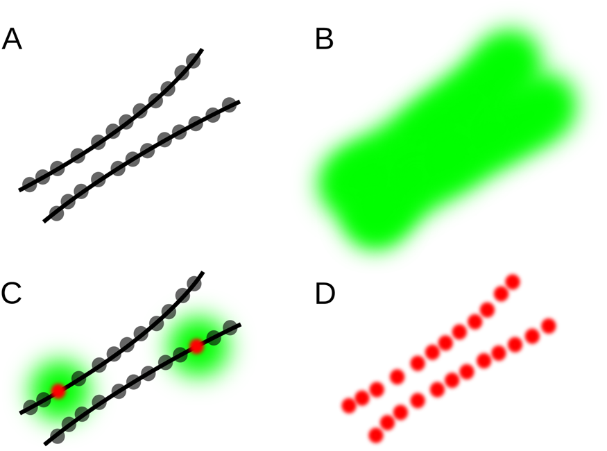
Figure 1: Principle of single-molecule localization microscopy (SMLM). (A) Example structure consisting of two closely spaced lines densely labeled with fluorophores (gray dots). (B) Because of light diffraction, the fluorescence of each fluorophore is detected as a spot in the shape of the microscope PSF, which add up to a single blurred shape where the lines cannot be resolved. (C) If only a few fluorophores are emitting, they can be localized with high precision (red dots), even though their PSF-sized image is relatively large (green). (D) By activating only a few fluorophores per image, and repeating this many times, all localizations can be determined with high precision, revealing the double-line structure.
Two-dimensional (2D) SMLM does not impose many demands on the optical system at the detection side and is usually implemented on a standard widefield or total internal reflection fluorescence (TIRF) microscope. The image of each fluorescent molecule is then given by the point spread function (PSF) of the microscope. 2D localization amounts to finding the position of the images of the molecules—in principle a straightforward task that does not critically depend on the shape of the PSF.
Three-dimensional (3D) SMLM is based on fitting the shape of the PSF. By introducing additional optical elements, such as a cylindrical lens, the shape of the PSF is made to vary strongly with the axial position. Hence, the shape of the PSF can be used to map the axial position of the fluorescent molecule. However, a calibration step that is complicated and error-prone is required and thus compromises reliable and accurate 3D SMLM analysis. To address this, we have adapted the Huygens PSF Distiller [7] so that an axial calibration map is easily calculated from microsphere images.
In addition to analysis tools shipped with the control software of commercial instruments, a wide selection of open-source options for localization microscopy is available [Reference Sage8,Reference Sage9]. However, the field seems to lack a generally applicable, well-supported, easy-to-use, high-performance package for 2D and 3D SMLM. This paper describes Huygens Localizer, the first commercially available standalone software package for SMLM, which aims to provide reliable, high-performance analysis and visualization of 2D and 3D SMLM data using a user-friendly workflow to interactively optimize the result. Here we present examples of the analysis of SMLM data with Huygens Localizer, including background detection, fitting, automatic drift correction, and visualization steps. We also describe 3D SMLM analysis, using the extended Huygens PSF Distiller to obtain an accurate PSF for calibration.
Materials and Methods
SMLM in 2D.
The principle of SMLM is explained in Figure 1. In short, the biological object is densely labeled with a fluorescent marker, for instance by immunofluorescence or by expressing fluorescent proteins. By exploiting the stochastic properties of a physical process, such as photo-activation (PALM [Reference Betzig1,Reference Hess2]), fluorophore blinking (STORM, dSTORM, GSDIM [Reference Rust3–Reference Fölling5]), or transient fluorophore binding (PAINT [Reference Sharonov and Hochstrasser6]), only a sparse random subset of the markers is active and visible at any given time. By imaging the sample at an appropriate rate, a time-series is obtained where each frame contains only the emissions of a small number of well-isolated fluorescent molecules, which show up as spots in the shape of the PSF of the microscope.
Given these sparse images, the lateral position of the molecules can be derived in a straightforward fashion: first the spots are isolated, and then their location is determined at sub-pixel resolution. The latter can be done by computing the center-of-mass of each spot. Alternatively and more accurately, the location can be obtained by fitting an analytical model of the PSF, often approximated by a 2D Gaussian function.
SMLM in 3D.
For 3D super-resolution imaging, the axial position of the molecules must also be derived with sub-diffraction precision. This is considerably more difficult since more information must be extracted from the noisy data. In standard wide-field detection, the distance of the fluorescent molecule to the focal plane can be derived from the size of the defocused PSF, but whether it is located above or below the focal plane is not easily determined. This problem can be overcome by generating an axially asymmetric PSF, such as an astigmatic PSF [Reference Huang10], or a double-helix PSF [Reference Pavani11], among others.
Here we focus on exploiting astigmatism, which is achieved by inserting a cylindrical lens into the detection path of the microscope. This leads to an elliptically shaped PSF, with a width-to-height ratio that depends on the distance and relative position to the focal plane, thereby uniquely encoding the axial position of the emitting molecule. To derive the 3D positions of the molecules in the data, a 2D elliptical Gaussian shape is fitted to each spot, determining its position, width, and height. The axial position can then be derived by comparing the width and the height to the values obtained using the PSF Distiller as outlined above.
Analysis of SMLM data.
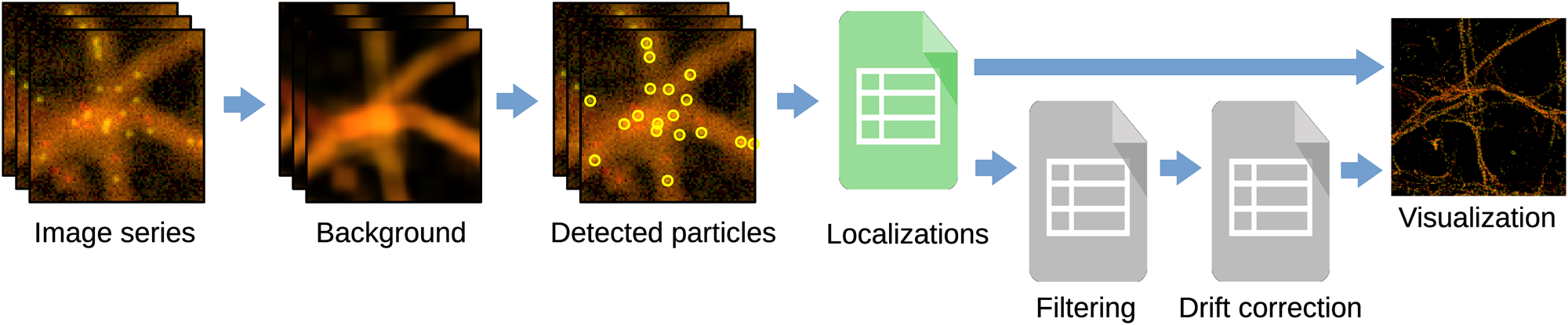
Figure 2 shows the steps followed by Huygens Localizer to turn a series of SMLM images into a table of localizations and a high-resolution image. The stages of the analysis pipeline include:
1. Background detection: Huygens Localizer implements a time-based background estimator that separates static structures from blinking fluorophores.
2. Detection of the single particles: The particles are detected in each frame by looking for local intensity maxima exceeding a threshold.
3. Localization of the detected particles: Each localization is fitted using maximum likelihood estimation, least-squares fitting, or center-of-mass determination. In 3D SMLM, the Z positions of the particles are also accurately calibrated.
4. Filtering of unwanted particles: Huygens Localizer implements several filters to interactively remove particles from the table of localizations.
5. Drift correction: Huygens Localizer offers an automatic drift corrector that does not require fiducial markers, avoiding the burden of introducing physical markers during sample preparation.
6. Visualization: Particles are rendered on the fly into a high-resolution image as single points or by placing small 2D/3D Gaussian spots at each particle location.

Figure 2: Huygens Localizer analysis pipeline. The first three steps form the core of the analysis pipeline, where the raw image series is transformed into a table of localizations. The steps to filter the localizations and correct for drift are optional. Finally, a super-resolved image is generated on-the-fly from the table of localizations.
In each of these steps Huygens Localizer leverages parallel computing on multi-core CPUs and GPUs in order to perform these calculations as quickly as possible. Importantly, this allows interactive adjustment of crucial parameters, such as the thresholds that affect particle detection.
Calibration of theZ position.
Calibration is generally done by imaging microspheres (∼100 nm) at small axial intervals (∼10 nm). The conventional approach to create calibration curves is to localize the microspheres and fit a 2D Gaussian shape at each Z position, followed by fitting defocusing curves to the resulting heights and widths [Reference Huang10]. Huygens Localizer improves on this approach by offering the option to fit a spline function for cases where the measured data deviate too much from a theoretical defocusing curve.
Besides fitting the microspheres directly, Huygens Localizer also offers the option to estimate the PSF using the Huygens PSF Distiller module. With the distiller module, an accurate, nearly noise-free PSF can be estimated from multiple microsphere images. The distilled PSF can then be used to calculate high-quality Z calibration curves that can be used instead of the noisier curves produced by the standard procedure. The result is a much more robust calibration procedure since an accurate and low-noise PSF is used as a basis for the calibration curves rather than noisy microsphere images.
Results
Accuracy, precision, and analysis speed.
Huygens Localizer uses state-of-the art statistical algorithms to achieve high accuracy (Figure 3A) and precision (Figure 3B) in comparison to the open-source package ThunderSTORM, as measured by the Jaccard index and the median distance to the true positions in simulations [12]. Even in the presence of high background levels, this level of high accuracy and precision is maintained, a feature that makes Huygens Localizer especially suited for biological applications where it is often difficult to prepare a “clean,” background-free sample. The Huygens Localizer algorithms are implemented with high performance on multi-core CPUs and are accelerated even more by offloading the calculations to massively parallel GPUs (Figure 4).
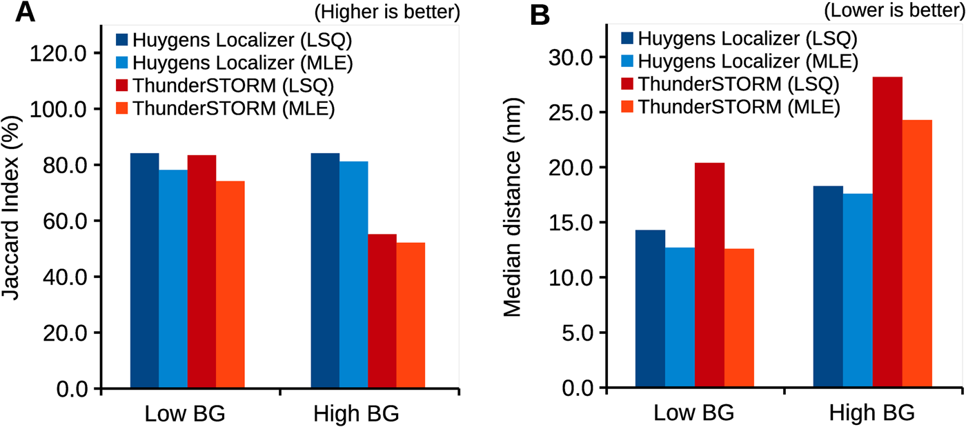
Figure 3: Accuracy and precision of Huygens Localizer, compared to the open-source package ThunderSTORM. Shown are results for simulated data that contain a low- and a high-static background, respectively. Both least squares (LSQ) fitting and maximum likelihood estimation (MLE) are tested. The results are based on realistic simulations of SMLM data, which are described in detail in the Huygens Localizer white paper that can be found on the Scientific Volume Imaging website: https://svi.nl/WhitePapers. (A) Plot of the Jaccard index, which summarizes the accuracy in terms of true positives, false positives, and false negatives. (B) Plot of the median distance between the estimated positions and the true positions of the simulated particles.
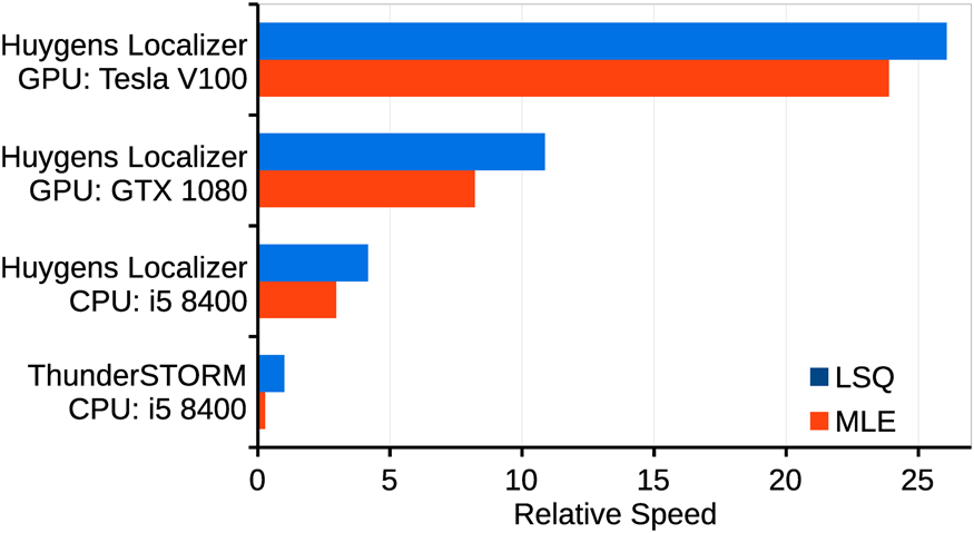
Figure 4: Comparison of the relative speed of Huygens Localizer with and without GPU acceleration, compared to the open-source package ThunderSTORM. Shown are the results for fitting with LSQ and for MLE. The results are normalized to the result for ThunderSTORM running a least-squares fit algorithm using an Intel i5 8400 CPU.
2D SMLM.
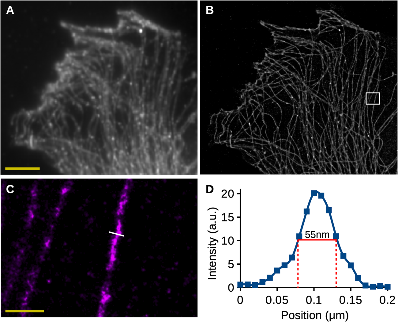
Figure 5 shows an example of the analysis of 2D SMLM images of a cell stained for tubulin. The data were acquired using a Nikon STORM system and analyzed using Huygens Localizer. Figure 5A shows a sum projection of the data over the time series corresponding to a standard widefield image. Figure 5B shows the visualization of the localization results, demonstrating a dramatically increased resolution, revealing the intricate structure of the microtubules.

Figure 5: Analysis of 2D SMLM data. (A) Sum projection of all images in the SMLM time-series, corresponding to a wide-field image. Scalebar: 5 µm. (B) High-resolution rendering of the SMLM localization results of Huygens Localizer. (C) High-resolution rendering of an area in (B) indicated by the white box. Scalebar: 0.5 µm. (D) A plot of the intensities along the line indicated in (C). The full width at half maximum is indicated in red and has a value of 55 nm.
To investigate the quality of the results obtained by Huygens Localizer in a biological sample, a profile of the intensities was drawn along a line perpendicular to a representative microtubule to measure its thickness (Figure 5C,5D). The full width of the microtubule at half its height was measured to be around 55 nm, which is in line with values reported earlier [Reference Wegel13], demonstrating the ability of Huygens Localizer to accurately recover biological structures from SMLM data of biological samples.
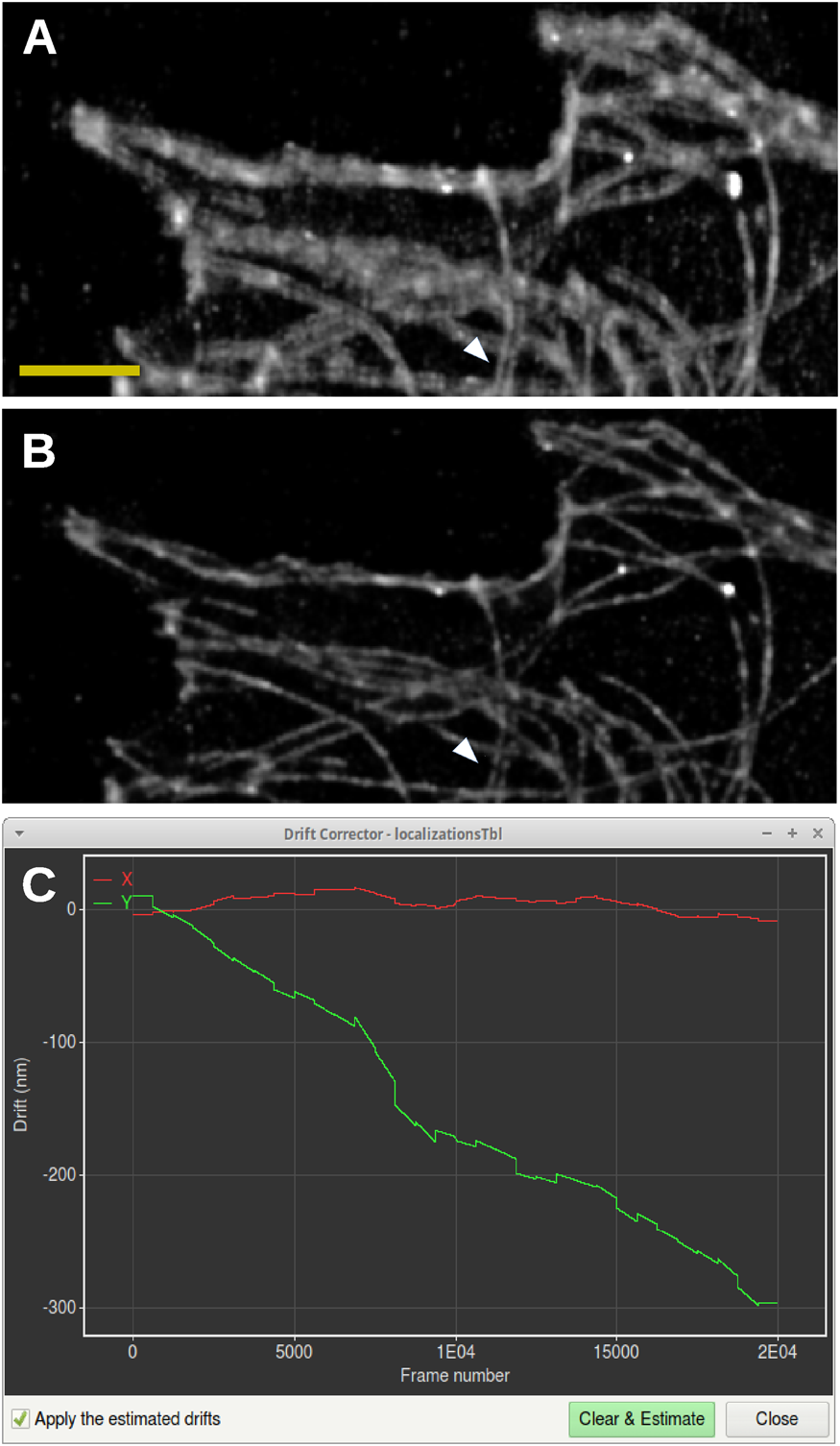
Without drift correction, a blurring of the data in the vertical direction can be observed, and many horizontally oriented microtubules appear as double lines (Figure 6A). After drift correction by Huygens Localizer, the vertical blurring has been removed, significantly sharpening the image, and the horizontal structures are revealed to be single lines (Figure 6B). Along the vertical direction only occasional double-line structures are observed (Figure 6A, white arrow), indicating that these are real structures, which are indeed preserved by the Huygens drift corrector (Figure 6B, white arrow). This is confirmed by a plot of the shifts showing a drift in the vertical direction of about 300 nm, but virtually no drift in the horizontal direction (Figure 6C).

Figure 6: Drift correction for SMLM data. (A) Rendering of SMLM localizations without correction for drift. Scale bar: 2 µm. (B) Rendering of SMLM localizations after corrections for drift using the Huygens Localizer drift corrector. The white arrows show a vertical double structure that is preserved by the drift corrector, in contrast to the horizontal double structures that are caused by drift. (C) Screenshot of the drift corrector, showing a plot of the shifts in the horizontal (red) and vertical (green) directions as a function of frame number in the time series.
3D SMLM.
Figures 7A–7D show four slices of an astigmatic PSF derived by the Huygens PSF Distiller from images of 100 nm Tetraspeck™ (Thermo Fisher Scientific) beads acquired by a Leica SR GSD system. The out-of-focus PSF has an ellipsoidal shape with an orientation depending on the relative position with respect to the focal plane. Far away from the focus (Figure 7D), the intensities of the PSF are spread out over a large area, which is harder to detect in the data, thereby limiting the axial range that is usable. Huygens Localizer fits a 2D Gaussian function to each PSF slice and generates high-quality calibration curves to relate the width and the height of the Gaussian to the Z position (Figure 7E).
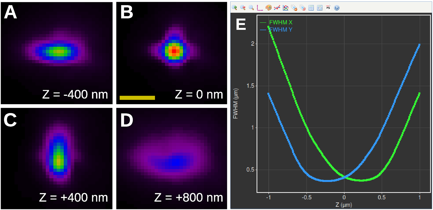
Figure 7: Measuring the PSF for 3D SMLM imaging. (A)–(D): PSF of an SMLM system equipped with a cylindrical lens as estimated by the Huygens PSF Distiller. Shown are four slices spaced 400 nm apart. Scale bar: 1 µm. (E): Screenshot of the PSF calibration curves derived and plotted by Huygens Localizer (blue curve: FWHM in the Y direction as a function of Z; green curve: FWHM in the X direction as a function of Z).
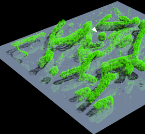
Figure 8 shows the results of a 3D SMLM analysis of DNA-PAINT images acquired with a Leica SR GSD system, using the Z calibration curves shown in Figure 7E. Human bone osteosarcoma epithelial (U2OS) cells were labeled with a primary antibody against the mitochondrial import receptor subunit TOM20 and with a secondary antibody conjugated with the DNA PAINT handle P1 [Reference Schnitzbauer14]. Imaging was performed with a 9 nt imager strand P1-Atto655 [Reference Schnitzbauer14]. Figure 8A shows a 3D representation created by the Huygens Simulated Fluorescence Process (SFP) renderer. The 3D structure of the mitochondria can be clearly discerned with most of the label residing on the outer membranes. This is shown clearly in the inset in figure 8A, which shows a high-resolution rendering of a globular structure (white arrow). The structure has been cut by a Z-plane through the middle, showing that it is hollow. Comparing a single slice from the middle of the 3D stack with the results of a 2D SMLM analysis highlights the accuracy of the 3D analysis by Huygens Localizer (Figure 8B,8C). In the 2D result it is impossible to judge the relative Z positions of the mitochondria, and it is not clear that only their outer membranes are labeled (Figure 8B). Yet, a single slice through the middle of the 3D result shows only mitochondria structures located at that depth, while the inner mitochondrial space is clearly not labeled (Figure 8C).
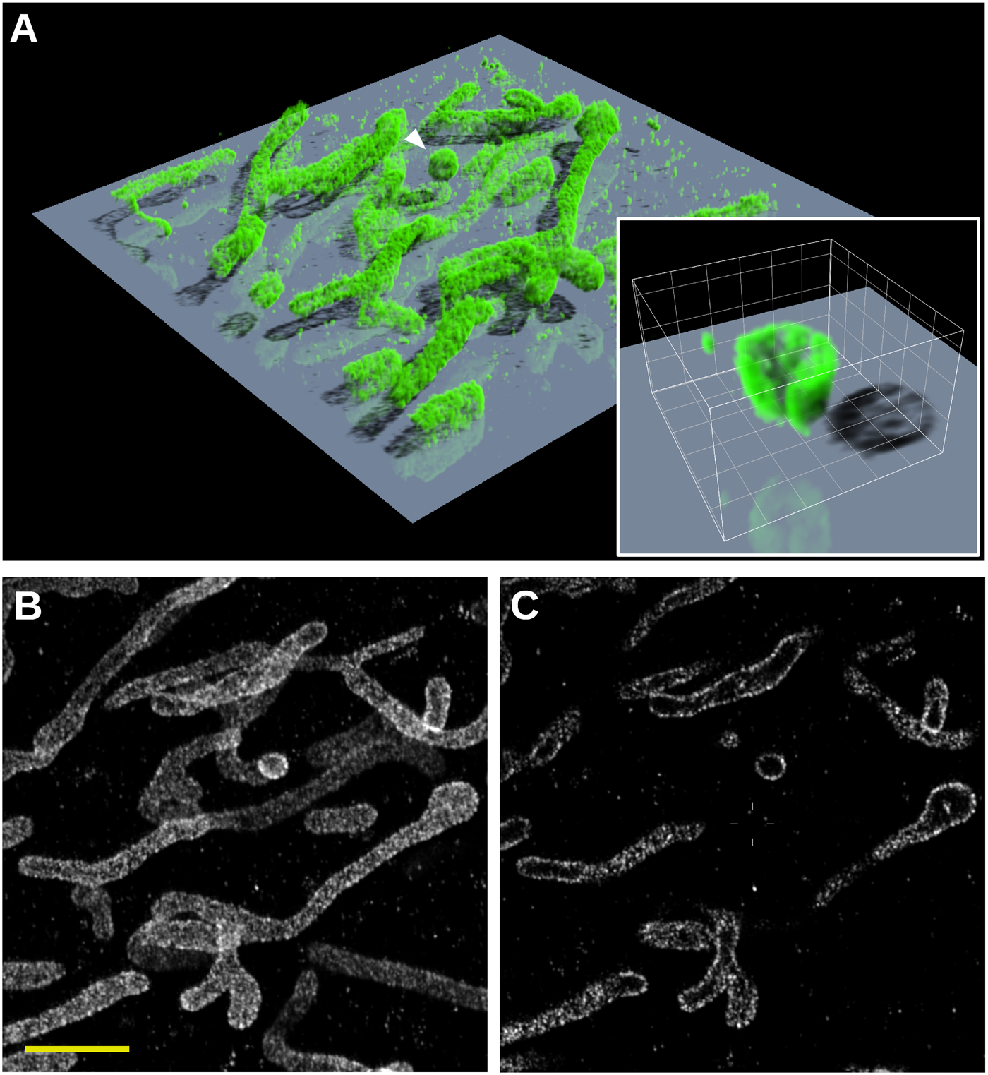
Figure 8: 3D SMLM analysis of the mitochondrial import receptor subunit TOM20 in human bone osteosarcoma epithelial (U2OS) cells using DNA-PAINT. (A) 3D SFP rendering of the 3D result. The size of the rendered volume is 10 µm × 10 µm × 1 µm. The inset shows a rendering of the globular structure indicated with the white arrow at a higher resolution, cut by a Z-plane through the middle of the structure. The step size of the shown grid is 200 nm. (B) Result of the 2D SMLM analysis of the data. (C) A single slice through the middle of the result of the 3D SMLM analysis showing effective depth discrimination of structures above or below the slice. Scalebar: 2 µm.
Discussion
SMLM techniques create images of biological objects in an indirect way, in contrast to most fluorescence microscopy techniques where the image is directly formed by imaging on a camera, or by scanning the sample. Instead, a time-series of sparse 2D images is acquired where the individual fluorophores can be distinguished. These data are processed to obtain a table of fluorophore locations together with a super-resolved image of the object. In the case of 3D SMLM, analysis is even more complicated due to the need to calibrate the Z position at a nanometer scale. Compared to direct imaging techniques, this imposes stricter requirements on the post-processing software, which must provide accurate localization results and visualizations, preferably at high speed.
Huygens Localizer fulfills these requirements by offering a user-friendly, wizard-driven interface to help with the complete SMLM data analysis pipeline, from background detection to rendering the super-resolved image. Using highly optimized multi-core CPU and GPU code, SMLM data can be analyzed and visualized quickly and accurately. Huygens Localizer includes the PSF Distiller, a time-tested module from the Huygens deconvolution package [7], which has been adapted to enable robust calibration of 3D SMLM data.
Several additional tools are included in Huygens Localizer. For example, results can be analyzed in more detail using the Huygens Object Analyzer module, which allows iso-surface-based quantitative measurements in the super-resolved images. The latest addition is the Huygens Batch Processor, which allows high-throughput analysis of SMLM data.
Conclusion
In this paper we presented Huygens Localizer for analyzing and visualizing SMLM data. Huygens Localizer provides researchers with a well-supported, easy-to-use, reliable, accurate, and very fast solution for the entire SMLM workflow. A demo version of Huygens Localizer can be downloaded from https://www.svi.nl/Download.
Acknowledgments
We thank Mikko Liljeström (Biomedicum Imaging Unit, University of Helsinki) for providing the data used in Figures 5 and 6. We thank Marko Lampe (Advanced Light Microscopy Facility, European Molecular Biology Laboratory, Heidelberg, Germany) for recording the data used in Figures 7 and 8 and Christoph Spahn and Mike Heilemann (Goethe University Frankfurt, Frankfurt am Main, Germany) for preparing the TOM20 DNA-PAINT sample. We thank Gert van Cappellen and Johan Slotman (Erasmus Medical Center, Rotterdam, the Netherlands) for helpful discussions and their great patience in evaluating early versions of the Huygens Localizer. We thank the LCI Resource Laboratory, University of Calgary, for their support and imaging advice.