


Introduction
Shape reconstruction methods via structured-light projection are used in the field of microscopic measurement. The structured light is projected onto the surface of a microscopic object by means of a special light source. The image of the structured-light pattern on the surface is acquired using computer vision methods. The three-dimensional (3D) positional data of the surface are generated by analyzing the structured-light image and developing a positioning algorithm. A 3D-morphology measurement method based on structured light has been applied in a variety of microscopic applications, such as wafer-surface reconstruction (Mei et al., Reference Mei, Gao, Lin, Chen, Yunbo, Wang, Zhang and Chen2016), ball-grid-array testing (Li et al., Reference Li, Liu and Tian2014; Li & Zhang, Reference Li and Zhang2015), and coin-surface reconstruction (Liu et al., Reference Liu, Chen, He, Thang and Kofidis2015). It is one of the noncontact optical measurement methods. Compared with the contact methods of microscopic measurement (e.g., scanning electron microscopes, atomic force microscopes, etc.), this method does not damage the sample surface and can be used to measure the attributes of living organisms, such as cells and microorganisms (Shao et al., Reference Shao, Kner, Rego and Gustafsson2011). Structured light techniques can be divided into many types. The phase analysis for sinusoidal fringe has been widely used (Liu & Su, Reference Liu and Su2014). It projects a fringe pattern of structured light with a sinusoidal distribution of light intensity onto the surface, and the stripe image and its phase were analyzed to obtain position data corresponding to the fringe pattern. Fringe-pattern scanning has also been commonly used. The structured light source is used to project a movable fringe onto the surface of the object, and then the fringe is adjusted to scan the entire surface. In this process, the images of the moving fringe were captured, and the sequence of the stripe images is constructed. Based on the analysis of this image sequence and the calculation of the triangulation principle, the 3D shape of the surface is generated. Speckle-based reconstruction has also been useful as a structured-light topography measurement method (De la Torre et al., Reference De la Torre, Montes, Flores-Moreno and Santoyo2016). It uses a special optical system to generate densely distributed spots and project them onto the surface of the object. Then, the speckle images were captured, and the surface topography data are generated by analyzing the shape and density distribution of the speckle. The above methods have different characteristics in reconstruction accuracy and flexibility. Sinusoidal fringe-patterned structured light has advantages in precision and accuracy through the hierarchical distribution and the phase-shifting technology of spatial brightness. Fringe-pattern scanning has more characteristics in flexibility and sensitivity while speckle structured light has a large spatial density and is more prominent in detail reconstruction.
The traditional structured-light projection system typically employs a laser light source and grating projection to generate a structured-light pattern. Using a line laser, it can directly project the striped structured light directly on the surface of an object. The line width of the striped structured light can be as narrow as tens of microns. Wang (Reference Wang2017) reconstructed the 3D morphology of some small objects (such as small resistors, gravel, and micro clamp tips) with a red line laser and binocular stereo vision system. The fine, monochromatic laser light source can generate high-intensity structured light. When a laser source irradiates an optical prism or other optical elements (De la Torre et al., Reference De la Torre, Montes, Flores-Moreno and Santoyo2016), speckle can be generated. The combination of a point light source and sinusoidal grating can produce fine sinusoidal fringes (Windecker & Tiziani, Reference Windecker and Tiziani1995). The fringes or the object can be adjusted to distribute the fringes across the surface of the object, and then the 3D shape of the object surface can be constructed by phase calculation. The point light source can be replaced by a bright halogen lamp or a laser. The incident beam is converted into a parallel beam through a collimating lens and then projected onto a sinusoidal grating. The outgoing beam passes through the microscope and projects onto the surface of the object to form the sinusoidal fringes. The structured-light pattern produced by laser light and sinusoidal grating cannot be too complex as its structure is relatively simple. Once the hardware is determined, the structure-light projection pattern is also fixed and cannot be changed. The method for solving spatial coordinates via structured light is also determined.
Universal projector devices have commonly been used in macroscopic scanning based on structured light (Gai et al., Reference Gai, Da and Dai2016; Guo et al., Reference Guo, Peng, Li, Liu and Yu2017), which employ 3D scanners to project structured-light patterns on the surface of objects. In the related research, digital micromirror devices (DMDs) and light-emitting diodes (LEDs) have been used in structured-light projection systems. DMD is a micromirror array, and the position of each micromirror can be adjusted by a control circuit. To reduce the overall volume, LEDs are often used for the light source. After the light beam irradiates the micromirror, the reflected light beam is filtered through a projection lens. The structured-light pattern may be speckle, thin fringes, or other patterns. Fukano & Miyawaki (Reference Fukano and Miyawaki2003) developed a DMD optical projection module to build a scanning system with fluorescence imaging for the inspection of biological samples. Zhang et al. (Reference Zhang, Van Der Weide and Oliver2010) also used a DMD optical projection module in their research to build a phase-shifted fringe-patterned projection system capable of achieving a scanning speed of 667 Hz. Dan et al. (Reference Dan, Lei, Yao, Wang, Winterhalder, Zumbusch, Qi, Xia, Yan, Yang, Gao, Ye and Zhao2013) designed a fringe-patterned projection system with DMD optical projection module and a low-coherence LED light. The longitudinal scanning depth of this system was 120 μm, and the horizontal resolution reached 90 nm. Chen et al. (Reference Chen, Shi, Liu, Tang and Liao2018) developed a system to project speckle patterns using a DMD module. They used a millimeter-scale cylinder array as a test sample to study the 3D measurement of a microstructure, which was nearly submicron. Most DMD projection modules have used an LED light source. The brightness of the structured light produced by an LED is relatively low, around 1,000 lumens, and the contrast is generally 1,000:1, which is more suitable for measuring the surface morphology of microscopic objects that have enhanced reflective intensity. However, for surfaces with weaker reflective intensity, structured light projected by an LED is not ideal. However, halogen projectors can overcome this issue with approximately 3,000 lumens and a contrast ratio of up to 10,000:1; in addition, they can generate arbitrary projection patterns via software. Moreover, the existing DMD projection modules do not support freely editing projection patterns and attributes.
The attributes of different types of microscopic objects can vary widely, and the requirements for measurement systems and processes were also varied. Some measurement environments require structured light with small size, high brightness, and high measurement accuracy, whereas other environments may need the opposite (e.g., large size and low brightness). For more comprehensive functionality, a structured-light projection system should be capable of generating various patterns according to the measurement requirements as well as have adjustable features (e.g., brightness, contrast, linewidth, etc.). Therefore, this study developed an adaptable structured-light projection system based on a conventional halogen lamp projector that would allow for manual customization of the projection pattern, including the color, line width, brightness, projection mode, etc. Using this system, the shape reconstructions of microscale objects were studied, and their surface morphology was described; then the calibration methods for the vision and projection systems were proposed. In addition, an algorithm for detecting the position of grid nodes in structured-light images was created.
The remainder of this article is organized as follows: In the section “Materials and Methods,” the materials and methods are described; in the section “Results and Discussion,” the experiment results and discussion were reported. In the section “Conclusion,” the conclusions were presented.
Materials and Methods
Design of the Structured-Light Projection System
The setup of the structured-light projection system developed in this paper is shown in Figure 1. Figure 1a presents the attributes of the structured-light pattern and the concept of attribute editing. The attributes of the structured-light pattern were edited using online software to adjust the pattern structure, color, geometric parameters (stripe length, width, etc.), position parameters, and motion parameters. The final design was projected onto the surface of the microscopic object via the projection system.
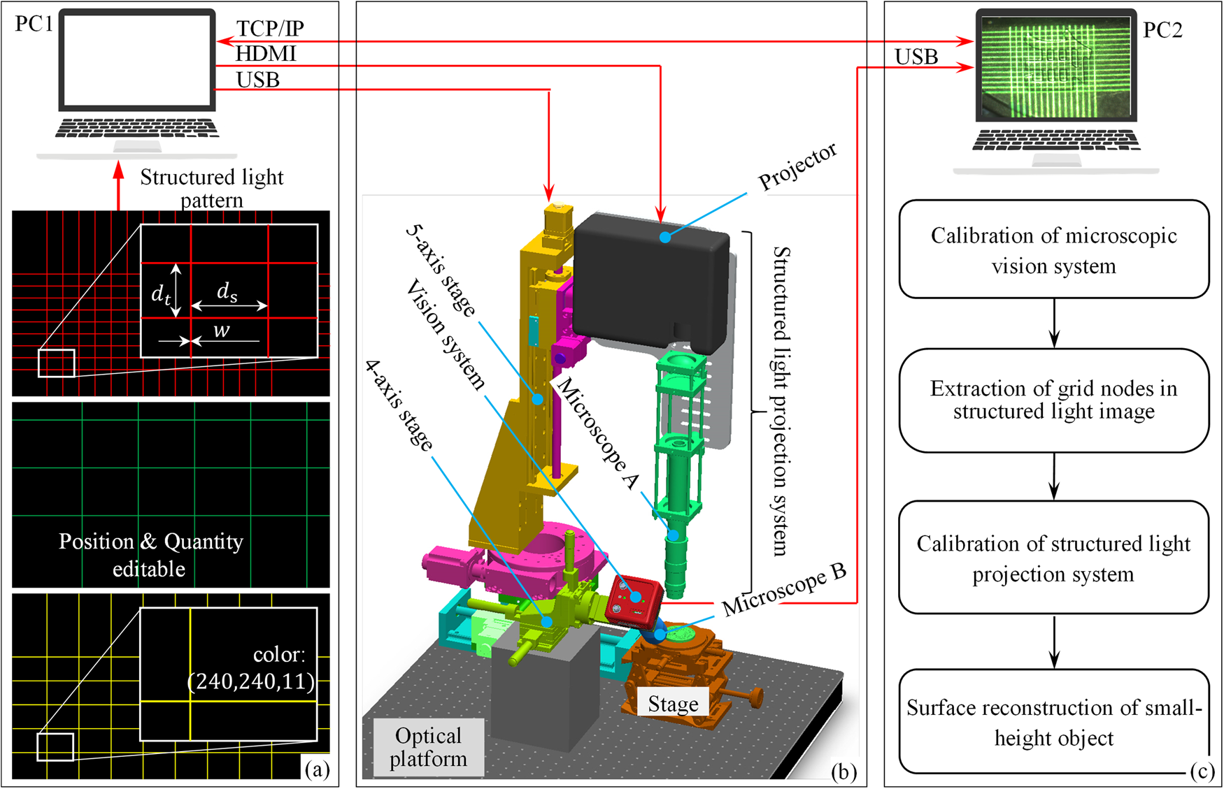
Fig. 1. Setup of the structured-light projection and measurement system. (a) Characteristics of projected structured light; (b) system setup; and (c) workflow of surface reconstruction.
Figure 1b shows the projection system for the structured-light pattern, consisting of a universal projector, an optical system with a tunable zoom lens, a carrier stage, a 5-axis position adjustment system for the projector, a 4-axis position adjustment system for the camera, an image acquisition system (including camera and microscope B), and computers (PC1 and PC2). The structured-light pattern was designed on PC1 and then sent to the projector to generate the beams. The small-scale structured-light pattern was transformed via the optical system with a tunable zoom lens (zoom range: 0.7×–4.5×) and projected onto the surface of the object. After the beams were reflected by the surface, it was imaged via microscope B and its integrated camera. The 5-axis position adjustment system was used to adjust the position and pose of the projector, so that the projector was coaxial with the optical system. It consisted of three translational and two rotational degrees of freedom. The repetitive precision positioning of horizontal and rotational degrees of freedom were 0.01 mm and 0.01°, respectively. The 4-axis position adjustment system was used to adjust the position and pose of the vision system, consisting of three translational and one rotational degrees of freedom, and their repetitive precision positioning were 0.01 mm and 0.01°, respectively. By adjusting the pitch angle of the camera, clear images of the structured-light pattern could be obtained, and the deformation of the structured-light pattern could also be adjusted. The stage could rise and fall vertically, which was also used to adjust the object so that the vision system could capture a clear image.
Figure 1c shows the technical method of surface reconstruction based on the structured-light projection system. It was divided into three modules: system calibration, grid-node detection, and graphic reconstruction. The calibration module was used to calibrate the camera and projector, estimate their position and distortion parameters, and improve the accuracy of the vision and projection systems. The grid-node detection module was used to obtain the coordinates of the grid nodes in the images, and these coordinates were then used as the parameters to calculate the world coordinates of the space nodes. The graphic reconstruction module was used to generate 3D representations of the surface on the computer.
The editing module for the structured-light pattern in Figure 1a expanded and refined the measurement range. We tested various surfaces of microscopic objects, and their reflection intensity of structured light were quite varied. By editing the attributes of the structured-light pattern, for example, the intensity, geometric size, color, pattern structure, and so on, it could be quickly adjusted according to the attributes of each object's surface. This significantly improved the success rate for different surface measurements. In addition, the system in Figure 1b used a universal projector, which was low cost and very convenient, and would adapt to more complex measuring instruments.
Reconstruction Method for Surface
In this paper, the 3D surfaces of short objects with diffuse reflections as a result of their metal surfaces were reconstructed. These objects were similar to microstructures with metal surfaces or metal structures with small dimensions in microelectromechanical systems (MEMS), such as 3D patterns on the surface of coins, gold-finger connectors, and metal-surface microstructures. They generally have small dimensions, especially in height. Structured light is critical to presenting height distribution. The height (or Z-direction) scale of microstructures may range from tens to hundreds of microns. However, the horizontal (X- or Y-direction) scales may be up to millimeters, as long as they are within the field of view of the microscope lens. The reflective abilities of these object surfaces vary widely and are based on their materials and attributes.
Figure 2 shows the flowchart of surface reconstruction of a microscale object. Firstly, the system was calibrated to determine the internal and external parameters of the vision and projection systems. The internal parameters of the vision system primarily included focal length, pixel size, and image distortion whereas the external parameters primarily included the translation and attitude angle between the camera coordinate system and the world coordinate system. The internal parameters of the projection system also include focal length, pixel size, and image distortion, whereas the external parameters were primarily rotation and translation between the coordinate systems. The system calibration process is shown in Figure 2a, which included establishing the mapping model between object and image points, obtaining the image and spatial coordinates of control points, analyzing image distortion, etc. The image and spatial coordinates of control points were provided by the plane calibration sample with a checkerboard pattern. In the sample, the lengths of cells were known, and their corner points were used as the control points for calibration. The coordinates of the control points were regarded as the world coordinates, and the image coordinates of the control points were generated by image preprocessing and corner-image-coordinate detection. The calibration of the projection system was different from that of the vision system. In the process of calibrating the projection system, it was necessary to project the grid pattern on a plane calibration sample. The nodes in the structured-light pattern were used as control points. The world coordinates of these nodes were provided by the calibrated vision system through calculation. The coordinates of the nodes in the structured-light pattern were known before projection. The mapping relationship between the projection surface and the world coordinate system were determined by using the spatial coordinates of the nodes and the coordinates in the projection pattern. The calibration of projection system also needed to establish a mapping model between object and image points as well as to correct the distortion on the projection plane.

Fig. 2. The workflow of system calibration and surface reconstruction. (a) The workflow of system calibration and (b) the workflow of surface reconstruction.
Figure 2b shows the process of surface reconstruction that primarily includes the following steps:
-
Step 1: The object was placed on the stage, the grid and structured-light pattern were projected onto the target surface, and the image was captured.
-
Step 2: The image was preprocessed, the image coordinates of the nodes in the grid were extracted, and the nodes in the image were aligned with the nodes in the projected grid pattern.
-
Step 3: The image coordinates of the node were input into the calibrated vision system, and then the world coordinates of the nodes were calculated, and the surface of the object was reconstructed based on the world coordinates of the nodes.
System Calibration
Calibration for the vision system
The measured objects in this paper were microscale objects. The horizontal scale range was typically from hundreds of microns to a few millimeters, and the vertical scale range was usually from tens to hundreds of microns. Therefore, the vision system (shown in Fig. 1) needed a magnification function. The microscope and camera were used together to build a microscope vision system with zoom capability, and the maximum magnification was 4.5×. A microscope vision system could perform the imaging processes required in this study from small to large. The size of the object (in the object space) was small, and the size of the image (in the image space) was large. In vision systems used for macroscale imaging, pinhole models are generally used to describe the mathematical mapping relationship between object and image points. We also used this model to construct the mapping relationship between object and image points in our microscope vision system.
Figure 3a describes the imaging and calibration principles of a pinhole model for a microscope vision system. Four coordinate systems were used to describe the relationships between object and image points, and they included a world coordinate system O-XYZ, a camera coordinate system O c-X cY cZ c, an image plane coordinate system o-xy, and image coordinate system q-uv. The first two are 3D coordinate systems, and the last two are 2D coordinate systems. In the process of calibration, the world coordinate system O-XYZ was usually placed in the plane calibration sample. The plane of the calibration sample was assigned as the plane O-XY, the Z-axis was perpendicular to the sample plane, and the origin O was located at a specific position on the sample plane. The origin O c of the camera coordinate system O c-X cY cZ c was set at the optical center of microscope B, the plane O c-X cY c was parallel to the image plane, and the Z-axis was perpendicular to the image plane and on the optical axis of microscope B. The origin o of the image plane coordinate system o-xy was located on the optical axis of microscope B, where |oO c| = f c, f c was the focal length in the image side. The plane xy was located on the imaging plane of microscope B, and the X- and Y-axes were parallel to the X c- and Y c-axes, respectively. The distance in the image plane coordinate system was measured in length units. The image coordinate system q-uv was placed in the image, and the origin q was located in the upper left corner of the image. The distance in the coordinate system q-uv was measured in pixel units, and the u- and v-axes were parallel to the x- and y-axes, respectively.
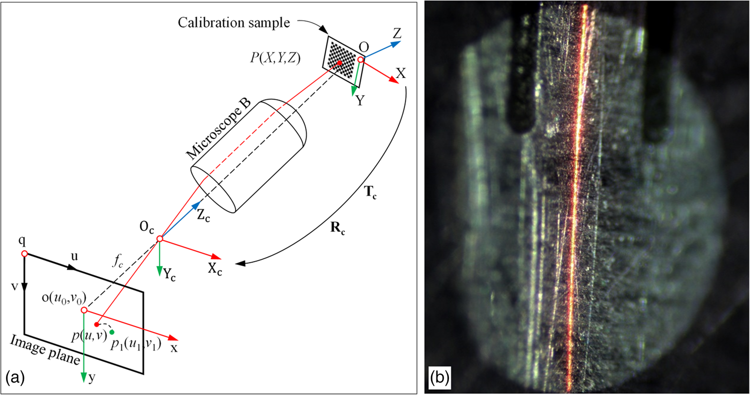
Fig. 3. Schematic diagram of vision system calibration. (a) Imaging description of vision system and (b) distortion of structured-light stripe in image.
The coordinates of the origin (o) in the coordinate system q-uv were represented by o(u 0,v 0), where u 0 and v 0 were measured in pixels. In addition, in the coordinate system q-uv, the length of a single pixel in x- and y-directions were expressed by dx and dy, respectively. A point P (X, Y, Z) in the coordinate system O-XYZ emitted light beams that passed through the optical center O c of microscope B; point P was imaged in the image coordinate system q-uv. If the image distortion was not considered, the image point was p(u,v). As can be seen from Figure 3a, once the values of dx, dy, u 0, v 0, and fc were determined, the internal structure of the vision system was also determined, and these parameters were considered the internal parameters. Relative rotation and translation relationships were identified between the coordinate systems O-XYZ and O c-X cY c. In Figure 3a, the rotation matrix and translation vector transformed from O-XYZ to O c-X cY cZ c are expressed by Rc and Tc, respectively, and the former is a 3 × 3 matrix, the latter is a 3 × 1 vector. Once Rc and Tc were determined, the relative position and attitude parameters of the vision system could be determined, and these parameters were considered the external parameters. According to the existing pinhole model, the mapping relationship between object point P(X,Y,Z) and image point p(u,v) is as follows:
 $$Z_u\cdot \left[{\matrix{ u \cr v \cr 1 \cr } } \right] = \left[{\matrix{ {\,f_x} & 0 & {u_0} & 0 \cr 0 & {\,f_y} & {v_0} & 0 \cr 0 & 0 & 1 & 0 \cr } } \right]\cdot \left[{\matrix{ {{\bf R}_{\bf c}} & {{{\bf T}}_{\bf c}} \cr 0 & 1 \cr } } \right]\cdot \left[{\matrix{ X \cr Y \cr Z \cr 1 \cr } } \right],$$
where fx = f c/dx, fy = f c/dy, fx, and fy represent the scale factors between the coordinate systems o-xy and q-uv, and Zu is a scale factor in the camera coordinate system Oc-XcYcZc.
Equation (1) is an ideal pinhole model without accounting for the image distortion, but image distortion is inevitable and will cause the real image point p 1(u 1,v 1) to deviate from the position of the ideal image point p(u,v). The ideal image point position had to be obtained by correcting the image distortion, and then it could be calculated by equation (1). Figure 3b shows an image of the red-fringe pattern captured by the vision system in Figure 1. In the case of no image distortion, the shape of the red fringe would be a straight line, but as can be seen from Figure 3b, the red fringe was bent, which indicated that there was distortion in the image. In this paper, radial and tangential distortions were considered. The correction formulas for these two kinds of distortion are as follows (De Villiers et al., Reference De Villiers, Leuschner and Geldenhuys2008):
 $$\matrix{ {\left\{{\matrix{ {u{\rm} = u_1( { 1 + k_ 1r_1^2 {\rm} + k_ 2r_1^4 } ) {\rm} + 2c_ 1u_1v_1{\rm} + c_ 2( r_1^2 {\rm} + 2u_1^2 ) }, \cr {v{\rm} = v_1( { 1 + k_ 1r_1^2 {\rm} + k_ 2r_1^4 } ) {\rm} + 2c_ 2u_1v_1{\rm} + c_ 1( r_1^2 {\rm} + 2v_1^2 ), } } } \right.} } $$
where k 1 and k 2 are radial distortion coefficients, c 1 and c 2 are tangential distortion coefficients, and  $r_1^2 = u_1^2 + v_1^2$. The calibration for the vision system is the process of estimating the above parameters. The Levenberg–Marquardt (LM) algorithm was used to optimize the objective function with all parameters (Hu et al., Reference Hu, Zhou, Cao and Huang2020a):
 $$\matrix{ {{\rm min}\left\{{\mathop \sum \limits_{i = 1}^n \mathop \sum \limits_{\,j = 1}^m \parallel {\bf u}_{{\bf a}, {\bf {ij}}}-{\bf u}_{{\bf c}, {\bf {ij}}}( {\,f_x, \;f_y, \;u_0, \;v_0, \;{\bf R}_{\bf c}, \;{\bf T}_{\bf c}, \;k_1, \;k_2, \;c_1, \;c_2} ) \parallel^2} \right\}} }, $$
where n is the number of images, m is the number of corner points in the calibration sample, ua,ij represents the real image coordinate vector of the j-th corner point in the i-th image, and uc,ij represents the image coordinate vector of the j-th corner point, as calculated by equations (1) and (2).
In the process of calibrating the vision system, a calibration sample with a checkerboard pattern of 13 lines × 12 columns was used to provide the world and image coordinates of control points. The size of calibration sample was 3.9 mm × 6 mm, the standard width of checkerboard cell was 0.3 mm, and the area of calibration sample accounted for about 60% of the field of view. The calibration process was divided into the following steps:
-
Step 1: The images of the calibration sample were captured at different positions in the field of view. The calibration sample was placed on the stage (as shown in Fig. 1), and then, the stage was adjusted to change the position of the calibration sample. A total of n positions were selected for placement, and n images were captured in the calibration process, where n was set to 15.
-
Step 2: The image coordinates of the corner point in the checkerboard were extracted. The images were preprocessed by a Gaussian filter, and the corner points in the images were detected by a region-growth method, and their image coordinates were obtained. These corner points were used as control points for calibration, and the number of control points was n × 12 × 11. The image coordinates of these control points constitute a set of {ua,ij} as true values of image coordinates.
-
Step 3: The world coordinates corresponding to the corner points in the images were obtained. The world coordinates of the corner points on the calibration sample were used as known quantities, and the data for calibration were generated by Steps 2 and 3.
-
Step 4: The world and image coordinates of the control points were used as the data for calibration, and the calibration of the vision system was calculated using equations (1)−(3), and the internal and external parameters were obtained.
Calibration for the projection system
In Figure 1b, the geometric size of the measured object was in microscale. A simple microscope was installed in front of the projector. Using the inverse-imaging principle of the microscope, the large projection pattern was transformed into a small pattern. Figure 4 depicts the calibration principle of the projection system. The projection system was regarded as a reverse-microscope vision system. The structured-light pattern was projected onto the sample surface through the projection system composed of projector, cage objective, and microscope A. Four coordinate systems were also used to describe the relationship between the object point and its image point in the structured-light pattern. These four coordinate systems included a world coordinate system O-XYZ, projector coordinate system O p-X pY pZ p, projection plane coordinate system a-bc, and projection image coordinate system w-st. The origin (O p) of the projector coordinate system O p-X pY pZ p was located at the optical center of the projector lens, the plane O p-X pY p was parallel to the DMD plane of the projector, and the Z p-axis was perpendicular to the DMD plane. The origin (a) of the projection plane coordinate system a-bc was located in the center of the DMD of the projector. The distance in the coordinate system was measured in length units. The b- and c-axes were parallel to the X p- and Y p-axes, respectively, where |aO p| = f p, and f p were the image focal length of the microscope A. The origin (w) of the projection image coordinate system w-st was located in the upper left corner of the projection image of the structured-light pattern. The distance in this coordinate system was measured in pixel units, and the s- and t-axes were parallel to the b- and c-axes, respectively.

Fig. 4. Schematic diagram of the projection system of structured light.
The coordinates of the origin (a) in the coordinate system w-st were represented by a(s 0, t 0), where s 0 and t 0 were measured in pixel units. In addition, in the coordinate system w-st, the length of a single pixel in s and t was expressed by ds and dt, respectively. A point P(X,Y,Z) in the coordinate system O-XYZ emits light beams. The beams pass through the optical center O p of microscope A, and was imaged in the image coordinate system w-st. If the image distortion was not considered, the image point was d(s,t). As can be seen from Figure 4a, once the values of ds,dt, s 0,t 0, and f p were determined, the internal structure of the projection system was also determined. Relative rotation and translation relationships were identified between the coordinate systems O-XYZ and O p-X pY p. In Figure 4a, the rotation matrix and translation vector transformed from O-XYZ to O p-X pY p were described by Rp and Tp, respectively, and the former was 3 × 3 matrix while the latter was 3 × 1 vector. Once Rp and Tp were determined, the relative position and attitude parameters of the projection system could be determined. According to the existing pinhole model, the mapping relationship between object point P(X,Y,Z) and image point d(s,t) is as follows:
 $$Z_v\cdot \left[{\matrix{ s \cr t \cr 1 \cr } } \right] = \left[{\matrix{ {\,f_b} & 0 & {s_0} & 0 \cr 0 & {\,f_c} & {t_0} & 0 \cr 0 & 0 & 1 & 0 \cr } } \right]\cdot \left[{\matrix{ {{\bf R}_{\bf p}} & {{\bf T}_{\bf p}} \cr 0 & 1 \cr } } \right]\cdot \left[{\matrix{ X \cr Y \cr Z \cr 1 } } \right],$$
where fb = f p/ds, fc = f p/dt, fb and fc represent the scale factors between the coordinate systems a-bc and w-st, and Zv is the scale factor in the coordinate system O p-X pY pZ p.
Since the projector system was regarded as a reverse-microscope vision system, similar to the image distortion processing in “Detection of Grid Nodes”, the distortion generated by the projection optical system should also be considered. In Figure 4a, the real image point d 1(s 1,t 1) deviated from the position of the ideal image point d(s,t). The position of ideal image point could be obtained by correcting the image distortion. In this paper, radial and tangential distortions were considered as follows:
 $$\matrix{ {\left\{{\matrix{ {s{\rm} = s_1( { 1 + k_3r_2^2 {\rm} + k_ 4r_2^4 } ) {\rm} + 2c_ 3s_1t_1{\rm} + c_ 4( r_2^2 {\rm} + 2s_1^2 ) }, \cr {t{\rm} = t_1( { 1 + k_ 3r_2^2 {\rm} + k_ 4r_2^4 } ) {\rm} + 2c_ 4s_1t_1{\rm} + c_ 3( r_2^2 {\rm} + 2t_1^2 ) }, } } \right.}} $$
where k 3 and k 4 are radial distortion coefficients, c 3 and c 4 are tangential distortion coefficients, and  $r_2^2 = s_1^2 + t_1^2$. Similarly, after the internal and external parameters were obtained according to the constraint conditions, they were taken as the initial values, and the maximum likelihood estimation method was used to optimize the parameters. LM optimization algorithm was used to optimize the objective function including all parameters:
 $$\matrix{ {{\rm min}\left\{{\mathop \sum \limits_{i = 1}^n \mathop \sum \limits_{\,j = 1}^m {\Vert { {{\bf s}_{{\bf a}, {\bf {ij}}}-{\bf s}_{{\bf c}, {\bf {ij}}}( {\,f_b, \;f_c, \;s_0, \;t_0, \;{\bf R}_{\bf p}, \;{\bf T}_{\bf p}, \;k_3, \;k_4, \;c_3, \;c_4} ) } \Vert } }^2} \right\},} } $$
where n is the number of images of the grid structured-light pattern, m is the number of node points, sa,ij represents the image coordinate vector of the j-th node point in the i-th image, and sc,ij represents the image coordinate vector of the j-th node point calculated by equations (4) and (5).
The calibration of projection system was divided into the following steps:
-
Step 1: Designing the projection image of the grid pattern of structured light in PC1, as shown in Figure 1. In the projection image, the image coordinates of the projection nodes in the grid pattern were known as the coordinates s and t.
-
Step 2: Projecting the image of the structured-light pattern through the projection system onto the surface of a flat calibration object (e.g., a calibration sample).
-
Step 3: Capturing the image of the structured-light pattern using the vision system. The image of the structured light was captured by PC2, as shown in Figure 1. The image coordinates of the node points (i.e., control nodes) were acquired using the image detection algorithm in the section “Detection of grid nodes.”
-
Step 4: The microscope vision system was calibrated so that, by importing the image coordinates of the control nodes, their corresponding coordinates in the world coordinate system O-XYZ could be calculated.
-
Step 5: The world coordinates of the control nodes and the image coordinates of the projection node were used as the data for calibration. After combining them with equations (4)–(6), they were used to calibrate the projection system and determine its internal and external parameters.
To ensure the accuracy of the calibration of the projection system, the position of the pattern in the projection image (the position of the structured light changes as it was projected onto the object space) was adjusted by the editing software. The structured-light pattern in the object space was distributed as evenly as possible in the field of view. A total of n projection positions were set, and n images of the structured-light pattern were acquired while these images were used for calibration, with n taken as 15.
Coordinate calculation
After the vision and projection systems had been calibrated, they were used to reconstruct the world coordinates of the points in object space. As shown in Figure 4, point d 1(s 1,t 1) in the projection image coordinate system was projected to the location of point P(X,Y,Z) in object space. The reflected light beam passed through the vision system and was imaged in the image coordinate system with image point p 1(u 1,v 1). In the process of reconstructing the coordinates of point P(X,Y,Z), the coordinates of points d 1(s 1,t 1) and p 1(u 1,v 1) were determined. Solving the system of equations by combining equations (1) and (4), the coordinates of point P(X,Y,Z) at d 1(s 1,t 1) and p 1(u 1,v 1) can be calculated from the coordinates of d 1(s 1,t 1) and p 1(u 1,v 1).
 $$\eqalign{\left[{\matrix{ X \cr Y \cr Z \cr 1} } \right] &= \left\{{\left[{\matrix{ {\,f_x} & 0 & {u_0} & 0 \cr 0 & {\,f_y} & {v_0} & 0 \cr 0 & 0 & 1 & 0 } } \right]\cdot \left[{\matrix{ {{\bf R}_{\bf c}} & {{\bf T}_{\bf c}} \cr 0 & 1 } } \right]}\right.\cr & -\left.\left[{\matrix{ {\,f_b} & 0 & {s_0} & 0 \cr 0 & {\,f_c} & {t_0} & 0 \cr 0 & 0 & 1 & 0 } } \right]\cdot \left[{\matrix{ {{\bf R}_{\bf p}} & {{\bf T}_{\bf p}} \cr 0 & 1 } } \right] \right\}^{{-}1}\left[{\matrix{ {Z_uu_1-Z_vs_1} \cr {Z_uv_1-Z_vt_1} \cr {Z_u-Z_v} \cr } } \right].}$$
Detection of Grid Nodes
In the reconstruction process depicted in Figure 2b, the image of the structured-light pattern was captured, and the image coordinates (u 1,v 1) of the grid node were obtained by the image algorithm. The world coordinates of the nodes were calculated after substitution with the image coordinates (s 1,t 1) of the projected node in equation (7). This section describes the algorithm for detecting the grid nodes in the image.
Microscopic images of structured light were captured by the microscope vision system. Due to the magnification of the microscope, the image properties such as sharpness and contrast of the image were significantly lower than those obtained by a single-camera vision system. In the section “Results and Discussion,” images of various types of structured light were captured using the microscope vision system, all of which had the above characteristics. As can be seen from the microscopic images taken in the section “Results and Discussion,” the grid lines were weakly visible, and their edges were not as sharp as the edges of the stripes in the macroscopic images. In addition, local areas in the image were easily affected by strong reflections and were more likely to cause bright spots. To account for the unique characteristics of microscopic images, the image-coordinate-extraction algorithm of grid nodes was designed, and its flow is shown in Figure 5. It contains the steps of image pre-processing, skeleton extraction of grid pattern, and detection of skeleton intersection points. The process of the algorithm was as follows:
-
Step 1: The image of structured light was preprocessed by Gaussian filtering algorithm. It adopted a 24-bit true-color bitmap format. Firstly, the average grayscale values of the three-color channels of the image were calculated and compared, and the grayscale image corresponding to the color channel with the highest average grayscale value was used to detect the nodes. Then, Otsu's method was used to calculate the binarization and closing operation of the single-color-channel image to generate the binarization image (image 1). The flow of this step is shown in Figure 5a.
-
Step 2: The skeletons of the grid lines were extracted based on image 1. A new image, image 2, was generated by first removing the burrs from image 1, then removing the isolated pixel points and filling the enclosed empty pixel points in turn. Then, image 2 was processed to refine the skeletons and obtain the grid lines with the line width of 1 pixel; then image 3 was generated. The subtraction operation was performed several times between image 3 and image 2. If the grayscale value of all pixels of image 3 was not 0, Step 2 was performed again, and then Step 3 would be performed if all were 0. The generation process of image 3 is shown in Figure 5b.
-
Step 3: The four templates M 1–M 4 were used to filter image 3, respectively, which were as follows:
 $$\eqalignno{M_1 & = \left[{\matrix{ 0 & 0 & 0 \cr 0 & 2 & {-1} \cr 0 & {-1} & 0 \cr } } \right], \;M_2 = \left[{\matrix{ 0 & 0 & 0 \cr {-1} & 2 & 0 \cr 0 & {-1} & 0 \cr } } \right], \;\cr M_3 &= \left[{\matrix{ 0 & {-1} & 0 \cr 0 & 2 & {-1} \cr 0 & 0 & 0 \cr } } \right], \;M_4 = \left[{\matrix{ 0 & {-1} & 0 \cr {-1} & 2 & 0 \cr 0 & 0 & 0 \cr } } \right].}$$


Fig. 5. Grid-extraction algorithm for the structured-light image. (a) The workflow of skeleton extraction of grid. (b) The workflow of extracting the 1-pixel-width grid lines. (c) The accurate intersection coordinates obtained through the optimization of the grid structure.
Image 3 was filtered to produce four new images. The corresponding pixels of these four new images were multiplied to constitute another image, which was then extracted from image 3 to obtain the image of the grid node. Finally, image 4 was generated by connecting the neighboring nodes through the expansion method. The flow of this step is shown in Figure 5c.
In Step 3, the width of the grid lines in image 3 was 1 pixel. The intersecting structure of the grid lines for grid skeletons could be classified into four types that are depicted in Figure 6a, with Г1, Г2, Г3, and Г4 representing the four types of intersecting grid lines. Г1 was a cruciform structure; Г2 and Г3 were staggered cruciform structures with misalignment in both horizontal and vertical directions. The difference between them was the presence or absence of overlap (Г2 was a nonoverlapping structure; Г3 was an overlapping structure). Г4 was a partially interlaced cross-type structure with misalignment only in the horizontal or vertical direction. Image 3 was filtered using templates M 1, M 2, M 3, and M 4 in turn to obtain four filtered images. The cruciform intersection structures in these images were transformed into the types shown in Figures 6b–6e. These four filtered images were multiplied, and a new image was synthesized. In the synthesized image, the intersecting structure of the grid lines was transformed into the type shown in Figure 6f. The synthesized image was compared to the original image 3 to obtain the nodes at the intersection of the grid lines. In the subtracted image, the structure of the intersection region is shown in Figure 6g. In Figure 6a, the cruciform of Г2 and Г4 was misaligned by a magnitude of 1–3 pixels. If the misalignment was large, it was possible that the pixels in the two regions of the intersection of Г2 and Г4 in Figure 6g would separate after the image operations described above. If the gravity center of the area block was used as the node of the grid line under such conditions, the position of the node may be misaligned. To resolve this problem, the corresponding binary image in Figure 6g was inflated. The pixels of the adjacent nodes were connected to obtain the results, as shown in Figure 6h. The gravity center of the connected region in Figure 6h was calculated so that the sub-pixel-level image coordinates of the nodes could be accurately obtained. The coordinates (u 1,v 1) of the nodes in equation (7) could be obtained using the above algorithm.

Fig. 6. Improvement of node-extraction algorithm by skeleton filtering. (a) Four intersecting structures of grid lines. (b–e) The intersecting structures of grid lines obtained by filtering using templates M 1–M 4. (f) The intersecting structures of grid lines obtained by filtering using templates multiplying calculation. (g) Node regions obtained by subtraction calculation between (f) and (a). (h) Node regions obtained by dilation.
For the grid nodes in the projected image, their parameters were determined by software, so that the geometry of the pattern and the position of the nodes were identified. The structured-light image was directly filtered using the templates M 1–M 4 to obtain an image containing only the grid nodes, with each node in the image being one pixel point. The images in Figure 7a were processed using the algorithm described above, resulting in image 1, image 3, and image 4, as shown in Figures 7b–7d. The projection pattern was processed using the same method. The results of the detection of the grid lines and their nodes are shown in Figures 7e and 7f.

Fig. 7. Process and results of grid-intersection extraction. (a) Captured grid image; (b) image 1; (c) image 3; (d) image 4; (e) projected grid image; and (f) the grid intersection points of the projection calculated by the above algorithm.
Results and Discussion
In this section, the precision of the image coordinate extraction for grid nodes, the error in the calibration, and the surface reconstruction were analyzed by experiments. The experiments were carried out using the system shown in Figure 1. The model of the projector was BenQ-MP625P with a maximum resolution of 1,024 × 768 pixels, and it had a high-pressure mercury-vapor lamp with a luminance of 2,700 lumens. The resolution of the camera was 4,000 × 3,000 pixels, and the size of a pixel in the sensor was 1.85 μm × 1.85 μm. The zoom range of microscope lens was 0.7×–4.5×, the variation range of the corresponding working distance was 89–96 mm, the range of view size was 6.0–1.0 mm, and the field of view (FOV) of the system was 3.9°–0.6°.
Experiments on the Image Coordinate Extraction of Grid Node
Observation of Structured-Light Projection
In this section, the projection performance was verified by observing the projection quality of structured-light patterns under differently colored lighting conditions. Three types of samples were used in this experiment: a flat frosted aluminum alloy surface, a Chinese coin, and a gold-finger connector. The grid patterns of red, green, and blue structured light were projected onto these samples, respectively. The images of the structured-light patterns were captured by the vision system, as shown in Figure 1b. Figure 8a shows the image of the flat frosted aluminum alloy sample. The red structured-light pattern was projected onto the surface of this sample, and the image of the red pattern is shown in Figure 8b. Figure 8c shows the results of the node detection for this type of sample. Figure 8d shows the image of gold-finger connector. A blue structured-light pattern was projected onto the surface, and the image of the blue pattern is shown in Figure 8e. Figure 8f shows the detection results of the nodes in the local image. Figure 8g shows the image of the Chinese coin. A green structured-light pattern was projected onto the surface, and the image of the green pattern is shown in Figure 8h. Figure 8i shows the detection results of the nodes in the local images of this type of sample.

Fig. 8. Results of node extraction. (a) Plane-calibration sample of frosted aluminum; (b) an image of the red grid structured light covering the surface of the calibration sample; (c) extracted node positions (green star marks) in the red grid image; (d) gold-finger connector sample on local memory sticks (copper surface spaced with epoxy resin); (e) an image of the blue grid structured light covering the surface of gold-finger connector; (f) extracted node positions (red star marks) in the blue grid image; (g) a character on the surface of a Chinese coin (brass); (h) an image of the green grid structured light covering the surface of the character; and (i) extracted node positions (blue star marks) in the green grid image.
As can be seen in Figures 8b, 8e, and 8h, the structured-light images were clear, but the width of the grid lines varied due to the different reflection coefficients of the different object surfaces. The width of the cells of the grid was approximately 0.23 mm, and the line width of the grid lines was approximately 0.02 mm. The above illustrated the ability to project a grid-like structured light for microscale objects using the system shown in Figure 1, which could generate structured light with different properties, depending on the object to be measured.
In Figure 8b, the red grid lines projected on the frosted aluminum alloy plane were, for the most part, distributed uniformly, and the width of the cells was relatively uniform, and no strong reflections or distortions were found. As shown in Figure 8c, the image coordinates of the grid nodes obtained were stable and uniformly arranged. In Figure 8h, the coin's reflectance was higher at certain locations on the surface due to the large arced bulge on the local surface and the high reflectance of the metal. The grayscale level of the grid points at these locations fluctuated considerably, which may have had an influence on the image coordinate extraction of the nodes. As shown in Figure 8i, there were small offsets and fluctuations in the positions of the nodes. To resolve this problem, the algorithm in the section “Detection of grid nodes” was improved. The pattern was projected to a background without any disruptions using the structured-light-projection software shown in Figure 1a. With this improved method, only background pixels existed in the projection pattern, with no grid lines or nodes. The grayscale values of the background pixels were set to g 1, g 2, and g 3; their values were smaller. The grayscale values of the red-, green-, and blue-color channels of the background pixels were set to g 1 = 40, g 2 = 40, and g 3 = 40. Then, the images of the structured-light pattern were processed according to the following steps to optimize the node-detection algorithm
-
Step 1: The background pattern was projected onto the surface of the object and its image was captured. The image of the background pattern was represented by S1.
-
Step 2: The grid pattern of structured light was projected onto the surface of the object and its image was captured. The image of the structured-light pattern was represented by S2.
-
Step 3: The images S1 and S2 were converted to grayscale images, and the grayscale images were represented by S11 and S21, respectively.
-
Step 4: The difference between S21 and S11 was calculated, and the extracted image S was obtained, where S = S21−S11.
-
Step 5: The skeletons of the grid pattern were extracted from the image S.
Figure 9 shows the results of the grid-skeleton extraction before and after the algorithm improvement. Figures 9a and 9b show the background image and the grid-pattern image, and Figure 9c shows the grayscale image from Figure 9b. Figure 9d shows the extracted image S obtained according to the improved algorithm. Figures 9e and 9f show the results of the grid-skeleton detection on the images in Figures 9c and 9d. As can be seen from Figure 9e, the mesh skeletons have localized misalignment, whereas the mesh skeletons in Figure 9d were more regularly arranged; therefore, the improved algorithm was effective.

Fig. 9. Treatments for highly reflective surfaces. (a) Image of the sample surface without structured-light pattern with background color (g 1,g 2,g 3) = (40,40,40); (b) image of the sample surface with structured-light pattern; (c) G-channel of b image; (d) G-channel of the image after a and b images have been differenced; (e) skeleton of the grid extracted by c image; and (f) skeleton of the grid extracted by d image.
Analysis of the Image Coordinate Extraction of Grid Node
A flat calibration sample of frosted aluminum alloy was chosen as the sample for the structured-light projection. The grid patterns of red, green, and blue structured light were projected onto the surface of the sample. The geometrical parameters of the structured-light pattern are shown in Figure 10a, with a line width of w = 1 pixel and a line spacing of ds = dt = 22 pixels in the s- and t-axis directions. After the pattern was projected into object space, the measured line width of the grid lines in the projected structured-light pattern was 0.02 mm, and the spacing was 0.24 mm. Figures 10b–10d present the red, green, and blue structured-light pattern images captured by the vision system. The image coordinates of the grid nodes were extracted using the algorithm described in the section “Detection of grid nodes,” and the following statistics were calculated based on the image coordinates: (1) The mean, minimum, maximum, and standard deviation of the distance du between adjacent nodes along the u-direction and (2) the mean, minimum, maximum, and standard deviation of the distance dv between adjacent nodes along the v-direction. The above parameters were used to evaluate the relative volatility of the grid-node position in the captured image, and the relative-volatility index reflected the accuracy of the grid-node coordinate extraction, to a certain extent.

Fig. 10. Principle of experiments to evaluate the accuracy of grid-node extraction. (a) Parameters of the projected grid; (b) statistical parameters in the red grid image; (c) statistical parameters in the green grid image; and (d) statistical parameters in the blue grid image.
The calculation results of the spacing parameters du and dv for each node in the red, green, and blue structured-light images are shown in Figures 11a and 11b. The values of du were distributed in the range of 26–31 pixels with a fluctuation interval of ±2.5 pixels, and the values of dv were distributed in the range of 24–30 pixels with a fluctuation interval of ±3.0 pixels. The values shown in Figure 11 were counted, and the results are shown in Table 1. As can be seen from Table 1, the mean values of du and dv in the red, green, and blue structured-light images were 28.5 and 26.7 pixels, respectively, with a standard deviation of less than 1 pixel. In addition, the statistical results showed that the average values of du and dv of the nodes in the red structured-light image were the largest, the average values of du and dv in the blue structured-light image were the smallest, and the average values of du and dv in the green structured-light image were in the middle, which indicated that the refractive indices of the samples for different colors of structured light were different, a result of the displacement offset of the nodes at the corresponding positions in different color images.

Fig. 11. The calculation results of du and dv correspond to (a) and (b), respectively.
Table 1. Statistical Results of du and dv.

Std, Standard deviation.
Analysis of the System Calibration Precision
In this section, the precision of the system calibration was analyzed by experiment. The reprojection error was frequently used for analyzing the error of the calibration for the vision and projection systems. The true values of the image and world coordinates of the test points were assumed to be (xa,ya) and (Xa,Ya,Za), respectively. The world coordinates of the test points were input into the calibrated system, and the image coordinates (xm,ym) of the test points were calculated as measured values. The reprojection error of the test points were defined in the following way.
 $$e = \sqrt {{( {x_m-x_a} ) }^2 + {( {y_m-y_a} ) }^2} .$$
To describe the distribution of the reprojection error more conveniently, the polar coordinate system was used in this study. In the polar coordinate system, e is used as the polar diameter, and the polar angle θ is given by the following formula:
 $${\rm tan}\theta = ( {y_m-y_a} ) /( {x_m-x_a} ). $$
In the experiment, the vision and the projection systems were calibrated individually, using the acquisition scheme for control points described in the section “System calibration.” The results of the internal and external parameters obtained by calibration are listed in Table 2.
Table 2. Parameters Obtained by System Calibration.

Figure 12a shows the results of the corner-point reprojection in one of the calibration sample images. Figure 12b shows the results for the node reprojection in one of the grid-pattern images. It can be seen from Figures 12a and 12b that the true and reprojection positions of the test points matched. The real positions of the test points coincided with their reprojection positions.

Fig. 12. Reprojection error. (a) Results of corner detection for checkerboard-type calibration sample where the red mark (“+”) represents the detected corners by algorithm, and the green mark (“o”) represents the calculated position by reprojection calculation. (b) The structured-light pattern obtained by reprojection calculation where the green mark (“o”) represents the calculated node position. (c) Distribution of reprojection error in 15 images of checkerboard-type calibration sample. (d) Distribution of reprojection error in 15 structured-light patterns.
The reprojection error was calculated according to equation (8), and the polar angle was calculated according to equation (9). Fifteen images with a total of 1,980 corner points were used, and the distribution of the reprojection error for these corner points is shown in Figure 12c. Figure 12c shows that the values of the reprojection error for the calibrated vision system were less than 0.5 pixels. Similarly, the reprojection error for the calibration projection system was calculated. Fifteen images with a total of 2,700 nodes were used, and the distribution of the reprojection error for these nodes is shown in Figure 12d. Figure 12d shows that the values of the reprojection error for the calibrated projection system were less than 0.8 pixels. The mean value, minimum value, maximum value, and standard deviation of the two types of reprojection errors related to Figures 12c and 12d were calculated. The results are listed in Table 3. As can be seen in Table 3, the reprojection error of the projection system was higher than that of the vision system, and its volatility was greater as well, which was related to the calibration process of the projection system. Because a calibrated vision system was utilized to provide the world coordinates of the control points required when calibrating the projection system, and the calibration error of the vision system had been inherited by the calibrated projection system. This resulted in a larger reprojection error for the post-calibration projection system, but the relative reprojection error was less than 1% for both types of calibration.
Table 3. Statistical Results of Reprojection Error.

Reconstruction Experiments
Analysis of Reconstruction Precision
The calibrated vision and projection systems were used to reconstruct stepped surfaces, and the reconstruction precision was analyzed by the reconstruction error of the test points in the stepped surfaces. The flat calibration sample made of frosted aluminum alloy was used as a sample. The structure of the calibration sample is shown in Figure 13a. The dimension of the calibration sample was 2.6 mm × 2.4 mm, occupying approximately 30% area of the field of view and containing a total of 13 × 12 checkerboard cells with a standard cell width of d = 0.2 mm. The calibration sample was placed on the stage in Figure 1b, and the stage could be moved along the Z-axis. By adjusting the position of the sample on the Z-axis, multiple planes were generated to simulate the step surfaces. The calibration sample remained at the preset Z-axis positions while the structured light was being projected onto its surface. The three positions were denoted by Z 1, Z 2, and Z 3, where ΔZ 1 = Z2 – Z1 = 0.2 mm and ΔZ2 = Z3 – Z2 = 0.3 mm. The principle of the experiment is shown in Figure 13b. In the experiment, the grid patterns of red, green, and blue structured light were projected onto the surface of the calibration sample at each Z-axis position, and their images were captured. The world coordinates of the grid nodes were calculated, and the surfaces of the calibration sample were then reconstructed. The reconstruction precision was evaluated by comparing the true values of the world coordinates of the nodes with their measured values.

Fig. 13. The principle of accuracy assessment experiments for reconstruction. (a) Reconstruction-accuracy evaluation in the XY-direction and (b) reconstruction-accuracy evaluation in the Z-direction.
The reconstruction error was described using three error indices (eX, eY, and eZ) in the X-, Y-, and Z-directions. The width d of the checkerboard cell was taken as the true value; the calculated distance (Δx and Δy) of the checkerboard cell was taken as the measured values. The values of Δx and Δy are depicted in Figure 13a. When eZ was calculated, ΔZ 1 and ΔZ 2 were taken as the true values, and the Z-axis spacing (Δz 1 and Δz 2) of the test points, as calculated by reconstruction, were taken as the measured values. The values for eX, eY , and eZ are given by the following equations.
 $$\left\{{\matrix{ {e_X = \Delta x-d}, \hfill \cr {e_Y = \Delta y-d}, \hfill \cr {e_Z = \Delta z_1( {{\rm or}\;\Delta z_2} ) -\Delta Z_1( {{\rm or}\;\Delta Z_2} ) }. \hfill \cr } } \right.$$
Figure 14 shows the reconstructed surfaces of the calibration sample at the Z-axis positions Z 1, Z 2, and Z 3. Figures 14a–14c show the reconstructed results for the red, green, and blue structured light, respectively. As can be seen from these figures, the reconstructed surfaces were all approximately flat, and the spacing between the planes was evident.

Fig. 14. Results of surface reconstruction of plane sample. (a) Reconstruction results based on the red grid structured light; (b) reconstruction results based on the green grid structured light; and (c) reconstruction results based on the blue grid structured light.
The reconstruction errors (i.e., eX, eY, and eZ) were counted for Figure 14, and their distribution is shown in Figure 15. Figures 15a–15c show the statistical results for eX obtained from Figures 14a–14c. The maximum fluctuation range of eX was obtained from these figures at approximately ±5.0 μm. Figures 15d–15f show the statistical results for eY. The maximum fluctuation range of eY was approximately ±5.0 μm. Figures 15g–15i show the statistical results for eZ. The maximum fluctuation range of eZ was approximately ±7.5 μm.

Fig. 15. Distribution of reconstruction error. The distribution of eX obtained by the red, green, and blue structured-light reconstruction is shown in (a–c), respectively. The distribution of eY obtained by the red, green, and blue structured-light reconstruction is shown in (a–c), respectively. The distribution of eZ obtained by the red, green, and blue structured-light reconstruction is shown in (a–c), respectively.
The error in Figure 15 was evaluated, and the statistical results are shown in Table 4. As can be seen in Table 4, the maximum fluctuation intervals for eX and eY were (−2.38 μm, 4.92 μm) and (−1.25 μm, 5.41 μm), respectively, and were approximately ±5.0 μm. In addition, the fluctuation of the reconstruction error related to the blue structured light was relatively small, and the RMSE (Root Mean Square Error) was less than 2 μm. The fluctuation of the reconstruction error related to the red structured light was relatively large, and the RMSE was 2.67 μm. The reconstruction error in the Z-direction was larger than that in the X- and Y-directions, and the maximum fluctuation range was (−10.69 μm, 9.34 μm). Within the 95% confidence interval, the fluctuation interval of eZ was (−7.67 μm, 5.63 μm) and was approximately ±7.5 μm. In comparison, the fluctuation range of the error in the Z-direction for the red structured light was the smallest, and the RMSE was 3.42 μm.
Table 4. Statistical Results of eX, eY, and eZ in Figure 15.

RMSE, Root-mean-squared error; 95% CI, 95% confidence interval.
The above experimental results indicated that the reconstruction precision in the Z-direction was lower than that in the X- and Y-directions. The system proposed in this paper adopted the triangulation method in the reconstruction principle. As can be seen in Figure 1d, the height changes of the object surface in the Z-direction were projected into the 2D-image space and transformed into distance in the image plane. If the direction distance corresponding to one pixel was δZ, then the corresponding distance in the X- and Y-directions was δXY, and δZ was usually greater than δXY; that is, the distance resolution of the system in the Z-direction was less than that in either the X- or Y-directions. Due to the differences between vertical and horizontal resolutions, the fluctuation of the reconstructed coordinates in the Z-direction was usually greater than in the XY-direction. The error of the reconstructed coordinates in the Z-direction was usually greater than in either the X- or Y-direction.
Surface Reconstruction
Two types of samples, a gold-finger connector and a Chinese coin, were selected for the experiments relating to surface reconstruction, and the reconstruction quality was analyzed. Green and blue structured-light patterns were projected onto the surfaces of these samples, respectively.
The local surface of the gold-finger connector, as shown in Figure 8d was used, as the experimental sample. The green structured light was projected onto the local region marked by a red box, which contained a highly reflective copper surface and a resin surface with lower reflectivity. The dimensions were approximately 4.8 mm × 2.7 mm, and the depth of the step between the copper surface and the resin surface was approximately 0.03 mm. The image of the pattern is shown in Figure 16a. The image coordinates of the grid nodes were extracted, and the world coordinates of the grid nodes were reconstructed based on the parameters shown in Table 2. The reconstructed surface is shown in Figure 16b, and Figure 16c shows its color-depth map. As can be seen in Figures 16b and 16c, the step structure of the local region of the gold-finger connector sample was clearly visible.

Fig. 16. Results of surface reconstruction of gold-finger connector. (a) Image of green grid structured-light pattern. (b) Skin-covered surface of local region of gold-finger connector obtained via reconstruction. (c) Color-depth map of local region of gold-finger connector obtained via reconstruction.
The local surface of the coin, as shown in Figure 8g, was used as an experimental sample, as well. The blue structured light was projected onto a local region marked by the red box in which a word stamped onto the metal surface of the coin had been isolated; the box had the dimensions of approximately 3.9 mm × 3.3 mm. The height of the convex part of the word was about 0.06 mm. The surface of the coin was made of brass alloy with a moderate reflectance index. The image of the pattern captured by the vision system is shown in Figure 17a. The image coordinates of the grid nodes were extracted, and the world coordinates of the grid nodes were reconstructed based on the parameters shown in Table 2. The reconstructed surface is shown in Figure 17b, and Figure 17c shows its color-depth map. As can be seen from Figures 17b and 17c, the contours and height distribution of the word were clearly visible.

Fig. 17. (a) Results of surface reconstruction of Chinese coin. (b) Skin-covered surface of the local region of coin obtained via reconstruction. (c) Color-depth map of the local region of coin obtained via reconstruction.
The surface of the local region of the gold-finger connector, as shown in Figure 8d, was approximately flat and little height variation. As can be seen from the reconstructed results in Figure 16c, the height difference between the reconstructed step and flat surfaces was minimal. In the local area of the coin, as shown in Figure 8g, the height-change frequency of the surface was higher. In the reconstruction result shown in Figure 17c, the shape distortion of the local reconstruction result was larger than that of the original structure, which was related to the node density of the grid. When the node density was small, the local area with sharp height changes was not covered by nodes, and the reconstructed surface was easily distorted. To resolve this problem, we had to increase the number of grid nodes in the structured-light pattern to improve the node density. However, when the node density was larger, light scattering and interference presented another challenge, as they reduced the contrast between the grid pattern and the background of the image while increasing the line width of the grid lines. In this study, we proposed a method to improve the node density by alternately projecting structured-light patterns on the surface of an object without changing the node density in a single-projection image. There was a position offset between the projection patterns and the object space, and then all the reconstructed nodes were superimposed, which improved the node density in the reconstruction process. At the same time, it countered the issue of image-quality degradation that had been caused by scattering and interference. In the experiment, the density of the nodes was increased 6.7 times for the gold-finger connector and 7.6 times for the coin by projecting multiple structured-light patterns. The local surfaces shown in Figures 8d and 8g were reconstructed again. The reconstruction results are shown in Figure 18. Figures 18a and 18b show the skin-mode surface and the color-depth map of the local surface of the gold-finger connector. Figures 18c and 18d show the skin-mode surface and the color-depth map of the local surface of coin. Figures 18b and 18d show that the distortion of the reconstructed surface was improved.

Fig. 18. Result of surface reconstruction by increasing the number of nodes. (a) Skin-covered surface of the local region of gold-finger connector obtained via reconstruction. (b) Color-depth map of the local region of gold-finger connector obtained via reconstruction. (c) Skin-covered surface of the local region of coin obtained via reconstruction. (d) Color-depth map of the local region of coin obtained via reconstruction.
Discussion
In the field of 3D geometry measurement for microscale structures, reconstruction techniques based on fringe-patterned structured light have been studied. One of the functions of these techniques has been to provide height morphology in the vertical (or Z) direction. In the relevant literature, many types of structured-light systems and methods for microscopic geometry measurement have been designed and proposed. For example, Hu et al. (Reference Hu, Chen, Feng and Zuo2020b) had samples with a height range that was primarily millimeter scale, and structured light via fringe pattern was widely effective in this and similar studies. The combination technique of a binocular stereovision system and a fringe-patterned structured light had some advantages. In this kind of technique, two telecentric microscope lenses (Hu et al., Reference Hu, Chen, Feng, Tao, Asundi and Zuo2019) or a stereo-light microscope (Wang, Reference Wang2018) were used to develop the measurement system, and the fringe-patterned structured light was emitted through either the projection equipment or a laser light source, which was used to either calibrate the system or as the mark of projection. The height distribution of the surface was calculated based on the stereo-matching principle and disparity. In relevant research, the measured height of the samples was mostly in the millimeter scale, involving small resistors, capacitors, small stones, clamp tips, etc. (Wang, Reference Wang2018). This kind of technique has advantages due to its simplicity of reconstruction, but the resolution (the vertical distance corresponding to a disparity pixel) in the vertical direction as it relates to the height distribution is dependent on the structure of the system. For example, for the stereo-light microscope, the angle between the optical axes of the two sets of suboptical systems was about 12°. When reconstructing the shape of an object's surface on a microscale, the lack of precision will make it difficult to reconstruct the shape of the surface. The combination of the triangulation principle and the fringe-patterned structured light has been another commonly used technique. Fringe-patterned structured light was be generated by laser projector (Liu & Wang, Reference Liu and Wang2021), DMD projection equipment (Yin et al., Reference Yin, Wang, Gao, Liu and Peng2015), etc., and the corresponding height distribution in the fringe area was obtained based on the triangulation principle. This can change the deformation of the stripe in the image by adjusting the angle between the optical axis of the projection system and the optical axis of the image-capturing system, so as to adjust the distance resolution in the vertical direction to meet the requirements for different height measurements. The height range that can be measured using this method can range from tens to hundreds of microns. For example, in previous studies, the reconstructed samples have included characters on coins (Yin et al., Reference Yin, Wang, Gao, Liu and Peng2015; Liu & Wang, Reference Liu and Wang2021), the depth of scale lines of a steel ruler, the diameter of hair, etc. (Liu & Wang, Reference Liu and Wang2021). These samples have heights between tens and hundreds of microns.
When using the fringe-patterned structured-light system, the fringe must be scanned against the surface of the object; however, there is often relative motion between the surface and the fringe. There must be a precise mechanism to control their relative movement and then capture the fringes at different positions to generate an image sequence of the fringes and reconstruct the height distribution. However, the fringe-patterned scanning system also has some shortcomings. For the morphology reconstruction of microscale objects, the accuracy of coordinate reconstruction is very important. In this kind of system, the synchronization of the image sequence of the fringes must be considered (Wang, Reference Wang2018). Relative movement can easily cause measurement errors, so precise calibration and error correction are crucial. To complete a measurement, the image sequence of fringes must be generated and analyzed. When the number of images in the image sequence is large, it requires more time and resources to evaluate them. In addition, in the existing fringe-patterned structured-light measurement methods, the properties of structured light are determined in the design stage. During the measurement process, the properties of structured light cannot be significantly altered regardless of the practical, real-world challenges that may arise. When the types of small-scale objects are different, their surface properties will also be different, which may require different considerations for accurate measurement.
In terms of measurement principle, the method proposed in this paper employed the triangulation method, which adapted to the shape reconstruction of microscale objects, provided editable attributes for the structured light and patterns, and could be applied to various measurement requirements. Compared with the existing fringe-pattern-scanning reconstruction methods, this method has the following advantages: (1) Structured light with a grid pattern was used. This pattern had a larger coverage area, and the reconstruction was completed with a small number of images, which conserved the time and resources involved. At the same time, we did not need to consider the image-synchronization problem common in fringe-pattern-scanning systems, so it was simpler to use. (2) The structured-light pattern was designed in the computer, and then, the structured-light pattern was projected through the projector and its microlens. The properties of the structured-light pattern could be edited according to the measurement requirements, which makes it more adaptable for a broader range of applications. (3) The scanning mechanism was not used, so the risk of error caused by relative motion between the object and structured-light patterns was avoided.
Conclusion
In this paper, a structured-light projection system was designed for the surface reconstruction of microscale objects using ordinary projectors and microscopes. Structured-light patterns could be edited at any time, reduce the amount of resources and time involved in other methods, and successfully reconstructed 3D surfaces of microscale objects. Furthermore, the surface reconstruction of microscale objects using a grid pattern of structured light was studied, the calibration methods of the microscope vision and projection system were described, and the algorithm for detecting the grid nodes in a structured-light image was proposed. The performances of the calibrated systems and the reconstruction method were analyzed through experiments. The conclusions are as follows:
(1) In microscopic environments, the properties of an object's surface (e.g., light reflectance, color, roughness, etc.) influence the image quality and may also affect the analysis of the structured-light image. Therefore, the techniques involving single structured-light patterns with immutable properties could not meet the measurement requirements of multiple types of object surfaces and materials.
(2) Using the structured-light attribute-editing module, the geometric information, such as the pattern, the color, and the size of the projected structured light, and the optical information, such as the contrast and the light intensity, could be adjusted, which improved the adaptability of the system to a broader range of applications.
(3) The system was found to have a reconstruction precision of approximately ±4.0 μm in the X- and Y-directions, and ±7.5 μm in the Z-direction with a 95% confidence interval.
(4) From the results of the reconstruction, we found that the density of the projection nodes affected the results of the image reconstruction. This problem was resolved by increasing the number of projections of the structured-light pattern. This method reduced the distortion of the reconstructed surface without changing the density of the nodes in the structured-light pattern.
The experimental results showed that the reconstruction precision of this system on the Z-axis was lower than that on the X- and Y-axes, and more improvements can be addressed in the future. In this study, the pinhole model was used to describe the mapping relationship between the object and image points for the microscope vision system. According to current research in the field (Wang, Reference Wang2017), we expect that this model, without further refinement and testing, has the potential to produce large reconstruction errors when used in a microscopic environment, and the precision of the Z-axis reconstruction needs further improvement, which may also be addressed indirectly by improving the vision model. In addition, the performance of the projection system should be further enhanced, and the imaging effect should be optimized by improving the optical system design.
Financial support
This work was supported by the National Natural Science Foundation of China through Grants No. 51975009 and 51675014.


