


Introduction
The imaging technique studied in the present paper belongs to the general class of methods for reconstruction of the three-dimensional (3D) structure of an object from multiple two-dimensional (2D) transmission images (views) of the object illuminated from different incident directions. Such techniques form the theoretical basis of single-particle electron cryo-microscopy (cryo-EM), electron tomography using tilt series, and many other experimental methods using electrons, X-rays, and visible light. From a theoretical perspective, the Conjugated Holographic Reconstruction (CHR) method developed here, as well as the related Differential Holographic Tomography (DHT) method (Gureyev et al., Reference Gureyev, Quiney, Kozlov and Allen2020, Reference Gureyev, Quiney, Kozlov, Paganin, Schmalz, Brown and Allen2021), are variants of Diffraction Tomography (DT) (Wolf, Reference Wolf1969; Devaney, Reference Devaney1982; Gbur & Wolf, Reference Gbur and Wolf2002). In contrast to conventional Computed Tomography (CT) (Born & Wolf, Reference Born and Wolf1999; Natterer, Reference Natterer2001), which is based on the projection approximation (Paganin, Reference Paganin2006), that is, on the physical model assuming straight-line propagation of the illuminating beams through the sample, the DT techniques take into account the effect of free-space propagation (Fresnel diffraction) inside the sample. The latter is mathematically equivalent to taking into account the curvature of the Ewald sphere in the reciprocal space (DeRosier, Reference DeRosier2000; Paganin, Reference Paganin2006; Wolf et al., Reference Wolf, DeRosier and Grigorieff2006; Russo & Henderson, Reference Russo and Henderson2018; Chen et al., Reference Chen, Schmidt, Spence and Kirian2021). Note that the Fresnel diffraction outside the sample, that takes place in the course of free-space propagation of the beam transmitted through the sample toward the detector, is a separate phenomenon tackled by the Contrast Transfer Function (CTF) correction method in electron microscopy (Cowley, Reference Cowley1995) and several well-established phase-contrast CT methods (Paganin, Reference Paganin2006). These methods still use the projection approximation and the conventional CT model for the 3D reconstruction of the sample, ignoring the Fresnel diffraction effects inside the sample. The latter effects become important in practice only when the depth of field (which is closely related to the depth of focus) is smaller than the thickness of the imaged sample, such as, for example, in high-resolution electron microscopy (Lentzen, Reference Lentzen2008; Erni, Reference Erni2015; Glaeser, Reference Glaeser2016, Reference Glaeser2019; Gureyev et al., Reference Gureyev, Quiney, Kozlov and Allen2020). The depth of field can be expressed (Glaeser, Reference Glaeser2019) as z df = Δ2/(2λ), where Δ is the spatial resolution and λ is the wavelength of the illuminating wave, so z df becomes smaller as the spatial resolution gets finer. For example, at a spatial resolution of Δ = 1 Å and a wavelength of λ = 0.02 Å (for electrons at ~300 keV energy), the depth of field is equal to 25 Å, which is significantly smaller than the size of typical protein molecules or viruses imaged in cryo-EM. Therefore, the Fresnel diffraction inside the samples (the Ewald sphere curvature) becomes an important factor that needs to be taken into account in atomic-resolution electron imaging.
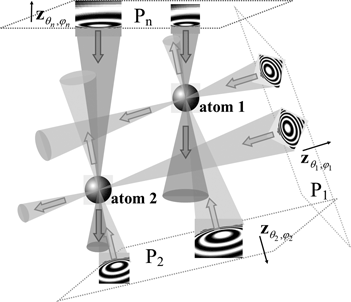
In CHR, as in the general DT approach, the effect of Fresnel diffraction in the course of image formation is accounted for by means of Fresnel backpropagation of a complex amplitude from each of the defocus planes onto multiple planes in the reconstructed volume, before averaging the partial reconstructions over all available illumination directions (Fig. 1). The numerical Fresnel backpropagation allows one to exploit the Ewald sphere curvature (shallow depth of field) and achieve a non-trivial localization of the atomic positions inside the reconstructed volume along the illumination direction in each partial reconstruction from a single defocused image (Figs. 2, 3). A number of alternative approaches for taking the Ewald sphere curvature into account have been suggested in recent years (DeRosier, Reference DeRosier2000; Wolf et al., Reference Wolf, DeRosier and Grigorieff2006; Russo & Henderson, Reference Russo and Henderson2018; Zivanov et al., Reference Zivanov, Nakane, Forsberg, Kimanius, Hagen, Lindahl and Scheres2018; Glaeser, Reference Glaeser2019; Chen et al., Reference Chen, Schmidt, Spence and Kirian2021). As shown in these publications, the effect of Ewald sphere curvature on the quality of 3D reconstruction becomes significant only at high spatial resolutions. Figure 2 indicates that, when used in high-energy electron imaging, the CHR technique is also likely to produce results that are superior to conventional CT-based techniques only at spatial resolutions finer than approximately 2 Å (the relevant details can be found in Appendix A).
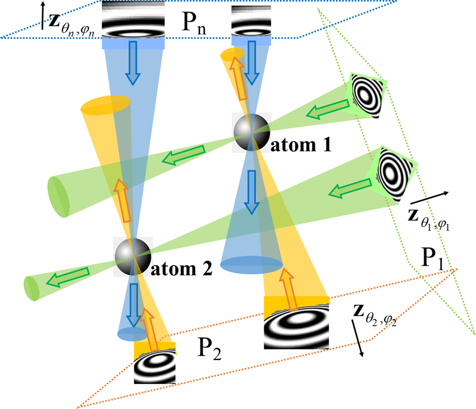
Fig. 1. Schematic representation of the CHR algorithm. Images are collected in an experiment at defocus planes P 1, P 2, … , Pn, at different orientations (illumination directions)  ${\bf z}_{\theta _1, \varphi _1}$, ${\bf z}_{\theta _2, \varphi _2}$, … , ${\bf z}_{\theta _n, \varphi _n}$. Fragments of idealized defocused images of two atoms are shown in each image plane. The waves with conjugated retrieved phases (shown as cones of different colors), backpropagating from these planes, are calculated numerically. The wide arrows in the figure indicate the backpropagation directions. These numerically calculated waves converge in the vicinity of individual atoms, creating strong peaks in the resultant signal, leading to efficient localization of the atoms in the reconstruction.

Fig. 2. CHR longitudinal point-spread functions (LPSFs), that is, the normalized backpropagation contrast functions at the central point (0, 0) of transverse (x θ,φ, y θ,φ) slices through the reconstructed 3D distribution of the electrostatic potential at different positions along the optic axis  ${\bf z}_{\theta , \varphi }$ which corresponds to a given illumination direction described by angles θ and φ. The multislice forward simulations, followed by the CHR, were performed for a single carbon atom located at the origin of coordinates and imaged with a plane monochromatic electron wave with E = 300 keV, spherical aberration C 3 = 2.7 mm, defocus distance of D θ,φ = 5,000 Å, and pixel size of 0.457 Å, at different effective spatial resolutions equal to 2 Å (blue curve), 1.5 Å (green curve), 1 Å (orange curve), and 0.5 Å (gray curve). Shifting each curve to the left by the corresponding distance d max moves the maximum to the position of the atom. Backprojected amplitude corresponding to conventional CT reconstruction is also shown (dotted purple line). See details in Appendix A.

Fig. 3. One-dimensional transverse profiles (along the y θ,φ coordinate) of the electrostatic potential at the z-position of a carbon atom which was located either at the geometric center of the reconstruction volume (z θ,φ = 0) or away from the center along the illumination direction (at z θ,φ = 60 Å). The profiles were reconstructed in each case from a single defocused image obtained using multislice forward simulations, with a plane monochromatic electron wave illumination with E = 300 keV, spherical aberration C 3 = 2.7 mm, defocus distance of D θ,φ = 10,000 Å, and the effective spatial resolution of 0.5 Å (limited by the objective aperture of 20 mrad). The CHR backpropagation results are shown by the red dashed curve (for the atom at z θ,φ = 0) and the black dotted curve (for the atom at z θ,φ = 60 Å), the two curves being almost identical. The CTF-corrected CT backprojection results are shown by the purple dashed curve (for the atom at z θ,φ = 0) and the purple dotted curve (for the atom at z θ,φ = 60 Å). The latter result shows significant broadening, lowering, and distortion of the reconstructed atomic potential.
When the Fresnel diffraction inside the sample is ignored and the projection approximation is used for the 3D reconstruction, the whole sample is effectively mapped onto a single plane orthogonal to the illumination direction at each view angle, as is clearly illustrated in reciprocal space by the Fourier slice theorem (Crowther et al., Reference Crowther, DeRosier and Klug1970; Born & Wolf, Reference Born and Wolf1999; Natterer, Reference Natterer2001). The equivalent picture in real space is that of “backprojection,” that is, the uniform “spreading” of the image contrast along straight rays passing through the sample volume, as implemented for example in the Filtered Backprojection (FBP) reconstruction method of conventional CT (Natterer, Reference Natterer2001). This indicates that the longitudinal spatial resolution which determines the position of different atoms inside the sample along the optic axis (i.e., the view direction) is as coarse as the total thickness of the sample (see the dotted purple line in Fig. 2). The spatial resolution in CT only improves after the partial reconstructions obtained at different illumination directions are added together. Note that this does not contradict the idea of using the CTF correction in a CT-based reconstruction (Cowley, Reference Cowley1995; Scheres, Reference Scheres2012; Grigorieff, Reference Grigorieff2016). Indeed, as mentioned above, the CTF correction accounts for the effect of free-space propagation of the transmitted electron beam from the imaged molecule to the detector, but it does not account for the propagation of the beam inside the molecule, because, for each defocused image, a single CTF correction is applied to all atoms in the molecule, regardless of their positions along the optic axis. In contrast, in the DT approach in general and in CHR in particular, multiple CTF corrections are effectively applied to each defocused image in accordance with the propagation distances from different transverse planes inside the volume occupied by the molecule to the detector. This allows one, under suitable circumstances, to resolve the longitudinal positions of different atoms in the molecule from a single image by locating the peaks of the “longitudinal point-spread function” (LPSF) (Fig. 2). This constitutes the first potential benefit offered by the CHR method in high-resolution TEM reconstruction of single molecules or nanoparticles. Note that by LPSF we denote a one-dimensional function L(z) = PSF(x, y, z), where z corresponds to the direction of the optic axis and PSF(x, y, z) is the conventional point-spread function.
A related benefit is provided by the CHR method in the reconstruction of the 3D electrostatic potential in a molecule or nanoparticle from multiple defocused images collected at different orientations. Here, the CHR method is capable of reducing the blurring of the electrostatic potential which may occur in conventional CTF-corrected CT reconstruction in the vicinity of atoms located far away from the center of rotation (i.e., on the periphery of the reconstructed volume). As the conventional CTF correction uses a single defocus distance for all atoms in the particle at each orientation, the atoms on the periphery of the particle are effectively treated in this method using a defocus distance that can be off by as much as half of the thickness of the particle. Consequently, when the thickness of the particle is large compared to the depth of field, this can lead to a noticeable broadening and distortion of the reconstructed atomic potentials. One such example is presented in Figure 3 for a carbon atom inside a simulated “particle volume” with a diameter of 138 Å which corresponds, for example, to the size of the apoferritin molecule 7KOD (Sun et al., Reference Sun, Azumaya, Tse, Frost, Southworth, Verba, Cheng and Agard2020, Reference Sun, Azumaya, Tse, Bulkley, Harrington, Gilbert, Frost, Southworth, Verba, Cheng and Agard2021). It can be observed in Figure 3 that while the CTF-corrected CT result for an atom located at the center of the particle volume is accurate, the corresponding result for an atom located on the periphery exhibits significant blurring and distortion due to the incorrect effective propagation distance. Indeed, the CTF correction was performed using the fixed defocus distance of 10,000 Å for the whole particle volume, while the atom located at 60 Å downstream from the center of the volume had the actual defocus distance of 9,940 Å. In contrast, the CHR method delivers accurate results for both the central and the peripheral positions of the atom using the same defocus distance of 10,000 Å. This is achieved in the CHR method via the use of multiple backpropagation planes in the reconstruction of the potential inside the particle, with the highest magnitude and the narrowest transverse distribution of the reconstructed signal always appearing at the correct longitudinal position for each atom (see Figs. 1, 2). Note that the actual different defocus distances for different atoms in the reconstructed particle are certainly not assumed to be known a priori in the CHR method. Instead, they are reconstructed in CHR from the average defocus distance given for the whole particle and the information intrinsically contained in the contrast of the defocused images.
In conventional CT-based reconstruction, the achievable spatial resolution directly depends on the range of available view angles. The Nyquist sampling conditions for uniform 3D spatial resolution in conventional CT require that the number of view angles, n a, is commensurate with the number of resolvable effective pixels in each detector row, nx, as for example n a = (π/2)n x in the case of plane-wave illumination and a 180 degree rotation scan (Natterer, Reference Natterer2001). In contrast to this situation, in conventional CT, the longitudinal resolution in each partial reconstruction from a single view angle in DT is proportional to the depth of field, and it can already provide some information about the localization of different elements in the sample along the view direction from a single projection, even before the angular summation (Hovden et al., Reference Hovden, Ercius, Jiang, Wang, Yu, Abruña, Elser and Muller2014). In particular, under suitable conditions in CHR, the single-view LPSF can approximate the Dirac delta-function (Fig. 2), negating the need for any filtering in the 3D reconstruction. The summation over different view angles in CHR acts as a simple averaging (Fig. 1) which increases the signal-to-noise (SNR) in the reconstruction and reduces some artifacts, as explained below. This allows the Nyquist sampling conditions for the number of view angles in a scan to be significantly relaxed. Ultimately, under suitable conditions, with a sufficiently shallow depth of field and a sufficiently “sparse” sample, where different spatially localized components (such as, e.g., individual atoms) do not shade each other along the rays of a given view, the whole 3D structure can be accurately reconstructed in CHR from a single view, similar to the way demonstrated previously in the Big Bang Tomography method (van Dyck et al., Reference Van Dyck, Jinschek and Chen2012; Chen et al., Reference Chen, Van Dyck and Kisielowski2016, Reference Chen, Warner, Kirkland, Chen and Van Dyck2017). The “non-shading” condition is related to the problem of multiple scattering (Brown et al., Reference Brown, Chen, Weyland, Ophus, Ciston, Allen and Findlay2018; Ren et al., Reference Ren, Ophus, Chen and Waller2020; Donatelli & Spence, Reference Donatelli and Spence2020; Gureyev et al., Reference Gureyev, Quiney, Kozlov, Paganin, Schmalz, Brown and Allen2021). When two atoms are located in close proximity along the same illuminating ray, the second atom will be “shaded” by the first one and hence cannot be considered illuminated by the initial unperturbed wave as assumed in the single-scattering first Born approximation (Born & Wolf, Reference Born and Wolf1999).
While DT is superior to conventional CT in that it takes the in-sample free-space propagation (Ewald sphere curvature) explicitly into account, DT techniques are usually based on the first Born or first Rytov approximation (Wolf, Reference Wolf1969; Devaney, Reference Devaney1982; Gbur & Wolf, Reference Gbur and Wolf2002). Correspondingly, they generally do not incorporate the effects of multiple scattering into their underlying models. However, in the case of CHR, the summation over different view angles strongly mitigates the multiple scattering contributions by averaging them out. The latter happens because in the majority of real-life samples multiple scattering tends to be highly directional, and hence, it averages out into a low quasi-uniform “background” during the angular averaging. On the other hand, the single-scattering cross-section tends to be relatively uniform with respect to the illumination directions (due to the spherical symmetry of the atomic potential), which leads to a positive reinforcement of the single-scattering signal in the process of angular averaging in CHR. In particular, the angular averaging relaxes the “non-shading” condition mentioned above, as, for example, two adjacent atoms in a molecule cannot shade each other along all possible illumination angles. This two-atom case represents the simplest example explaining the directional nature of multiple scattering and the reasons for the contribution of multiple-scattering effects to weaken when the images collected at different illuminating directions are utilized in a 3D reconstruction (Ciston et al., Reference Ciston, Deng, Marks, Own and Sinkler2007). More sophisticated approaches to 3D reconstruction have been developed in recent years which explicitly take multiple scattering into account (Van den Broek & Koch, Reference Van den Broek and Koch2012; Ren et al., Reference Ren, Ophus, Chen and Waller2020; Du et al., Reference Du, Kandel, Deng, Huang, Demortiere, Nguyen, Tucoulou, De Andrade, Jin and Jacobsen2021). While these approaches can certainly produce more quantitatively accurate results compared to DT-based methods in the presence of strong multiple scattering, they tend to be more computationally demanding. Convergence to the “global minimum” may also become a problem if the input data is very noisy, incomplete, or internally inconsistent. It may be interesting to investigate in the future an option of using a simple non-iterative DT-based solution, like the one described in the present paper, as an initial approximation for these more sophisticated reconstruction approaches.
Another common challenge with DT methods is the need to know the complex amplitude of the diffracted wave in the detector plane at each view angle. This is necessary in order to perform the Fresnel backpropagation step of the DT reconstruction process, which replaces the backprojection step of conventional CT. In a typical experiment, only the intensity distribution of the transmitted beam is registered at each view angle. The phase needs to be retrieved from these intensity images, possibly with the help of available a priori information. When several images at different propagation (defocus) distances are available at a given view (illumination) angle, various phase-retrieval methods, such as, for example, the Iterative Wave Function Reconstruction (IWFR) method (Allen et al., Reference Allen, McBride, O'Leary and Oxley2004) or the method based on L2-difference minimization of the CTF (Paganin et al., Reference Paganin, Barty, McMahon and Nugent2004) can be applied. The problem of phase retrieval from a single image per view angle is much more challenging in general, although some potentially suitable methods have been suggested (Morgan et al., Reference Morgan, Martin, D'Alfonso, Putkunz and Allen2011). In the present work, we propose a new method for phase retrieval from a single defocused image per view angle, which is suitable under the first Born approximation. However, crucially, we also show that backpropagation with the “true” phase is not necessarily the most effective method for 3D reconstruction from complex amplitudes available at different view angles. We demonstrate both theoretically and in numerical simulations that using instead a numerically “conjugated” phase (i.e., the phase with the opposite sign) can lead to a better-localized LPSF (Fig. 2) and hence to a higher-quality reconstruction. The idea of phase conjugation in holographic imaging has been discussed previously (Nieto-Vesperinas, Reference Nieto-Vesperinas2006), however, to the best of our knowledge, it has not been previously considered in the context of DT-type reconstructions.
Three-Dimensional Transmission Imaging and Reconstruction Models
As mentioned in the Introduction, the CHR method is based on the general DT approach. CHR is closely related to the earlier DHT method (Gureyev et al., Reference Gureyev, Quiney, Kozlov and Allen2020, Reference Gureyev, Quiney, Kozlov, Paganin, Schmalz, Brown and Allen2021), with the key difference being the phase conjugation used in CHR, as described below. The present version of CHR is introduced in the context of the first Born approximation, but the first Rytov approximation can be used instead, if preferred. Compared to the generic DT formalism, the CHR technique has the following distinguishing features.
(1) The imaged sample is modeled as a set of independent atoms (or possibly other localized components), with each defocused image treated as an incoherent sum of contributions produced by the interference between the incident wave and the wave scattered by one atom. The “independent atom model” is used in the reconstruction scheme of CHR as well.
(2) Particular forms of phase retrieval and phase conjugation are applied at each of the defocus planes using a single intensity image.
(3) An additional longitudinal offset d max, which can be estimated a priori for a given imaging setup, is introduced in the reconstruction, effectively moving the peaks of the LPSFs to the atomic positions (see details in Appendix A). Remarkably, this optimal offset is independent of the distances between different atoms in the imaged structure and the detector plane.
These key points are expanded and explained below, leading to the central new result, equation (4), which describes the proposed CHR algorithm.
Let us introduce the necessary notation and outline the overall physical picture and key assumptions used in the imaging model underlying the DHT and CHR methods. A monochromatic plane wave  $I_{{\rm in}}^{1/2} \exp ( { i}2\pi kz)$ is assumed to illuminate a weakly scattering object, where k = 1/λ is the wave number, I in is the uniform intensity of the incident wave, ${\bf r}\equiv ( x, \;y, \;z)$ is a Cartesian coordinate system in 3D space and z is the direction of the optic axis. The interaction of the incident wave with the imaged object is determined by the refractive index n(r). In the case of electron microscopy, we have $n( {\bf r}) \cong 1 + V( {\bf r}) /( 2E) ,$ where $V( {\bf r}) \ge 0$ is the electrostatic potential, E is the relativistically corrected accelerating voltage, with $\alpha \equiv \max \vert V( {\bf r}) /( 2E) \vert$ typically being much less than unity (Sanchez & Ochando, Reference Sanchez and Ochando1985; Allen & Rossouw, Reference Allen and Rossouw1990). The complex amplitude U(r) of the wave inside the object satisfies the time-independent Schrödinger equation: $\nabla ^2U( {\bf r}) + 4\pi ^2n^2( {\bf r}) k^2U( {\bf r}) = 0$. We consider the problem of reconstruction of the 3D distribution of the electrostatic potential from the intensity of transmitted waves measured at some distance from the object along the optic axis (i.e., from defocused images), for a number of different orientations of the object.
In the model used in DHT and CHR, the first Born approximation is applied for solution of the above Schrödinger equation. The perturbation of the wave incident on a particular atom by other atoms in the specimen is neglected. The free-space propagation (Fresnel diffraction) of the waves scattered from individual atoms, as these scattered waves propagate through the object, is taken into account. The intensity of the projection image collected at a position, z, downstream from the object along the optic axis is expressed as an incoherent sum of (i) the primary beam intensity and (ii) the interference terms between the scattered wave from each atom and the incident plane wave (Voortman et al., Reference Voortman, Stallinga, Schoenmakers, van Vliet and Rieger2011; Gureyev et al., Reference Gureyev, Quiney, Kozlov and Allen2020). The terms corresponding to the interference of the waves scattered by different atoms are of the second order (α 2) with respect to the small parameter α in the Born series and are neglected.
The 2D Fourier transform of the defocused images  $I( {\bf r}_\bot , \;z) \equiv \vert U( {\bf r}_\bot , \;z) \vert ^2$, with ${\bf r}\equiv ( {\bf r}_\bot , \;z)$ and ${\bf r}_\bot \equiv ( x, \;y)$, can be written as (Gureyev et al., Reference Gureyev, Quiney, Kozlov and Allen2020)
 $$\eqalign{( {\bf F}_2I) ( {\bf q}_\bot , \;z) /I_{\rm {in}} & = \delta ( {\bf q}_\bot ) + [ 2\pi {\rm /( }\lambda E) ] \cr & \times \int {\sin [ \pi \lambda ( z-{z}^{\prime}) q_\bot ^2 ] ( {\bf F}_2V) ( {\bf q}_\bot , \;{z}^{\prime}) d{z}^{\prime}, }}$$
where  $( {\bf F}_2f) ( {\bf q}_\bot ) \equiv \int\!\!\!\int {\exp ( {-}i2\pi {\bf q}_\bot {\bf r}_\bot ) f( {\bf r}_\bot ) d{\bf r}_\bot }$ is the 2D Fourier transform with respect to the transverse coordinates, ${\bf q}\equiv ( {\bf q}_\bot , \;q_z)$, ${\bf q}_\bot \equiv ( q_x, \;q_y)$, and $q_\bot \equiv \,\vert {\bf q}_\bot \vert$. Equation (1) has the form of an incoherent sum of the well-known expressions for the first Born approximation to the scattered intensities (Cowley, Reference Cowley1995) corresponding to different transverse planes, z′, inside the imaged object.
The image intensities are assumed to have been measured in defocused planes for different 3D rotational orientations of the imaged object. An arbitrary illumination direction in 3D can be represented, for example, as a result of a rotation of a wave, initially traveling along z, around the y-axis by an angle θ ∈ [0, π) followed by a rotation around the  $x_\theta$ axis by an angle φ ∈ [0, 2π):
 $${\left\{\matrix{x_{\theta , \varphi } = x_\theta = x\sin \theta + z\cos \theta \hfill \cr y_{\theta , \varphi } = y_\theta \cos \varphi + z_\theta \sin \varphi -y\cos \varphi -x\cos \theta \sin \varphi + z\sin \theta \sin \varphi \hfill \cr z_{\theta , \varphi } = {-}y_\theta \sin \varphi + z_\theta \cos \varphi = {-}y\sin \varphi -x\cos \theta \cos \varphi + z\sin \theta \cos \varphi. \hfill} \right.}$$
 Accordingly, we use the notation  ${\bf r}_{\theta , \varphi }\equiv ( x_{\theta , \varphi }, \;y_{\theta , \varphi }, \;z_{\theta , \varphi }) = ( {\bf r}_{\theta , \varphi , \bot }, \;z_{\theta , \varphi })$. In addition to arbitrary illumination directions, which are defined by the two Euler angles θ and φ, the imaged object can be rotated around the illumination axis z θ,φ by some angle ψ. Note that in the simulations included in the section “Results” below a different set of Euler angles is used to define the 3D orientations in accordance with the conventions described in Heymann et al. (Reference Heymann, Chagoyen and Belnap2005), but it does not change the theory as described here. In DHT and CHR, all available images corresponding to a particular illumination direction z θ,φ are pre-processed numerically, rotating these images around the axis z θ,φ toward some fixed angle ψ, such as ψ = 0. Subsequently, the algorithm is applied to the intensity distributions $I_{\theta , \varphi }( {\bf r}_{\theta , \varphi , \bot }, \;z_{\theta , \varphi }) \equiv I_{\theta , \varphi , \psi = 0}( {\bf r}_{\theta , \varphi , \bot }, \;z_{\theta , \varphi })$. Therefore, the input data in DHT and CHR are considered as consisting of a set of 2D distributions $I_{\theta , \varphi }( {\bf r}_{\theta , \varphi , \bot }, \;D_{\theta , \varphi , l}) ,$ corresponding to defocus planes z θ,φ = D θ,φ,l at different illumination directions indexed by the angles θ and φ and at different defocus distances indexed by l = 1, 2, …, L θ,φ. The most practically important case considered below corresponds to a single defocused image per illumination direction, that is, to the case L θ,φ = 1 at all θ and φ.
A suitable phase-retrieval procedure can produce a phase distribution  $\Phi _{\theta , \varphi }( {\bf r}_{\theta , \varphi , \bot }, \;D_{\theta , \varphi })$ from a single measured intensity $I_{\theta , \varphi }( {\bf r}_{\theta , \varphi , \bot }, \;D_{\theta , \varphi })$ at each defocus plane z θ,φ = D θ,φ (or, optionally, from multiple images collected at a given illumination direction). Relevant details of the single-image phase-retrieval process are discussed in Appendix A. In DHT, the resultant 2D complex amplitude $U_{\theta , \varphi }( {\bf r}_{\theta , \varphi , \bot }, \;D_{\theta , \varphi }) \equiv I_{\theta , \varphi }^{1/2} ( {\bf r}_{\theta , \varphi , \bot }, \;D_{\theta , \varphi }) \exp [ i\Phi _{\theta , \varphi }( {\bf r}_{\theta , \varphi , \bot }, \;D_{\theta , \varphi }) ]$ is numerically backpropagated into the 3D volume containing the imaged object by calculating the corresponding Fresnel integrals and producing the complex amplitudes $U( {\bf r}_{\theta , \varphi , \bot }, \;z_{\theta , \varphi })$ at different transverse planes with z = z θ,φ inside the object. We introduce the backpropagated contrast function, $K( {\bf r}_{\theta , \varphi , \bot }, \;z_{\theta , \varphi }) \equiv 1-I( {\bf r}_{\theta , \varphi , \bot }, \;z_{\theta , \varphi }) /I_{in}$, where $I( {\bf r}_{\theta , \varphi , \bot }, \;z_{\theta , \varphi }) \equiv \vert U( {\bf r}_{\theta , \varphi , \bot }, \;z_{\theta , \varphi }) \vert ^2$ is the intensity of the numerically backpropagated beam. The DHT reconstruction formula for the electrostatic potential can then be written as (Gureyev et al., Reference Gureyev, Quiney, Kozlov, Paganin, Schmalz, Brown and Allen2021)
 $$V( {\bf r} ) \cong {\rm \;}\displaystyle{E \over {8\pi wd}}\nabla ^{{-}2}\int_0^{2\pi } {\int_{-\pi }^\pi {K_{\theta , \varphi }( {\bf r}_{\theta , \varphi , \bot }, \;z_{\theta , \varphi } + d) \vert \sin \varphi \vert d\theta } d\varphi } , $$
where w is a constant “atom width” parameter (which is usually taken to be 1 Å for low-Z atoms), d is a specially introduced offset parameter, and  $\nabla ^{{-}2}$ is the inverse Laplacian operator, such that $( \nabla ^{{-}2}f) ( {\bf r}) \equiv{-}( {\bf F}_3^{{-}1} \vert {\bf q}\vert ^{{-}2}{\bf F}_3f) ( {\bf r})$. As this operator has a singularity at ${\bf q} = 0$, it usually requires a regularization in a vicinity of the zero frequency in practical applications, for example, by replacing $\vert {\bf q}\vert ^{{-}2}$ with $( \vert {\bf q}\vert ^2 + a^2) ^{{-}1}$, where a is a small constant. Note that the integration over θ in equation (3) is performed over the interval ( −π, π), rather than (0, π), as is usually done in parallel-beam CT (Natterer, Reference Natterer2001). This is a consequence of the fact that the DHT reconstruction, equation (3), relies on pair-wise combinations of the backpropagated contrast functions corresponding to opposed illumination directions (Gureyev et al., Reference Gureyev, Quiney, Kozlov, Paganin, Schmalz, Brown and Allen2021). The fact that the unit sphere is then covered twice in the integration in equation (3) leads to the normalization factor 8π in the denominator, that is, twice the area of the unit sphere in 3D. The inverse Laplace operator in equation (3) accounts for the local “offset contrast” which appears in the vicinity of individual atoms after addition of pairs of contrast functions backpropagated from the opposed directions. This contrast has a similar physical nature to the propagation-induced phase contrast in the near-Fresnel region which is described by the Transport of Intensity equation (Teague, Reference Teague1983; Paganin, Reference Paganin2006).
The inverse Laplacian is omitted from the DHT reconstruction formula when phase conjugation is applied to the measurement-plane complex amplitude prior to backpropagation in the CHR method, as explained in Appendix A. In the case of the backpropagated wave with the conjugated phase, we denote the backpropagated intensity distribution as  $\tilde{I}( {\bf r}_{\theta , \varphi , \bot }, \;z_{\theta , \varphi })$, with $\tilde{K}( {\bf r}_{\theta , \varphi , \bot }, \;z_{\theta , \varphi }) \equiv 1-\tilde{I}( {\bf r}_{\theta , \varphi , \bot }, \;z_{\theta , \varphi }) /I_{\rm in}$ being the corresponding contrast function. The CHR formula for the 3D potential then takes the following form:
 $$V( {\bf r} ) \cong \displaystyle{{-E\lambda \gamma } \over {4\pi ^2w}}\int_0^{2\pi } {\int_0^\pi {{\tilde{K}}_{\theta , \varphi }( {\bf r}_{\theta , \varphi , \bot }, \;z_{\theta , \varphi } + d_{\max }) \vert \sin \varphi \vert d\theta } d\varphi } ,$$
where γ is a dimensionless constant that is equal to approximately 0.1 when imaging molecules consisting of light chemical elements with high-energy electrons of energy E ≅ 200−300 keV (see Appendix B for details) and d max is the distance between the maximum of the function  $\tilde{K}( {\bf r}_{\theta , \varphi , \bot }, \;z_{\theta , \varphi })$ along the optic axis z θ,φ and the atomic locations along that axis (see Fig. 2). It is shown in Appendix B that, for a given imaging setup, the distance d max is the same for all atoms in the imaged molecule and can be estimated numerically. Equation (4) is usually not very sensitive to small errors in the estimation of d max, because of the relatively broad maxima of the LPSF curves at atomic resolutions, as can be seen in Figure 2. The CHR method, as expressed by equation (4), no longer relies on the pair-wise combinations of the backpropagated contrast functions corresponding to opposed illumination directions. Accordingly, the integration over θ in equation (4) is performed over the interval (0, π), with the corresponding normalization factor 4π in the denominator. Note also that when the inverse Laplacian in equation (3) is strongly regularized in order to optimally handle the division by zero in the Fourier space, equation (3) effectively converges to equation (4).
In general, equations (3) and (4) represent a form of angular averaging of the 3D backpropagated contrast distributions,  $K( {\bf r}_{\theta , \varphi , \bot }, \;z_{\theta , \varphi } + d)$ or $\tilde{K}_{\theta , \varphi }( {\bf r}_{\theta , \varphi , \bot }, \;z_{\theta , \varphi } + d_{\max })$, over the illumination angles θ and φ. The factor |sinφ| accounts for the fact that the area element on a unit sphere in 3D is equal to |sinφ|dθdφ. In other words, a uniform sampling of the angle φ does not correspond to uniform sampling of the illumination space (i.e., the unit sphere in 3D) and, hence, requires the “correction” factor |sinφ|. In practice, if the input data already corresponds to uniform sampling of the unit sphere (which means, in particular, that the sampling of the angle φ is not uniform), this correction factor is omitted, with the reconstruction obtained simply by angular averaging of the (rescaled) backpropagated contrast distributions $K_{\theta , \varphi }( {\bf r}_{\theta , \varphi , \bot }, \;z_{\theta , \varphi } + d)$. A schematic representation of the CHR method is shown in Figure 1. Note that, unlike conventional CT, equations (3) and (4) do not contain any radial filtering. As explained in the Introduction, this happens because the LPSF of CHR has a high degree of localization along the backpropagation directions z θ,φ.
The mathematical details of the CHR algorithm are given in the Appendices, together with the relevant physical and optical considerations. A reader not interested in these details can simply note the main formula describing the algorithm, that is, equation (4) above, and proceed to examples of the application of this method in the section “Results.”
Results
Here, we present the results of numerical tests of the CHR algorithm based on equation (4). Related simulation results based on the DHT algorithm, equation (3), can be found in our earlier publications (Gureyev et al., Reference Gureyev, Quiney, Kozlov and Allen2020, Reference Gureyev, Quiney, Kozlov, Paganin, Schmalz, Brown and Allen2021). Here, we use the conditions, such as the electron beam energy, defocus distances, and microscope aberrations, similar to those found in high-resolution TEM experiments. In the definition of the main parameters used in the simulations below, we adhere to the conventions outlined in Heymann et al. (Reference Heymann, Chagoyen and Belnap2005).
Apoferritin Molecule (7KOD)
Our first example of CHR application uses a molecular structure based on the heavy chain mouse apoferritin molecule 7KOD (Sun et al., Reference Sun, Azumaya, Tse, Frost, Southworth, Verba, Cheng and Agard2020, Reference Sun, Azumaya, Tse, Bulkley, Harrington, Gilbert, Frost, Southworth, Verba, Cheng and Agard2021) downloaded from the Protein Data Bank. Apoferritin is a protein for storing iron in the liver. It has become a favorite for pushing the boundaries of cryo-EM due to the fact that it is a very rigid molecule that does not vibrate much under the beam (Nakane et al., Reference Nakane, Kotecha, Sente, McMullan, Masiulis, Brown, Grigoras, Malinauskaite, Malinauskas, Miehling, Uchański, Yu, Karia, Pechnikova, de Jong, Keizer, Bischoff, McCormack, Tiemeijer, Hardwick, Chirgadze, Murshudov, Aricescu and Scheres2020). The molecular structure used in this simulation contained 66,459 atoms in total (S192O6480N5928C21216H32643), including 33,816 non-hydrogen atoms. At each orientation, we also added a 166 Å thick layer of pseudo-randomly distributed water molecules simulating amorphous ice, using the code adopted from Kirkland (Reference Kirkland2021). The combined structures containing the apoferritin molecule and the random ice layer contained more than 320,000 atoms at each orientation. We assumed that the structure was illuminated by a plane monochromatic electron wave with E = 300 keV. The “forward” simulations comprised of 1,000 defocused images of these structures, each image containing 512 × 512 of ~0.27 × 0.27 Å2 pixels, obtained at different defocus distances of around 1.3 μm, with a fixed spherical aberration C 3 = 2.7 mm, simulated random astigmatism and random transverse (x–y) shifts of the order of 10 Å. The images were created at random 3D orientations of the molecular structure, defined by the three Euler angles (Heymann et al., Reference Heymann, Chagoyen and Belnap2005). The orientation and defocus data for these simulations were imported from RELION software (Scheres, Reference Scheres2012; Zivanov et al., Reference Zivanov, Nakane, Forsberg, Kimanius, Hagen, Lindahl and Scheres2018) where it was generated in the course of analysis of a real cryo-EM experimental dataset. We also incorporated the effect of thermal motion of atoms via a Debye–Waller factor (Cowley, Reference Cowley1995) corresponding to a root-mean-square displacement of 0.1 Å at 300 K, scaled down according to the assumed temperature of 77 K (−196°C). We did not include any electron shot noise in the simulated images in this example, as, with the current parameters, it would have required many more images for a high-quality 3D reconstruction, leading to a prohibitively long computation time in the forward simulation step. The forward multislice-based simulations using our optimized C++ code (Gureyev, Reference Gureyev2021) took approximately 24 h on a PC with dual Xeon Gold 6149 processors, running 64 parallel threads at close to 100% CPU load at all times to calculate the 1,000 defocused images. An example in the section “RNA polymerase molecule (7AAP)” below, which involves a smaller molecule, demonstrates the effect of realistic amounts of electron shot noise on the CHR result obtained from 10,000 defocused images. Note however that the simulated random layer of ice already has effectively introduced large amounts of image “noise” in the present example. A typical defocused image is shown in Figure 4a. Figure 4b contains a low-pass filtered copy of an experimental cryo-EM image of apoferritin for comparison.

Fig. 4. (a) Simulated defocused image of apoferritin structure embedded in amorphous ice. (b) A low-pass filtered experimental cryo-EM image of an apoferritin molecule. (c) A typical cross-section through the 3D potential distribution obtained using CHR. (d) A filtered and thresholded version of the same slice as in (c).
We applied the CHR algorithm based on equation (4) with w = 1 Å and d max = 10 Å to the 1,000 simulated defocused images. The reconstruction cube had a side of 138 Å, as needed to enclose the 7KOD structure. The whole reconstruction using our software (Gureyev, Reference Gureyev2021) took less than 1 h on the same computer hardware as described above. A typical cross-section through the 3D potential obtained with CHR is shown in Figure 4c. Many atomic positions can be easily identified in this reconstructed image. After that, we high-pass filtered the reconstructed 3D potential by subtracting a 10-pixel-wide Gaussian-averaged copy from it. The filtered potential was then thresholded from below with the minimum cut-off level of 0.3 V. An image of the same slice of the filtered and thresholded 3D potential is shown in Figure 4d. Finally, we applied a simple peak-localization algorithm [as implemented in our software (Gureyev, Reference Gureyev2021)] to the filtered potential distribution, which resulted in 34,924 identified peaks (reconstructed atomic positions).
Having reconstructed the atomic positions in the imaged molecule, we then matched the located atomic positions with the original ones in the initial structure file used for the forward simulations (with the hydrogen atoms removed). The matching was based on pair-wise distance minimization, that is, for each atom in the original structure, we identified one atomic location in the reconstructed set that had a minimal distance from the given original atom. If that minimal distance was larger or equal to a set limit (in this case, 1.0 Å), then the match was discarded, resulting in what we termed a “false negative” (missed atom) instance. We repeated this procedure for each atom in the original structure. At the end of this procedure, some atomic locations in the reconstructed set had not been matched with any atoms in the original structure. These remaining reconstructed locations were called “false positives,” referring to the localized “atoms” in places where the original structure actually had none. The whole matching procedure was performed using the routine “pdb-compare” from our software package (Gureyev, Reference Gureyev2021). As a result, 33,540 out of a total of 33,816 atoms (99.18%) were uniquely matched, with the average distance between the matched reconstructed and original atomic positions equal to 0.14 Å and a maximum distance of 0.996 Å. There were 276 “false negative” results, that is, 0.82% of the total number of original atoms, and 1,384 “false positive” results (localized “atoms” in places where the original structure had none), that is, 3.96% of the total.
RNA Polymerase Molecule (7AAP)
Our second simulation test included the SARS-CoV-2 RNA-dependent RNA polymerase molecule in the presence of favipiravir-RTP, represented by the structure 7AAP from Protein Data Bank (Naydenova et al., Reference Naydenova, Muir, Wu, Zhang, Coscia, Peet, Castro-Hartman, Qian, Sader, Dent, Kimanius, Sutherland, Loewe, Barford and Russo2020, Reference Naydenova, Muir, Wu, Zhang, Coscia, Peet, Castro-Hartmann, Qian, Sader, Dent, Kimanius, Sutherland, Löwe, Barford and Russo2021). This structure contained 9,446 non-hydrogen atoms (Z2Fe1S66P26Mg3O1848N1581C5919). We also added a simulated layer of amorphous ice with 140 Å thickness at each orientation. The addition of ice resulted in over 250,000 extra atoms in each input structure, and the actual RNA polymerase molecule constituted only about 4% of atoms in the total simulated structures.
The “forward” simulations in this case contained 10,000 defocused images of the 7AAP structure with added ice, obtained with a plane electron wave illumination at E = 300 keV, with 256 × 256 of ~0.453 × 0.453 Å2 pixels in each image. The images were calculated under conditions similar to those described in the section “Apoferritin molecule (7KOD)” above, including the same fixed C 3 aberration, “random” astigmatism and thermal motion of atoms. However, in the present case, we also simulated the Poisson shot noise statistics in the detector at the level of 10 electrons per Å2, which resulted in a mean signal-to-noise ratio of approximately 1.4 in each simulated defocused image. Typical simulated defocused images before and after the addition of the shot noise are shown in Figures 5a and 5b, respectively. We used many more simulated images in this example, compared to the previous example (10,000 versus 1,000), because the high level of image noise used in the present example dictated the need to have more input images in order to achieve a successful CHR result. Note, however, that the 10,000 input images used in the current example are still at least an order of magnitude less than the number of input images in a typical high-resolution cryo-EM single-particle analysis experiment. We also reduced the number of image pixels by a factor of four in the present example compared to the previous example. This was done primarily in order to keep the computational time down in the forward simulations. This would have been difficult to replicate in the previous example, because of the larger number of atoms in the molecule analyzed in the section “Apoferritin molecule (7KOD),” compared to the molecule used in the present example. Even with the images having 256 × 256 pixels, it took approximately 28 h to simulate the 10,000 defocused images using the same software and the same computer hardware as described in the section “Apoferritin molecule (7KOD)”. In contrast, the subsequent application of CHR algorithm to the 10,000 simulated frames took only around 30 min to complete.

Fig. 5. (a) A typical simulated defocused image of 7AAP structure embedded in amorphous ice, before the addition of the shot noise. (b) Same as (a), but after the addition of the simulated shot noise at the level of 10 electrons per Å2 in each image. (c) A typical cross-section through the 3D potential distribution obtained using CHR. (d) A high-pass filtered version of the CHR reconstruction of the same slice obtained from 1,001 simulated defocused images with 1,024 × 1,024 pixels and 10 electrons per Å2. (e) Same as (d), but obtained using RELION 3.1 software with the Ewald sphere curvature correction option. (f) Same as (e), but without the Ewald sphere curvature correction.
We then applied the CHR algorithm based on equation (4) with w = 1 Å and d max = 10 Å to the 10,000 simulated noisy defocused images. A typical cross-section through the 3D potential obtained using CHR is shown in Figure 5c. As in the previous case, many atomic positions could be identified by eye in this “raw” reconstructed image. We subsequently high-pass filtered this 3D potential distribution by subtracting its copy convolved with a 10-pixel-wide Gaussian. The application of the peak localization algorithm to this filtered 3D potential distribution resulted in 9,444 atom localizations. A subsequent comparison of the reconstructed atom locations with the original atom positions in the 7AAP structure produced the following outcome: 9,184 atoms out of a total of 9,446 atoms in the 7APP structure (i.e., 97.23%) were uniquely matched. This result contained 262 false negatives (2.77%) and 309 false positives (3.26%). The average distance between the original and the reconstructed atomic positions was 0.35 Å, with a maximum distance of 0.997 Å and a standard deviation of 0.18 Å. All sulfur atoms and all but one of the phosphorus atoms present in the 7AAP structure were correctly located. There was no clear spatial pattern for the false negative results, that is, for the position of atoms in the original 7AAP structure that could not be located in the present CHR result.
We also compared the above CHR results for the 7AAP molecule with the corresponding results obtained using RELION 3.1 software (Scheres, Reference Scheres2012; Zivanov et al., Reference Zivanov, Nakane, Forsberg, Kimanius, Hagen, Lindahl and Scheres2018). In the first such attempt, we loaded the 10,000 simulated defocused images (described above), together with the information about their orientations, defocus distances, and other relevant parameters, into RELION and performed the reconstruction of the 3D electrostatic potential. In doing so, we applied the Ewald sphere curvature correction option in RELION, in particular Russo & Henderson (Reference Russo and Henderson2018) and Zivanov et al. (Reference Zivanov, Nakane, Forsberg, Kimanius, Hagen, Lindahl and Scheres2018). The resultant reconstructed potential had a significantly lower spatial resolution compared to the CHR result described above and shown in Figure 5c. Fourier shell correlation-based spatial resolution of this RELION reconstruction was 2.8 Å. We believe that the reason for this low resolution was that the present 10,000 simulated images had only 256 × 256 pixels each with the image size of 116 × 116 Å2. While the spatial resolution in the near-Fresnel region (where the inverse Fresnel number is small,  $N_F^{{-}1} \equiv ( \lambda z) /h^2 < < 1$, with h being the pixel size) is determined predominantly by the pixel size, in the far-Fresnel region (where $N_F^{{-}1} \equiv ( \lambda z) /h^2 > > 1$), the spatial resolution can be limited by either the pixel size or the image aperture (side length), A, with the required optimal relationship between the two being Ah ≅ λz, or $A\cong N_F^{{-}1} h$. In the current case, we had h = 0.453 Å, λ ≅ 0.02 Å, z ≅ 104 Å, $N_F^{{-}1} \cong 975$, and so the latter requirement translated into the aperture size of approximately 442 Å, which is significantly larger than the above image aperture of 116 Å. We hypothesize that the apparent high spatial resolution in the CHR result presented earlier in this section (e.g., Fig. 5c) was possible because of the intrinsic periodicity of the numerical Fast Fourier Transform (FFT) used in our simulations, both in the forward image calculation and in the CHR. As a result of this periodicity, the high-order diffraction fringes were “folded” back into the image across the opposite boundaries in the forward simulations, and the corresponding image contrast was implicitly utilized at the CHR stage. The same behavior could not be expected from the RELION reconstruction, which suffered from the lack of high-resolution information as a result.
In order to rectify this problem, we carried out additional simulations using defocused images with the aperture of 464 Å and 1,024 × 1,024 pixels. We simulated 1,001 of these larger defocused images of the 7AAP structure using the first 1,001 entries from the same orientation parameter file as before. We then added pseudo-random Poisson noise corresponding to 10 electrons per Å2 to the simulated images. Finally, we performed the retrieval of the 3D electrostatic potential distribution from these noisy images in the CHR software and in the RELION 3.1 software with and without the Ewald sphere curvature correction option. In this case, the reconstruction result from RELION with the Ewald sphere curvature correction was somewhat better than that obtained using CHR (see Figs. 5d, 5e). A comparison of the peak locations in the two reconstructions with the original XYZ file for the 7AAP structure led to sub-Å localization of 84.61% of atoms from the CHR potential and 85.94% for the RELION reconstruction. The same reconstruction in RELION without the Ewald sphere curvature correction resulted in sub-Å localization of 81.66% of atoms in the original 7AAP structure. It was apparent in these reconstructions that the RELION software managed image noise more effectively than our current implementation of the CHR algorithm which does not yet have any sophisticated tools for this purpose. We did apply both a high-pass Gaussian filter with 3.5 Å width (to remove the slowly varying background) and a low-pass Gaussian filter with 1 Å width (to filter out some noise) in the CHR reconstruction in this case, but this was certainly a much cruder tool compared to the Fourier shell correlation (FSC) curve-based spatial filtering used in cryo-EM. These results indicate that the CHR method provided an improvement in the accuracy of the 3D reconstruction compared to the RELION reconstruction without the Ewald sphere curvature correction, while the effect of the Ewald sphere curvature correction was moderate both in RELION and in CHR. The latter outcome can be explained by the fact that the spatial resolution in this simulated example was negatively affected by the relatively low number of input images and the high level of noise in them. The FSC-based estimation of the spatial resolution of the RELION reconstruction was 1.9 Å without the Ewald sphere curvature correction, and it improved only to 1.8 Å after the application of the Ewald sphere curvature correction option.
Overall, the present comparison tests between CHR and RELION should be considered preliminary and they may not yet correctly reflect the true performance potential of the two methods for Ewald sphere curvature correction. We plan to carry out further such tests using experimental cryo-EM datasets in the future. We will also make our test image sets of the 7AAP structure available to anyone on request (by sending an email to the first author), so that the interested reader could potentially perform their own comparison using RELION or other software for 3D reconstruction of the electrostatic potential.
Fe–Pt Nanoparticle
Our final simulation used a Fe–Pt nanoparticle with 5,107 Pt atoms and 5,356 Fe atoms (10,463 atoms in total). This particle can be fully enclosed in a cubic 3D volume with 70 Å sides. We also added a simulated amorphous carbon substrate in the form of a cube with 100 Å sides located just “under” the nanoparticle. The simulated substrate contained 90,253 C atoms, so the whole test structure consisting of the nanoparticle and the substrate contained 100,716 atoms. The structure was centered within a cubic volume with the linear dimension of 200 Å. This volume was sufficient to contain the whole test structure during arbitrary 3D rotations around the central point. Figure 6a presents a 3D rendering of the simulated test structure, produced using the Vesta software (Momma & Izumi, Reference Momma and Izumi2006) from the input XYZ file with atom positions.

Fig. 6. (a) 3D rendering of the Fe–Pt nanoparticle on the carbon substrate. (b) A typical simulated defocused image of the Fe–Pt nanoparticle on the carbon substrate with simulated shot noise at the level of 9 electrons per pixel. (c) A typical cross-section through the 3D potential distribution obtained using CHR in the part of the imaged volume containing the nanoparticle. (d) The result of peak localization in the slice shown in (c). (e) The original nanoparticle with the atoms not located by the CHR algorithm shown as larger green balls. (f) The same cross-section through the 3D potential as in (c), but reconstructed using the orientation and defocus parameters containing random errors.
The “forward” simulations in this case contained just 360 defocused images with 512 × 512 of 0.390625 × 0.390625 Å2 pixels each. The images were obtained with a plane monochromatic electron wave illumination with E = 200 keV. An objective aperture of 40 mrad and no spherical aberrations were imposed, approximating an aberration-corrected TEM. The effect of thermal motion of atoms was included in the simulations via a Debye–Waller factor with the root-mean-square displacement of 0.085 Å at 300 K. The images corresponded to 360 different illumination directions uniformly randomly distributed on the unit sphere in 3D, with one defocused image per orientation and with all defocus distances uniformly randomly distributed between 100 and 150 Å. We then added simulated Poisson shot noise with a mean of 9 electrons per pixel, which, given the pixel dimensions, corresponded to approximately 59 electrons per Å2 in each image. The latter number was equivalent to a total dose of 21,240 electrons per Å2 over the whole scan. A typical defocused image is shown in Figure 6b.
A CHR algorithm based on equation (4) with w = 1 Å and d max = 30 Å was applied to the 360 simulated noisy defocused images. Here, the offset distance d max = 30 Å was selected on the basis of numerical simulations, similar to those used for Figure B.2a in Appendix B, but for a single Fe atom imaged under the same conditions as for the simulated defocused images of the Fe–Pt nanoparticle in the current section. We used the Fe atom to determine the optimal value of d max here because the Fe atoms are lighter and more difficult to locate in CHR than the Pt atoms. A typical cross-section through the “raw” 3D potential obtained by CHR in the area containing the nanoparticle is shown in Figure 6c. We subsequently filtered this 3D potential distribution by subtracting its copy convolved with a 5-pixel-wide Gaussian. The application of the peak localization algorithm to the reconstructed volume containing the nanoparticle resulted in 10,482 peaks within the volume containing the reconstructed nanoparticle (excluding the sub-volume occupied by the carbon substrate). One slice through the 3D volume with the reconstructed atomic peaks in shown in Figure 6d. A subsequent comparison of the reconstructed atom locations with the original atom positions in the Fe–Pt nanoparticle produced the following outcome: 10,425 atoms out of a total of 10,463 atoms in the nanoparticle (i.e., 99.64%) were uniquely matched. This result contained 38 false negatives (0.36%) and 57 false positives (0.54%). The average distance between the original and the reconstructed atomic positions was 0.22 Å, with a maximum distance of 1.11 Å, and a standard deviation of 0.09 Å. All 5,107 Pt atoms were correctly located, while 38 out of 5,356 Fe atoms (0.7%) were missed. The first 5,107 highest reconstructed voltage peaks were correctly matched with 5,098 locations of Pt atoms, and only 9 of these peaks (0.2%) were erroneously matched with locations of Fe atoms in the nanoparticle. None of these peaks corresponded to false positives. The Fe atoms in the original nanoparticle that could not be located in this CHR result were predominantly located on the surface of the nanoparticle (Fig. 6e). This may warrant a further investigation at a later time.
We also checked the tolerance of the CHR algorithm to errors in the rotational positions of the nanoparticle and in the defocus distances corresponding to the input images. For this test, we introduced independent random angular errors uniformly distributed within the interval (−1.0°, 1.0°) into each of the three Euler angles describing the orientation of the nanoparticle for each of the 360 input images. We also introduced random errors uniformly distributed within the interval (−5 Å, 5 Å) into the corresponding defocus distances, with the error magnitude of 10 Å constituting about 8% of the mean defocus distance. We then applied the CHR algorithm with the same parameters as described above, but using the input orientations and defocus distances with the introduced errors. Figure 6f shows the same cross-section through the 3D potential as in Figure 6c, but reconstructed using the orientation and defocused parameters with the errors. One can see that, in the present reconstruction, the peaks of the potential in the vicinity of atomic locations were not defined as cleanly as in the previous reconstruction using the exact orientation and defocused data. Subsequently, in the present case, 9,451 out of a total of 10,463 atoms in the nanoparticle (i.e., 90.33%) were uniquely matched. This result contained 1,012 false negatives (9.67%) and 1,030 false positives (9.83%). The average distance between the original and the reconstructed atomic positions was 0.66 Å, with a maximum distance of 2.0 Å and a standard deviation of 0.42 Å. Only 61 out of 5,107 Pt atoms (1.2%) were missed in the presence of these orientation and defocus errors, the other 951 false negative results corresponded to missed Fe atoms (17.8%).
Note that, according to the linear (“additive”) structure of the CHR algorithm [see Fig. 1 and equation (4)], any errors in the input orientation and defocus data will lead to deterioration of the spatial resolution and contrast-to-noise in the reconstructed 3D potential. However, due to the deterministic and non-iterative nature of the CHR algorithm, such deterioration is always going to be gradual and generally predictable. In particular, the deterioration of the spatial resolution of the reconstruction will be proportional to the errors in the input orientations and defocus data.
Discussion and Summary
In the previous sections, we have described an effective 3D reconstruction technique, called CHR, which utilizes a conjugated reconstructed phase distribution at each defocus plane. The proposed method allows one to obtain a complex wave amplitude from a single intensity distribution registered at each illumination direction (or, equivalently, at each rotational position of the imaged sample). This complex wave amplitude can then be numerically backpropagated into the volume containing the imaged sample. We have shown that, by averaging the intensities of the backpropagated waves over the illumination directions, it is possible to reconstruct the 3D spatial distribution of the refractive index in the sample. In the case of electron imaging, this produces an approximation to the 3D distribution of the electrostatic potential in the sample. By finding the local maxima (peaks) of this potential, one can determine the 3D spatial location and the species of individual scattering centers, such as atoms in the case of high-resolution imaging of biological molecules or nanoparticles.
The key feature of the proposed method is its significantly improved longitudinal spatial resolution, compared to methods based on conventional CTF-corrected CT reconstruction (Cowley, Reference Cowley1995; Born & Wolf, Reference Born and Wolf1999; Natterer, Reference Natterer2001; Glaeser, Reference Glaeser2019). Effectively, CHR allows one to find the location of each atom in the imaged sample along the illumination direction and, in principle, fully reconstruct the 3D sample from a single defocused image in a direct non-iterative way, provided that the atoms do not shadow each other in the image (Gureyev et al., Reference Gureyev, Quiney, Kozlov, Paganin, Schmalz, Brown and Allen2021). Similar results have been previously successfully demonstrated using the Big Bang Tomography method (Van Dyck et al., Reference Van Dyck, Jinschek and Chen2012; Chen et al., Reference Chen, Van Dyck and Kisielowski2016, Reference Chen, Warner, Kirkland, Chen and Van Dyck2017) which is based on similar general ideas but is quite different in its implementation from the CHR and DHT techniques. In reality, various detrimental factors like multiple scattering and limited signal-to-noise ratio require one to collect multiple defocused images at different illumination directions in order to reconstruct the 3D structure unambiguously and with a sufficiently high spatial resolution. However, the CHR method still provides an advantage in this imaging scenario in terms of reduced sampling requirements in the rotational space, that is, the CHR method can reconstruct a sample from fewer views than conventional CT techniques.
Our current simple software implementation of the CHR method assumes that the orientation and defocus parameters for the input images are known precisely. However, the CHR algorithm can potentially be incorporated into established software packages for single-particle analysis, such as, for example, RELION (Scheres, Reference Scheres2012) or FREALIGN (Grigorieff, Reference Grigorieff2016), which can perform 3D reconstruction in the absence of precise information about the experimental orientation and defocus distance parameters by iteratively refining these parameters during the reconstruction. In this case, the CHR method would be used as just one step in the overall reconstruction scheme, replacing the conventional CTF correction step. The CHR would allow one to account for different effective propagation distances for different atoms in the particle. In other words, it would provide a method for correcting the Ewald sphere curvature in a different way from the currently available methods (Russo & Henderson, Reference Russo and Henderson2018; Zivanov et al., Reference Zivanov, Nakane, Forsberg, Kimanius, Hagen, Lindahl and Scheres2018). The relative performance of the CHR method in comparison with the existing methods for Ewald sphere curvature correction in such an iterative implementation will best be investigated within the context of established software packages.
The problem of radiation damage currently presents the key limitation to further improving the quality of 3D reconstruction in high-resolution TEM imaging (Glaeser, Reference Glaeser2016, Reference Glaeser2019). In the case of nanoparticle imaging, the maximum radiation dose is estimated for a single instance of a particle, but in cryo-EM, multiple near-identical copies of the same molecule are imaged in single experiment, thus effectively splitting the dose between many particles. Even in the latter case, radiation damage remains a major issue and is the subject of active research. In particular, it has been suggested recently (Naydenova et al., Reference Naydenova, McMullan, Peet, Lee, Edwards, Chen, Leahy, Scotcher, Henderson and Russo2019; Latychevskaia, Reference Latychevskaia2020) that high-resolution imaging using lower-energy electrons may be advantageous, compared to the 200–300 keV electrons used in most modern high-resolution TEM instruments. We believe that the CHR method proposed in the present paper can be later adapted to the conditions relevant for lower-energy electron imaging, where it could provide even larger benefits due to the further reduced depth of field and improved longitudinal resolution.
In summary, in the present paper, we have developed a theoretical model for the CHR method which represents a variant of 3D DT reconstruction with phase conjugation. We also included several examples of numerical simulations and reconstructions using the proposed CHR algorithm. These examples show that the method is potentially capable of high-quality reconstruction of complex objects, such as protein molecules or nanoparticles, under realistic conditions that can be achieved in high-resolution TEM experiments.
Conflict of interest
The authors declare that they have no conflicts of interest.
Appendix A: Theory of the CHR method
Consider a model where the distribution of the electrostatic potential of a single atom located at  ${\bf r} = 0$ is approximated by a Gaussian distribution
 $$V( {\bf r}) = 2E\alpha G_\bot ( {\bf r}_\bot ) G( z) , $$
with  $G_\bot ( {\bf r}_\bot ) \equiv G( x) G( y)$, G(z) ≡ exp[ −z 2/(2σ 2)], and $\alpha = \max \vert V( {\bf r}) /( 2E) \vert \sim 10^{{-}4}$ for light atoms and electron energies E of 200–300 keV, as the maximum value of a Gaussian potential is expected to be around 40 V in this case (Sanchez & Ochando, Reference Sanchez and Ochando1985).
If the atom is illuminated by a high-energy plane monochromatic electron wave with the complex amplitude  $U_{{\rm in}}( {\bf r}, \;z) = I_{{\rm in}}^{1/2} \exp ( { i}2\pi kz)$, the complex amplitude in the plane z > 0 can be expressed as a 2D Fresnel integral with the transmission function $T( {\bf r}_\bot ) = \exp [ { i}\varphi ( {\bf r}_\bot ) ]$, where $\varphi ( {\bf r}_\bot ) = [ \pi /( \lambda E) ] \int {V( } {\bf r}_\bot , \;{z}^{\prime}) d{z}^{\prime}$ is the phase shift corresponding to the projected electrostatic potential of the atom (Cowley, Reference Cowley1995; Lentzen, Reference Lentzen2014). Note that, while a projection approximation for the phase is being made here at the level of each individual atom, such an approximation is consistent with our formalism's ability to take Ewald sphere curvature into account at a whole-of-molecule level. If the phase shift due to each individual atom is small, we can use the first Born approximation and equation (A.1) to write $T( {\bf r}_\bot ) -1\cong [ {i}\pi /( \lambda E) ] \int {V( } {\bf r}_\bot , \;{z}^{\prime}) d{z}^{\prime} = { i}\varepsilon G_\bot ( {\bf r}_\bot )$, where ɛ ≡ 2παw/λ and w is the previously introduced “atom width” parameter which, in the case of a Gaussian potential, is equal to $w = ( 2\pi ) ^{1/2}\sigma = \int {G( z) dz}$. Note that ɛ is likely to be small compared to unity. Indeed, for typical cryo-EM parameters, we have α ≅ (2/3) × 10−4 (Sanchez & Ochando, Reference Sanchez and Ochando1985), w ≅ 1 Å and λ ≅ 2 × 10⁻² Å, and hence ɛ ≅ 0.02. Therefore, the Fresnel integral for the complex wave amplitude downstream from the atom can be written as
 $$U( {\bf r}_\bot , \;z) \cong \displaystyle{{U_{\rm in}( {\bf r}_\bot , \;z) } \over {i\lambda z}}\iint {\exp \left({\displaystyle{{i\pi \vert {\bf r}_\bot -{{\bf {r}^{\prime}}}_\bot \vert^2} \over {\lambda z}}} \right)[ 1 + i\varepsilon G_\bot ( {{\bf {r}^{\prime}}}_\bot ) ] d{{\bf {r}^{\prime}}}_\bot }.$$
From a physical perspective, equation (A.2) corresponds to a coherent superposition of a z-directed plane wave and a weak Gaussian beam.
Using the well-known analytical formula for the free-space propagation of a Gaussian beam (see, e.g., Mandel & Wolf, Reference Mandel and Wolf1995, Section 5.6.2), we can explicitly evaluate the Fresnel integral in equation (A.2):
 $$\eqalign{U( {\bf r}_\bot , \;z) & \cong U_{{\rm in}}( {\bf r}_\bot , \;z) \left\{{1 + \displaystyle{{{i}\varepsilon } \over {{( 1 + N_{F, z}^{{-}2} ) }^{1/2}}}}\right. \cr & \left.\exp \left[{-\displaystyle{{\vert {\bf r}_\bot \vert^2} \over {2\sigma_z^2 }}} \right]\exp \left[{\displaystyle{{{ i}\pi \vert {\bf r}_\bot \vert^2} \over {\lambda z( 1 + N_{F, z}^2 ) }}-{ i}\arctan ( {N_{F, z}^{{-}1} } ) } \right]}} \right\}, $$
where N F,z = 2πσ 2/(λz) is the Fresnel number associated with the width of the atomic potential,  $\sigma _z^2 \equiv \sigma ^2( 1 + N_{F, z}^{{-}2} )$ and $\arctan ( N_{F, z}^{{-}1} )$ is a Gouy phase shift (phase anomaly at focus) (Born & Wolf, Reference Born and Wolf1999).
The Gouy phase is crucial to appreciating an important consequence of equation (A.3). This is related to the fact that an atom may be viewed as a crude focusing lens for electrons (Cowley et al., Reference Cowley, Spence and Smirnov1997; Dunin-Borkowski & Cowley, Reference Dunin-Borkowski and Cowley1999), as sketched in Figure A.1a. We briefly explain this point, here, since it is key to a clear understanding of CHR from a physical perspective. The incident plane waves that strike the atom are, under the approximation adopted here, converted to weakly converging waves upon passing through the atomic potential. This leads to a weak local intensity maximum at the point marked f in Figure A.1a, after which the wave subsequently expands as it travels to the detection plane P. At the whole-of-field level, the electron wavefunction downstream of the atom weakly converges upon the point f, but when decomposed into a superposition of a Gaussian and a plane wave according to equation (A.3), the Gaussian beam has its waist at the atom location, not at f. There is no contradiction here, it is merely a question of whether one chooses to decompose the wavefield downstream of the atom as a sum of two fields (unscattered and scattered fields) or to write it as a single field.

Fig. A.1. (a) Atom as a focusing lens. In the forward problem, illumination of the atom leads to an intensity maximum at the focal point f downstream of the atom. In the inverse problem, when backpropagating the wavefield from plane p in vacuum, the Gouy phase leads to contrast reversal at the position of the atom. This contrast reversal implies a minimum of contrast in the vicinity of the atom. (b) The effect of phase conjugation on the backpropagating beam from plane P, in the CHR approach to the inverse problem: the phase conjugation at p effectively counteracts the effect of the Gouy phase, leading to a maximum contrast in the vicinity of the atom.
In a vicinity of the optic axis, where  $\vert {\bf r}_\bot \vert ^2/[ \lambda z( 1 + N_{F, z}^2 ) ] < < 1$, we can approximate $\exp { { i}\pi \vert {\bf r}_\bot \vert ^2/[ \lambda z( 1 + N_{F, z}^2 ) ] } \cong 1$ in equation (A.3). Note also that the exponent of the Gouy phase term in equation (A.3) is equal to $\exp [ -{ i}\arctan ( N_{F, z}^{{-}1} ) ] = \cos [ {\arctan ( N_{F, z}^{{-}1} ) ] -{ i}\sin [ \arctan ( {N_{F, z}^{{-}1} } ) } ] = ( {1-iN_{F, z}^{{-}1} } ) / ( {1 + N_{F, z}^{{-}2} } ) ^{1/2}$. Therefore, the whole diffracted complex amplitude in equation (A.3) can be approximated in a vicinity of the optic axis as
 $$U( {\bf r}_\bot , \;z) \cong I_{\rm in}^{1/2} \exp ( { i}2\pi kz) [ {1 + N_{F, z}^{{-}1} \varepsilon_zG_{\bot , z}( {\bf r}_\bot ) + i\varepsilon_zG_{\bot , z}( {\bf r}_\bot ) } ] , $$
where  $G_{\bot , z}( {\bf r}_\bot ) \equiv \exp [ -\vert {\bf r}_\bot \vert ^2/( 2\sigma _z^2 ) ]$ and $\varepsilon _z\equiv \varepsilon /( {1 + N_{F, z}^{{-}2} } )$. We see, in particular, that when z → + 0 and correspondingly $N_{F, z}^{{-}1} \to 0$, the defocused complex amplitude $U( {\bf r}_\bot , z)$ in equation (A.4) transforms into $U( {\bf r}_\bot , + 0) \cong I_{\rm in}^{1/2} [ 1 + { i}\varepsilon G_\bot ( {\bf r}_\bot ) ] \cong I_{{\rm in}}^{1/2} \exp [ { i}\varepsilon G_\bot ( {\bf r}_\bot ) ]$, as expected from a plane incident wave undergoing a weak phase shift at the position of the atom. Upon propagation from 0 to z, this complex amplitude gains the usual plane-wave phase shift, 2πkz, the Gaussian increases its variance (broadens) from σ 2 to $\sigma _z^2 = \sigma ^2( 1 + N_{F, z}^{{-}2} )$ and decreases its amplitude from ε to $\varepsilon _z = \varepsilon /( 1 + N_{F, z}^{{-}2} )$, and, importantly, the real part of the complex amplitude gains an extra term $N_{F, z}^{{-}1} \varepsilon _zG_{\bot , z}( {\bf r}_\bot )$.
The intensity in plane z can be obtained from equation (A.4), neglecting the terms of the order of ε 2:
 $$I( {\bf r}_\bot , \;z) \cong I_{{\rm in}}[ 1 + 2N_{F, z}^{{-}1} \varepsilon _zG_{\bot , z}( {\bf r}_\bot ) ].$$
When the propagation distance z tends to zero, we get  $N_{F, z}^{{-}1} \to 0$ and ɛ z → ɛ, making the image contrast near the atom very weak, in agreement with the fact that atoms act as pure phase objects in this model. On the other hand, when z increases, the first-order term in brackets in equation (A.5) creates an image contrast which initially increases with z, resulting in the increased intensity at the central spot. The intensity reaches its maximum at a point z = f and then gradually diminishes, because $\vert N_{F, z}^{{-}1} \varepsilon _zG_{\bot , z}( {\bf r}_\bot ) \vert \le \varepsilon /( N_{F, z}^{} + N_{F, z}^{{-}1} ) \le \varepsilon 2\pi \sigma ^2/( \lambda z) \to 0$ at large z. This is precisely the “atomic focuser” behavior that was to be expected, from our preceding remarks in the context of Figures A.1a and A.1b.
Let us now turn to the problem of phase retrieval. Consider the case when the second and third terms inside the brackets in equation (A.4) are much smaller than unity, as happens, for example, when  $N_{F, z}^{{-}1} > > 1$. Then, the phase of $U( {\bf r}_\bot , \;z)$ can be approximated by $2\pi kz + \Phi ( {\bf r}_\bot , \;z)$, where
 $$\Phi ( {\bf r}_\bot , \;z) = \varepsilon _zG_{\bot , z}( {\bf r}_\bot ).$$
Solving equation (A.5) for  $G_{\bot , z}( {\bf r}_\bot )$ and substituting the result in equation (A.6), we obtain a simple phase-retrieval formula:
 $$\Phi ( {\bf r}_\bot , \;z) \cong 0.5N_{F, z}[ I( {\bf r}_\bot , \;z) /I_{\rm in}-1] \cong 0.5N_{F, z}\ln [ I( {\bf r}_\bot , \;z) /I_{{\rm in}}].$$
We emphasize the remarkable simplicity of equation (A.7), since it is extremely unusual for a deterministic phase-retrieval formula to express a wavefield's phase as a simple explicit function of a single measured intensity. This turns out to be possible in the case of equation (A.7) because of the simple structure of our model of the atomic potential and the fact that the interference pattern between the scattered waves from different atoms can be ignored within the present model which is based on the first Born approximation.
Our more general multislice-based numerical simulations for a single atom, with an electrostatic potential modeled as in Kirkland (Reference Kirkland2010, Reference Kirkland2021), illuminated by a high-energy plane monochromatic electron wave have confirmed that the phase function described by equation (A.7) represents a reasonable approximation to the phase distribution near the optic axis in a defocused complex amplitude under the conditions considered in this section.
If we exactly reconstruct the phase in the defocus plane and backpropagate the reconstructed complex amplitude, the corresponding contrast near the atomic location can be weak and rapidly changing (including the change of sign and zero contrast at the atom location, due to the Gouy phase). We would like to show that conjugating and rescaling the phase in the following way:
 $$\tilde{\Phi }( {\bf r}_\bot , \;z) = {-}N_{F, z}^{{-}1} \varepsilon _zG_{\bot , z}( {\bf r}_\bot ) \cong 0.5[ 1-I( {\bf r}_\bot , \;z) /I_{{\rm in}}1] \cong{-}0.5\ln [ I( {\bf r}_\bot , \;z) /I_{{\rm in}}] , $$
and backpropagating the corresponding phase-conjugated complex amplitude,  $\tilde{U}( {\bf r}_\bot , \;z) \cong I_{{\rm in}}^{1/2} \exp ( { i}2\pi kz) [ 1 + ( 1-i) N_{F, z}^{{-}1} \varepsilon _zG_{\bot , z}( {\bf r}_\bot ) ]$, produces a peak in the contrast function near the atom location (z = 0), regardless of the position of the defocus (image) plane.
It is important to realize that the true wavefunction in the measurement plane will not necessarily give the strongest signal when backpropagated to the atom. Since our purpose is to determine atom locations, rather than to accurately recover the phase in the measurement plane, the logical possibility exists that an “incorrect” wavefunction in the measurement plane may give a superior LPSF compared to the true wavefunction. In some sense, we are deliberately introducing “computational imaging-system aberrations” to increase the contrast in the CHR method; this has an analogue with the deliberate introduction of optical-hardware aberrations, for aberration-corrected TEMs, to improve contrast (Jia et al., Reference Jia, Houben, Thust and Barthel2010). Two further points are worth bearing in mind, in the context of backpropagating the phase-conjugated complex amplitude. (i) The reciprocity theorem for Fresnel diffraction (Nieto-Vesperinas, Reference Nieto-Vesperinas2006) implies that backpropagating the complex-conjugated field will give a field whose intensity is the mirror image of the intensity of the forward propagated field, with the mirror plane given by the measurement plane. (ii) The Gouy phase anomaly, which was responsible for the contrast reversal in the vicinity of the atom when backpropagating the correctly phased beam from the plane P, is absent when backpropagating the conjugated beam. This is because the Gaussian beam component, in Figure A.1b, now has its curvature reversed by the phase conjugation, hence it is no longer backpropagated to a focus centered on the atom, which removes the Gouy-induced contrast reversal.
It is shown in Appendix B [see equation (B.5)] that the transverse intensity distribution of the backpropagated complex amplitude with the conjugated phase,  $\tilde{I}( {\bf r}_\bot , \;z) \equiv \vert \tilde{U}( {\bf r}_\bot , \;z) \vert ^2$, can be approximated near the point z = d max of the maximum contrast by the intensity of the original diffracted beam given by equation (A.5) at the same location, that is, $\tilde{I}( {\bf r}_\bot , \;z) \cong I_{{\rm in}}[ 1 + 2N_{F, z}^{{-}1} \varepsilon _zG_{\bot , z}( {\bf r}_\bot ) ]$. Consequently, near the point of maximum, where $N_{F, d_{\max }}\cong 1$, $\varepsilon _{d_{\max }} = \varepsilon /2$ and $G_{\bot , d_{\max }}( {\bf r}_\bot ) = \exp [ -\vert {\bf r}_\bot \vert ^2/( 4\sigma ^2) ]$, we obtain:
 $$\tilde{K}( {\bf r}_\bot , \;d_{\max }) \equiv 1-\tilde{I}( {\bf r}_\bot , \;d_{\max }) /I_{{\rm in}}\cong{-}\varepsilon G_\bot ( {\bf r}_\bot /\sqrt 2 ) , \;$$
with  $G_\bot ( {\bf r}_\bot /\sqrt 2 )$ being effectively a “blurred” version of the original transverse component of the Gaussian potential. On the other hand, the projected atomic potential is equal to
 $$\int {V( {\bf r}_\bot , \;z) dz} = ( E\lambda \varepsilon /\pi ) G_\bot ( {\bf r}_\bot ) = {-}( E\lambda /\pi ) \tilde{K}( \sqrt 2 \,{\bf r}_\bot , \;d_{\max }) , \;$$
where  $\tilde{K}\left({\sqrt 2 \,{\bf r}_\bot , \;d_{\max }} \right)$ is a “de-blurred” version of the contrast function at the point z = d max. Both the position of the maximum contrast, z = d max, and the degree of blurring of the contrast function at that point depend on the functional form of the atomic potential. Equations (A.9) and (A.10) have been derived using the Gaussian model potential. It is shown at the end of Appendix B that, when realistic atomic potentials (Kirkland, Reference Kirkland2010, Reference Kirkland2021; Gureyev, Reference Gureyev2021) are used instead of the Gaussian potential considered above, the distance d max becomes smaller and the contrast values become larger compared to the Gaussian case. In line with the reduced distance d max, the blurring of the potential at the maximum point becomes negligible. As a consequence, one has to use a rescaled original backpropagated contrast function $\gamma \tilde{K}( {\bf r}_\bot , \;d_{\max })$ in equation (A.10) instead of the deblurred function $\tilde{K}\left({{\bf r}_\bot , \;\sqrt 2 d_{\max }} \right)$, with the scaling coefficient γ ≅ 0.1 when imaging molecules consisting of light chemical elements with high-energy electrons of energy E ≅ 200−300 keV.
As the 3D distribution of the atomic potential is spherically symmetric, we can now use the approximation to the Abel transform introduced in Gureyev et al. (Reference Gureyev, Quiney, Kozlov, Paganin, Schmalz, Brown and Allen2021) in order to reconstruct  $V( {\bf r})$ from its projection given by equation (A.10) with the function $\gamma \tilde{K}( {{\bf r}_\bot , \;d_{\max }} )$ in the right-hand side. The resultant spherically symmetric 3D atomic potential is equal to $V( {\bf r}) \cong{-} [ E\lambda \gamma /( \pi w) ] \tilde{K}( {\vert {\bf r}\vert , \;0, \;d_{\max }} )$, where w = (2π)1/2σ is the same “atom width” parameter as in equation (3) in the main text of the paper. Using this expression for the reconstruction of the electrostatic potential in a vicinity of each atom, a derivation based on the independent-atom model, similar to that used in Gureyev et al. (Reference Gureyev, Quiney, Kozlov, Paganin, Schmalz, Brown and Allen2021), leads to the reconstruction formula equation (4) of the main text for the whole 3D potential. Crucially, as established in Appendix B, the shift, d max, of the position of the maximum intensity of the backpropagated phase-conjugated wave, relative to the corresponding atomic location, is to a good approximation the same for all atoms in the imaged molecule. The approximate value of d max for a given experimental setup can be estimated numerically as shown in Appendix B. The reconstruction process defined by equation (4) involves a uniform rotational averaging of the 3D distribution of the backpropagated contrast function $\tilde{K}_{\theta , \varphi }( {\bf r}_{\theta , \varphi , \bot }, \;z_{\theta , \varphi } + d_{\max })$ obtained using the numerically conjugated phase. The rotationally averaged distribution is multiplied by the factor −Eλγ/(πw), while the remaining factor 1/(4π) corresponds simply to the area of the unit sphere in 3D over which the averaging is performed. Accordingly, when the averaging is carried out in practice over a discrete set of n a different rotational positions (illumination directions) uniformly distributed on a sphere in 3D, the factor 1/(4π) in equation (4) is replaced by 1/n a.
Appendix B: Details of phase retrieval and phase conjugation in CHR
The complex amplitude  $\tilde{U}( {\bf r}_\bot , \;z) \cong I_{{\rm in}}^{1/2} \exp ( { i}2\pi kz) [ 1 + ( 1-i) N_{F, z}^{{-}1} \varepsilon _zG_{\bot , z}( {\bf r}_\bot ) ]$ of the “phase-conjugated” beam [introduced after equation (A.8)] can be represented as a sum of the complex amplitude of the original beam [given by equation (A.3)] and the corresponding difference term, that is, $\tilde{U}( {\bf r}_\bot , \;z) = U( {\bf r}_\bot , \;z) + \Delta \tilde{U}( {\bf r}_\bot , \;z)$, with $\Delta \tilde{U}( {\bf r}_\bot , \;z) = {-}{ i}( 1 + N_{F, z}^{{-}1} ) I_{{\rm in}}^{1/2} \exp ( { i}2\pi kz) \varepsilon _zG_{\bot , z}( {\bf r}_\bot )$. During the backpropagation from a defocus plane z = D to another plane z, such that 0 ≤ z ≤ D, the defocused complex amplitude $U( {\bf r}_\bot , \;z)$ of the original beam will develop according to equation (A.3). The backpropagation of the beam $\Delta \tilde{U}( {\bf r}_\bot , \;z)$ from D to z can be evaluated with the help of the formula for free-space propagation of Gaussian beams as in Appendix A, with the result:
 $$\Delta \tilde{U}( {\bf r}_\bot , \;z) \cong{-}( 1 + N_{F, D}^{{-}1} ) I_{{\rm in}}^{1/2} \exp ( {i}2\pi kz) [ N_{F, z-D}^{{-}1} \varepsilon _{D, z}G_{\bot , D, z}( {\bf r}_\bot ) + i\varepsilon _{D, z}G_{\bot , D, z}( {\bf r}_\bot ) ] , \;$$
where  $\varepsilon _{D, z}\equiv \varepsilon /[ ( 1 + N_{F, D}^{{-}2} ) ( 1 + N_{F, z-D}^{{-}2} ) ]$, $G_{\bot , D, z}( {\bf r}_\bot ) \equiv \exp [ -\vert {\bf r}_\bot \vert ^2/( 2\sigma _{D, z}^2 ) ]$, and $\sigma _{D, z}^2 \equiv \sigma ^2( 1 + N_{F, D}^{{-}2} ) ( 1 + N_{F, z-D}^{{-}2} )$. Equation (B.1) is analogous to equation (A.4) without the plane-wave part and with the multiplicative factor $-( 1 + N_{F, D}^{{-}1} )$ in front. The total backpropagated complex amplitude with the conjugated phase, that is, $\tilde{U}( {\bf r}_\bot , \;z) = U( {\bf r}_\bot , \;z) + \Delta \tilde{U}( {\bf r}_\bot , \;z)$, will be equal to
 $${\eqalign{\tilde{U}( {\bf r}_\bot , \;z) \cong & I_{{\rm in}}^{1/2} \exp ( { i}2\pi kz) [ {1 + N_{F, z}^{{-}1} \varepsilon_zG_{\bot , z}( {\bf r}_\bot ) + ( {1 + N_{F, D}^{{-}1} } ) N_{F, D-z}^{{-}1} \varepsilon_{D, z}G_{\bot , D, z}( {\bf r}_\bot ) } \cr & { + i\varepsilon_zG_{\bot , z}( {\bf r}_\bot ) -{ i}( {1 + N_{F, D}^{{-}1} } ) \varepsilon_{D, z}G_{\bot , D, z}( {\bf r}_\bot ) } ] ,}} $$
where we have used a trivial identity  $N_{F, z-D}^{{-}1} = {-}N_{F, D-z}^{{-}1}$. When ɛ z << 1, the corresponding intensity can be accurately approximated by neglecting the terms of the order of $\varepsilon _z^2$:
 $$\eqalign{\tilde{I}( {\bf r}_\bot , \;z) \cong & I_{{\rm in}}\{ 1 + 2N_{F, z}^{{-}1} \varepsilon _zG_{\bot , z}( {\bf r}_\bot ) + 2( 1 + N_{F, D}^{{-}1} ) N_{F, D-z}^{{-}1} \varepsilon _{D, z}G_{\bot , D, z}( {\bf r}_\bot )\}.} $$
In order to find the z-position of the maximum contrast corresponding to intensity given by equation (B.3), we need to find the point of maximum of the “contrast” function  $f_{D, \varepsilon }( t) = \tilde{I}( 0, \;t) /I_{\rm in}-1$,
 $$f_{D, \varepsilon }( t) = \displaystyle{{2\varepsilon t} \over {1 + t^2}} + \displaystyle{{2\varepsilon ( 1 + t_D) ( t_D-t) } \over {( 1 + t_D^2 ) [ 1 + {( t_D-t) }^2] }},$$
in the interval t ∈ [ − t D, t D], where we have introduced dimensionless variables  $t = \lambda z/( 2\pi \sigma ^2) = N_{F, z}^{{-}1}$ and $t_D = \lambda D/( 2\pi \sigma ^2) = N_{F, D}^{{-}1}$. The atom location in these coordinates corresponds to t = 0. The point tm where f D,ɛ(t) reaches its maximum, corresponds to the location of the maximum intensity of the backpropagated beam with the conjugated phase, that is, $\tilde{I}( 0, \;z_m) = \max { \tilde{I}( 0, \;z) \colon -D < z < D}$ at z m ≡ 2πσ 2t m/λ. The algebraic equation for tm is difficult to solve exactly in general. However, when $t_D = N_{F, D}^{{-}1} > > 1$, all terms in equation (B.4) containing t D in the denominator can be neglected, and the ensuing equation can be solved approximately, with the result t m ≅ 1, that is, $N_{F, z_m}\cong 1$.
Sample graphs of the function f D,ɛ(t) with ɛ = 0.02 are shown in Figure B.1a. The plots in this figure correspond, for example, to an “atom” with a Gaussian electrostatic potential that is approximately 1 Å wide, illuminated by a plane electron wave with E = 300 keV, and with the image plane located at D ≅ 50 Å (t D = 1), D ≅ 100 Å (t D = 2), or D ≅ 250 Å (t D = 5). It turns out that for larger defocus distances, D ≥ 500 Å (t D ≥ 10), plots of the contrast function f D,ɛ(t) become virtually indistinguishable from the true phase case [which formally corresponds to t D = −1 in equation (B.4)], shown in Figure B.1a in black. In other words, at large defocus distances, t D > 10, the effect of phase conjugation effectively disappears. This happens because, at large values of t D all the terms on the right-hand side of equation (B.4) containing t D become very small and hence inconsequential. Note, however, that the phase conjugation performed according to equation (A.8) is still very beneficial at lower values of the inverse Fresnel number, 0 < t D < 10, where it results in LPSFs with pronounced peaks (maximums) near the atomic position. As can be seen in the simulations below, this effect appears to be much more pronounced for more realistic (non-Gaussian) atomic potentials. This is likely related to the fact that the real electrostatic potentials have longer effective range (decrease slower) compared to the model Gaussian potential which decays exponentially with the distance from the atom. Note, also, that the black curve in Figure B.1a clearly demonstrates the signature of contrast reversal that was indicated in our previous discussions regarding the role of the Gouy anomaly (cf. Fig. A.1). Similarly, the excising of the Gouy anomaly via the phase-conjugation process serves to replace the contrast reversal with a peak in the vicinity of the atomic position.

Fig. B.1. (a) Plots of the function f D,ɛ(t) with ɛ = 0.02 and t D = 1 (blue curve), t D = 2 (orange curve), and t D = 5 (green curve). The black curve shows the corresponding contrast function for the true phase. Similar plots for f D,ɛ(t) with any value of t D ≥ 10 are indistinguishable from the true phase plot. (b) Plot of the position, t = t m, of the maximum of f D,ɛ(t), as a function of the location of the defocus (image) plane, t D.
Figure B.1b contains a plot of the position, t max, of the maximum of f D,ɛ(t), as a function of the location of the image plane, t D. As can be seen from this figure, for all values of t D ≥ 2, the location of the maximum remains approximately constant, t m ≅ 1. This can also be seen for three out of four curves in Figure B.1a. This is precisely the effect that we hypothesized above, and which allows one, in principle, to locate the longitudinal positions of different atoms in a molecule from a single defocused image, regardless of the distance of the atoms from the image plane.
We have also performed full multislice-based simulations of defocused images of a single C atom using our software (Gureyev, Reference Gureyev2021). The atom was located at the center of coordinates and was illuminated by a plane monochromatic electron wave with E = 300 keV propagating along z, with the defocused images registered at D = 20 Å, 100 Å, and 1,000 Å. The thermal motion of the atom at the temperature of 93 K (−180°C) was incorporated into the simulation via the Debye–Waller factor. The phase retrieval was performed according to equation (A.8). The resultant complex amplitude  $\tilde{U}( {\bf r}_\bot , \;z)$, as defined above, was backpropagated into the volume containing the C atom by calculating the corresponding Fresnel integrals, and the backpropagated intensity $\tilde{I}( {\bf r}_\bot , \;z) = \vert \tilde{U}( {\bf r}_\bot , \;z) \vert ^2$ was evaluated in multiple transverse planes inside this volume. The resultant values of the contrast function $\tilde{I}( 0, \;z) /I_{{\rm in}}-1$ at the central point of these transverse planes are shown in Figure B.2a as a function of z inside the volume for the three different positions of the image plane. We have also calculated a similar result under conditions more directly relevant to a typical cryo-EM experiment, with D = 10,000 Å and spherical aberration C 3 = 2.7 mm. The defocused image of the atom and the backpropagated images looked very different in this case, compared to the cases with no aberrations considered above. However, the resultant LPSF still lies between the green and red curves for all z in Figure B.2a, that is, between the results obtained with D = 100 Å and D = 1,000 Å, with no aberrations. Also shown in Figure B.2a is the similar function I(0, z)/I in − 1 obtained by backpropagating the complex defocused amplitude with a true phase distribution, which was also simulated using our software (Gureyev, Reference Gureyev2021). The plots in Figure B.2a qualitatively resemble the corresponding theoretical profiles in Figure B.1a, but are much flatter, which is likely due to the non-Gaussian nature of the more realistic atomic potentials introduced in Kirkland (Reference Kirkland2010, Reference Kirkland2021) and used in Gureyev (Reference Gureyev2021). However, most importantly, the location of the maximums of the simulated LPSFs in Figure B.2a are obviously independent of the positions of the defocus planes.

Fig. B.2. (a) Plots of the LPSF functions  $\tilde{I}( 0, \;z) /I_{\rm in}-1$ for a single C atom located at z = 0 obtained numerically using full multislice-based calculations (Gureyev, Reference Gureyev2021). The atom was illuminated by a plane monochromatic electron wave with E = 300 keV propagating along z, with a defocused image registered at D = 20 Å (blue curve), D = 100 Å (green curve) and D = 1,000 Å (red curve), followed by the phase retrieval according to equation (A.8), backpropagation of the phase-conjugated complex amplitude into the volume containing the C atom and evaluation of the backpropagated intensity $\tilde{I}( 0, \;z)$. The Debye–Waller factor at the temperature of 93 K (−180°C) was taken into account. The black curve shows the corresponding function I(0, z)/I in − 1 obtained by the backpropagation of the true complex defocused amplitude (starting from any defocus plane). (b) Plots of the two-view LPSF functions $[ \tilde{I}_{\theta , \varphi }( 0, \;z_{\theta , \varphi } + d_{\max }) + \tilde{I}_{\theta + \pi , \varphi } ( 0, \;z_{\theta + \pi , \varphi } + d_{\max }) ] /( 2I_{\rm in}) -1$, with d max = 1.9Å, equal to the position of the maximum of the single-view LPSF [see (a)], for a single C atom located at z = 0, when illuminated by a plane monochromatic electron wave with E = 300 keV propagating along z. Defocused images were registered at D = 20 Å (blue curve), D = 100 Å (green curve), and D = 1,000 Å (red curve), followed by the phase retrieval according to equation (A.8), backpropagation into the volume containing the C atom of the complex defocused amplitude with the conjugated phase and evaluation of the backpropagated intensity $\tilde{I}( {\bf r}_\bot , \;0)$. The black curve shows the corresponding two-view LPSF obtained by backpropagating the true complex defocused amplitude. Finally, the black dotted curve was obtained with the true complex amplitude and with a small offset parameter d = 1 Å instead of d max.
As shown in Gureyev et al. (Reference Gureyev, Quiney, Kozlov, Paganin, Schmalz, Brown and Allen2021), the LPSF of DHT becomes significantly better localized around the z-positions of individual atoms after two single-view LPSFs corresponding to the views from the opposed directions are averaged. This effect is easy to envisage in Figure B.2a, by first shifting each of the curves to the left by distance d max equal to the distance between the position of the atom and the location of the maximum of the LPSFs, and then adding the result to a copy of itself flipped (mirror-reflected) with respect to the point z = 0. The resultant curves, which we call “two-view LPSFs,”  $[ \tilde{I}_{\theta , \varphi }( 0, \;z_{\theta , \varphi } + d_{\max }) + \tilde{I}_{\theta + \pi , \varphi }( 0, \;z_{\theta + \pi , \varphi } + d_{\max }) ] /( 2I_{\rm in}) -1$, are shown in Figure B.2b. One can see that the two-view LPSFs are indeed well localized around the z-position of the atom. We also calculated the two-view LPSF under cryo-EM like conditions, with D = 10,000 Å and spherical aberration C 3 = 2.7 mm, which looked very similar to the red curve in Figure B.2b. For comparison, we have also included in Figure B.2b an analogue of the two-view LPSF used in the DHT reconstruction formula, equation (3), [I θ,φ(0,z θ,φ + d) + I θ+π,φ(0, z θ+π,φ + d)]/(2I in) − 1, which was obtained without the phase conjugation and with a small offset parameter d = 1 Å. It can be seen that the latter curve has an oscillatory behavior in the vicinity of z = 0, which corresponds to the 3D Laplacian of the local potential (Gureyev et al., Reference Gureyev, Quiney, Kozlov, Paganin, Schmalz, Brown and Allen2021) and is “compensated” by the inverse 3D Laplacian in equation (3).
The results presented above suggest that, when the conjugated phase is used instead of the true phase during the numerical backpropagation, as proposed above, the need for an inverse Laplacian in the DHT reconstruction formula equation (3) disappears, provided that the corresponding LPSFs are shifted along the optic axis z by the distance d max, as in Figure B.2b. Indeed, when  $N_{F, D}^{{-}1} > > 1$, we have $N_{F, D-z}^{{-}1} \varepsilon _{D, z}G_{\bot , D, z}( 0) \cong \varepsilon N_{F, D}^{{-}1} /( {1 + N_{F, D}^{{-}2} } ) ^2\,< < \varepsilon$ in the vicinity of the maximum of the LPSF. It then follows from equation (B.3) that in such cases the backpropagated intensity distribution near the maximum of the LPSF can be approximated by that of the original diffracted beam at the same location as in equation (A.5):
 $$\tilde{I}( {\bf r}_\bot , \;z) \cong I_{\rm in}[ 1 + 2N_{F, z}^{{-}1} \varepsilon _zG_{\bot , z}( {\bf r}_\bot ) ].$$
Note also that the position of the point of maximum contrast, as well as the blurring of the backpropagated contrast at the point of maximum, depend on the chosen model of the atomic potential. When realistic atomic potentials (Kirkland, Reference Kirkland2010, Reference Kirkland2021) are considered instead of the Gaussian potential used above, the distance d max becomes much smaller compared to the Gaussian case, as is evident from comparison of Figures B.1 and B.2. Indeed, the condition t m ≅ 1 in Figure B.1 corresponds to the distance d max = 2πσ 2/λ which is equal to approximately 50 Å for electrons with E = 300 keV. The latter distance is much larger than the corresponding distances d max ≅ 1.9 Å for the realistic potentials in Figure B.2. As expected in this situation, our numerical simulations have shown that the transverse spreading of the realistic atomic potentials at such short distances d max is negligible (at least, for light atoms), compared to the true width of these atomic potentials. The realistic potentials have also produced much stronger contrast. As can be seen by comparing the maximum contrast values at the point of maximum in Figures B.1 and B.2, the scaling parameter γ required in order to bring the maximum contrast for the realistic potentials to the theoretical Gaussian case in Figure B.1, is equal to approximately 0.1. This value of the scaling parameter corresponds to the outcomes of two different models of the electrostatic potential, that is, the simple Gaussian model used above for the derivation of analytical results and the more realistic model for atomic potentials from Kirkland (Reference Kirkland2010, Reference Kirkland2021) used in our multislice-based numerical simulations. It is possible, that a more accurate value of the scaling parameter can be obtained in the future by analyzing the reconstruction results obtained using the Gaussian model from experimental data. However, as far as the determination of atomic positions and types in CHR is concerned, the absolute value of γ is largely unimportant.
Some approximations used in the derivation of equation (4) were apparently rather crude, which could potentially affect the accuracy of the reconstruction of the atomic potentials. Let us show, however, that the normalization factor in equation (4) is qualitatively correct, as far as the height of the reconstructed atomic potentials is concerned. As can be seen in Figure B.2a, in the case of large defocus distances, the maximum of the function  $\vert \tilde{K}( {\bf r}_\bot , \;d_{\max }) \vert$ is approximately equal to 0.23 in the case of the realistic potentials (Kirkland, Reference Kirkland2010, Reference Kirkland2021). The normalization factor Eλγ/(πw) in this case (for E = 300 keV) is approximately 188 V, so the maximum of the reconstructed potential $V( {\bf r}) = {-}[ E\lambda \gamma /( \pi w) ] \tilde{K}( \,{\bf r}_\bot , \;d_{\max })$ will be approximately 188 V × 0.23 ≅ 43 V. As the atomic potential is spherically symmetric, the angular averaging in equation (4) does not change this maximum value. The reconstructed maximum value of 43 V is very close to the maximum value of 40 V (Sanchez & Ochando, Reference Sanchez and Ochando1985) used for our model Gaussian potential, as well as to the peak value of approximately 46 V obtained for the realistic atomic potentials (Kirkland, Reference Kirkland2010, Reference Kirkland2021) under the conditions of Figure B.2. Regarding the accuracy of finding the atomic positions, the examples given in Gureyev et al. (Reference Gureyev, Quiney, Kozlov, Paganin, Schmalz, Brown and Allen2021) and in the section “Results” of this paper demonstrate that equation (4) allows the position of the atoms in a molecule to be consistently retrieved with high precision from defocused images simulated under realistic experimental conditions. The latter remains true even in the presence of large amounts of image noise (at low irradiation doses) and other detrimental factors, such as, for example, the presence of amorphous ice around the molecules or a carbon substrate supporting the imaged nanoparticle.


 Open access