


1. Introduction
Rough paths calculus [Reference Friz and Hairer9] and the recent extension [Reference Cont and Perkowski6] of FÖllmer’s pathwise ItÔ calculus [Reference FÖllmer8] provide means of dealing with rough trajectories that are not ultimately based on Gaussian processes such as fractional Brownian motion. As observed, e.g., in [Reference Gubinelli, Imkeller and Perkowski12], such a pathwise calculus becomes particularly transparent when expressed in terms of the Faber–Schauder expansions of the integrands. When looking for the Faber–Schauder expansions of trajectories that are suitable pathwise integrators and that have roughness” specified in terms of a given Hurst parameter, one is naturally led [Reference Mishura and Schied18] to certain extensions of a well-studied class of fractal functions, the Takagi–Landsberg functions. These functions are defined as
 \begin{align*}f_\alpha(t):=\sum_{m=0}^\infty\frac{\alpha^m}{2^m}\phi(2^m t),\qquad 0\le t\le1,\\[-22pt]\end{align*}
where $\alpha\in(-2,2)$
is a real parameter and
$\alpha\in(-2,2)$
is a real parameter and
 \begin{equation*}\phi(t):=\min_{z\in\mathbb Z}|t-z|,\qquad t\in{\mathbb R},\end{equation*}
is the tent map, If such functions are used to describe rough phenomena in applications, it is a natural question to analyse the range of these functions, i.e., to determine the extrema of the Takagi–Landsberg functions.
While the preceding paragraph describes our original motivation for the research presented in this paper, determining the maximum of generalised Takagi functions is also of intrinsic mathematical interest and attracted several authors in the past. The first contribution was by Kahane [Reference Kahane15], who found the maximum and the set of maximisers of the classical Takagi function, which corresponds to $\alpha=1$
. This result was later rediscovered in [Reference Martynov17] and subsequently extended in [Reference Baba3] to certain van der Waerden functions. Tabor and Tabor [Reference Tabor and Tabor21] computed the maximum value of the Takagi–Landsberg function for those parameters
$\alpha=1$
. This result was later rediscovered in [Reference Martynov17] and subsequently extended in [Reference Baba3] to certain van der Waerden functions. Tabor and Tabor [Reference Tabor and Tabor21] computed the maximum value of the Takagi–Landsberg function for those parameters $\alpha_n\in(1/2,1]$
that are characterised by
$\alpha_n\in(1/2,1]$
that are characterised by $1-\alpha_n-\cdots-\alpha_n^{n}=0$
for
$1-\alpha_n-\cdots-\alpha_n^{n}=0$
for $n\in\mathbb N$
. Galkin and Galkina [Reference Galkin and Galkina10] proved that the maximum for
$n\in\mathbb N$
. Galkin and Galkina [Reference Galkin and Galkina10] proved that the maximum for $\alpha\in[-1,1/2]$
is attained at
$\alpha\in[-1,1/2]$
is attained at $t=1/2$
. In the interval (1,2), the case
$t=1/2$
. In the interval (1,2), the case $\alpha=\sqrt2$
is special, as it corresponds to the Hurst parameter
$\alpha=\sqrt2$
is special, as it corresponds to the Hurst parameter $H=1/2$
. The corresponding maximum can be deduced from [11, lemma 5] and was given independently in [Reference Galkin and Galkina10,Reference Schied20]. Mishura and Schied [Reference Mishura and Schied18] added uniqueness to the results from [Reference Galkin and Galkina10,Reference Schied20] and extended them to all
$H=1/2$
. The corresponding maximum can be deduced from [11, lemma 5] and was given independently in [Reference Galkin and Galkina10,Reference Schied20]. Mishura and Schied [Reference Mishura and Schied18] added uniqueness to the results from [Reference Galkin and Galkina10,Reference Schied20] and extended them to all $\alpha\in(1,2)$
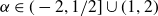
. The various contributions from [Reference Galkin and Galkina10,Reference Kahane15,Reference Mishura and Schied18,Reference Tabor and Tabor21] are illustrated in Figure 1, which shows the largest maximiser of the Takagi–Landsberg function
$\alpha\in(1,2)$
. The various contributions from [Reference Galkin and Galkina10,Reference Kahane15,Reference Mishura and Schied18,Reference Tabor and Tabor21] are illustrated in Figure 1, which shows the largest maximiser of the Takagi–Landsberg function $f_\alpha$
as a function of
$f_\alpha$
as a function of $\alpha$
. From Figure 1, it is apparent that the most interesting cases are
$\alpha$
. From Figure 1, it is apparent that the most interesting cases are $\alpha\in(-2,-1)$
and
$\alpha\in(-2,-1)$
and $\alpha\in(1/2,1]$
, which are also the ones about which nothing was known beyond the special parameters considered in [Reference Kahane15,Reference Tabor and Tabor21].
$\alpha\in(1/2,1]$
, which are also the ones about which nothing was known beyond the special parameters considered in [Reference Kahane15,Reference Tabor and Tabor21].

Fig. 1. Maximiser of $t\mapsto f_\alpha(t)$
in
$t\mapsto f_\alpha(t)$
in $[0,1/2]$
as a function of
$[0,1/2]$
as a function of $\alpha\in(-2,2)$
.
$\alpha\in(-2,2)$
.
In this paper, we present a completely new approach to the computation of the maximisers of the functions $f_\alpha$
. This approach works simultaneously for all parameters
$f_\alpha$
. This approach works simultaneously for all parameters $\alpha\in(-2,2)$
. It even extends to the entire Takagi class, which was introduced by Hata and Yamaguti [Reference Hata and Yamaguti14] and is formed by all functions of the form
$\alpha\in(-2,2)$
. It even extends to the entire Takagi class, which was introduced by Hata and Yamaguti [Reference Hata and Yamaguti14] and is formed by all functions of the form
 \begin{equation*}f(t):=\sum_{m=0}^\infty c_m\phi(2^mt),\qquad t\in[0,1],\end{equation*}
where $(c_m)_{m\in\mathbb N}$
is an absolutely summable sequence. An example is the choice
$(c_m)_{m\in\mathbb N}$
is an absolutely summable sequence. An example is the choice $c_m=2^{-m}\varepsilon_m$
, where
$c_m=2^{-m}\varepsilon_m$
, where $(\varepsilon_m)_{m\in\mathbb N}$
is an i.i.d. sequence of
$(\varepsilon_m)_{m\in\mathbb N}$
is an i.i.d. sequence of $\{-1,+1\}$
-valued Bernoulli random variables. For this example, the distribution of the maximum was studied by Allaart [Reference Allaart1]. Our approach works for arbitrary sequences
$\{-1,+1\}$
-valued Bernoulli random variables. For this example, the distribution of the maximum was studied by Allaart [Reference Allaart1]. Our approach works for arbitrary sequences $(c_m)_{m\in\mathbb N}$
and provides a recursive characterisation of the binary expansions of all maximisers and minimisers. This characterisation is called the step condition. It yields a simple method to compute the smallest and largest maximisers and minimisers of f with arbitrary precision. Moreover, it allows us to give exact statements on the cardinality of the set of maximisers and minimisers of f. For the case of the Takagi–Landsberg functions, we find that, for
$(c_m)_{m\in\mathbb N}$
and provides a recursive characterisation of the binary expansions of all maximisers and minimisers. This characterisation is called the step condition. It yields a simple method to compute the smallest and largest maximisers and minimisers of f with arbitrary precision. Moreover, it allows us to give exact statements on the cardinality of the set of maximisers and minimisers of f. For the case of the Takagi–Landsberg functions, we find that, for $\alpha\in(-2,-1)$
, the function
$\alpha\in(-2,-1)$
, the function $f_\alpha$
has either two or four maximisers, and we provide their exact values and the maximum values of
$f_\alpha$
has either two or four maximisers, and we provide their exact values and the maximum values of $f_\alpha$
in closed form. For
$f_\alpha$
in closed form. For $\alpha\in[-1,1/2]$
, the function
$\alpha\in[-1,1/2]$
, the function $f_\alpha$
has a unique maximiser at
$f_\alpha$
has a unique maximiser at $t=1/2$
, and for
$t=1/2$
, and for $\alpha\in(1,2)$
there are exactly two maximisers at
$\alpha\in(1,2)$
there are exactly two maximisers at $t=1/3$
and
$t=1/3$
and $t=2/3$
. The case
$t=2/3$
. The case $\alpha\in(1/2,1]$
is the most interesting. It will be discussed below.
$\alpha\in(1/2,1]$
is the most interesting. It will be discussed below.
In general, we show that non-uniqueness of maximisers in $[0,1/2]$
occurs if and only if there exists a Littlewood polynomial P for which the parameter
$[0,1/2]$
occurs if and only if there exists a Littlewood polynomial P for which the parameter $\alpha$
is a special root of P, called a step root. The step roots also coincide with the discontinuities of the functions that assign to each
$\alpha$
is a special root of P, called a step root. The step roots also coincide with the discontinuities of the functions that assign to each $\alpha\in(-2,2)$
the respective smallest and largest maximiser of
$\alpha\in(-2,2)$
the respective smallest and largest maximiser of $f_\alpha$
in
$f_\alpha$
in $[0,1/2]$
. We show that the polynomials
$[0,1/2]$
. We show that the polynomials $1-x-\cdots-x^{2n}$
are the only Littlewood polynomials with negative step roots, which in turn all belong to the interval
$1-x-\cdots-x^{2n}$
are the only Littlewood polynomials with negative step roots, which in turn all belong to the interval $(-2,-1)$
. They correspond exactly to the jumps in
$(-2,-1)$
. They correspond exactly to the jumps in $(-2,-1)$
of the function in Figure 1. While there are no step roots in
$(-2,-1)$
of the function in Figure 1. While there are no step roots in $[-1,1/2]\cup(1,2)$
, we show that the step roots lie dense in
$[-1,1/2]\cup(1,2)$
, we show that the step roots lie dense in $(1/2,1]$
. Moreover, if n is the smallest degree of a Littlewood polynomial that has
$(1/2,1]$
. Moreover, if n is the smallest degree of a Littlewood polynomial that has $\alpha\in(1/2,1]$
as a step root, then the set of maximisers of
$\alpha\in(1/2,1]$
as a step root, then the set of maximisers of $f_\alpha$
is a perfect set of Hausdorff dimension
$f_\alpha$
is a perfect set of Hausdorff dimension $1/(n+1)$
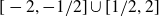
, and the binary expansions of all maximisers are given in explicit form in terms of the coefficients of the corresponding Littlewood polynomial. As a corollary, we show that the closure of the set of all real roots of all Littlewood polynomials is equal to
$1/(n+1)$
, and the binary expansions of all maximisers are given in explicit form in terms of the coefficients of the corresponding Littlewood polynomial. As a corollary, we show that the closure of the set of all real roots of all Littlewood polynomials is equal to $[-2,-1/2]\cup[1/2,2]$
.
$[-2,-1/2]\cup[1/2,2]$
.
This paper is organised as follows. In Section 2, we present general results for functions of the form (2 · 1). In Section 3, we discuss the particular case of the Takagi–Landsberg functions. The global maxima of $f_\alpha$
for the cases in which
$f_\alpha$
for the cases in which $\alpha$
belongs to the intervals
$\alpha$
belongs to the intervals $(-2,-1)$
,
$(-2,-1)$
, $[-1,1/2]$
,
$[-1,1/2]$
, $(1/2,1]$
, and (1,2) are analysed separately in the respective Subsections 3.1, 3.2, 3.3 and 3.4. We also discuss the global minima of
$(1/2,1]$
, and (1,2) are analysed separately in the respective Subsections 3.1, 3.2, 3.3 and 3.4. We also discuss the global minima of $f_\alpha$
in Subsection 3.5. As explained above, the maxima of the Takagi–Landsberg functions correspond to step roots of the Littlewood polynomials. Our results yield corollaries on the locations of such step roots and on the closure of the set of all real roots of the Littlewood polynomials. These corollaries are stated and proved in Section 4. The proofs of the results from Sections 2 and 3 are deferred to the respective Sections 5 and 6.
$f_\alpha$
in Subsection 3.5. As explained above, the maxima of the Takagi–Landsberg functions correspond to step roots of the Littlewood polynomials. Our results yield corollaries on the locations of such step roots and on the closure of the set of all real roots of the Littlewood polynomials. These corollaries are stated and proved in Section 4. The proofs of the results from Sections 2 and 3 are deferred to the respective Sections 5 and 6.
2. Maxima of functions in the Takagi class
The Takagi class was introduced in [Reference Hata and Yamaguti14]. It consists of the functions of the form
 \begin{equation}f(t):=\sum_{m=0}^\infty c_m\phi(2^mt),\qquad t\in[0,1],\end{equation}
where $\textbf{c}=(c_m)_{m\in\mathbb N}$
is a sequence in the space
$\textbf{c}=(c_m)_{m\in\mathbb N}$
is a sequence in the space $\ell^1$
of absolutely summable sequences and
$\ell^1$
of absolutely summable sequences and
 \begin{equation*}\phi(t):=\min_{z\in\mathbb Z}|t-z|,\qquad t\in{\mathbb R},\end{equation*}
is the tent map. Under this assumption, the series in (2 · 1) converges uniformly in t, so that f is a continuous function. The sequence $\textbf{c}\in\ell^1$
will be fixed throughout this section.
$\textbf{c}\in\ell^1$
will be fixed throughout this section.
For any $\{-1,+1\}$
-valued sequence
$\{-1,+1\}$
-valued sequence $\boldsymbol\rho=(\rho_m)_{m\in\mathbb N_0}$
, we let
$\boldsymbol\rho=(\rho_m)_{m\in\mathbb N_0}$
, we let
 \begin{equation}{ T}(\boldsymbol\rho)=\sum_{n=0}^\infty2^{-(n+2)}(1-\rho_n)\in[0,1].\end{equation}
Then $\varepsilon_n:=(1-\rho_n)/2$
will be the digits of a binary expansion of
$\varepsilon_n:=(1-\rho_n)/2$
will be the digits of a binary expansion of $t:={ T}(\boldsymbol\rho)$
. We will call
$t:={ T}(\boldsymbol\rho)$
. We will call $\boldsymbol\rho$
a Rademacher expansion of t. Clearly, the Rademacher expansion is unique unless t is a dyadic rational number in (0,1). Otherwise, t will admit two distinct Rademacher expansions. The one with infinitely many occurrences of the digit
$\boldsymbol\rho$
a Rademacher expansion of t. Clearly, the Rademacher expansion is unique unless t is a dyadic rational number in (0,1). Otherwise, t will admit two distinct Rademacher expansions. The one with infinitely many occurrences of the digit $+1$
will be called the standard Rademacher expansion. It can be obtained through the Rademacher functions, which are given by
$+1$
will be called the standard Rademacher expansion. It can be obtained through the Rademacher functions, which are given by $r_n(t):=(-1)^{\lfloor 2^{n+1} t\rfloor}$
. The following simple lemma illustrates the significance of the Rademacher expansion for the analysis of the function f.
$r_n(t):=(-1)^{\lfloor 2^{n+1} t\rfloor}$
. The following simple lemma illustrates the significance of the Rademacher expansion for the analysis of the function f.
Lemma 2.1. Let $\boldsymbol\rho=(\rho_m)_{m\in\mathbb N_0}$
be a Rademacher expansion of
$\boldsymbol\rho=(\rho_m)_{m\in\mathbb N_0}$
be a Rademacher expansion of $t\in[0,1]$
. Then
$t\in[0,1]$
. Then
 \begin{equation*}f(t)=\frac14\sum_{m=0}^\infty c_m\bigg(1-\sum_{k=1}^\infty 2^{-k}\rho_m\rho_{m+k}\bigg).\end{equation*}
The following concept is the key to our analysis of the maxima of the function f.
Definition 2.2. We will say that a $\{-1,+1\}$
-valued sequence
$\{-1,+1\}$
-valued sequence $(\rho_m)_{m\in\mathbb N_0}$
satisfies the step condition if
$(\rho_m)_{m\in\mathbb N_0}$
satisfies the step condition if
 \begin{equation*}\rho_{n}\sum_{m=0}^{n-1}2^mc_m\rho_m\le0\qquad\text{for all $n\in\mathbb N$.}\end{equation*}
Now we can state our first main result on the set of maximisers of f.
Theorem 2.3. For $t\in[0,1]$
, the following conditions are equivalent:
$t\in[0,1]$
, the following conditions are equivalent:
-
(a) t is a maximiser of f;
-
(b) every Rademacher expansion of t satisfies the step condition;
-
(c) there exists a Rademacher expansion of t that satisfies the step condition.
Theorem 2 · 3 provides a way to construct maximisers of f. More precisely, we define recursively the following pair of sequences $\boldsymbol\rho^{\flat}$
and
$\boldsymbol\rho^{\flat}$
and $\boldsymbol\rho^{\sharp}$
. We let
$\boldsymbol\rho^{\sharp}$
. We let $\rho^{\flat}_0=\rho^{\sharp}_0=1$
and, for
$\rho^{\flat}_0=\rho^{\sharp}_0=1$
and, for $n\in\mathbb N$
,
$n\in\mathbb N$
,
 \begin{equation}\rho_n^\flat=\begin{cases}+1&\text{if $\sum_{m=0}^{n-1}2^mc_m\rho^\flat_m<0$,}\\[3pt]-1&\text{otherwise,}\end{cases}\qquad \qquad\rho_n^\sharp=\begin{cases}+1&\text{if $\sum_{m=0}^{n-1}2^mc_m\rho^\sharp_m\le0$,}\\[3pt]-1&\text{otherwise.}\end{cases}\end{equation}
Corollary 2.4 With the above notation, ${ T}(\boldsymbol\rho^\flat)$
is the largest and
${ T}(\boldsymbol\rho^\flat)$
is the largest and ${ T}(\boldsymbol\rho^\sharp)$
is the smallest maximiser of f in
${ T}(\boldsymbol\rho^\sharp)$
is the smallest maximiser of f in $[0,1/2]$
.
$[0,1/2]$
.
Remark 2.5. By switching the signs in the sequence $(c_n)_{n\in\mathbb N_0}$
, we get analogous results for the minima of the function f. Specifically, if we define sequences
$(c_n)_{n\in\mathbb N_0}$
, we get analogous results for the minima of the function f. Specifically, if we define sequences $\boldsymbol\lambda^\flat$
and
$\boldsymbol\lambda^\flat$
and $\boldsymbol\lambda^\sharp$
by
$\boldsymbol\lambda^\sharp$
by $\lambda^\flat_0=\lambda^\sharp_0=+1$
and
$\lambda^\flat_0=\lambda^\sharp_0=+1$
and
 \begin{equation*}\lambda_n^\flat=\begin{cases}+1&\text{if $\sum_{m=0}^{n-1}2^mc_m\lambda^\flat_m>0$,}\\[3pt]-1&\text{otherwise,}\end{cases}\qquad \qquad\lambda_n^\sharp=\begin{cases}+1&\text{if $\sum_{m=0}^{n-1}2^mc_m\lambda^\sharp_m\ge0$,}\\[3pt]-1&\text{otherwise,}\end{cases}\end{equation*}
then ${ T}(\boldsymbol\lambda^\flat)$
is the largest and
${ T}(\boldsymbol\lambda^\flat)$
is the largest and ${ T}(\boldsymbol\lambda^\sharp)$
is the smallest minimiser of f in
${ T}(\boldsymbol\lambda^\sharp)$
is the smallest minimiser of f in $[0,1/2]$
.
$[0,1/2]$
.
The following corollary and its short proof illustrate the power of our method.
Corollary 2.6 We have $f(t)\ge0$
for all
$f(t)\ge0$
for all $t\in[0,1]$
, if and only if
$t\in[0,1]$
, if and only if $\sum_{m=0}^{n}2^mc_m\ge0$
for all
$\sum_{m=0}^{n}2^mc_m\ge0$
for all $n\ge0$
.
$n\ge0$
.
Proof. We have $f\ge0$
if and only if
$f\ge0$
if and only if $t=0$
is the smallest minimiser of f. By Remark2.5, this is equivalent to
$t=0$
is the smallest minimiser of f. By Remark2.5, this is equivalent to $\lambda_n^\sharp=+1$
for all n.
$\lambda_n^\sharp=+1$
for all n.
Our method also allows us to determine the cardinality of the set of maximisers of f. This is done in the following proposition.
Proposition 2.7 For $\boldsymbol\rho^\sharp$
as in (2 · 3), let
$\boldsymbol\rho^\sharp$
as in (2 · 3), let
 \begin{equation*}{\mathscr Z}:=\left\{n\in\mathbb N_0\,\Big|\,\sum_{m=0}^n2^mc_m\rho_m^\sharp=0\right\}.\end{equation*}
Then the number of $\{-1,+1\}$
-valued sequences
$\{-1,+1\}$
-valued sequences $\boldsymbol\rho$
that satisfy both the step condition and
$\boldsymbol\rho$
that satisfy both the step condition and $\rho_0=+1$
is
$\rho_0=+1$
is $2^{|{\mathscr Z}|}$
(where
$2^{|{\mathscr Z}|}$
(where $2^{\aleph_0}$
denotes as usual the cardinality of the continuum). In particular, the number of maximisers of f in
$2^{\aleph_0}$
denotes as usual the cardinality of the continuum). In particular, the number of maximisers of f in $[0,1/2]$
is equal to
$[0,1/2]$
is equal to $2^{|{\mathscr Z}|}$
, provided that all maximisers are not dyadic rationals.
$2^{|{\mathscr Z}|}$
, provided that all maximisers are not dyadic rationals.
Example 2.8. Consider the function f with $c_m=1/(m+1)^2$
, which was considered in [Reference Hata and Yamaguti14]. We claim that it has exactly two maximisers at
$c_m=1/(m+1)^2$
, which was considered in [Reference Hata and Yamaguti14]. We claim that it has exactly two maximisers at $t={11}/{24}$
and
$t={11}/{24}$
and $t={13}/{24}$
. See Figure 2 for an illustration. To prove our claim, we need to identify the sequence
$t={13}/{24}$
. See Figure 2 for an illustration. To prove our claim, we need to identify the sequence $\boldsymbol\rho^\sharp$
and show that the sums in (2 · 3) never vanish. A short computation yields that
$\boldsymbol\rho^\sharp$
and show that the sums in (2 · 3) never vanish. A short computation yields that $\rho^\sharp_0=1$
,
$\rho^\sharp_0=1$
, $\rho^\sharp_1=-1=\rho^\flat_1$
, and
$\rho^\sharp_1=-1=\rho^\flat_1$
, and $\rho^\sharp_2=-1=\rho^\flat_2$
. To simplify the notation, we let
$\rho^\sharp_2=-1=\rho^\flat_2$
. To simplify the notation, we let $\boldsymbol\rho:=\boldsymbol\rho^\sharp$
and define
$\boldsymbol\rho:=\boldsymbol\rho^\sharp$
and define
 \begin{equation*}R_n:=\sum_{m=0}^n\frac{2^m}{(m+1)^2}\rho_m.\end{equation*}
Next, we prove by induction on n that for $n\ge2$
,
$n\ge2$
,
 \begin{align}\rho_{2n-1}=-1\quad&\text{and}\quad \rho_{2n}=+1,\end{align}
 \begin{align} -\frac{2^{2n}}{(2n+1)^2} <R_{2n-1} < 0\quad&\text{and}\quad 0 < R_{2n}
< \frac{2^{2n+1}}{(2n+2)^2}.\end{align}
\begin{align} -\frac{2^{2n}}{(2n+1)^2} <R_{2n-1} < 0\quad&\text{and}\quad 0 < R_{2n}
< \frac{2^{2n+1}}{(2n+2)^2}.\end{align}
To establish the case $n=2$
, note first that
$n=2$
, note first that $R_2=1/{18}$
and hence
$R_2=1/{18}$
and hence $\rho_3=-1$
. It follows that
$\rho_3=-1$
. It follows that $R_3=1/18-8/16=-4/9$
. This gives in turn that
$R_3=1/18-8/16=-4/9$
. This gives in turn that $\rho_4=+1$
and
$\rho_4=+1$
and $R_4=-4/9+16/25=44/225$
. This establishes (2 · 4) and (2 · 5) for
$R_4=-4/9+16/25=44/225$
. This establishes (2 · 4) and (2 · 5) for $n=2$
. Now suppose that our claims have been established for all k with
$n=2$
. Now suppose that our claims have been established for all k with $2\le k\le n$
. Then the second inequality in (2 · 5) yields
$2\le k\le n$
. Then the second inequality in (2 · 5) yields $\rho_{2n+1}=-1$
and in turn
$\rho_{2n+1}=-1$
and in turn
 \begin{equation*}R_{2n+1}=R_{2n}-\frac{2^{2n+1}}{(2n+2)^2}>-\frac{2^{2n+1}}{(2n+2)^2}>-\frac{2^{2n+2}}{(2n+3)^2}\end{equation*}
and
 \begin{equation*}R_{2n+1}=R_{2n}-\frac{2^{2n+1}}{(2n+2)^2}<0.\end{equation*}
This yields $\rho_{2n+2}=+1$
, from which we get as above that
$\rho_{2n+2}=+1$
, from which we get as above that
 \begin{equation*}0<R_{2n+2}=R_{2n+1}+\frac{2^{2n+2}}{(2n+3)^2}<\frac{2^{2n+2}}{(2n+3)^2}<\frac{2^{2n+3}}{(2n+4)^2}.\end{equation*}
This proves our claims. Furthermore, (2 · 2) yields that the unique maximiser in $[0,1/2]$
is given by
$[0,1/2]$
is given by
 \begin{equation*}T(\boldsymbol\rho) = \frac{1}{4} + \frac{1}{8} + \frac{1}{16}\sum_{n = 0}^{\infty} \frac{1}{4^n} = \frac{11}{24}.\end{equation*}

Fig. 2. The function with $c_m=1/(m+1)^2$
analysed in Example 2 · 8. The vertical lines correspond to the two maxima at
$c_m=1/(m+1)^2$
analysed in Example 2 · 8. The vertical lines correspond to the two maxima at ${11}/{24}$
and at
${11}/{24}$
and at ${13}/{24}$
.
${13}/{24}$
.
3. Global extrema of the Takagi–Landsberg functions
The Takagi–Landsberg function with parameter $\alpha\in(-2,2)$
is given by
$\alpha\in(-2,2)$
is given by
 \begin{equation}f_\alpha(t):=\sum_{m=0}^\infty\frac{\alpha^m}{2^m}\phi(2^mt),\qquad t\in[0,1].\end{equation}
In the case $\alpha=1$
, the function
$\alpha=1$
, the function $f_1$
is the classical Takagi function, which was first introduced by Takagi [Reference Takagi22] and later rediscovered many times; see, e.g., the surveys [Reference Allaart and Kawamura2,Reference Lagarias16]. The class of functions
$f_1$
is the classical Takagi function, which was first introduced by Takagi [Reference Takagi22] and later rediscovered many times; see, e.g., the surveys [Reference Allaart and Kawamura2,Reference Lagarias16]. The class of functions $f_\alpha$
with
$f_\alpha$
with $-2<\alpha<2$
is sometimes also called the exponential Takagi class. See Figure 3 for an illustration.
$-2<\alpha<2$
is sometimes also called the exponential Takagi class. See Figure 3 for an illustration.

Fig. 3. Takagi–Landsberg functions $f_{-\alpha}$
(left) and
$f_{-\alpha}$
(left) and $f_\alpha$
(right) for four different values of
$f_\alpha$
(right) for four different values of $\alpha$
.
$\alpha$
.
By letting $c_m:=\alpha^m2^{-m}$
, we see that the results from Section 2 apply to the function
$c_m:=\alpha^m2^{-m}$
, we see that the results from Section 2 apply to the function $f_\alpha$
. In particular, Theorem 2 · 3 characterises the maximisers of
$f_\alpha$
. In particular, Theorem 2 · 3 characterises the maximisers of $f_\alpha$
in terms of a step condition satisfied by their Rademacher expansions. Let us restate the corresponding Definition 2 · 2 in our present situation.
$f_\alpha$
in terms of a step condition satisfied by their Rademacher expansions. Let us restate the corresponding Definition 2 · 2 in our present situation.
Definition 3.1. Let $\alpha\in(-2,2)$
. A
$\alpha\in(-2,2)$
. A $\{-1,+1\}$
-valued sequence
$\{-1,+1\}$
-valued sequence $(\rho_m)_{m\in\mathbb N_0}$
satisfies the step condition for
$(\rho_m)_{m\in\mathbb N_0}$
satisfies the step condition for $\alpha$
if
$\alpha$
if
 \begin{equation*}\rho_{n}\sum_{m=0}^{n-1}\alpha^m\rho_m\le0\qquad\text{for all $n\in\mathbb N$.}\end{equation*}
As in (2 · 3), we define recursively the following pair of sequences $\boldsymbol\rho^{\flat}(\alpha)$
and
$\boldsymbol\rho^{\flat}(\alpha)$
and $\boldsymbol\rho^{\sharp}(\alpha)$
. We let
$\boldsymbol\rho^{\sharp}(\alpha)$
. We let $\rho^{\flat}_0(\alpha)=\rho^{\sharp}_0(\alpha)=1$
and, for
$\rho^{\flat}_0(\alpha)=\rho^{\sharp}_0(\alpha)=1$
and, for $n\in\mathbb N$
,
$n\in\mathbb N$
,
 \begin{equation}\rho_n^\flat(\alpha)=\begin{cases}+1&\text{if $\sum_{m=0}^{n-1}\alpha^m\rho^\flat_m(\alpha)<0$,}\\[3pt]-1&\text{otherwise,}\end{cases}\qquad \qquad\rho_n^\sharp(\alpha)=\begin{cases}+1&\text{if $\sum_{m=0}^{n-1}\alpha^m\rho^\sharp_m(\alpha)\le0$,}\\[3pt]-1&\text{otherwise.}\end{cases}\end{equation}
Then we define
 \begin{equation*}\tau^\flat(\alpha):={ T}(\boldsymbol\rho^\flat(\alpha))\qquad \text{and}\qquad \tau^\sharp(\alpha):={ T}(\boldsymbol\rho^\sharp(\alpha)),\end{equation*}
where T is as in (2 · 2). It follows from Corollary 2 · 4 that $\tau^\flat(\alpha)$
is the largest and
$\tau^\flat(\alpha)$
is the largest and $\tau^\sharp(\alpha)$
is the smallest maximiser of
$\tau^\sharp(\alpha)$
is the smallest maximiser of $f_\alpha$
in
$f_\alpha$
in $[0,1/2]$
. We start with the following general result.
$[0,1/2]$
. We start with the following general result.
Proposition 3.2. For $\alpha\in(-2,2)$
, the following conditions are equivalent:
$\alpha\in(-2,2)$
, the following conditions are equivalent:
-
(a) The function $f_\alpha$
has a unique maximiser in
$[0,1/2]$
;
$f_\alpha$
has a unique maximiser in
$[0,1/2]$
; -
(b)
$\tau^\flat(\alpha)=\tau^\sharp(\alpha)$
; -
(c) There exists no
$n\in\mathbb N$
such that
$\sum_{m=0}^n\alpha^m\rho_m^\sharp(\alpha)=0$
; -
(d) The functions
$\tau^\flat$
and
$\tau^\sharp$
are continuous at
$\alpha$
.


In the following subsections, we discuss the maximization of $f_\alpha$
for various regimes of
$f_\alpha$
for various regimes of $\alpha$
.
$\alpha$
.
3.1 Global maxima for
$\alpha\in(-2,-1)$

To the best of our knowledge, the case $\alpha\in(-2,-1)$
has not yet been discussed in the literature. Here, we give an explicit solution for both maximisers and maximum values in this regime. Before stating our corresponding result, we formulate the following elementary lemma.
$\alpha\in(-2,-1)$
has not yet been discussed in the literature. Here, we give an explicit solution for both maximisers and maximum values in this regime. Before stating our corresponding result, we formulate the following elementary lemma.
Lemma 3.3. For $n\in\mathbb N$
, the Littlewood polynomial
$n\in\mathbb N$
, the Littlewood polynomial $p_{2n}(x)=1-x-\cdots-x^{2n-1}-x^{2n}$
has a unique negative root
$p_{2n}(x)=1-x-\cdots-x^{2n-1}-x^{2n}$
has a unique negative root $x_{n}$
. Moreover, the sequence
$x_{n}$
. Moreover, the sequence $(x_{n})_{n\in\mathbb N}$
is strictly increasing, belongs to
$(x_{n})_{n\in\mathbb N}$
is strictly increasing, belongs to $(-2,-1)$
, and converges to
$(-2,-1)$
, and converges to $-1$
as
$-1$
as $n\uparrow\infty$
.
$n\uparrow\infty$
.
Note that $-x_1= (1+\sqrt5)/2\approx 1.61803$
is the golden ratio. Approximate numerical values for the next highest roots are
$-x_1= (1+\sqrt5)/2\approx 1.61803$
is the golden ratio. Approximate numerical values for the next highest roots are $x_2\approx -1.29065$
,
$x_2\approx -1.29065$
, $x_3\approx -1.19004$
,
$x_3\approx -1.19004$
, $x_4\approx -1.14118$
, and
$x_4\approx -1.14118$
, and $x_5\approx -1.11231$
.
$x_5\approx -1.11231$
.
Theorem 3.4. Let $(x_{n})_{n\in\mathbb N_0}$
be the sequence introduced in Lemma 3 · 3 with
$(x_{n})_{n\in\mathbb N_0}$
be the sequence introduced in Lemma 3 · 3 with $x_0:=-2$
. Then, for
$x_0:=-2$
. Then, for $\alpha \in (x_n,x_{n+1})$
, the function
$\alpha \in (x_n,x_{n+1})$
, the function $f_\alpha$
has exactly two maximisers in [0,1], which are located at
$f_\alpha$
has exactly two maximisers in [0,1], which are located at
 \begin{equation*}t_n:=\frac1{10}(5-4^{-n})\quad\text{and}\quad 1-t_n=\frac1{10}(5+4^{-n}).\end{equation*}
If $\alpha=x_n$
for some
$\alpha=x_n$
for some $n\in\mathbb N$
, then
$n\in\mathbb N$
, then $f_\alpha$
has exactly four maximisers in [0,1], which are located at
$f_\alpha$
has exactly four maximisers in [0,1], which are located at $t_{n-1}$
,
$t_{n-1}$
, $t_{n}$
,
$t_{n}$
, $1-t_{n-1}$
and
$1-t_{n-1}$
and $1-t_{n}$
. Moreover,
$1-t_{n}$
. Moreover,
 \begin{equation}f_\alpha(t_n)=\frac{1}{10} (5-4^{-n})-\frac{4^{-n}}{10} \cdot\frac{ 3 \alpha^{2 n+3}+ \alpha^3-4 \alpha}{(1-\alpha) \left(\alpha^2-4\right)},\end{equation}
and this is equal to the maximum value of $f_\alpha$
if
$f_\alpha$
if $\alpha\in[x_n,x_{n+1}]$
.
$\alpha\in[x_n,x_{n+1}]$
.
Remark 3.5. It is easy to see that the right-hand side of (3 · 3) is strictly larger than $1/2$
for
$1/2$
for $\alpha\in(-2,-1)$
. Moreover, it tends to
$\alpha\in(-2,-1)$
. Moreover, it tends to $+\infty$
for
$+\infty$
for $\alpha\downarrow-2$
and to
$\alpha\downarrow-2$
and to $1/2$
for
$1/2$
for $\alpha\uparrow-1$
.
$\alpha\uparrow-1$
.
3.2 Global maxima for
$\alpha\in[-1,1/2]$

Galkin and Galkina [Reference Galkin and Galkina10] proved that for $\alpha\in[-1,1/2]$
the function
$\alpha\in[-1,1/2]$
the function $f_\alpha$
has a global maximum at
$f_\alpha$
has a global maximum at $t=1/2$
with maximum value
$t=1/2$
with maximum value $f_\alpha(1/2)=1/2$
. Here, we give a short proof of this result by using our method and additionally establish the uniqueness of the maximiser.
$f_\alpha(1/2)=1/2$
. Here, we give a short proof of this result by using our method and additionally establish the uniqueness of the maximiser.
Proposition 3.6. For $\alpha\in[-1,1/2]$
, the function
$\alpha\in[-1,1/2]$
, the function $f_\alpha$
has the unique maximiser
$f_\alpha$
has the unique maximiser $t=1/2$
and the maximum value
$t=1/2$
and the maximum value $f_\alpha(1/2)=1/2$
.
$f_\alpha(1/2)=1/2$
.
Proof. Since obviously $f_\alpha(1/2)=1/2$
for all
$f_\alpha(1/2)=1/2$
for all $\alpha$
, the result will follow if we can establish that
$\alpha$
, the result will follow if we can establish that $\tau^\sharp(\alpha)=1/2$
for all
$\tau^\sharp(\alpha)=1/2$
for all $\alpha\in[-1,1/2]$
. This is the case if
$\alpha\in[-1,1/2]$
. This is the case if $\boldsymbol\rho:=\boldsymbol\rho^\sharp(\alpha)$
satisfies
$\boldsymbol\rho:=\boldsymbol\rho^\sharp(\alpha)$
satisfies $\rho_n=-1$
for all
$\rho_n=-1$
for all $n\ge1$
. We prove this by induction on n. The case
$n\ge1$
. We prove this by induction on n. The case $n=1$
follows immediately from
$n=1$
follows immediately from $\rho_0=1$
and (3 · 2). If
$\rho_0=1$
and (3 · 2). If $\rho_1=\cdots=\rho_{n-1}=-1$
has already been established, then
$\rho_1=\cdots=\rho_{n-1}=-1$
has already been established, then
 \begin{equation*}\sum_{m=0}^{n-1}\alpha^m\rho_m=\frac{\alpha^n-2\alpha+1}{1-\alpha}.\end{equation*}
If the right-hand side is strictly positive, then we have $\rho_n=-1$
. Positivity is obvious for
$\rho_n=-1$
. Positivity is obvious for $\alpha\in[-1,0]$
and for
$\alpha\in[-1,0]$
and for $\alpha=1/2$
. For
$\alpha=1/2$
. For $\alpha\in(0,1/2)$
, we can take the derivative of the numerator with respect to
$\alpha\in(0,1/2)$
, we can take the derivative of the numerator with respect to $\alpha$
. This derivative is equal to
$\alpha$
. This derivative is equal to $n\alpha^{n-1}-2$
, which is strictly negative for
$n\alpha^{n-1}-2$
, which is strictly negative for $\alpha\in(0,1/2)$
, because
$\alpha\in(0,1/2)$
, because $n\alpha^{n-1}\le1$
for those
$n\alpha^{n-1}\le1$
for those $\alpha$
. Since the numerator is strictly positive for
$\alpha$
. Since the numerator is strictly positive for $\alpha=1/2$
, the result follows.
$\alpha=1/2$
, the result follows.
3.3. Global maxima for
$\alpha\in(1/2,1]$

This is the most interesting regime, as can already be seen from Figure 1. Kahane [Reference Kahane15] showed that the maximum value of the classical Takagi function $f_1$
is
$f_1$
is $2/3$
and that the set of maximisers is equal to the set of all points in [0,Reference Allaart1] whose binary expansion satisfies
$2/3$
and that the set of maximisers is equal to the set of all points in [0,Reference Allaart1] whose binary expansion satisfies $\varepsilon_{2n}+\varepsilon_{2n+1}=1$
for each
$\varepsilon_{2n}+\varepsilon_{2n+1}=1$
for each $n\in\mathbb N_0$
. This is a perfect set of Hausdorff dimension
$n\in\mathbb N_0$
. This is a perfect set of Hausdorff dimension $1/2$
. For other values of
$1/2$
. For other values of $\alpha\in(1/2,1]$
, we are only aware of the following result by Tabor and Tabor [Reference Tabor and Tabor21]. They found the maximum value of
$\alpha\in(1/2,1]$
, we are only aware of the following result by Tabor and Tabor [Reference Tabor and Tabor21]. They found the maximum value of $f_{\alpha_n}$
, where
$f_{\alpha_n}$
, where $\alpha_n$
is the unique positive root of the Littlewood polynomial
$\alpha_n$
is the unique positive root of the Littlewood polynomial $1-x-x^2-\cdots -x^n$
. This sequence satisfies
$1-x-x^2-\cdots -x^n$
. This sequence satisfies $\alpha_1=1$
and
$\alpha_1=1$
and $\alpha_n\downarrow1/2$
as
$\alpha_n\downarrow1/2$
as $n\uparrow\infty$
. The maximum value of
$n\uparrow\infty$
. The maximum value of $f_{\alpha_n}$
is then given by
$f_{\alpha_n}$
is then given by $C(\alpha_n)$
, where
$C(\alpha_n)$
, where
 \begin{equation}C(\alpha):=\frac{1}{2-2(2 \alpha -1)^{\frac{\log_2 \alpha-1}{\log_2 \alpha }}}.\end{equation}
Tabor and Tabor [Reference Tabor and Tabor21] observed numerically that the maximum value of $f_\alpha$
typically differs from
$f_\alpha$
typically differs from $C(\alpha)$
for other values of
$C(\alpha)$
for other values of $\alpha\in(1/2,1)$
. In Example 3 · 11 we will investigate a specific choice of
$\alpha\in(1/2,1)$
. In Example 3 · 11 we will investigate a specific choice of $\alpha$
for which
$\alpha$
for which $C(\alpha)$
is indeed different from the maximum value of
$C(\alpha)$
is indeed different from the maximum value of $f_\alpha$
. In Example3.10, we will characterise the set of maximisers of
$f_\alpha$
. In Example3.10, we will characterise the set of maximisers of $f_{\alpha_n}$
, where
$f_{\alpha_n}$
, where $\alpha_n$
is as above.
$\alpha_n$
is as above.
We have seen in Sections 3.1 and 3.2 that for $\alpha\le1/2$
the function
$\alpha\le1/2$
the function $f_\alpha$
has either two or four maximisers in [0,Reference Allaart1]. For
$f_\alpha$
has either two or four maximisers in [0,Reference Allaart1]. For $\alpha>1/2$
this situation changes. The following result shows that then
$\alpha>1/2$
this situation changes. The following result shows that then $f_\alpha$
will have either two or uncountably many maximisers. Moreover, the result quoted in Section 3.4 will imply that the latter case can only happen for
$f_\alpha$
will have either two or uncountably many maximisers. Moreover, the result quoted in Section 3.4 will imply that the latter case can only happen for $\alpha\in(1/2,1]$
.
$\alpha\in(1/2,1]$
.
Theorem 3.7. For $\alpha>1/2$
, we have the following dichotomy:
$\alpha>1/2$
, we have the following dichotomy:
-
(a) if
$\sum_{m=0}^n\alpha^m\rho^\sharp_m\neq0$
for all n, then the function
$f_\alpha$
has exactly two maximisers in [0,1]. They are given by
$\tau^\sharp(\alpha)$
and
$1-\tau^\sharp(\alpha)$
and have
$\boldsymbol\rho^\sharp$
and
$-\boldsymbol\rho^\sharp$
as their Rademacher expansions; -
(b) otherwise, let
$n_0$
be the smallest n such that
$\sum_{m=0}^n\alpha^m\rho^\sharp_m=0$
. Then the set of maximisers of
$f_\alpha$
consists of all those
$t\in[0,1]$
that have a Rademacher expansion consisting of successive blocks of the form
$\rho^\sharp_0,\dots, \rho^\sharp_{n_0}$
or
$(-\rho^\sharp_0),\dots,(- \rho^\sharp_{n_0})$
. This is a perfect set of Hausdorff dimension
$1/(n_0+1)$
and its
$1/(n_0+1)$
-Hausdorff measure is finite and strictly positive.


The preceding theorem yields the following corollary.
Corollary 3.8 For $\alpha>1/2$
, the function
$\alpha>1/2$
, the function $f_\alpha$
cannot have a maximiser that is a dyadic rational number.
$f_\alpha$
cannot have a maximiser that is a dyadic rational number.
Note that Theorem 3 · 4 implies that also for $\alpha<-1$
there are no dyadic rational maximisers. However, by Proposition 3 · 6, the unique maximiser in case
$\alpha<-1$
there are no dyadic rational maximisers. However, by Proposition 3 · 6, the unique maximiser in case $-1\le \alpha\le1/2$
is
$-1\le \alpha\le1/2$
is $t=1/2$
.
$t=1/2$
.
Our next result shows in particular that there is no nonempty open interval in $(1/2,1]$
on which
$(1/2,1]$
on which $\tau^\flat$
or
$\tau^\flat$
or $\tau^\sharp$
are constant.
$\tau^\sharp$
are constant.
Theorem 3.9. There is no nonempty open interval in $(1/2,1)$
on which the functions
$(1/2,1)$
on which the functions $\tau^\flat$
or
$\tau^\flat$
or $\tau^\sharp$
are continuous.
$\tau^\sharp$
are continuous.
Example 3.10. Tabor and Tabor [Reference Tabor and Tabor21] found the maximum value of $f_{\alpha_n}$
, where
$f_{\alpha_n}$
, where $\alpha_n$
is the unique positive root of the Littlewood polynomial
$\alpha_n$
is the unique positive root of the Littlewood polynomial $1-x-x^2-\cdots -x^n$
. The case
$1-x-x^2-\cdots -x^n$
. The case $n=1$
, and in turn
$n=1$
, and in turn $\alpha_1=1$
, corresponds to the classical Takagi function as studied by Kahane [Reference Kahane15]. Here, we will now determine the corresponding sets of maximisers. It is clear that we must have
$\alpha_1=1$
, corresponds to the classical Takagi function as studied by Kahane [Reference Kahane15]. Here, we will now determine the corresponding sets of maximisers. It is clear that we must have $1-\sum_{k=1}^m\alpha_n^k>0$
for
$1-\sum_{k=1}^m\alpha_n^k>0$
for $m=1,\dots, n-1$
. Hence,
$m=1,\dots, n-1$
. Hence,
 \begin{align*}\boldsymbol\rho^\sharp(\alpha_n)&=(+1,\underbrace{-1,\dots,-1}_{\text{n times}},+1,\underbrace{-1,\dots,-1}_{\text{n times}},\dots),\\\boldsymbol\rho^\flat(\alpha_n)&=(+1,\underbrace{-1,\dots,-1}_{\text{n times}},-1,\underbrace{+1,\dots,+1}_{\text{n times}},-1,\underbrace{+1,\dots,+1}_{\text{n times}},\dots).\end{align*}
Every maximiser in [0,1] has a Rademacher expansion that is made up of successive blocks of length $n+1$
taking the form
$n+1$
taking the form $+1,-1,\dots,-1$
or
$+1,-1,\dots,-1$
or $-1,+1\dots, +1$
. This is a perfect set of Hausdorff dimension
$-1,+1\dots, +1$
. This is a perfect set of Hausdorff dimension $1/(n+1)$
. The smallest maximiser is given by
$1/(n+1)$
. The smallest maximiser is given by
 \begin{align*}\tau^\sharp(\alpha_n)&=\sum_{m=0}^\infty\sum_{k=2}^{n+1}2^{-(m(n+1)+k)}=\Big(\frac12-2^{-(n+1)}\Big)\sum_{m=0}^\infty2^{-m(n+1)}=\frac{2^n-1}{2^{n+1}-1}.\end{align*}
The largest maximiser in $[0,1/2]$
is
$[0,1/2]$
is
 \begin{equation*}\tau^\flat(\alpha_n)=\frac12-2^{-(n+1)}+\sum_{m=1}^\infty 2^{-m(n+1)-1}=\frac{1}{2} \Big(1-2^{-n}+\frac{1}{2^{n+1}-1}\Big).\end{equation*}
Example 3.11. Consider the choice
 \begin{equation*}\alpha=\frac14\Big(1+\sqrt{13}-\sqrt{2\big(\sqrt{13}-1\big)}\Big)\approx 0.580692.\end{equation*}
One checks that $1-\alpha-\alpha^2-\alpha^3+\alpha^4=0$
and that
$1-\alpha-\alpha^2-\alpha^3+\alpha^4=0$
and that $1-\alpha-\alpha^2-\alpha^3<0$
and
$1-\alpha-\alpha^2-\alpha^3<0$
and $1-\alpha-\alpha^2>0$
and
$1-\alpha-\alpha^2>0$
and $1-\alpha>0$
. Therefore,
$1-\alpha>0$
. Therefore,
 \begin{align*}\boldsymbol\rho^\sharp(\alpha)&=(+1,-1,-1,-1,+1,+1,-1,-1,-1,+1,+1,-1,-1,-1,+1,\dots)\\\boldsymbol\rho^\flat(\alpha)&=(+1,-1,-1,-1,+1,-1,+1,+1,+1,-1,-1,+1,+1,+1,-1,\dots),\end{align*}
and every maximiser in [0,1] has a Rademacher expansion that consists of successive blocks of the form $+1,-1,-1,-1,+1$
or
$+1,-1,-1,-1,+1$
or $-1,+1,+1,+1,-1$
. This is a Cantor-type set of Hausdorff dimension
$-1,+1,+1,+1,-1$
. This is a Cantor-type set of Hausdorff dimension $1/5$
. Furthermore,
$1/5$
. Furthermore,
 \begin{align*}\tau^\sharp(\alpha)&=\sum_{n=0}^\infty\big(0\cdot 2^{-(5n+1)}+2^{-(5n+2)}+ 2^{-(5n+3)}+ 2^{-(5n+4)}+0\cdot 2^{-(5n+5)}\big)=\frac{14}{31}\approx 0.451613\end{align*}
is the smallest maximiser, and
 \begin{equation*}\tau^\flat(\alpha)=\frac7{16}+\sum_{n=1}^\infty \big(2^{-5n-1}+2^{-5n-5}\big)=\frac{451}{992}\approx 0.454637\end{equation*}
is the largest maximiser in $[0,1/2]$
. To compute the maximum value, we can either use Lemma 2 · 1, or we directly compute
$[0,1/2]$
. To compute the maximum value, we can either use Lemma 2 · 1, or we directly compute $f_\alpha(14/31)$
as follows. We note that
$f_\alpha(14/31)$
as follows. We note that $\phi(2^{5n+k}14/31)=b_k/31$
, where
$\phi(2^{5n+k}14/31)=b_k/31$
, where $b_0=14$
,
$b_0=14$
, $b_1=3$
,
$b_1=3$
, $b_2=6$
,
$b_2=6$
, $b_3=12$
, and
$b_3=12$
, and $b_4=7$
. Thus,
$b_4=7$
. Thus,
 \begin{align*}f_\alpha(14/31)&=\frac1{31}\sum_{n=0}^\infty\Big(\frac\alpha2\Big)^{5n}\Big(14+3\frac\alpha2+6\Big(\frac\alpha2\Big)^2+12\Big(\frac\alpha2\Big)^3+7\Big(\frac\alpha2\Big)^4\Big)\\[3pt]&=\frac{39+3 \sqrt{13}-\sqrt{6 \left(25+7 \sqrt{13}\right)}}{56-2\sqrt{13}+4 \sqrt{7+2 \sqrt{13}}}\approx 0.508155,\end{align*}
where the second identity was obtained by using Mathematica 12.0. For the function in (3 · 4), we get, however, $C(\alpha)\approx 0.508008$
, which confirms the numerical observation from [Reference Tabor and Tabor21] that
$C(\alpha)\approx 0.508008$
, which confirms the numerical observation from [Reference Tabor and Tabor21] that $C(\cdot)$
may not yield correct maximum values if evaluated at arguments different from the positive roots of
$C(\cdot)$
may not yield correct maximum values if evaluated at arguments different from the positive roots of $1-x-x^2-\cdots -x^n$
.
$1-x-x^2-\cdots -x^n$
.
3.4. Global maxima for
$\alpha\in(1,2)$

For $\alpha=\sqrt2$
, it can be deduced from [11, lemma 5] that
$\alpha=\sqrt2$
, it can be deduced from [11, lemma 5] that $f_{\sqrt2}$
has maxima at
$f_{\sqrt2}$
has maxima at $t=1/3$
and
$t=1/3$
and $t=2/3$
and maximum value
$t=2/3$
and maximum value $(2+\sqrt2)/3$
. That lemma was later rediscovered by the second author in [20, lemma 3
$(2+\sqrt2)/3$
. That lemma was later rediscovered by the second author in [20, lemma 3 $\cdot$
1]. The statement on the maxima of
$\cdot$
1]. The statement on the maxima of $f_{\sqrt2}$
was given independently in [Reference Galkin and Galkina10,Reference Schied20]. Mishura and Schied [Reference Mishura and Schied18] extended this subsequently to the following result, which we quote here for the sake of completeness. It is not difficult to prove it with our present method; see [13, example 4
$f_{\sqrt2}$
was given independently in [Reference Galkin and Galkina10,Reference Schied20]. Mishura and Schied [Reference Mishura and Schied18] extended this subsequently to the following result, which we quote here for the sake of completeness. It is not difficult to prove it with our present method; see [13, example 4 $\cdot$
3
$\cdot$
3 $\cdot$
1].
$\cdot$
1].
Theorem 3.12. (Mishura and Schied [Reference Mishura and Schied18]) For $\alpha\in(1,2)$
, the function
$\alpha\in(1,2)$
, the function $f_\alpha$
has exactly two maximisers at
$f_\alpha$
has exactly two maximisers at $t=1/3$
and
$t=1/3$
and $t=2/3$
and its maximum value is
$t=2/3$
and its maximum value is $(3(1-\alpha/2))^{-1}$
.
$(3(1-\alpha/2))^{-1}$
.
3.5. Global minima
In this section, we discuss the minima of the function $f_\alpha$
.
$f_\alpha$
.
Theorem 3.13. for the global minima of the function $f_\alpha$
, we have the following three cases.
$f_\alpha$
, we have the following three cases.
-
(a) for
$\alpha\in(-2,-1)$
, the function
$f_\alpha$
has a unique minimum in
$[0,1/2]$
, which is located at
$t=1/5$
. Moreover, the minimum value is
\begin{equation*}f_\alpha(1/5)=\frac{1+\alpha}{5(1-(\alpha/2)^2)}.\end{equation*}
-
(b) for
$\alpha=-1$
, the minimum value of
$f_\alpha$
is equal to 0, and the set of minimisers is equal to the set of all
$t\in[0,1]$
that have a Rademacher expansion
$\boldsymbol\rho$
with
$\rho_{2n}=\rho_{2n+1}$
for
$n\in\mathbb N_0$
. This is a perfect set of Hausdorff dimension
$1/2$
, and its
$1/2$
-dimensional Hausdorff measure is finite and strictly positive. -
(c) for
$\alpha\in(-1,2)$
, the unique minimiser of
$f_\alpha$
in
$[0,1/2]$
is at
$t=0$
and the minimum value is
$f_\alpha(0)=0$
.


The preceding theorem and Remark 3.5 yield immediately the following corollary.
Corollary 3.14 The function $f_\alpha(t)$
is nonnegative for all
$f_\alpha(t)$
is nonnegative for all $t\in[0,1]$
if and only if
$t\in[0,1]$
if and only if $\alpha\ge-1$
. Moreover, there is no
$\alpha\ge-1$
. Moreover, there is no $\alpha\in(-2,2)$
such that
$\alpha\in(-2,2)$
such that $f_\alpha$
is nonpositive.
$f_\alpha$
is nonpositive.
The fact that $f_\alpha\ge0$
for
$f_\alpha\ge0$
for $\alpha\ge-1$
can alternatively be deduced from an argument in the proof of [10, Theorem 4.1].
$\alpha\ge-1$
can alternatively be deduced from an argument in the proof of [10, Theorem 4.1].
4. Real (step) roots of Littlewood polynomials
In this section, we link our analysis of the maxima of the Takagi–Landsberg functions to certain real roots of the Littlewood polynomials. Recall that a Littlewood polynomial is a polynomial whose coefficients are all $-1$
or
$-1$
or $+1$
. By [4, corollary 3
$+1$
. By [4, corollary 3 $\cdot$
3
$\cdot$
3 $\cdot$
1], the complex roots of any Littlewood polynomial must lie in the annulus
$\cdot$
1], the complex roots of any Littlewood polynomial must lie in the annulus $\{z\in\mathbb C\,|\,1/2<|z|<2\}$
. Hence, the real roots can only lie in
$\{z\in\mathbb C\,|\,1/2<|z|<2\}$
. Hence, the real roots can only lie in $(-2,-1/2)\cup(1/2,2)$
. Below, we will show in Corollary 4.5 that the real roots are actually dense in that set. We start with the following simple lemma.
$(-2,-1/2)\cup(1/2,2)$
. Below, we will show in Corollary 4.5 that the real roots are actually dense in that set. We start with the following simple lemma.
Lemma 4.1. The numbers $-1$
and
$-1$
and $+1$
are the only rational roots for Littlewood polynomials.
$+1$
are the only rational roots for Littlewood polynomials.
Proof. Assume $\alpha \in \mathbb{Q}$
is a rational root for some Littlewood polynomial
$\alpha \in \mathbb{Q}$
is a rational root for some Littlewood polynomial $P_n(x)$
. Then the monic polynomial
$P_n(x)$
. Then the monic polynomial $x - \alpha$
divides
$x - \alpha$
divides $P_n(x)$
. The Gauss lemma yields that
$P_n(x)$
. The Gauss lemma yields that $x - \alpha \in \mathbb{Z}[x]$
and hence
$x - \alpha \in \mathbb{Z}[x]$
and hence $\alpha \in \mathbb{Z}$
. By the above-mentioned [4, corollary 3
$\alpha \in \mathbb{Z}$
. By the above-mentioned [4, corollary 3 $\cdot$
3
$\cdot$
3 $\cdot$
1], we get
$\cdot$
1], we get $|\alpha| = 1$
.
$|\alpha| = 1$
.
Definition 4.2. For given $n\in\mathbb N$
, let
$n\in\mathbb N$
, let $P_n(x)=\sum_{m=0}^n\rho_mx^m$
be a Littlewood polynomial with coefficients
$P_n(x)=\sum_{m=0}^n\rho_mx^m$
be a Littlewood polynomial with coefficients $\rho_m\in\{-1,+1\}$
. If
$\rho_m\in\{-1,+1\}$
. If $k\le n$
, we write
$k\le n$
, we write $P_k(x)=\sum_{m=0}^k\rho_mx^m$
. A number
$P_k(x)=\sum_{m=0}^k\rho_mx^m$
. A number $\alpha\in{\mathbb R}$
is called a step root of
$\alpha\in{\mathbb R}$
is called a step root of $P_n$
if
$P_n$
if $P_n(\alpha)=0$
and
$P_n(\alpha)=0$
and $\rho_{k+1}P_k(\alpha)\le0$
for
$\rho_{k+1}P_k(\alpha)\le0$
for $k=0,\dots, n-1$
.
$k=0,\dots, n-1$
.
The concept of a step root has the following significance for the maxima of the Takagi–Landsberg functions $f_\alpha$
defined in (3 · 1).
$f_\alpha$
defined in (3 · 1).
Corollary 4.3 For $\alpha\in(-2,2)$
, the following conditions are equivalent:
$\alpha\in(-2,2)$
, the following conditions are equivalent:
-
(a) the function
$f_\alpha$
has a unique maximiser in
$[0,1/2]$
. -
(b) there is no Littlewood polynomial that has
$\alpha$
as its step root.


Proof. The assertion follows immediately from Proposition 3.2 and Theorem 2 · 3.
With our results on the maxima of the Takagi–Landsberg function, we thus get the following corollary on the locations of the step roots of the Littlewood polynomials.
Corollary 4.4. We have the following results:
-
(a) the only Littlewood polynomials admitting negative step roots are of the form
$1-x-x^2-\cdots-x^{2n}$
for some
$n\in\mathbb N$
and the step roots are the numbers
$x_n$
in Lemma 3 · 3
-
(b) there are no step roots in
$[-1,1/2]\cup(1,2)$
-
(c) the step roots are dense in
$(1/2,1]$
.


Proof. In view of Corollary 4 · 3, (a) follows from Theorem 3 · 4. Assertion (b) follows from Proposition 3 · 6 and Theorem 3 · 12. Part (c) follows from Theorem3.9.
From part (c) of the preceding corollary, we obtain the following result, which identifies $[-2,-1/2]\cup[1/2,2]$
as the closure of the set of all real roots of the Littlewood polynomials. Although the roots of the Littlewood polynomials have been well studied in the literature (see, e.g, [Reference Borwein5] and the references therein), we were unable to find the following result in the literature. In [5, E1 on p. 72], it is stated that an analogous result holds if the Littlewood polynomials are replaced by the larger set of all polynomials with coefficients in
$[-2,-1/2]\cup[1/2,2]$
as the closure of the set of all real roots of the Littlewood polynomials. Although the roots of the Littlewood polynomials have been well studied in the literature (see, e.g, [Reference Borwein5] and the references therein), we were unable to find the following result in the literature. In [5, E1 on p. 72], it is stated that an analogous result holds if the Littlewood polynomials are replaced by the larger set of all polynomials with coefficients in $\{-1,0,+1\}$
. In the student thesis [Reference Vader23], determining the closure of the real roots of the Littlewood polynomials was classified as an open problem. The distribution of the positive roots and step roots of Littlewood polynomials is illustrated in Figure 4.
$\{-1,0,+1\}$
. In the student thesis [Reference Vader23], determining the closure of the real roots of the Littlewood polynomials was classified as an open problem. The distribution of the positive roots and step roots of Littlewood polynomials is illustrated in Figure 4.

Fig. 4. Log-scale histograms of the distributions of the positive roots (left) and step roots (right) of the Littlewood polynomials of degree $\le 20$
and with zero-order coefficient
$\le 20$
and with zero-order coefficient $\rho_0=+1$
. The algorithm found 2,255,683 roots and 106,682 step roots, where numbers such as
$\rho_0=+1$
. The algorithm found 2,255,683 roots and 106,682 step roots, where numbers such as $\alpha=1$
were counted each time they occurred as (step) roots of some polynomial.
$\alpha=1$
were counted each time they occurred as (step) roots of some polynomial.
Corollary 4.5 Let ${\mathscr R}$
denote the set of all real roots of the Littlewood polynomials. Then the closure of
${\mathscr R}$
denote the set of all real roots of the Littlewood polynomials. Then the closure of ${\mathscr R}$
is given by
${\mathscr R}$
is given by $[-2,-1/2]\cup[1/2,2]$
.
$[-2,-1/2]\cup[1/2,2]$
.
Proof. We know from [4, corollary 3 $\cdot$
3
$\cdot$
3 $\cdot$
1] that
$\cdot$
1] that ${\mathscr R}\subset(-2,-1/2)\cup(1/2,2)$
. Now denote by
${\mathscr R}\subset(-2,-1/2)\cup(1/2,2)$
. Now denote by ${\mathscr S}$
the set of all step roots of the Littlewood polynomials, so that
${\mathscr S}$
the set of all step roots of the Littlewood polynomials, so that ${\mathscr S}\subset{\mathscr R}$
. Corollary 4.4 (c) yields that
${\mathscr S}\subset{\mathscr R}$
. Corollary 4.4 (c) yields that $[1/2,1]$
is contained in the closure of
$[1/2,1]$
is contained in the closure of ${\mathscr S}$
, and hence also in the closure of
${\mathscr S}$
, and hence also in the closure of ${\mathscr R}$
. Next, note that if
${\mathscr R}$
. Next, note that if $\alpha$
is the root of a Littlewood polynomial, then so is
$\alpha$
is the root of a Littlewood polynomial, then so is $1/\alpha$
. Indeed, if
$1/\alpha$
. Indeed, if $\alpha$
is a root of the Littlewood polynomial P(x), then
$\alpha$
is a root of the Littlewood polynomial P(x), then $\widetilde P(x):=x^nP(1/x)$
is also a Littlewood polynomial and satisfies
$\widetilde P(x):=x^nP(1/x)$
is also a Littlewood polynomial and satisfies $\widetilde P(1/\alpha)=\alpha^{-n}P(\alpha)=0$
. Hence, [Reference Allaart1,Reference Allaart and Kawamura2] is contained in the closure of
$\widetilde P(1/\alpha)=\alpha^{-n}P(\alpha)=0$
. Hence, [Reference Allaart1,Reference Allaart and Kawamura2] is contained in the closure of ${\mathscr R}$
. Finally, for
${\mathscr R}$
. Finally, for $\alpha\in{\mathscr R}$
, we clearly have also
$\alpha\in{\mathscr R}$
, we clearly have also $-\alpha\in{\mathscr R}$
. This completes the proof.
$-\alpha\in{\mathscr R}$
. This completes the proof.
5. Proofs of the results in Section 2
Proof of Lemma 2 · 1. Take $m\in\mathbb N_0$
and let
$m\in\mathbb N_0$
and let $t\in[0,1]$
have Rademacher expansion
$t\in[0,1]$
have Rademacher expansion $\boldsymbol\rho$
. Then the tent map satisfies
$\boldsymbol\rho$
. Then the tent map satisfies
 \begin{equation*}\phi(t)=\frac14-\frac14\sum_{k=1}^\infty 2^{-k}\rho_0\rho_k\quad\text{and}\quad \phi(2^mt)=\frac14-\frac14\sum_{k=1}^\infty 2^{-k}\rho_m\rho_{m+k}.\end{equation*}
Plugging this formula into (2 · 1) gives the result.
By
 \begin{equation*}f_{n}(t):=\sum_{m=0}^n c_m\phi(2^mt),\qquad t\in[0,1],\end{equation*}
we will denote the corresponding truncated function.
Let
 \begin{equation*}{\mathbb D}_n:=\{k2^{-n}\,|\,k=0,\dots,2^n\}\end{equation*}
be the dyadic partition of [0,1] of generation n. For $t\in{\mathbb D}_n$
, we define its set of neighbours in
$t\in{\mathbb D}_n$
, we define its set of neighbours in ${\mathbb D}_n$
by
${\mathbb D}_n$
by
 \begin{equation*}{\mathscr N}_n(t)=\{s\in{\mathbb D}_n\,|\,|t-s|=2^{-n}\}.\end{equation*}
If $s\in{\mathscr N}_n(t)$
, we will say that s and t are neighbouring points in
$s\in{\mathscr N}_n(t)$
, we will say that s and t are neighbouring points in ${\mathbb D}_n$
. We are now going to analyse the maxima of the truncated function
${\mathbb D}_n$
. We are now going to analyse the maxima of the truncated function $f_{n}$
. Since this function is affine on all intervals of the form
$f_{n}$
. Since this function is affine on all intervals of the form $[k2^{-(n+1)},(k+1)2^{-(n+1)}]$
, it is clear that its maximum must be attained on
$[k2^{-(n+1)},(k+1)2^{-(n+1)}]$
, it is clear that its maximum must be attained on ${\mathbb D}_{n+1}$
. In addition,
${\mathbb D}_{n+1}$
. In addition, $f_n$
can have flat parts (e.g.,
$f_n$
can have flat parts (e.g., $n=0$
and
$n=0$
and $c_0=0$
), so that the set of maximisers of
$c_0=0$
), so that the set of maximisers of $f_n$
may be an uncountable set. In the sequel, we are only interested in the set
$f_n$
may be an uncountable set. In the sequel, we are only interested in the set
 \begin{equation*}{\mathscr M}_n={\mathbb D}_{n+1}\cap\mathop{\rm{arg }}{\mkern 1mu} {\rm{max}}{f_n}\end{equation*}
of maximisers located in ${\mathbb D}_{n+1}$
.
${\mathbb D}_{n+1}$
.
Definition 5.1. For $n\in\mathbb N_0$
, a pair
$n\in\mathbb N_0$
, a pair $(x_n,y_n)$
is called a maximising edge of generation n if the following conditions are satisfied:
$(x_n,y_n)$
is called a maximising edge of generation n if the following conditions are satisfied:
-
(a)
$x_n\in{\mathscr M}_n$
; -
(b)
$y_n$
is a maximiser of
$f_n$
in
${\mathscr N}_{n+1}(x_n)$
, i.e.,
$${y_n} \in \mathop {{\rm{arg }}{\mkern 1mu} {\rm{max}}}\limits_{x \in {{\mathscr N}_{n + 1}}({x_n})} {f_n}(x)$$
.


The following lemma characterises the maximising edges of generation n as the maximisers of $f_n$
over neighbouring pairs in
$f_n$
over neighbouring pairs in ${\mathbb D}_{n+1}$
. It will be a key result for our proof of Theorem 2 · 3.
${\mathbb D}_{n+1}$
. It will be a key result for our proof of Theorem 2 · 3.
Lemma 5.2. For $n\in\mathbb N_0$
, the following conditions are equivalent for two neighboring points
$n\in\mathbb N_0$
, the following conditions are equivalent for two neighboring points $x_n,\,y_n\in{\mathbb D}_{n+1}$
:
$x_n,\,y_n\in{\mathbb D}_{n+1}$
:
-
(a)
$(x_n,y_n)$
or
$(y_n,x_n)$
is a maximising edge of generation n; -
(b) for all neighboring points
$z_0,z_1$
in
${\mathbb D}_{n+1}$
, we have
$f_n(z_0)+f_n(z_1)\le f_n(x_n)+f_n(y_n)$
.


Proof. We prove the assertion by induction on n. Consider the case $n=0$
. If
$n=0$
. If $c_0=0$
, then
$c_0=0$
, then ${\mathscr M}_0={\mathbb D}_1$
and all pairs of neighbouring points in
${\mathscr M}_0={\mathbb D}_1$
and all pairs of neighbouring points in ${\mathbb D}_1$
form maximising edges of generation 0, and so the assertion is obvious. If
${\mathbb D}_1$
form maximising edges of generation 0, and so the assertion is obvious. If $c_0>0$
, then
$c_0>0$
, then ${\mathscr M}_0=\{1/2\}$
, and if
${\mathscr M}_0=\{1/2\}$
, and if $c_0<0$
, then
$c_0<0$
, then ${\mathscr M}_0=\{0,1\}$
. Also in these cases the equivalence of (a) and (b) is obvious.ow assume that
${\mathscr M}_0=\{0,1\}$
. Also in these cases the equivalence of (a) and (b) is obvious.ow assume that $n\ge1$
and that the equivalence of (a) and (b) has been established for all
$n\ge1$
and that the equivalence of (a) and (b) has been established for all $m<n$
. To show that (a) implies (b), let
$m<n$
. To show that (a) implies (b), let $(x_n,y_n)$
be a maximising edge of generation n. First, we consider the case
$(x_n,y_n)$
be a maximising edge of generation n. First, we consider the case $x_n\in{\mathbb D}_{n+1}\setminus{\mathbb D}_n$
. Then
$x_n\in{\mathbb D}_{n+1}\setminus{\mathbb D}_n$
. Then ${\mathscr N}_{n+1}(x_n)$
contains
${\mathscr N}_{n+1}(x_n)$
contains $y_n$
and another point, say
$y_n$
and another point, say $u_n$
, and both
$u_n$
, and both $y_n$
and
$y_n$
and $u_n$
belong to
$u_n$
belong to ${\mathbb D}_n$
. If
${\mathbb D}_n$
. If $z_0$
and
$z_0$
and $z_2$
are two neighbouring points in
$z_2$
are two neighbouring points in ${\mathbb D}_n$
, we let
${\mathbb D}_n$
, we let $z_1:=(z_0+z_2)/2$
. Then
$z_1:=(z_0+z_2)/2$
. Then
 \begin{equation*}\frac12\big(f_{n-1}(z_0)+f_{n-1}(z_2)\big)+\frac{c_n}2=f_n(z_1)\le f_n(x_n)=\frac12\big(f_{n-1}(y_n)+f_{n-1}(u_n)\big)+\frac{c_n}2,\end{equation*}
and hence $f_{n-1}(z_0)+f_{n-1}(z_2)\le f_{n-1}(y_n)+f_{n-1}(u_n)$
. The induction hypothesis now yields that
$f_{n-1}(z_0)+f_{n-1}(z_2)\le f_{n-1}(y_n)+f_{n-1}(u_n)$
. The induction hypothesis now yields that $(y_n,u_n)$
or
$(y_n,u_n)$
or $(u_n,y_n)$
is a maximising edge of generation
$(u_n,y_n)$
is a maximising edge of generation $n-1$
. Moreover, since
$n-1$
. Moreover, since $(x_n,y_n)$
is a maximising edge of generation n, part (b) of Definition 5.1 gives
$(x_n,y_n)$
is a maximising edge of generation n, part (b) of Definition 5.1 gives $f_n(u_n)\le f_n(y_n)$
. Since both
$f_n(u_n)\le f_n(y_n)$
. Since both $y_n$
and
$y_n$
and $u_n$
belong to
$u_n$
belong to ${\mathbb D}_n$
, we get that
${\mathbb D}_n$
, we get that
 \begin{equation}f_{n-1}(u_n)=f_n(u_n)\le f_n(y_n)=f_{n-1}(y_n).\end{equation}
Therefore, $y_n\in{\mathscr M}_{n-1}$
.
$y_n\in{\mathscr M}_{n-1}$
.
Now let $z_0$
and
$z_0$
and $z_1$
be two neighboring points in
$z_1$
be two neighboring points in ${\mathbb D}_{n+1}$
. Then one of the two, say
${\mathbb D}_{n+1}$
. Then one of the two, say $z_0$
belongs to
$z_0$
belongs to ${\mathbb D}_n$
. Hence, the fact that
${\mathbb D}_n$
. Hence, the fact that $y_n\in{\mathscr M}_{n-1}$
and
$y_n\in{\mathscr M}_{n-1}$
and $x_n\in{\mathscr M}_n$
yields that
$x_n\in{\mathscr M}_n$
yields that
 \begin{equation*}f_n(z_0)+f_n(z_1)=f_{n-1}(z_0)+f_n(z_1)\le f_{n-1}(y_n)+f_n(x_n)= f_{n}(y_n)+f_n(x_n). \end{equation*}
This establishes (b) in case $x_n\in{\mathbb D}_{n+1}\setminus{\mathbb D}_n$
.
$x_n\in{\mathbb D}_{n+1}\setminus{\mathbb D}_n$
.
Now we consider the case in which $x_n\in{\mathbb D}_n$
. Then
$x_n\in{\mathbb D}_n$
. Then $f_{n-1}(x_n)=f_n(x_n)$
, and so
$f_{n-1}(x_n)=f_n(x_n)$
, and so $x_n\in{\mathscr M}_{n-1}$
. Next, we let
$x_n\in{\mathscr M}_{n-1}$
. Next, we let $y_{n-1}:=2y_n-x_n$
. Then
$y_{n-1}:=2y_n-x_n$
. Then $y_{n-1}\in{\mathbb D}_{n}$
, and we claim that
$y_{n-1}\in{\mathbb D}_{n}$
, and we claim that $(x_n,y_{n-1})$
is a maximising edge of generation
$(x_n,y_{n-1})$
is a maximising edge of generation $n-1$
. This is obvious if
$n-1$
. This is obvious if $x_n\in\{0,1\}$
. Otherwise, we have
$x_n\in\{0,1\}$
. Otherwise, we have ${\mathscr N}_{n}(x_n)=\{y_{n-1},u_{n-1}\}$
for
${\mathscr N}_{n}(x_n)=\{y_{n-1},u_{n-1}\}$
for $u_{n-1}=2x_n-y_{n-1}=3x_n-2y_n$
. Moreover,
$u_{n-1}=2x_n-y_{n-1}=3x_n-2y_n$
. Moreover, ${\mathscr N}_{n+1}(x_n)=\{y_n,u_n\}$
for
${\mathscr N}_{n+1}(x_n)=\{y_n,u_n\}$
for $u_n=\frac12(x_n+u_{n-1})$
. Since
$u_n=\frac12(x_n+u_{n-1})$
. Since $(x_n,y_n)$
is a maximising edge of generation n, we must have
$(x_n,y_n)$
is a maximising edge of generation n, we must have $ f_n(y_n)\ge f_n(u_n)$
and hence
$ f_n(y_n)\ge f_n(u_n)$
and hence
 \begin{align*}\frac12\big(f_{n-1}(x_n)+f_{n-1}(y_{n-1})\big)+\frac{c_n}2=f_n(y_n)\ge f_n(u_n)=\frac12\big(f_{n-1}(x_n)+f_{n-1}(u_{n-1})\big)+\frac{c_n}2. \end{align*}
Therefore,
 \begin{equation} f_{n-1}( y_{n-1})\ge f_{n-1}(u_{n-1}), \end{equation}
and it follows that $(x_n,y_{n-1})$
is indeed a maximising edge of generation
$(x_n,y_{n-1})$
is indeed a maximising edge of generation $n-1$
.
$n-1$
.
Now let $z_0$
and
$z_0$
and $z_1$
be two neighbouring points in
$z_1$
be two neighbouring points in ${\mathbb D}_{n+1}$
. Exactly one of these points, say
${\mathbb D}_{n+1}$
. Exactly one of these points, say $z_0$
, belongs also to
$z_0$
, belongs also to ${\mathbb D}_n$
. Let
${\mathbb D}_n$
. Let $z_2:=2z_1-z_0\in{\mathbb D}_n$
, so that
$z_2:=2z_1-z_0\in{\mathbb D}_n$
, so that $z_0$
and
$z_0$
and $z_2$
are neighbouring points in
$z_2$
are neighbouring points in ${\mathbb D}_n$
and
${\mathbb D}_n$
and $z_1=(z_0+z_2)/2$
. Hence,
$z_1=(z_0+z_2)/2$
. Hence, $f_n(z_1)=\big(f_{n-1}(z_0)+f_{n-1}(z_2)\big)/2+{c_n}/2$
. Therefore, the fact that
$f_n(z_1)=\big(f_{n-1}(z_0)+f_{n-1}(z_2)\big)/2+{c_n}/2$
. Therefore, the fact that $ f_n(z_0)\le f_n(x_n)$
and the induction hypothesis yield that
$ f_n(z_0)\le f_n(x_n)$
and the induction hypothesis yield that
 \begin{align*}f_n(z_0)+f_n(z_1)&\le f_n(x_n)+ \frac12\big(f_{n-1}(x_{n})+f_{n-1}(y_{n-1})\big)+\frac{c_n}2= f_n(x_n)+ f_n(y_n).\end{align*}
This completes the proof of (a) $\Rightarrow$
(b).
$\Rightarrow$
(b).
Now we prove (b) $\Rightarrow$
(a). To this end, let
$\Rightarrow$
(a). To this end, let $x_n$
and
$x_n$
and $y_n$
be two fixed neighboring points in
$y_n$
be two fixed neighboring points in ${\mathbb D}_{n+1}$
such that (b) is satisfied. Without loss of generality, we may suppose that
${\mathbb D}_{n+1}$
such that (b) is satisfied. Without loss of generality, we may suppose that $f_n(x_n)\ge f_n(y_n)$
. Clearly,
$f_n(x_n)\ge f_n(y_n)$
. Clearly, $y_n$
must be a maximiser of
$y_n$
must be a maximiser of $f_n$
in
$f_n$
in ${\mathscr N}_{n+1}(x_n)$
. To conclude (a), it will thus be sufficient to show that
${\mathscr N}_{n+1}(x_n)$
. To conclude (a), it will thus be sufficient to show that $x_n\in{\mathscr M}_n$
. To this end, we first consider the case
$x_n\in{\mathscr M}_n$
. To this end, we first consider the case $x_n\in{\mathbb D}_n$
. In a first step, we claim that
$x_n\in{\mathbb D}_n$
. In a first step, we claim that $x_n\in{\mathscr M}_{n-1}$
. To this end, we assume by way of contradiction that there is
$x_n\in{\mathscr M}_{n-1}$
. To this end, we assume by way of contradiction that there is $z_0\in{\mathscr M}_{n-1}$
such that
$z_0\in{\mathscr M}_{n-1}$
such that $f_{n-1}(z_0)>f_{n-1}(x_n)=f_n(x_n)$
. Then we take
$f_{n-1}(z_0)>f_{n-1}(x_n)=f_n(x_n)$
. Then we take $z_2\in{\mathbb D}_n$
such that
$z_2\in{\mathbb D}_n$
such that $(z_0,z_2)$
is a maximising edge of generation
$(z_0,z_2)$
is a maximising edge of generation $n-1$
and define
$n-1$
and define $z_1:=(z_0+z_2)/2$
and
$z_1:=(z_0+z_2)/2$
and $y_{n-1}:=2y_n-x_n\in{\mathbb D}_n$
. Using our assumption (b) yields that
$y_{n-1}:=2y_n-x_n\in{\mathbb D}_n$
. Using our assumption (b) yields that
 \begin{align*}&{f_{n-1}(x_n)+\frac12\big(f_{n-1}(x_n)+f_{n-1}(y_{n-1})\big)+\frac{c_n}2}\\[3pt]&=f_n(x_n)+f_n(y_n)\ge f_n(z_0)+f_n(z_1)\\[3pt]&=f_{n-1}(z_0)+\frac12\big(f_{n-1}(z_0)+f_{n-1}(z_2)\big)+\frac{c_n}2\\[3pt]&>f_{n-1}(x_n)+\frac12\big(f_{n-1}(z_0)+f_{n-1}(z_2)\big)+\frac{c_n}2.\end{align*}
Hence, $f_{n-1}(x_n)+f_{n-1}(y_{n-1})>f_{n-1}(z_0)+f_{n-1}(z_2)$
, in contradiction to our assumption that
$f_{n-1}(x_n)+f_{n-1}(y_{n-1})>f_{n-1}(z_0)+f_{n-1}(z_2)$
, in contradiction to our assumption that $(z_0,z_2)$
is a maximising edge of generation
$(z_0,z_2)$
is a maximising edge of generation $n-1$
and the induction hypothesis. Therefore we must have
$n-1$
and the induction hypothesis. Therefore we must have $x_n\in{\mathscr M}_{n-1}$
.
$x_n\in{\mathscr M}_{n-1}$
.
In the next step, we show that $f_n(x_n)\ge f_n(z)$
for all
$f_n(x_n)\ge f_n(z)$
for all $z\in{\mathbb D}_{n+1}\setminus{\mathbb D}_n$
. Together with the preceding step, this will give
$z\in{\mathbb D}_{n+1}\setminus{\mathbb D}_n$
. Together with the preceding step, this will give $x_n\in{\mathscr M}_n$
. To this end, let
$x_n\in{\mathscr M}_n$
. To this end, let $z_1\in{\mathbb D}_{n+1}\setminus{\mathbb D}_n$
be given, and let
$z_1\in{\mathbb D}_{n+1}\setminus{\mathbb D}_n$
be given, and let $z_0$
and
$z_0$
and $z_2$
be the two neighbors of
$z_2$
be the two neighbors of $z_1$
in
$z_1$
in ${\mathbb D}_{n+1}$
. Then
${\mathbb D}_{n+1}$
. Then $z_0,z_2\in{\mathbb D}_n$
and
$z_0,z_2\in{\mathbb D}_n$
and $z_1=\frac12(z_0+z_2)$
. As discussed above,
$z_1=\frac12(z_0+z_2)$
. As discussed above, $y_n$
is a maximiser of
$y_n$
is a maximiser of $f_n$
in
$f_n$
in ${\mathscr N}_{n+1}(x_n)$
. Thus, it is easy to see that
${\mathscr N}_{n+1}(x_n)$
. Thus, it is easy to see that $y_{n-1}:=2y_n-x_n$
must be a maximiser of
$y_{n-1}:=2y_n-x_n$
must be a maximiser of $f_{n-1}$
in
$f_{n-1}$
in ${\mathscr N}_{n}(x_n)$
. Since we already know that
${\mathscr N}_{n}(x_n)$
. Since we already know that $x_n\in{\mathscr M}_{n-1}$
, the induction hypothesis yields that
$x_n\in{\mathscr M}_{n-1}$
, the induction hypothesis yields that $(x_n,y_{n-1})$
is a maximising edge of generation
$(x_n,y_{n-1})$
is a maximising edge of generation $n-1$
. Thus,
$n-1$
. Thus,
 \begin{align*}f_n(z_1)&=\frac12\big(f_{n-1}(z_0)+f_{n-1}(z_2)\big)+\frac{c_n}2\le \frac12\big(f_{n-1}(x_n)+f_{n-1}(y_{n-1})\big)+\frac{c_n}2\\&=f_n(y_n)\le f_n(x_n).\end{align*}
This concludes the proof of (b) $\Rightarrow$
(a) in case
$\Rightarrow$
(a) in case $x_n\in{\mathbb D}_n$
.
$x_n\in{\mathbb D}_n$
.
Now we consider the case in which $x_n\in{\mathbb D}_{n+1}\setminus{\mathbb D}_n$
. In a first step, we show that
$x_n\in{\mathbb D}_{n+1}\setminus{\mathbb D}_n$
. In a first step, we show that $y_n\in{\mathscr M}_{n-1}$
. To this end, we assume by way of contradiction that there is
$y_n\in{\mathscr M}_{n-1}$
. To this end, we assume by way of contradiction that there is $z_0\in{\mathscr M}_{n-1}$
such that
$z_0\in{\mathscr M}_{n-1}$
such that $f_{n-1}(z_0)>f_{n-1}(y_n)$
. Let
$f_{n-1}(z_0)>f_{n-1}(y_n)$
. Let $z_2\in{\mathbb D}_n$
be such that
$z_2\in{\mathbb D}_n$
be such that $(z_0,z_2)$
is a maximising edge of generation
$(z_0,z_2)$
is a maximising edge of generation $n-1$
and put
$n-1$
and put $z_1:=(z_0+z_2)/2$
. We also put
$z_1:=(z_0+z_2)/2$
. We also put $u_n:=2x_n-y_n$
. Then the induction hypothesis gives
$u_n:=2x_n-y_n$
. Then the induction hypothesis gives
 \begin{align*}f_n(z_0)+f_n(z_1)&=f_{n-1}(z_0)+\frac12\big(f_{n-1}(z_0)+f_{n-1}(z_2)\big)+\frac{c_n}2\\&>f_{n-1}(y_n)+\frac12\big(f_{n-1}(y_n)+f_{n-1}(u_n)\big)+\frac{c_n}2\\&=f_n(y_n)+f_n(x_n),\end{align*}
in contradiction to our assumption (b). Thus, $y_n\in{\mathscr M}_{n-1}$
.
$y_n\in{\mathscr M}_{n-1}$
.
Next, we show that $(y_n,u_n)$
is a maximising edge of generation
$(y_n,u_n)$
is a maximising edge of generation $n-1$
. This is clear if either
$n-1$
. This is clear if either $y_n$
or
$y_n$
or $u_n$
belong to
$u_n$
belong to $\{0,1\}$
. Otherwise, we must show that
$\{0,1\}$
. Otherwise, we must show that $f_{n-1}(u_n)\ge f_{n-1}(w_n)$
, where
$f_{n-1}(u_n)\ge f_{n-1}(w_n)$
, where $w_n=2y_n-u_n$
. Let
$w_n=2y_n-u_n$
. Let $z_n:=(w_n+y_n)/2$
. Then our hypothesis (b) yields that
$z_n:=(w_n+y_n)/2$
. Then our hypothesis (b) yields that $f_n(y_n)+f_n(x_n)\ge f_n(y_n)+f_n(z_n)$
and in turn
$f_n(y_n)+f_n(x_n)\ge f_n(y_n)+f_n(z_n)$
and in turn $f_n(x_n)\ge f_n(z_n)$
. It follows that
$f_n(x_n)\ge f_n(z_n)$
. It follows that
 \begin{align*}\frac12\big(f_{n-1}(y_n)+f_{n-1}(u_n)\big)+\frac{c_n}2=f_n(x_n)\ge f_n(z_n)=\frac12\big(f_{n-1}(y_n)+f_{n-1}(w_n)\big)+\frac{c_n}2,\end{align*}
which implies the desired inequality $f_{n-1}(u_n)\ge f_{n-1}(w_n)$
.
$f_{n-1}(u_n)\ge f_{n-1}(w_n)$
.
Now we can conclude our proof by showing that $x_n\in{\mathscr M}_n$
. If
$x_n\in{\mathscr M}_n$
. If $z\in{\mathbb D}_n$
, then the fact that
$z\in{\mathbb D}_n$
, then the fact that $y_n\in{\mathscr M}_{n-1}$
gives
$y_n\in{\mathscr M}_{n-1}$
gives
 \begin{equation*}f_n(x_n)\ge f_n(y_n)=f_{n-1}(y_n)\ge f_{n-1}(z)=f_n(z).\end{equation*}
If $z\in{\mathbb D}_{n+1}\setminus{\mathbb D}_n$
, we let
$z\in{\mathbb D}_{n+1}\setminus{\mathbb D}_n$
, we let $z_0$
and
$z_0$
and $z_2$
denote its two neighbouring points in
$z_2$
denote its two neighbouring points in ${\mathbb D}_{n+1}$
, so that
${\mathbb D}_{n+1}$
, so that $z_0,z_2\in{\mathbb D}_n$
and
$z_0,z_2\in{\mathbb D}_n$
and $z=(z_0+z_2)/2$
. Then,
$z=(z_0+z_2)/2$
. Then,
 \begin{equation*}f_n(z)=\frac12\big(f_{n-1}(z_0)+f_{n-1}(z_2)\big)+\frac{c_n}2\le \frac12\big(f_{n-1}(y_n)+f_{n-1}(u_n)\big)+\frac{c_n}2=f_n(x_n),\end{equation*}
where we have used the induction hypothesis and the fact that $(y_n,u_n)$
is a maximising edge of generation
$(y_n,u_n)$
is a maximising edge of generation $n-1$
.
$n-1$
.
In the proof of the preceding lemma (see, in particular, (5 · 1) and (5 · 2)), we have en passant proved the following statement, which shows how to successively construct maximising edges in a backward manner.
Lemma 5.3. Suppose that $(x_n,y_n)$
is a maximising edge of generation
$(x_n,y_n)$
is a maximising edge of generation $n\ge1$
. Then:
$n\ge1$
. Then:
-
(a) if
$x_n\in{\mathbb D}_n$
and
$y_{n-1}:=2y_n-x_n$
, then
$(x_n,y_{n-1})$
is a maximising edge of generation
$n-1$
. -
(b) if
$x_n\in{\mathbb D}_{n+1}\setminus{\mathbb D}_n$
and
$u_n:=2x_n-y_n$
, then
$(y_n,u_n)$
is a maximising edge of generation
$n-1$
.


We also have the following result, which shows how maximising edges can be constructed in a forward manner.
Lemma 5.4. For $n\in\mathbb N_0$
let
$n\in\mathbb N_0$
let $(x_n,y_n)$
be a maximising edge of generation n and define
$(x_n,y_n)$
be a maximising edge of generation n and define $z_n:=(x_n+y_n)/2$
. Then
$z_n:=(x_n+y_n)/2$
. Then $(x_n,z_n)$
or
$(x_n,z_n)$
or $(z_n,x_n)$
is a maximising edge of generation
$(z_n,x_n)$
is a maximising edge of generation $n+1$
.
$n+1$
.
Proof. Note that $f_{n+1}(z_n)=(f_n(x_n)+f_n(y_n))+c_{n+1}/2$
. Hence, property (b) in Lemma 5.2 yields that
$f_{n+1}(z_n)=(f_n(x_n)+f_n(y_n))+c_{n+1}/2$
. Hence, property (b) in Lemma 5.2 yields that $f_{n+1}(z_n)\ge f_{n+1}(z)$
for all
$f_{n+1}(z_n)\ge f_{n+1}(z)$
for all $z\in{\mathbb D}_{n+2}\setminus{\mathbb D}_{n+1}$
. Moreover, by assumption,
$z\in{\mathbb D}_{n+2}\setminus{\mathbb D}_{n+1}$
. Moreover, by assumption, $f_{n+1}(x_n)=f_n(x_n)\ge f_n(z)=f_{n+1}(z)$
for all
$f_{n+1}(x_n)=f_n(x_n)\ge f_n(z)=f_{n+1}(z)$
for all $z\in{\mathbb D}_{n+1}$
. Hence,
$z\in{\mathbb D}_{n+1}$
. Hence, $z_n\in{\mathscr M}_{n+1}$
if
$z_n\in{\mathscr M}_{n+1}$
if $f_{n+1}(z_n) \ge f_{n+1}(x_n)$
and
$f_{n+1}(z_n) \ge f_{n+1}(x_n)$
and $x_n\in{\mathscr M}_{n+1}$
if
$x_n\in{\mathscr M}_{n+1}$
if $f_{n+1}(x_n) \ge f_{n+1}(z_n)$
. From here, the assertion follows easily.
$f_{n+1}(x_n) \ge f_{n+1}(z_n)$
. From here, the assertion follows easily.
The next proposition states in particular, that t is a maximiser of f if and only if it is a limit of successive maximisers of $f_n$
. Clearly, the “if” direction of this statement is obvious, while the only if” direction is not.
$f_n$
. Clearly, the “if” direction of this statement is obvious, while the only if” direction is not.
Proposition 5.5. For given $t\in[0,1]$
, the following statements are equivalent.
$t\in[0,1]$
, the following statements are equivalent.
-
(a)
$t\in\mathop \rm{arg} \,max f$
. -
(b) there exists a sequence
$(t_n)_{n\in\mathbb N_0}$
such that
$t_n\in{\mathscr M}_n$
for all n and
$\lim_nt_n=t$
. -
(c) for
$n\in\mathbb N_0$
, let
$E_n$
be the union of all intervals [x,y] such that
$x,y\in{\mathbb D}_{n+1}$
,
$x<y$
and (x,y) or (y,x) is a maximising edge of generation n. Then
\begin{equation*}t\in\bigcap_{n=0}^\infty E_n.\end{equation*}


Proof. To prove (a) $\Rightarrow$
(c), we assume by way of contradiction that there is
$\Rightarrow$
(c), we assume by way of contradiction that there is $n\in\mathbb N_0$
such that
$n\in\mathbb N_0$
such that $t\notin E_n$
. Clearly, we can take the smallest such n. Since
$t\notin E_n$
. Clearly, we can take the smallest such n. Since $E_0=[0,1]$
, we must have
$E_0=[0,1]$
, we must have $n\ge1$
. Moreover, there must be a maximising edge of generation
$n\ge1$
. Moreover, there must be a maximising edge of generation $n-1$
, denoted
$n-1$
, denoted $(x_{n-1},y_{n-1})$
, such that t belongs to the closed interval with endpoints
$(x_{n-1},y_{n-1})$
, such that t belongs to the closed interval with endpoints $x_{n-1}$
and
$x_{n-1}$
and $y_{n-1}$
. Let
$y_{n-1}$
. Let $z:=(x_{n-1}+y_{n-1})/2$
. By Lemma5.4, the closed interval with endpoints
$z:=(x_{n-1}+y_{n-1})/2$
. By Lemma5.4, the closed interval with endpoints $x_{n-1}$
and z is a subset of
$x_{n-1}$
and z is a subset of $E_n$
. Hence,
$E_n$
. Hence, $t\neq z$
and t must be contained in the half-open interval with endpoints z and
$t\neq z$
and t must be contained in the half-open interval with endpoints z and $y_{n-1}$
. Therefore,
$y_{n-1}$
. Therefore, $t=\alpha y_{n-1}+(1-\alpha)z$
for some
$t=\alpha y_{n-1}+(1-\alpha)z$
for some $\alpha\in(0,1]$
. We define
$\alpha\in(0,1]$
. We define $s:=\alpha x_{n-1}+(1-\alpha)z=2z -t$
.
$s:=\alpha x_{n-1}+(1-\alpha)z=2z -t$
.
Since the interval with endpoints z and $y_{n-1}$
is not a subset of
$y_{n-1}$
is not a subset of $E_n$
, Lemma 5.2 implies that
$E_n$
, Lemma 5.2 implies that $f_n(z)+f_n(y_{n-1})<f_n(z)+f_n(x_{n-1})$
. As
$f_n(z)+f_n(y_{n-1})<f_n(z)+f_n(x_{n-1})$
. As $f_n$
is affine on each of the two respective intervals with endpoints
$f_n$
is affine on each of the two respective intervals with endpoints $y_{n-1}, z$
and
$y_{n-1}, z$
and $z,x_{n-1}$
, we thus get
$z,x_{n-1}$
, we thus get $f_n(s)>f_n(t)$
. Moreover, the symmetry and periodicity of the tent map
$f_n(s)>f_n(t)$
. Moreover, the symmetry and periodicity of the tent map $\phi$
implies that
$\phi$
implies that $\phi(2^mt)=\phi(2^ms)$
for all
$\phi(2^mt)=\phi(2^ms)$
for all $m> n$
. Hence,
$m> n$
. Hence,
 \begin{equation*}f(s)=f_n(s)+\sum_{m=n+1}^\infty c_m\phi(2^ms)>f_n( t)+\sum_{m=n+1}^\infty c_m\phi(2^m t)=f(t),\end{equation*}
which contradicts the assumed maximality of t.
The implication (c) $\Rightarrow$
(b) is obvious, because
$\Rightarrow$
(b) is obvious, because $|x_n-y_n|=2^{-(n+1)}$
whenever
$|x_n-y_n|=2^{-(n+1)}$
whenever $(x_n,y_n)$
is a maximising edge of generation n. The implication (b)
$(x_n,y_n)$
is a maximising edge of generation n. The implication (b) $\Rightarrow$
(a) follows from the uniform convergence of
$\Rightarrow$
(a) follows from the uniform convergence of $f_n$
to f.
$f_n$
to f.
The following lemma expresses the slope of $f_n$
around a point
$f_n$
around a point $t\in[0,1]$
in terms of the Rademacher expansion of t.
$t\in[0,1]$
in terms of the Rademacher expansion of t.
Lemma 5.6. For a given $\{-1,+1\}$
-valued sequence
$\{-1,+1\}$
-valued sequence $(\rho_m)_{m\in\mathbb N_0}$
and
$(\rho_m)_{m\in\mathbb N_0}$
and $n\in\mathbb N$
let
$n\in\mathbb N$
let
 \begin{equation*}t_n:=\sum_{m=0}^n(1-\rho_m)2^{-(m+2)}.\end{equation*}
Then
 \begin{equation*}\frac{f_n(y)-f_n(x)}{y-x}=\sum_{m=0}^n2^mc_m\rho_m\qquad\text{for all $x,y\in[t_n,t_n+2^{-(n+1)}]$ with $x\neq y$.}\end{equation*}
Proof. We proceed by induction on n. For $n=0$
, we have
$n=0$
, we have $f_0=c_0\phi$
and
$f_0=c_0\phi$
and $\rho_0=-1$
if and only if
$\rho_0=-1$
if and only if $t_0=1/2$
; otherwise we have
$t_0=1/2$
; otherwise we have $t_0=0$
. Hence, the assertion is obvious.
$t_0=0$
. Hence, the assertion is obvious.
Now assume that $n\ge1$
, that the assertion has been established for all
$n\ge1$
, that the assertion has been established for all $m<n$
, and that
$m<n$
, and that $x,y\in[t_n,t_n+2^{-(n+1)}]$
are given. Then x and y also belong to
$x,y\in[t_n,t_n+2^{-(n+1)}]$
are given. Then x and y also belong to $[t_{n-1},t_{n-1}+2^{-n}]$
, and so the induction hypothesis yields that
$[t_{n-1},t_{n-1}+2^{-n}]$
, and so the induction hypothesis yields that
 \begin{align}\frac{f_n(y)-f_n(x)}{y-x}&=\frac{f_{n-1}(y)-f_{n-1}(x)}{y-x} +c_n\frac{\phi(2^ny)-\phi(2^nx)}{y-x} \nonumber\\&=\sum_{m=0}^{n-1}2^mc_m\rho_m+c_n\frac{\phi(2^ny)-\phi(2^nx)}{y-x}.\end{align}
To deal with the rightmost term, we write $x=t_{n-1}+\xi2^{-n}$
and
$x=t_{n-1}+\xi2^{-n}$
and $y=t_{n-1}+\eta 2^{-n}$
, where
$y=t_{n-1}+\eta 2^{-n}$
, where $\xi,\eta\in[0,1]$
. More precisely,
$\xi,\eta\in[0,1]$
. More precisely, $\xi,\eta\in[0,1/2)$
if
$\xi,\eta\in[0,1/2)$
if $\rho_n=1$
and
$\rho_n=1$
and $\xi,\eta\in[1/2,1]$
if
$\xi,\eta\in[1/2,1]$
if $\rho_n=-1$
. Then the rightmost term in (5 · 3) can be expressed as follows,
$\rho_n=-1$
. Then the rightmost term in (5 · 3) can be expressed as follows,
 \begin{align*}c_n\frac{\phi(2^ny)-\phi(2^nx)}{y-x}&=c_n\frac{\phi(2^nt_{n-1}+\eta)-\phi(2^nt_{n-1}+\xi)}{y-x}=2^nc_n\frac{\phi(\eta)-\phi(\xi)}{\eta-\xi},\end{align*}
where we have used the periodicity of $\phi$
and the fact that
$\phi$
and the fact that $2^nt_{n-1}\in\mathbb Z$
. By our choice of
$2^nt_{n-1}\in\mathbb Z$
. By our choice of $\xi$
and
$\xi$
and $\eta$
, the rightmost term is equal to
$\eta$
, the rightmost term is equal to $2^nc_n\rho_n$
, which in view of (5 · 3) concludes the proof.
$2^nc_n\rho_n$
, which in view of (5 · 3) concludes the proof.
We need one additional lemma for the proof of Theorem 2 · 3.
Lemma 5.7. Suppose that $(\rho_m)_{m\in\mathbb N_0}$
is a
$(\rho_m)_{m\in\mathbb N_0}$
is a $\{-1,+1\}$
-valued sequence and
$\{-1,+1\}$
-valued sequence and $n\in\mathbb N_0$
. If
$n\in\mathbb N_0$
. If
 \begin{equation}\rho_{k}\sum_{m=0}^{k-1}2^mc_m\rho_m\le0\qquad\text{for all $k\le n$,}\end{equation}
then there exists a maximising edge $(x_n,y_n)$
of generation n such that
$(x_n,y_n)$
of generation n such that $t:=\sum_{m=0}^\infty(1-\rho_m)2^{-(m+2)}$
belongs to the closed interval with endpoints
$t:=\sum_{m=0}^\infty(1-\rho_m)2^{-(m+2)}$
belongs to the closed interval with endpoints $x_n$
and
$x_n$
and $y_n$
.
$y_n$
.
Proof. We will prove the assertion by induction on n. If $n=0$
, the hypothesis is trivially satisfied since both intervals
$n=0$
, the hypothesis is trivially satisfied since both intervals $[0,1/2]$
and
$[0,1/2]$
and $[1/2,1]$
have endpoints that form maximising edges of generation 0.
$[1/2,1]$
have endpoints that form maximising edges of generation 0.
Now suppose that $n\ge1$
and that the assertion has been established for all
$n\ge1$
and that the assertion has been established for all $m<n$
. Let
$m<n$
. Let $(x_{n-1},y_{n-1})$
be the maximising edge of generation
$(x_{n-1},y_{n-1})$
be the maximising edge of generation $n-1$
that contains t. Lemma 5.6 gives that
$n-1$
that contains t. Lemma 5.6 gives that
 \begin{equation}\Delta_{n-1}:=\frac{f_{n-1}(y_{n-1})-f_{n-1}(x_{n-1})}{y_{n-1}-x_{n-1}}=\sum_{m=0}^{n-1}2^mc_m\rho_m .\end{equation}
Let $z:=(x_{n-1}+y_{n-1})/2$
. If
$z:=(x_{n-1}+y_{n-1})/2$
. If $\Delta_{n-1}=0$
or
$\Delta_{n-1}=0$
or $c_n=0$
, then Lemmas 5.2 and 5.4 imply that
$c_n=0$
, then Lemmas 5.2 and 5.4 imply that $x_{n-1},z$
and
$x_{n-1},z$
and $y_{n-1},z$
are the endpoints of two respective maximising edges of generation n, of which at least one must enclose t. If
$y_{n-1},z$
are the endpoints of two respective maximising edges of generation n, of which at least one must enclose t. If $\Delta_{n-1}>0$
, then we must have
$\Delta_{n-1}>0$
, then we must have $x_{n-1}>y_{n-1}$
, because the numerator in (5 · 5) is strictly negative. Moreover, (5 · 4) implies that
$x_{n-1}>y_{n-1}$
, because the numerator in (5 · 5) is strictly negative. Moreover, (5 · 4) implies that $\rho_n=-1$
, which means that t lies in the interval
$\rho_n=-1$
, which means that t lies in the interval $[z,x_{n-1}]$
, whose endpoints form a maximising edge of generation n according to Lemma 5.4. An analogous reasoning gives
$[z,x_{n-1}]$
, whose endpoints form a maximising edge of generation n according to Lemma 5.4. An analogous reasoning gives $t\in[x_{n-1},z]$
if
$t\in[x_{n-1},z]$
if $\Delta_{n-1}<0$
.
$\Delta_{n-1}<0$
.
Proof of Theorem2.3. (a) $\Rightarrow$
(b): suppose that there exists a Rademacher expansion
$\Rightarrow$
(b): suppose that there exists a Rademacher expansion $(\rho_m)_{m\in\mathbb N_0}$
of t that does not satisfy the step condition. Then there exists
$(\rho_m)_{m\in\mathbb N_0}$
of t that does not satisfy the step condition. Then there exists $n\in\mathbb N_0$
such that
$n\in\mathbb N_0$
such that $\rho_{n+1}\sum_{m=0}^{n}2^mc_m\rho_m>0$
. Let us fix the smallest such n. Then (5 · 4) holds, and Lemma 5.7 yields a maximising edge of generation n, denoted
$\rho_{n+1}\sum_{m=0}^{n}2^mc_m\rho_m>0$
. Let us fix the smallest such n. Then (5 · 4) holds, and Lemma 5.7 yields a maximising edge of generation n, denoted $(x_n,y_n)$
, such that t belongs to the closed interval with endpoints
$(x_n,y_n)$
, such that t belongs to the closed interval with endpoints $x_n,y_n$
. Suppose first that
$x_n,y_n$
. Suppose first that $\Delta_n:=\sum_{m=0}^{n}2^mc_m\rho_m>0$
. Lemma 5.6 gives that
$\Delta_n:=\sum_{m=0}^{n}2^mc_m\rho_m>0$
. Lemma 5.6 gives that
 \begin{equation}0\ge f_n(y_n)-f_n(x_n)=\Delta_n\cdot(y_n-x_n)\end{equation}
and hence that $y_n<x_n$
. Moreover, we must have strict inequality in (5 · 6).
$y_n<x_n$
. Moreover, we must have strict inequality in (5 · 6).
Let $z=(x_n+y_n)/2$
so that
$z=(x_n+y_n)/2$
so that $y_n<z<x_n$
. Lemma 5.4 yields that either
$y_n<z<x_n$
. Lemma 5.4 yields that either $(z,x_n)$
or
$(z,x_n)$
or $(x_n,z)$
is a maximising edge of generation
$(x_n,z)$
is a maximising edge of generation $n+1$
. Therefore, and since
$n+1$
. Therefore, and since $f_n(y_n)<f_n(x_n)$
, Lemma 5.2 implies that neither
$f_n(y_n)<f_n(x_n)$
, Lemma 5.2 implies that neither $(y_n,z)$
nor
$(y_n,z)$
nor $(z,y_n)$
is a maximising edge of generation
$(z,y_n)$
is a maximising edge of generation $n+1$
. But the fact that
$n+1$
. But the fact that $\rho_{n+1}=1$
requires that t belongs to
$\rho_{n+1}=1$
requires that t belongs to $[y_{n},z]$
. Therefore, Proposition 5.5 yields that
$[y_{n},z]$
. Therefore, Proposition 5.5 yields that
 $$t \notin {\rm{arg}}{\mkern 1mu} {\rm{max}}f$$
. An analogous argument applies in case
$$t \notin {\rm{arg}}{\mkern 1mu} {\rm{max}}f$$
. An analogous argument applies in case $\Delta_n<0$
.
$\Delta_n<0$
.
(b) $\Rightarrow$
(c) is obvious, and (c)
$\Rightarrow$
(c) is obvious, and (c) $\Rightarrow$
(a) follows from Lemma 5.7 and Proposition 5.5.
$\Rightarrow$
(a) follows from Lemma 5.7 and Proposition 5.5.
The proof of Corollary 2 · 4 will be based on the following simple lemma. We denote by ${\mathscr R}_+$
the set of all
${\mathscr R}_+$
the set of all $\{-1,+1\}$
-valued sequences
$\{-1,+1\}$
-valued sequences $\boldsymbol\rho$
that satisfy the step condition and
$\boldsymbol\rho$
that satisfy the step condition and $\rho_0=+1$
.
$\rho_0=+1$
.
Lemma 5.8. Suppose that $\boldsymbol\rho^{(1)}$
and
$\boldsymbol\rho^{(1)}$
and $\boldsymbol\rho^{(2)}$
are two distinct sequences in
$\boldsymbol\rho^{(2)}$
are two distinct sequences in ${\mathscr R}_+$
. If
${\mathscr R}_+$
. If $n_0$
denotes the smallest
$n_0$
denotes the smallest $n\in\mathbb N$
such that
$n\in\mathbb N$
such that $\rho^{(1)}_n\neq\rho_n^{(2)}$
, then
$\rho^{(1)}_n\neq\rho_n^{(2)}$
, then $\sum_{m=0}^{n_0-1}2^mc_m\rho^{(i)}_m=0$
for
$\sum_{m=0}^{n_0-1}2^mc_m\rho^{(i)}_m=0$
for $i=1,2$
.
$i=1,2$
.
Proof. On the one hand, $\rho^{(1)}_m=\rho^{(2)}_m$
for
$\rho^{(1)}_m=\rho^{(2)}_m$
for $m<n_0$
and so
$m<n_0$
and so
 \begin{equation*}\rho^{(1)}_{n_0}\sum_{m=0}^{n_0-1}2^mc_m\rho^{(1)}_m\le0\quad\text{and}\quad \rho^{(2)}_{n_0}\sum_{m=0}^{n_0-1}2^mc_m\rho^{(1)}_m\le0.\end{equation*}
On the other hand, $\rho^{(1)}_{n_0}=-\rho^{(2)}_{n_0}$
. This proves the assertion.
$\rho^{(1)}_{n_0}=-\rho^{(2)}_{n_0}$
. This proves the assertion.
Proof of Corollary 2 · 4. Since both $\boldsymbol\rho^\flat$
and
$\boldsymbol\rho^\flat$
and $\boldsymbol\rho^\sharp$
satisfy the step condition and since
$\boldsymbol\rho^\sharp$
satisfy the step condition and since $\rho^\flat_0=\rho^\sharp_0=1$
, both
$\rho^\flat_0=\rho^\sharp_0=1$
, both $t^\flat:={ T}(\boldsymbol\rho^\flat)$
and
$t^\flat:={ T}(\boldsymbol\rho^\flat)$
and $t^\sharp:={ T}(\boldsymbol\rho^\sharp)$
belong to
$t^\sharp:={ T}(\boldsymbol\rho^\sharp)$
belong to
 $$[0,1/2] \cap {\rm{arg }}{\mkern 1mu} {\rm{max }}f$$
. Now suppose that there exists
$$[0,1/2] \cap {\rm{arg }}{\mkern 1mu} {\rm{max }}f$$
. Now suppose that there exists
 $$t \in [0,1/2] \cap {\rm{arg }}{\mkern 1mu} {\rm{max }}f$$
with
$$t \in [0,1/2] \cap {\rm{arg }}{\mkern 1mu} {\rm{max }}f$$
with $t\neq t^\flat$
. Let
$t\neq t^\flat$
. Let $\boldsymbol\rho$
be the standard Rademacher expansion for t and take
$\boldsymbol\rho$
be the standard Rademacher expansion for t and take $n_0$
as in Lemma 5.8 for the distinct sequences
$n_0$
as in Lemma 5.8 for the distinct sequences $\boldsymbol\rho$
and
$\boldsymbol\rho$
and $\boldsymbol\rho^\flat$
. Then the first
$\boldsymbol\rho^\flat$
. Then the first $n_0-1$
coefficients in the binary expansions of
$n_0-1$
coefficients in the binary expansions of $t^\flat$
and t coincide. Moreover, the definition of
$t^\flat$
and t coincide. Moreover, the definition of $\boldsymbol\rho^\flat$
in (2 · 3) yields that
$\boldsymbol\rho^\flat$
in (2 · 3) yields that $\rho^\flat_{n_0}=-1$
and hence that
$\rho^\flat_{n_0}=-1$
and hence that $\rho_{n_0}=+1$
. Therefore, the
$\rho_{n_0}=+1$
. Therefore, the $n_0^{\text{th}}$
coefficients in the binary expansions of
$n_0^{\text{th}}$
coefficients in the binary expansions of $t^\flat$
and t are given by 1 and 0, respectively, and so
$t^\flat$
and t are given by 1 and 0, respectively, and so $t^\flat$
must be strictly larger than t as
$t^\flat$
must be strictly larger than t as $t^\flat \neq t$
. The proof for
$t^\flat \neq t$
. The proof for $t^\sharp$
is analogous.
$t^\sharp$
is analogous.
Proof of Proposition 2.7. First, we will consider the case $|{\mathscr Z}|<\infty$
and proceed by induction on
$|{\mathscr Z}|<\infty$
and proceed by induction on $n:=|{\mathscr Z}|$
. If
$n:=|{\mathscr Z}|$
. If $n=0$
, then Lemma 5.8 implies that
$n=0$
, then Lemma 5.8 implies that $\boldsymbol\rho^\sharp$
is the only sequence in
$\boldsymbol\rho^\sharp$
is the only sequence in ${\mathscr R}_+$
. Now suppose that
${\mathscr R}_+$
. Now suppose that $n\ge1$
and that the assertion has been established for all
$n\ge1$
and that the assertion has been established for all $m< n$
. We let
$m< n$
. We let $n_0:=\min{\mathscr Z}$
. If
$n_0:=\min{\mathscr Z}$
. If $\boldsymbol\rho$
is any sequence in
$\boldsymbol\rho$
is any sequence in ${\mathscr R}_+$
, then
${\mathscr R}_+$
, then $\rho_k=\rho_k^\sharp$
for all
$\rho_k=\rho_k^\sharp$
for all $k\le n_0$
. Hence, for any
$k\le n_0$
. Hence, for any $n> n_0$
,
$n> n_0$
,
 \begin{align} \sum_{m=0}^n2^mc_m\rho_m=\sum_{m=0}^{n_0}2^mc_m\rho^\sharp_m+\sum_{m=n_0+1}^n2^mc_m\rho_m=\sum_{m=0}^{n-n_0-1}2^m\widetilde c_m\widetilde\rho_m, \end{align}
where $\widetilde c_m=2^{n_0}c_{m+n_0+1}$
and
$\widetilde c_m=2^{n_0}c_{m+n_0+1}$
and $\widetilde\rho_m=\rho_{m+n_0+1}$
. It follows in particular that
$\widetilde\rho_m=\rho_{m+n_0+1}$
. It follows in particular that $\boldsymbol{\widetilde\rho}$
satisfies the step condition for
$\boldsymbol{\widetilde\rho}$
satisfies the step condition for $(\widetilde c_m)_{m\in\mathbb N_0}$
.
$(\widetilde c_m)_{m\in\mathbb N_0}$
.
Next, we define $\widetilde\rho^\sharp_m:=\rho^\sharp_{m+n_0+1}$
and observe that
$\widetilde\rho^\sharp_m:=\rho^\sharp_{m+n_0+1}$
and observe that $\widetilde\rho^\sharp_0=+1$
. Moreover, (5 · 7) implies that
$\widetilde\rho^\sharp_0=+1$
. Moreover, (5 · 7) implies that $\boldsymbol{\widetilde\rho}^\sharp$
is indeed the
$\boldsymbol{\widetilde\rho}^\sharp$
is indeed the $\sharp$
-sequence for
$\sharp$
-sequence for $(\widetilde c_m)_{m\in\mathbb N_0}$
. Let
$(\widetilde c_m)_{m\in\mathbb N_0}$
. Let
 \begin{equation*}\widetilde {\mathscr Z}:=\Big\{n\in\mathbb N_0\,\Big|\,\sum_{m=0}^n2^m\widetilde c_m\widetilde \rho_m^\sharp=0\Big\}\end{equation*}
and denote by $\widetilde{\mathscr R}_+$
the class of all
$\widetilde{\mathscr R}_+$
the class of all $\{-1,+1\}$
-valued sequences
$\{-1,+1\}$
-valued sequences $\widetilde{\boldsymbol\rho}$
with
$\widetilde{\boldsymbol\rho}$
with $\widetilde\rho_0=+1$
. Then
$\widetilde\rho_0=+1$
. Then $|\widetilde{\mathscr Z}|=n-1$
, and the induction hypothesis implies that
$|\widetilde{\mathscr Z}|=n-1$
, and the induction hypothesis implies that $|\widetilde{\mathscr R}_+|=2^{n-1}$
. The set
$|\widetilde{\mathscr R}_+|=2^{n-1}$
. The set $\widetilde{\mathscr R}_+$
corresponds to all sequences
$\widetilde{\mathscr R}_+$
corresponds to all sequences $\boldsymbol\rho\in{\mathscr R}_+$
that satisfy
$\boldsymbol\rho\in{\mathscr R}_+$
that satisfy $\rho_{n_0}=+1$
. Now let us introduce the set
$\rho_{n_0}=+1$
. Now let us introduce the set $\widetilde {\mathscr R}_-$
of all sequences
$\widetilde {\mathscr R}_-$
of all sequences $\boldsymbol{\widetilde\rho}$
with
$\boldsymbol{\widetilde\rho}$
with $\widetilde\rho_0=-1$
that satisfy the step condition for
$\widetilde\rho_0=-1$
that satisfy the step condition for $(\widetilde c_m)_{m\in\mathbb N_0}$
. Then
$(\widetilde c_m)_{m\in\mathbb N_0}$
. Then $|{\mathscr R}_+|=|\widetilde{\mathscr R}_+|+|\widetilde{\mathscr R}_-|$
. But it is clear that we must have
$|{\mathscr R}_+|=|\widetilde{\mathscr R}_+|+|\widetilde{\mathscr R}_-|$
. But it is clear that we must have $|\widetilde{\mathscr R}_-|=|\widetilde{\mathscr R}_+|$
, because if
$|\widetilde{\mathscr R}_-|=|\widetilde{\mathscr R}_+|$
, because if $\boldsymbol\rho$
satisfies the step condition, then so does
$\boldsymbol\rho$
satisfies the step condition, then so does $-\boldsymbol\rho$
. This concludes the proof if
$-\boldsymbol\rho$
. This concludes the proof if $|{\mathscr Z}|<\infty$
.
$|{\mathscr Z}|<\infty$
.
Now consider the case $|{\mathscr Z}|=\infty$
. We write
$|{\mathscr Z}|=\infty$
. We write ${\mathscr Z}\cup\{0\}=\{n_0,n_1,\dots\}$
. For every sequence
${\mathscr Z}\cup\{0\}=\{n_0,n_1,\dots\}$
. For every sequence $\boldsymbol\sigma\in\{-1,+1\}^{\mathbb N_0}$
with
$\boldsymbol\sigma\in\{-1,+1\}^{\mathbb N_0}$
with $\sigma_0=+1$
, we define a sequence
$\sigma_0=+1$
, we define a sequence $\boldsymbol\rho^{\boldsymbol\sigma}$
by
$\boldsymbol\rho^{\boldsymbol\sigma}$
by $\rho^{\boldsymbol\sigma}_m:=\sigma_i\rho_m^\flat$
if
$\rho^{\boldsymbol\sigma}_m:=\sigma_i\rho_m^\flat$
if $n_i< m\le n_{i+1}$
. One easily checks that
$n_i< m\le n_{i+1}$
. One easily checks that $\boldsymbol\rho^{\boldsymbol\sigma}\in{\mathscr R}_+$
and it is clear that
$\boldsymbol\rho^{\boldsymbol\sigma}\in{\mathscr R}_+$
and it is clear that $\boldsymbol\rho^{\boldsymbol\sigma}\neq\boldsymbol\rho^{\boldsymbol\eta}$
if
$\boldsymbol\rho^{\boldsymbol\sigma}\neq\boldsymbol\rho^{\boldsymbol\eta}$
if $\boldsymbol\eta$
is another sequence in
$\boldsymbol\eta$
is another sequence in $\{-1,+1\}^{\mathbb N_0}$
with
$\{-1,+1\}^{\mathbb N_0}$
with $\eta_0=+1$
. Therefore,
$\eta_0=+1$
. Therefore, ${\mathscr Z}$
has the cardinality of the continuum.
${\mathscr Z}$
has the cardinality of the continuum.
6. Proofs of the results in Section 3
Proof of Proposition 3.2. The equivalence of (a) and (b) is obvious. In addition, it is easy to see that (b) is equivalent to $\boldsymbol\rho^\flat(\alpha)=\boldsymbol\rho^\sharp(\alpha)$
, which in turn is equivalent to (c) by (3 · 2). Let us now show that (a) implies (d). To this end, let us assume that, e.g.,
$\boldsymbol\rho^\flat(\alpha)=\boldsymbol\rho^\sharp(\alpha)$
, which in turn is equivalent to (c) by (3 · 2). Let us now show that (a) implies (d). To this end, let us assume that, e.g., $\tau^\sharp$
is not continuous at
$\tau^\sharp$
is not continuous at $\alpha$
. Then there are two sequences
$\alpha$
. Then there are two sequences $(\alpha_n)$
and
$(\alpha_n)$
and $(\beta_n)$
in
$(\beta_n)$
in $(-2,2)$
such that
$(-2,2)$
such that $\alpha_n\to\alpha$
and
$\alpha_n\to\alpha$
and $\beta_n\to\alpha$
, but
$\beta_n\to\alpha$
, but $t_0:=\lim_n\tau^\sharp(\alpha_n)\neq\lim_n\tau^\sharp(\beta_n)=:t_1$
. Since
$t_0:=\lim_n\tau^\sharp(\alpha_n)\neq\lim_n\tau^\sharp(\beta_n)=:t_1$
. Since $f_{\beta}(t)\to f_{\alpha}(t)$
uniformly in t as
$f_{\beta}(t)\to f_{\alpha}(t)$
uniformly in t as $\beta\to\alpha$
, it follows that
$\beta\to\alpha$
, it follows that $t_0$
and
$t_0$
and $t_1$
are both maximisers of
$t_1$
are both maximisers of $f_\alpha$
. Hence, (a) cannot hold. The continuity of
$f_\alpha$
. Hence, (a) cannot hold. The continuity of $\tau^\flat$
is proved in the same way.
$\tau^\flat$
is proved in the same way.
Finally, we show that (d) implies (b). To this end, let us assume by way of contradiction that $\tau^\sharp(\alpha) \neq \tau^\flat(\alpha)$
for some
$\tau^\sharp(\alpha) \neq \tau^\flat(\alpha)$
for some $\alpha \in (-2,2)$
. We show that it is not possible that both
$\alpha \in (-2,2)$
. We show that it is not possible that both $\tau^\sharp$
and
$\tau^\sharp$
and $\tau^\flat$
are continuous at
$\tau^\flat$
are continuous at $\alpha$
. To this end, let us assume that for instance
$\alpha$
. To this end, let us assume that for instance $\tau^\sharp$
is continuous at
$\tau^\sharp$
is continuous at $\alpha$
. Then we select a sequence
$\alpha$
. Then we select a sequence $(\beta_n)$
in
$(\beta_n)$
in $\mathbb Q \in (-2,2)\backslash\{-1,+1\}$
such that
$\mathbb Q \in (-2,2)\backslash\{-1,+1\}$
such that $\beta_n \rightarrow \alpha$
, and hence
$\beta_n \rightarrow \alpha$
, and hence $\tau^\sharp(\beta_n) \rightarrow \tau^\sharp(\alpha)$
. Lemma 4.1 implies that each
$\tau^\sharp(\beta_n) \rightarrow \tau^\sharp(\alpha)$
. Lemma 4.1 implies that each $\beta_n$
is not a root for any Littlewood polynomial, and hence
$\beta_n$
is not a root for any Littlewood polynomial, and hence $\tau^\sharp(\beta_n) = \tau^\flat(\beta_n)$
for each n. Therefore,
$\tau^\sharp(\beta_n) = \tau^\flat(\beta_n)$
for each n. Therefore,
 \begin{align*}&\liminf_{n \uparrow \infty}|\tau^\flat(\beta_n) - \tau^\flat(\alpha)|\\[3pt] &\quad \ge \liminf_{n \uparrow \infty} \left||\tau^\sharp(\beta_n)-\tau^\sharp(\alpha)|-|\tau^\sharp(\alpha)-\tau^\flat(\alpha)|\right| = |\tau^\sharp(\alpha)-\tau^\flat(\alpha)|>0.\end{align*}
Thus, $\tau^\flat$
is not continuous at
$\tau^\flat$
is not continuous at $\alpha$
, and this completes our proof.
$\alpha$
, and this completes our proof.
The following lemma uses a result from Moran [Reference Moran19] so as to determine the Hausdorff dimension of certain sets in [0,1] that are defined in terms of the Rademacher expansions of their members. These sets are closely related to the uniform Cantor sets in Chapter 4 of [Reference Falconer7].
Lemma 6.1. For a given integer $n\ge2$
and
$n\ge2$
and $k=0,\dots, n-1$
, let
$k=0,\dots, n-1$
, let $\rho_k\in\{-1,1\}$
and
$\rho_k\in\{-1,1\}$
and $\rho_k^*=-\rho_k$
. Let C be the set of all numbers in [0,1] that have a Rademacher expansion composed of successive blocks of the form
$\rho_k^*=-\rho_k$
. Let C be the set of all numbers in [0,1] that have a Rademacher expansion composed of successive blocks of the form $\rho_0,\rho_1,\cdots,\rho_{n-1}$
or
$\rho_0,\rho_1,\cdots,\rho_{n-1}$
or $\rho^*_0,\rho^*_1,\cdots,\rho^*_{n-1}$
. Then C is a perfect set of Hausdorff dimension
$\rho^*_0,\rho^*_1,\cdots,\rho^*_{n-1}$
. Then C is a perfect set of Hausdorff dimension $1/n$
and the
$1/n$
and the $1/n$
-dimensional Hausdorff measure of C is finite and strictly positive.
$1/n$
-dimensional Hausdorff measure of C is finite and strictly positive.
Proof. It is clear that C is closed and that every point $t\in C$
is the limit of some sequence in
$t\in C$
is the limit of some sequence in $C\setminus\{t\}$
. Therefore, C is perfect.
$C\setminus\{t\}$
. Therefore, C is perfect.
Next, C is the disjoint union of the two sets $C_1$
and
$C_1$
and $C_1^*$
that consist of all numbers
$C_1^*$
that consist of all numbers $t\in C$
that have a Rademacher expansion whose first n digits are formed by the blocks
$t\in C$
that have a Rademacher expansion whose first n digits are formed by the blocks $\rho_0,\rho_1,\ldots,\rho_{n-1}$
and
$\rho_0,\rho_1,\ldots,\rho_{n-1}$
and $\rho^*_0,\rho^*_1,\ldots,\rho^*_{n-1}$
, respectively. Clearly, the two sets
$\rho^*_0,\rho^*_1,\ldots,\rho^*_{n-1}$
, respectively. Clearly, the two sets $C_1$
and
$C_1$
and $C_1^*$
are similar geometrically to C but reduced in size by a factor
$C_1^*$
are similar geometrically to C but reduced in size by a factor $2^{-n}$
. It therefore follows from [19, Theorem II] that C has Hausdorff dimension
$2^{-n}$
. It therefore follows from [19, Theorem II] that C has Hausdorff dimension $\log 2/\log 2^n=1/n$
and that the
$\log 2/\log 2^n=1/n$
and that the $1/n$
-dimensional Hausdorff measure of C if finite and strictly positive.
$1/n$
-dimensional Hausdorff measure of C if finite and strictly positive.
6.1 Proofs of the results in Section 3.1
Proof of Lemma 3 · 3. Note that
 \begin{equation*}p_{2n}(x)=1-\frac{x(1-x^{2n})}{1-x}=\frac{q_{2n}(x)}{1-x}\end{equation*}
for $q_{2n}(x)=1-2x+x^{2n+1}$
. On the one hand, if
$q_{2n}(x)=1-2x+x^{2n+1}$
. On the one hand, if $x\le-2$
, then
$x\le-2$
, then $q_{2n}(x)=1+x(x^{2n}-2)\le-3$
. On the other hand, for
$q_{2n}(x)=1+x(x^{2n}-2)\le-3$
. On the other hand, for $x\in[-1,0)$
, we have
$x\in[-1,0)$
, we have $q_{2n}(x)\ge-2x>0$
. Therefore, all negative roots of
$q_{2n}(x)\ge-2x>0$
. Therefore, all negative roots of $q_{2n}$
, and equivalently of
$q_{2n}$
, and equivalently of $p_{2n}$
, must be contained in
$p_{2n}$
, must be contained in $(-2,-1)$
. Next,
$(-2,-1)$
. Next,
 \begin{equation*}q'_{2n}(x)=-2+(2n+1)x^{2n}>0\qquad\text{for $x\in(-2,-1)$,}\end{equation*}
which together with $q_{2n}(-2)<0$
and
$q_{2n}(-2)<0$
and $q_{2n}(-1)=2$
yields the existence of a unique negative root, which belongs to
$q_{2n}(-1)=2$
yields the existence of a unique negative root, which belongs to $(-2,-1)$
. This observation furthermore yields that for
$(-2,-1)$
. This observation furthermore yields that for $x\in(-2,-1)$
,
$x\in(-2,-1)$
,
 \begin{equation}\text{$p_{2n}(x)<0$ for $x<x_n$ and $p_{2n}(x)>0$ for $x>x_n$.}\end{equation}
From here, we also get $x_{n+1}>x_{n}$
, because
$x_{n+1}>x_{n}$
, because
 \begin{equation*}q_{2n+2}(x_{n})=q_{2n}(x_{n})+x_{n}^{2n+3}-x_{n}^{2n+1}=x_{n}^{2n+3}-x_{n}^{2n+1}<0.\end{equation*}
Finally, we show that $\lim_nx_{n}=-1$
. To this end, we assume by way of contradiction that
$\lim_nx_{n}=-1$
. To this end, we assume by way of contradiction that $x_\infty:=\lim_nx_{n}$
is strictly less than -1. Since
$x_\infty:=\lim_nx_{n}$
is strictly less than -1. Since $x_\infty>x_{n}$
for all n, (6 · 1) gives
$x_\infty>x_{n}$
for all n, (6 · 1) gives
 \begin{equation*}0\le \lim_{n\uparrow\infty}q_{2n}(x_\infty)=1-2x_\infty+\lim_{n\uparrow\infty}x_{\infty}^{2n+1}=-\infty,\end{equation*}
which is the desired contradiction.
For the ease of notation, we define
 \begin{equation*}R^\flat_n(\alpha):=\sum_{m=0}^{n}\alpha^m\rho^\flat_m(\alpha)\qquad\text{and}\qquad R^\sharp_n(\alpha):=\sum_{m=0}^{n}\alpha^m\rho^\sharp_m(\alpha).\end{equation*}
Lemma 6.2. In the setting of Theorem 3 · 4, we have for $\alpha\in(-2,-1)$
and
$\alpha\in(-2,-1)$
and $n\in\mathbb N_0$
,
$n\in\mathbb N_0$
,
 \begin{align*}\rho^\flat_1(\alpha)&=\cdots=\rho^\flat_{2n+1}(\alpha)=-1\qquad\text{for $\alpha\in[x_n,x_{n+1})$,}\\[2pt]\rho^\sharp_1(\alpha)&=\cdots=\rho^\sharp_{2n+1}(\alpha)=-1\qquad\text{for $\alpha\in(x_n,x_{n+1}]$.}\end{align*}
Moreover, for $m< 2n$
we have
$m< 2n$
we have $R_m^\flat(\alpha)> 0$
, and we have
$R_m^\flat(\alpha)> 0$
, and we have $R_{2n}^\flat(\alpha)\ge0$
, where equality holds if and only if
$R_{2n}^\flat(\alpha)\ge0$
, where equality holds if and only if $\alpha=x_n$
.
$\alpha=x_n$
.
Proof. We prove only the result for $\boldsymbol\rho^\flat$
; the proof for
$\boldsymbol\rho^\flat$
; the proof for $\boldsymbol\rho^\sharp$
is analogous. To this end, we note first that
$\boldsymbol\rho^\sharp$
is analogous. To this end, we note first that $R^\flat_0(\alpha)=1$
so that
$R^\flat_0(\alpha)=1$
so that $\rho^\flat_1(\alpha)=-1$
. This settles the case
$\rho^\flat_1(\alpha)=-1$
. This settles the case $n=0$
. For arbitrary
$n=0$
. For arbitrary $n\in\mathbb N$
, we now show by induction on
$n\in\mathbb N$
, we now show by induction on $m\in\{1,\dots, n\}$
that
$m\in\{1,\dots, n\}$
that $R^\flat_{2m-1}(\alpha)>0$
and
$R^\flat_{2m-1}(\alpha)>0$
and $R^\flat_{2m}(\alpha)\ge0$
with equality if and only if
$R^\flat_{2m}(\alpha)\ge0$
with equality if and only if $m=n$
and
$m=n$
and $\alpha=x_n$
. Consider the case
$\alpha=x_n$
. Consider the case $m=1$
. We have
$m=1$
. We have $R_1^\flat(\alpha)=1-\alpha>0$
and, hence,
$R_1^\flat(\alpha)=1-\alpha>0$
and, hence, $R_2^\flat(\alpha)=p_2(\alpha)$
, where
$R_2^\flat(\alpha)=p_2(\alpha)$
, where $p_{2m}$
denotes the Littlewood polynomial introduced in Lemma 3 · 3. Since
$p_{2m}$
denotes the Littlewood polynomial introduced in Lemma 3 · 3. Since $\alpha\ge x_{n}$
by assumption and
$\alpha\ge x_{n}$
by assumption and $x_n\ge x_{1}$
by Lemma 3 · 3, the observation (6 · 1) gives
$x_n\ge x_{1}$
by Lemma 3 · 3, the observation (6 · 1) gives $p_{2}(\alpha)\ge0$
, with equality if and only if
$p_{2}(\alpha)\ge0$
, with equality if and only if $n=1$
and
$n=1$
and $\alpha=x_1$
.
$\alpha=x_1$
.
If the assertion has been proved for all $k< m\le n$
, then the induction hypothesis implies that
$k< m\le n$
, then the induction hypothesis implies that $R^\flat_{2m-1}(\alpha)=R^\flat_{2m-2}(\alpha)-\alpha^{2m-1}\ge -\alpha^{2m-1} >0$
. The induction hypothesis implies moreover that
$R^\flat_{2m-1}(\alpha)=R^\flat_{2m-2}(\alpha)-\alpha^{2m-1}\ge -\alpha^{2m-1} >0$
. The induction hypothesis implies moreover that $R^\flat_{2m}(\alpha)=p_{2m}(\alpha)$
. Since
$R^\flat_{2m}(\alpha)=p_{2m}(\alpha)$
. Since $\alpha\ge x_n$
by assumption and
$\alpha\ge x_n$
by assumption and $x_n\ge x_{m}$
by Lemma 3 · 3, the observation (6 · 1) gives
$x_n\ge x_{m}$
by Lemma 3 · 3, the observation (6 · 1) gives $p_{2m}(\alpha)\ge0$
, with equality if and only if
$p_{2m}(\alpha)\ge0$
, with equality if and only if $m=n$
and
$m=n$
and $\alpha=x_n$
. This completes the proof.
$\alpha=x_n$
. This completes the proof.
Lemma 6.3. In the setting of Theorem 3 · 4, we have for $m,n\in\mathbb N_0$
,
$m,n\in\mathbb N_0$
,
 \begin{align*}R^\flat_{2n+4m+1}>0,\ R^\flat_{2n+4m+2}<0,\ R^\flat_{2n+4m+3}<0,\ R^\flat_{2n+4m+4}>0\qquad\text{on $[x_n,x_{n+1})$,}\\[2pt]R^\sharp_{2n+4m+1}>0,\ R^\sharp_{2n+4m+2}<0,\ R^\sharp_{2n+4m+3}<0,\ R^\sharp_{2n+4m+4}>0\qquad\text{on $(x_n,x_{n+1}]$.}\end{align*}
Proof. We prove only the result for $R^\flat$
; the proof for
$R^\flat$
; the proof for $R^\sharp$
is analogous. We fix
$R^\sharp$
is analogous. We fix $n\in\mathbb N_0$
and
$n\in\mathbb N_0$
and $\alpha\in [x_n,x_{n+1})$
(and
$\alpha\in [x_n,x_{n+1})$
(and $\alpha>x_0=-2$
for
$\alpha>x_0=-2$
for $n=0$
) and proceed by induction on m. For
$n=0$
) and proceed by induction on m. For $m=0$
we get from Lemma 6.2 and (6 · 1) that
$m=0$
we get from Lemma 6.2 and (6 · 1) that $R^\flat_{2n+1}(\alpha)=p_{2n}(\alpha)-\alpha^{2n+1}>p_{2n}(\alpha)\ge0 $
. Therefore
$R^\flat_{2n+1}(\alpha)=p_{2n}(\alpha)-\alpha^{2n+1}>p_{2n}(\alpha)\ge0 $
. Therefore $\rho^\flat_{2n+2}(\alpha)=-1$
and so
$\rho^\flat_{2n+2}(\alpha)=-1$
and so $R^\flat_{2n+2}(\alpha)=p_{2n+2}(\alpha)<0$
by Lemma 3 · 3. In turn, we get
$R^\flat_{2n+2}(\alpha)=p_{2n+2}(\alpha)<0$
by Lemma 3 · 3. In turn, we get $\rho^\flat_{2n+3}(\alpha)=+1$
and so
$\rho^\flat_{2n+3}(\alpha)=+1$
and so $R^\flat_{2n+3}(\alpha)=R^\flat_{2n+2}(\alpha)+\alpha^{2n+3}<0$
. Therefore,
$R^\flat_{2n+3}(\alpha)=R^\flat_{2n+2}(\alpha)+\alpha^{2n+3}<0$
. Therefore, $\rho^\flat_{2n+4}(\alpha)=+1$
and, finally,
$\rho^\flat_{2n+4}(\alpha)=+1$
and, finally,
 \begin{align*}R^\flat_{2n+4}(\alpha)&=R^\flat_{2n}(\alpha)-\alpha^{2n+1}-\alpha^{2n+2}+\alpha^{2n+3}+\alpha^{2n+4}\\[2pt]&=R^\flat_{2n}(\alpha)-\alpha^{2n+1}(1+\alpha-\alpha^2-\alpha^3)>0,\end{align*}
where we have used that $R^\flat_{2n}(\alpha)\ge0$
and that
$R^\flat_{2n}(\alpha)\ge0$
and that $1+\alpha-\alpha^2-\alpha^3>0$
for
$1+\alpha-\alpha^2-\alpha^3>0$
for $\alpha<-1$
.
$\alpha<-1$
.
Now suppose that $m\ge1$
and that the assertion has been established for all
$m\ge1$
and that the assertion has been established for all $k<m$
. Then, taking
$k<m$
. Then, taking $k:=m-1$
,
$k:=m-1$
,
 \begin{align*}R^\flat_{2n+4m+1}(\alpha)&=R^\flat_{2n+4k+1}(\alpha)-\alpha^{2n+4k+2}+\alpha^{2n+4k+3}+\alpha^{2n+4k+4}-\alpha^{2n+4k+5}\\[2pt]&=R^\flat_{2n+4k+1}(\alpha)-\alpha^{2n+4k+2}(1-\alpha-\alpha^2+\alpha^3)>0,\end{align*}
where we have used the induction hypothesis and the fact that $1-\alpha-\alpha^2+\alpha^3<0$
for
$1-\alpha-\alpha^2+\alpha^3<0$
for $\alpha<-1$
. It follows that
$\alpha<-1$
. It follows that $\rho^\flat_{2n+4m+2}(\alpha)=-1$
. Therefore, letting again
$\rho^\flat_{2n+4m+2}(\alpha)=-1$
. Therefore, letting again $k=m-1$
,
$k=m-1$
,
 \begin{align*}R^\flat_{2n+4m+2}(\alpha)&=R^\flat_{2n+4k+2}(\alpha)+\alpha^{2n+4k+3}+\alpha^{2n+4k+4}-\alpha^{2n+4k+5}-\alpha^{2n+4k+6}\\[2pt]&=R^\flat_{2n+4k+2}(\alpha)+\alpha^{2n+4k+3}(1+\alpha-\alpha^2-\alpha^3)<0.\end{align*}
It follows that $\rho^\flat_{2n+4m+3}(\alpha)=+1$
, and so
$\rho^\flat_{2n+4m+3}(\alpha)=+1$
, and so $R^\flat_{2n+4m+3}(\alpha)=R^\flat_{2n+4m+2}(\alpha)+\alpha^{2n+4m+3}<0$
. Finally,
$R^\flat_{2n+4m+3}(\alpha)=R^\flat_{2n+4m+2}(\alpha)+\alpha^{2n+4m+3}<0$
. Finally,
 \begin{align*}R^\flat_{2n+4m+4}(\alpha)&=R^\flat_{2n+4(m-1)+4}(\alpha)-\alpha^{2n+4(m-1)+5}-\alpha^{2n+4m+2}+\alpha^{2n+4m+3}+\alpha^{2n+4m+4}\\[2pt]&=R^\flat_{2n+4(m-1)+4}(\alpha)-\alpha^{2n+4m+1}(1+\alpha-\alpha^2-\alpha^3)>0.\end{align*}
This concludes the proof.
Proof of Theorem 3 · 4. Let
 \begin{equation*}{\mathscr Z}(\alpha):=\Big\{n\in\mathbb N_0\,\Big|\,R_n^\sharp(\alpha)=0\Big\}.\end{equation*}
Then Lemmas 6.2 and 6.3 imply that $|{\mathscr Z}(\alpha)|=1$
if
$|{\mathscr Z}(\alpha)|=1$
if $\alpha\in\{x_1,x_2,\dots\}$
and
$\alpha\in\{x_1,x_2,\dots\}$
and $|{\mathscr Z}(\alpha)|=0$
otherwise. Therefore, Proposition 2.7 yields that
$|{\mathscr Z}(\alpha)|=0$
otherwise. Therefore, Proposition 2.7 yields that $f_\alpha$
will have two maximisers in
$f_\alpha$
will have two maximisers in $[0,1/2]$
in the first case and one in the second case. We will show next that these maximisers are given by the numbers
$[0,1/2]$
in the first case and one in the second case. We will show next that these maximisers are given by the numbers $t_n$
. Since those numbers are all different from
$t_n$
. Since those numbers are all different from $1/2$
, the assertion on the number of maximisers in [0,1] will follow.
$1/2$
, the assertion on the number of maximisers in [0,1] will follow.
Next, Lemma 6.3 implies that for $m,n\in\mathbb N_0$
,
$m,n\in\mathbb N_0$
,
 \begin{equation*}\begin{split}\rho^\flat_{2n+4m+2}=-1,\ \rho^\flat_{2n+4m+3}=+1,\ \rho^\flat_{2n+4m+4}=+1,\ \rho^\flat_{2n+4m+5}=-1\qquad\text{on $[x_n,x_{n+1})$,}\\[2pt]\rho^\sharp_{2n+4m+2}=-1,\ \rho^\sharp_{2n+4m+3}=+1,\ \rho^\sharp_{2n+4m+4}=+1,\ \rho^\sharp_{2n+4m+5}=-1\qquad\text{on $(x_n,x_{n+1}]$.}\end{split}\end{equation*}
With Lemma 6.2 we hence obtain that for $\alpha\in[x_n,x_{n+1})$
,
$\alpha\in[x_n,x_{n+1})$
,
 \begin{align*}\tau^\flat(\alpha)=\sum_{m=1}^{2n+1}2^{-(m+1)}+\sum_{m=0}^\infty\Big(2^{-(2n+4m+3)}+2^{-(2n+4m+6)}\Big)=\frac{5-4^{-n}}{10}.\end{align*}
Finally, Lemmas 6.2 and 6.3 also give that $\tau^\sharp(\alpha)=\tau^\flat(\alpha-)$
for all
$\tau^\sharp(\alpha)=\tau^\flat(\alpha-)$
for all $\alpha$
and this identifies the maximum location(s).
$\alpha$
and this identifies the maximum location(s).
To identify the value of the maximum, we need to compute $f_\alpha(t_n)$
. The periodicity of
$f_\alpha(t_n)$
. The periodicity of $\phi$
implies that
$\phi$
implies that
 \begin{align*}f_\alpha(t_n)=\sum_{m=0}^\infty\frac{\alpha^m}{2^m}\phi\Big(2^m\frac{5-4^{-n}}{10}\Big)=\frac{5-4^{-n}}{10}+\sum_{m=1}^\infty\frac{\alpha^m}{2^m}\phi\Big(\frac{2^{m-2n}}{10}\Big).\end{align*}
If $m\le 2n+2$
, then
$m\le 2n+2$
, then $\frac{2^{m-2n}}{10}<1/2$
, and so
$\frac{2^{m-2n}}{10}<1/2$
, and so $\phi(\frac{2^{m-2n}}{10})=\frac{2^{m-2n}}{10}$
. It follows that
$\phi(\frac{2^{m-2n}}{10})=\frac{2^{m-2n}}{10}$
. It follows that
 \begin{equation*}\sum_{m=1}^{2n+2}\frac{\alpha^m}{2^m}\phi\Big(\frac{2^{m-2n}}{10}\Big)=\frac{2^{-2n}}{10}\cdot\frac{\alpha(\alpha^{2n+2}-1)}{\alpha-1}.\end{equation*}
If $m\ge 2n+3$
, then
$m\ge 2n+3$
, then $\phi(\frac{2^{m-2n}}{10})=1/5$
if m is odd and
$\phi(\frac{2^{m-2n}}{10})=1/5$
if m is odd and $\phi(\frac{2^{m-2n}}{10})=2/5$
if m is even. It follows that
$\phi(\frac{2^{m-2n}}{10})=2/5$
if m is even. It follows that
 \begin{align*}\sum_{m=2n+3}^\infty\frac{\alpha^m}{2^m}\phi\Big(\frac{2^{m-2n}}{10}\Big)&=\frac{\alpha^{2n+3}}{2^{2n+3}}\sum_{k=0}^\infty\frac{1+\alpha}5\cdot\Big(\frac\alpha2\Big)^{2k}=\frac{\alpha^{2n+3}(1+\alpha)}{5\cdot 2^{2n+3}(1-(\alpha/2)^2)}.\end{align*}
Putting everything together and simplifying yields the assertion.
6.2 Proofs of the results in Section 3.3
We start with the following elementary lemma that is needed in the proofs of this section. This lemma concerns the possibility of $t=1/2$
being a maximiser of
$t=1/2$
being a maximiser of $f_\alpha$
. As we saw in Proposition 3 · 6, this is what happens for
$f_\alpha$
. As we saw in Proposition 3 · 6, this is what happens for $\alpha\in[-1,1/2]$
. The following result is also contained in [10, theorem 4], but we can give a very short proof here.
$\alpha\in[-1,1/2]$
. The following result is also contained in [10, theorem 4], but we can give a very short proof here.
Lemma 6.4. The value $t=1/2$
is not a maximiser of
$t=1/2$
is not a maximiser of $f_\alpha$
if
$f_\alpha$
if $\alpha>1/2$
.
$\alpha>1/2$
.
Proof. Note that $t=1/2$
has the Rademacher expansion
$t=1/2$
has the Rademacher expansion $\boldsymbol\rho=(+1,-1,-1,\dots)$
. Thus, if
$\boldsymbol\rho=(+1,-1,-1,\dots)$
. Thus, if $t=1/2$
were a maximiser, then
$t=1/2$
were a maximiser, then $\boldsymbol\rho$
would have to satisfy the step condition by Theorem 2 · 3. However, for
$\boldsymbol\rho$
would have to satisfy the step condition by Theorem 2 · 3. However, for $\alpha > 1/2$
, there exists
$\alpha > 1/2$
, there exists $n_0 \in \mathbb N$
such that
$n_0 \in \mathbb N$
such that $ \sum_{m = 1}^{n_0}\alpha^m -1 > 0$
, and at such
$ \sum_{m = 1}^{n_0}\alpha^m -1 > 0$
, and at such $n_0$
, we have
$n_0$
, we have $\rho_{n_0+1}\sum_{m = 0}^{n_0}\alpha^m \rho_m = \sum_{m = 1}^{n_0}\alpha^m-1 > 0$
. This contradicts Theorem 2 · 3, thus,
$\rho_{n_0+1}\sum_{m = 0}^{n_0}\alpha^m \rho_m = \sum_{m = 1}^{n_0}\alpha^m-1 > 0$
. This contradicts Theorem 2 · 3, thus, $t = 1/2$
is not a maximiser.
$t = 1/2$
is not a maximiser.
Proof of Theorem 3.7. In case (a), Proposition 2.7 yields that $f_\alpha$
has a unique maximiser in
$f_\alpha$
has a unique maximiser in $[0,1/2]$
. By Lemma 6.4, this maximiser is strictly smaller than
$[0,1/2]$
. By Lemma 6.4, this maximiser is strictly smaller than $1/2$
. Therefore, there are exactly two maximisers in [0,Reference Allaart1].
$1/2$
. Therefore, there are exactly two maximisers in [0,Reference Allaart1].
In case (b), it is easy to see that a $\{-1,+1\}$
-valued sequence satisfies the step condition for
$\{-1,+1\}$
-valued sequence satisfies the step condition for $\alpha$
if and only if it is made up of successive blocks of the form
$\alpha$
if and only if it is made up of successive blocks of the form $\rho^\sharp_0,\dots, \rho^\sharp_{n_0}$
or
$\rho^\sharp_0,\dots, \rho^\sharp_{n_0}$
or $(-\rho^\sharp_0),\dots,(- \rho^\sharp_{n_0})$
. Hence, Theorem 2 · 3 identifies precisely those sequences as the Rademacher expansions of the minimisers of
$(-\rho^\sharp_0),\dots,(- \rho^\sharp_{n_0})$
. Hence, Theorem 2 · 3 identifies precisely those sequences as the Rademacher expansions of the minimisers of $f_\alpha$
. Finally, Lemma 6.1 yields the assertion on the Hausdorff dimension and the Hausdorff measure.
$f_\alpha$
. Finally, Lemma 6.1 yields the assertion on the Hausdorff dimension and the Hausdorff measure.
Proof of Corollary 3.8. Let us suppose by way of contraction that $f_\alpha$
has a maximiser of the form
$f_\alpha$
has a maximiser of the form $k2^{-n}$
for some
$k2^{-n}$
for some $n\in\mathbb N$
and
$n\in\mathbb N$
and $k\in\{0,\dots, 2^n\}$
. By Lemma 6.4, we cannot have
$k\in\{0,\dots, 2^n\}$
. By Lemma 6.4, we cannot have $t=1/2$
. It is moreover clear that the cases
$t=1/2$
. It is moreover clear that the cases $t=0$
and
$t=0$
and $t=1$
are impossible. By symmetry of
$t=1$
are impossible. By symmetry of $f_\alpha$
, we may thus assume that
$f_\alpha$
, we may thus assume that $t\in(0,1/2)$
. Since t is a dyadic rational number, it will have two distinct Rademacher expansions
$t\in(0,1/2)$
. Since t is a dyadic rational number, it will have two distinct Rademacher expansions $\boldsymbol\rho$
and
$\boldsymbol\rho$
and $\widetilde{\boldsymbol\rho}$
with
$\widetilde{\boldsymbol\rho}$
with $\rho_0=\widetilde\rho_0=1$
. Moreover, there will be
$\rho_0=\widetilde\rho_0=1$
. Moreover, there will be $n_1\in\mathbb N$
such that one of them, say
$n_1\in\mathbb N$
such that one of them, say $\boldsymbol\rho$
, satisfies
$\boldsymbol\rho$
, satisfies $\rho_n=+1$
for
$\rho_n=+1$
for $n\ge n_1$
, whereas
$n\ge n_1$
, whereas $\widetilde\rho_n=-1$
for
$\widetilde\rho_n=-1$
for $n\ge n_1$
. By Theorem 2 · 3, both
$n\ge n_1$
. By Theorem 2 · 3, both $\boldsymbol\rho$
and
$\boldsymbol\rho$
and $\widetilde{\boldsymbol\rho}$
satisfy the step condition. Hence, Proposition 2.7 implies that there exists a minimal
$\widetilde{\boldsymbol\rho}$
satisfy the step condition. Hence, Proposition 2.7 implies that there exists a minimal $n_0\in\mathbb N$
such that
$n_0\in\mathbb N$
such that $\sum_{m=0}^{n_0}\alpha^m\rho_m=0$
. By Theorem 3.7, both
$\sum_{m=0}^{n_0}\alpha^m\rho_m=0$
. By Theorem 3.7, both $\boldsymbol\rho$
and
$\boldsymbol\rho$
and $\widetilde{\boldsymbol\rho}$
must therefore be formed out of blocks of the form
$\widetilde{\boldsymbol\rho}$
must therefore be formed out of blocks of the form $\rho_0,\dots,\rho_{n_0}$
or
$\rho_0,\dots,\rho_{n_0}$
or $(-\rho_0),\dots,(-\rho_{n_0})$
. But then these two blocks must be equal to
$(-\rho_0),\dots,(-\rho_{n_0})$
. But then these two blocks must be equal to $1,\dots,1$
and
$1,\dots,1$
and $-1,\dots, -1$
, and every sequence formed by these blocks must be a maximiser. This implies that 0 and 1 are maximisers, which is impossible.
$-1,\dots, -1$
, and every sequence formed by these blocks must be a maximiser. This implies that 0 and 1 are maximisers, which is impossible.
The proof of Theorem 3 · 9 will be based on the following lemmas, which describe the asymptotic behaviour of the sequence $R_n(\alpha) := \sum_{m =0}^{n} \rho_m \alpha^m$
for a Rademacher expansion
$R_n(\alpha) := \sum_{m =0}^{n} \rho_m \alpha^m$
for a Rademacher expansion $\boldsymbol\rho$
that satisfies the step condition for
$\boldsymbol\rho$
that satisfies the step condition for $\alpha \in (1/2,1)$
.
$\alpha \in (1/2,1)$
.
Lemma 6.5. Suppose that $\boldsymbol\rho$
satisfies
$\boldsymbol\rho$
satisfies $\rho_0=1$
and the step condition for
$\rho_0=1$
and the step condition for $\alpha \in (1/2,1)$
. Then, for any
$\alpha \in (1/2,1)$
. Then, for any $n \in \mathbb N_0$
, there exists
$n \in \mathbb N_0$
, there exists $n_0 > n$
such that
$n_0 > n$
such that
 \begin{equation}R_{n_0}(\alpha)R_{n_0+1}(\alpha) \leq 0.\end{equation}
Proof. If the maximiser of $f_\alpha$
in
$f_\alpha$
in $[0,1/2]$
is not unique, then Theorem 3.7 implies that there exists
$[0,1/2]$
is not unique, then Theorem 3.7 implies that there exists $n_0\in\mathbb N$
such that
$n_0\in\mathbb N$
such that $R_{kn_0}(\alpha)=0$
for all
$R_{kn_0}(\alpha)=0$
for all $k\in\mathbb N$
. Hence, the assertion is obvious in this case. Otherwise, we have
$k\in\mathbb N$
. Hence, the assertion is obvious in this case. Otherwise, we have $\boldsymbol\rho=\boldsymbol\rho^\flat=\boldsymbol\rho^\sharp$
. Observe that
$\boldsymbol\rho=\boldsymbol\rho^\flat=\boldsymbol\rho^\sharp$
. Observe that $1 - \sum_{m = 1}^{\infty}\alpha^m=(1-2\alpha)/(1 - \alpha) < 0$
, as
$1 - \sum_{m = 1}^{\infty}\alpha^m=(1-2\alpha)/(1 - \alpha) < 0$
, as $\alpha\in(1/2,1)$
. Therefore, there exists
$\alpha\in(1/2,1)$
. Therefore, there exists $n_0>0$
such that
$n_0>0$
such that
 $$1 - \sum\limits_{m = 1}^k {{\alpha ^m}} \ge 0\quad {\rm{for \, all \, k}} \le {{\rm{n}}_{\rm{0}}}\quad {\rm{and}}\quad {\rm{1 - }}\sum\limits_{{\rm{m = 1}}}^{{{\rm{n}}_{\rm{0}}}{\rm{ + 1}}} {{\alpha ^{\rm{m}}}} < {\rm{0}}.$$
It follows that we must have $\rho_1=\cdots=\rho_{n_0+1}=-1$
and
$\rho_1=\cdots=\rho_{n_0+1}=-1$
and $\rho_{n_0+2}=+1$
. Moreover, the inequalities (6 · 2) and on the left-hand side of (6 · 3) must be strict. Therefore, we have that
$\rho_{n_0+2}=+1$
. Moreover, the inequalities (6 · 2) and on the left-hand side of (6 · 3) must be strict. Therefore, we have that $R_{n_0+1}(\alpha)R_{n_0}(\alpha) \leq 0$
. This establishes the assertion for
$R_{n_0+1}(\alpha)R_{n_0}(\alpha) \leq 0$
. This establishes the assertion for $n = 0$
.
$n = 0$
.
For general n, we proceed by induction. So let us suppose that $n \geq 1$
and that the assertion has been established for all
$n \geq 1$
and that the assertion has been established for all $m \leq n-1$
. By induction hypothesis, there exists
$m \leq n-1$
. By induction hypothesis, there exists $n_0> n-1$
such that (6 · 2) holds. If
$n_0> n-1$
such that (6 · 2) holds. If $n_0>n$
, we are done. So we only need to consider the case
$n_0>n$
, we are done. So we only need to consider the case $n_0=n$
. Then
$n_0=n$
. Then $R_n(\alpha)R_{n+1}(\alpha)<0$
. If
$R_n(\alpha)R_{n+1}(\alpha)<0$
. If $R_{n}(\alpha)>0$
, then
$R_{n}(\alpha)>0$
, then $\rho_{n+1}=-1$
and hence
$\rho_{n+1}=-1$
and hence $0 > R_{n+1}(\alpha) = R_{n}(\alpha) - \alpha^{n+1}> -\alpha^{n+1}$
. In turn we get
$0 > R_{n+1}(\alpha) = R_{n}(\alpha) - \alpha^{n+1}> -\alpha^{n+1}$
. In turn we get $\rho_{n+2}=+1$
. Moreover, since
$\rho_{n+2}=+1$
. Moreover, since $\alpha\in(1/2,1)$
,
$\alpha\in(1/2,1)$
,
 \begin{equation*}R_{n+1}(\alpha)+\sum_{m=n+2}^\infty\alpha^m> -\alpha^{n+1}+\frac{\alpha^{n+2}}{1-\alpha}=\frac{\alpha^{n+1}(2\alpha-1)}{1-\alpha}>0.\end{equation*}
Therefore, the assertion follows as in the case $n=0$
. If
$n=0$
. If $R_{n}(\alpha)<0$
, then we can use the same argument with switched signs.
$R_{n}(\alpha)<0$
, then we can use the same argument with switched signs.
Lemma 6.6. In the context of Lemma 6.5, we have $R_n(\alpha) \longrightarrow 0$
as
$R_n(\alpha) \longrightarrow 0$
as $n\uparrow\infty$
.
$n\uparrow\infty$
.
Proof. For any $n \in \mathbb N$
, we have that
$n \in \mathbb N$
, we have that $R_{n+1}(\alpha) = R_n(\alpha) + \rho_{n+1}\alpha^{n+1}$
. Hence, if
$R_{n+1}(\alpha) = R_n(\alpha) + \rho_{n+1}\alpha^{n+1}$
. Hence, if $R_{n+1}(\alpha)R_n(\alpha) \leq 0$
, then we must have that
$R_{n+1}(\alpha)R_n(\alpha) \leq 0$
, then we must have that $|R_{n+1}(\alpha)| \leq \alpha^{n+1}$
. Otherwise, the fact that
$|R_{n+1}(\alpha)| \leq \alpha^{n+1}$
. Otherwise, the fact that $\rho_{n+1}R_n(\alpha)\le0$
implies that
$\rho_{n+1}R_n(\alpha)\le0$
implies that
 \begin{equation*}|R_{n+1}(\alpha)| = |R_{n}(\alpha) + \rho_{n+1} \alpha^{n+1}| \leq |R_n(\alpha)|.\end{equation*}
Combining these two inequalities and using Lemma 6.5 yields that for any $n \in \mathbb{N}$
, there exists
$n \in \mathbb{N}$
, there exists $n_0 > n$
, such that for all
$n_0 > n$
, such that for all $m > n_0$
we have
$m > n_0$
we have $|R_m(\alpha)| \leq \alpha^{n_0}$
. This proves the assertion.
$|R_m(\alpha)| \leq \alpha^{n_0}$
. This proves the assertion.
Lemma 6.7. For $\alpha \in (1/2,1)$
and every
$\alpha \in (1/2,1)$
and every $\varepsilon > 0$
, there exists
$\varepsilon > 0$
, there exists $\beta \in (\alpha - \varepsilon,\alpha+\varepsilon)\cap(1/2,1)$
such that
$\beta \in (\alpha - \varepsilon,\alpha+\varepsilon)\cap(1/2,1)$
such that $\boldsymbol\rho^\sharp(\alpha) \neq \boldsymbol\rho^\sharp(\beta)$
.
$\boldsymbol\rho^\sharp(\alpha) \neq \boldsymbol\rho^\sharp(\beta)$
.
Proof. Let us assume by way of contradiction that there exists $\alpha \in (1/2,1)$
and
$\alpha \in (1/2,1)$
and $\varepsilon > 0$
that
$\varepsilon > 0$
that $\boldsymbol\rho:=\boldsymbol\rho^\sharp(\alpha) = \boldsymbol\rho^\sharp(\beta)$
for all
$\boldsymbol\rho:=\boldsymbol\rho^\sharp(\alpha) = \boldsymbol\rho^\sharp(\beta)$
for all $\beta \in (\alpha - \varepsilon,\alpha + \varepsilon)$
. Since
$\beta \in (\alpha - \varepsilon,\alpha + \varepsilon)$
. Since $\limsup_{n} \sqrt[n]{|\rho_n|} = 1$
,
$\limsup_{n} \sqrt[n]{|\rho_n|} = 1$
, $R(z):= \sum_{m =0}^\infty \rho_mz^m$
is an analytic function of
$R(z):= \sum_{m =0}^\infty \rho_mz^m$
is an analytic function of $z\in(-1,1)$
. Take
$z\in(-1,1)$
. Take $\varepsilon>0$
so that
$\varepsilon>0$
so that $(\alpha -\varepsilon,\alpha + \varepsilon) \subset (-1,1)$
. Then Lemma 6.6 implies that
$(\alpha -\varepsilon,\alpha + \varepsilon) \subset (-1,1)$
. Then Lemma 6.6 implies that $R(z) = 0$
for all
$R(z) = 0$
for all $z \in (\alpha -\varepsilon,\alpha + \varepsilon)$
and in turn
$z \in (\alpha -\varepsilon,\alpha + \varepsilon)$
and in turn $R(z) = 0$
for all
$R(z) = 0$
for all $z \in (-1,1)$
. But this implies
$z \in (-1,1)$
. But this implies $\rho_n=0$
for all n and hence a contradiction.
$\rho_n=0$
for all n and hence a contradiction.
Proof of Theorem 3 · 9. We prove the assertion only for $\tau^\sharp$
; the proof for
$\tau^\sharp$
; the proof for $\tau^\flat$
is identical. Let
$\tau^\flat$
is identical. Let $\alpha\in(1/2,1) $
and
$\alpha\in(1/2,1) $
and $\varepsilon > 0$
be given. By Lemma 6.7 there exists
$\varepsilon > 0$
be given. By Lemma 6.7 there exists $\beta \in (\alpha -\varepsilon,\alpha +\varepsilon)\cap(1/2,1)$
, such that
$\beta \in (\alpha -\varepsilon,\alpha +\varepsilon)\cap(1/2,1)$
, such that $\boldsymbol\rho^\sharp(\alpha) \neq \boldsymbol\rho^\sharp(\beta)$
. By Corollary 3.8, neither
$\boldsymbol\rho^\sharp(\alpha) \neq \boldsymbol\rho^\sharp(\beta)$
. By Corollary 3.8, neither $\boldsymbol\rho^\sharp(\alpha) $
nor
$\boldsymbol\rho^\sharp(\alpha) $
nor $\boldsymbol\rho^\sharp(\beta) $
can be a Rademacher expansion of a dyadic rational number. Therefore, we must have
$\boldsymbol\rho^\sharp(\beta) $
can be a Rademacher expansion of a dyadic rational number. Therefore, we must have $\tau^\sharp(\alpha) = { T}(\boldsymbol\rho^\sharp(\alpha)) \neq { T}(\boldsymbol\rho^\sharp(\beta)) = \tau^\sharp(\beta)$
. Now suppose by way of contradiction that there are
$\tau^\sharp(\alpha) = { T}(\boldsymbol\rho^\sharp(\alpha)) \neq { T}(\boldsymbol\rho^\sharp(\beta)) = \tau^\sharp(\beta)$
. Now suppose by way of contradiction that there are $\alpha\in(1/2,1) $
and
$\alpha\in(1/2,1) $
and $\varepsilon > 0$
such that
$\varepsilon > 0$
such that $\tau^\sharp$
is continuous on
$\tau^\sharp$
is continuous on $(\alpha -\varepsilon,\alpha +\varepsilon)\cap(1/2,1)$
. Let
$(\alpha -\varepsilon,\alpha +\varepsilon)\cap(1/2,1)$
. Let $\beta\in (\alpha -\varepsilon,\alpha +\varepsilon)\cap(1/2,1)$
be as above. By the intermediate value theorem, the continuous function
$\beta\in (\alpha -\varepsilon,\alpha +\varepsilon)\cap(1/2,1)$
be as above. By the intermediate value theorem, the continuous function $\tau^\sharp$
would have to take every value between
$\tau^\sharp$
would have to take every value between $\tau^\sharp(\alpha)$
and
$\tau^\sharp(\alpha)$
and $\tau^\sharp(\beta)$
, but this contradicts Corollary 3.8.
$\tau^\sharp(\beta)$
, but this contradicts Corollary 3.8.
6.3. Proofs of the results in Section 3.5
Proof of Theorem 3.13. As discussed in Remark 2 · 5, we define $\boldsymbol\lambda^\flat(\alpha)$
and
$\boldsymbol\lambda^\flat(\alpha)$
and $\boldsymbol\lambda^\sharp(\alpha)$
by
$\boldsymbol\lambda^\sharp(\alpha)$
by $\lambda^\flat_0(\alpha)=\lambda^\sharp_0(\alpha)=+1$
and
$\lambda^\flat_0(\alpha)=\lambda^\sharp_0(\alpha)=+1$
and
 \begin{equation*}\lambda_n^\flat(\alpha)=\begin{cases}+1&\text{if $\sum_{m=0}^{n-1}\alpha^m\lambda^\flat_m(\alpha)>0$,}\\[3pt]-1&\text{otherwise,}\end{cases}\qquad \lambda_n^\sharp(\alpha)=\begin{cases}+1&\text{if $\sum_{m=0}^{n-1}\alpha^m\lambda^\sharp_m(\alpha)\ge0$,}\\[3pt]-1&\text{otherwise.}\end{cases}\end{equation*}
Then ${ T}(\boldsymbol\lambda^\flat(\alpha))$
is the largest and
${ T}(\boldsymbol\lambda^\flat(\alpha))$
is the largest and ${ T}(\boldsymbol\lambda^\sharp(\alpha))$
is the smallest minimiser of
${ T}(\boldsymbol\lambda^\sharp(\alpha))$
is the smallest minimiser of $f_\alpha$
in
$f_\alpha$
in $[0,1/2]$
. For simplicity, we will suppress the argument
$[0,1/2]$
. For simplicity, we will suppress the argument $\alpha$
in this proof. We also let
$\alpha$
in this proof. We also let $L^\flat_n:=\sum_{m=0}^{n}\alpha^m\lambda^\flat_m$
and
$L^\flat_n:=\sum_{m=0}^{n}\alpha^m\lambda^\flat_m$
and $L^\sharp_n:=\sum_{m=0}^{n}\alpha^m\lambda^\sharp_m$
.
$L^\sharp_n:=\sum_{m=0}^{n}\alpha^m\lambda^\sharp_m$
.
-
(a) We prove by induction on
$n\in\mathbb N_0$
that both
$\boldsymbol\lambda=\boldsymbol\lambda^\flat$
and
$\boldsymbol\lambda=\boldsymbol\lambda^\sharp $
satisfy
(6.4)Then
\begin{equation}\lambda_{4n}=+1,\quad\lambda_{4n+1}=+1,\quad\lambda_{4n+2}=-1,\quad\lambda_{4n+3}=-1.\end{equation}
$f_\alpha$
will have a unique minimiser on
$[0,1/2]$
, which will be equal to
To prove (6 · 4), consider first the case
\begin{equation*}{ T}(\boldsymbol\lambda)=\sum_{n=0}^\infty(1-\lambda_n)2^{-n-1}=\sum_{n=0}^\infty2^{-4n}(2^{-3}+2^{-4})=\frac15.\end{equation*}
$n=0$
. Then
$L_0=\lambda_0=+1$
and so
$\lambda_1=+1$
. Hence
$L_1=1+\alpha<0$
and thus
$\lambda_2=-1$
. Finally,
$L_2=L_1-\alpha^2<0$
, so that
$\lambda_3=-1$
. Now suppose that
$n\ge1$
and the assertion has been proved for all
$m<n$
. Then
Hence
\begin{equation*}L_{4n-1}=\sum_{k=0}^{n-1}\alpha^{4k}(1+\alpha-\alpha^2-\alpha^3)=(1+\alpha)^2(1-\alpha)\frac{1-\alpha^{4k}}{1-\alpha^4}>0.\end{equation*}
$\lambda_{4n}=+1$
. It follows that
$L_{4n}=L_{4n-1}+\alpha^{4n}>0$
and in turn
$\lambda_{4n+1}>0$
. Therefore,
Hence
\begin{align*}L_{4n+1}=1+\alpha-\sum_{k=0}^{n-1}\alpha^{4k+2}(1+\alpha-\alpha^2-\alpha^3)=1+\alpha-\alpha^2(1+\alpha)^2(1-\alpha)\frac{1-\alpha^{4k}}{1-\alpha^4}<0.\end{align*}
$\lambda_{4n+2}=-1$
and so
$L_{4n+2}=L_{4n+1}-\alpha^{4n+2}<0$
. Thus, we finally get
$\lambda_{4n+3}=-1$
. To prove our formula for the minimum value, recall from the proof of Theorem 3 · 4 that
$\phi(2^m/5)=1/5$
for m even and
$\phi(2^m/5)=2/5$
for m odd. Hence,
\begin{align*}f_\alpha(1/5)=\sum_{m=0}^\infty\frac{\alpha^m}{2^m}\phi(2^m/5)=\sum_{m=0}^\infty\frac{\alpha^{2m}}{2^{2m}}\Big(\frac15+\frac{\alpha}2\cdot\frac{2}{5}\Big)=\frac{1+\alpha}{5(1-(\alpha/2)^2)}.\end{align*}
-
b) Suppose that
$\boldsymbol\lambda$
is any sequence satisfying the step condition for minima,
$\lambda_nL_{n-1}\ge0$
. Then we have
$\lambda_1L_0=\lambda_1\lambda_0\ge0$
and hence
$\lambda_1=\lambda_0$
. Moreover, we have
$L_1=\lambda_0-\lambda_1=0$
. From here, it follows from a straightforward induction argument that we must have
$\lambda_{2n}=\lambda_{2n+1}$
for all
$n\in\mathbb N_0$
and that, conversely, any such sequence satisfies the step condition for minima. Hence, Remark 2 · 5 in conjunction with Theorem 2 · 3 yields that the set of minimisers of
$f_{-1}$
is equal to the set of all those
$t\in[0,1]$
whose binary expansion,
$t=0.\varepsilon_0\varepsilon_1\cdots$
satisfies
$\varepsilon_{2n}=\varepsilon_{2n+1}$
for
$n\in\mathbb N_0$
. Since this set contains
$t=0$
, the minimum value of
$f_{-1}$
must be
$f_{-1}(0)=0$
. Clearly, the set of minimisers can also be represented as the set of those
$t\in[0,1]$
whose binary expansion is formed of successive blocks of the digits 11 and 00. Therefore, the claim on its Hausdorff dimension follows from Lemma 6.1. -
c) Let
$\alpha\in(-1,2)$
be given. We show by induction on n that
$\lambda_n^\flat=+1$
for all
$n\in\mathbb N_0$
. For
$n=0$
, we clearly have
$\lambda_0^\flat=1$
. Now suppose that the claim has been established for all
$m\le n$
. Then
which gives
\begin{equation*}L_n^\flat =\sum_{m=0}^n\lambda_m^\flat \alpha^m=\sum_{m=0}^n\alpha^m=\frac{1-\alpha^{n+1}}{1-\alpha}>0,\end{equation*}
$\lambda_{n+1}^\flat =+1$
. It follows that
${ T}(\boldsymbol\lambda^\flat )=0$
. Since
${ T}(\boldsymbol\lambda^\flat )$
is the largest minimiser in
$[0,1/2]$
, the result follows.


Acknowledgements
We are grateful to an anonymous referee for a very careful reading of our initial draft and for numerous constructive comments that have greatly helped us to improve the manuscript.


 Open access