


1. Introduction
Let K be a field, let S be a fixed set of polynomials over K, and let $\gamma=(\theta_1,\theta_2,\dots)$
be an infinite sequence of elements
$\gamma=(\theta_1,\theta_2,\dots)$
be an infinite sequence of elements $\theta_i\in S$
. Then we are interested in the tower of field extensions
$\theta_i\in S$
. Then we are interested in the tower of field extensions $K_n(\gamma)\;:\!=\;K(\theta_1\circ\theta_2\circ\dots\circ\theta_n)$
, where K(f) denotes the splitting field of
$K_n(\gamma)\;:\!=\;K(\theta_1\circ\theta_2\circ\dots\circ\theta_n)$
, where K(f) denotes the splitting field of $f\in K[x]$
in a fixed algebraic closure
$f\in K[x]$
in a fixed algebraic closure $\overline{K}$
. In particular, and under some mild separability assumptions, the associated Galois groups
$\overline{K}$
. In particular, and under some mild separability assumptions, the associated Galois groups $G_{\gamma,n,K}\;:\!=\;\mathop{\rm Gal}\nolimits(K_n(\gamma)/K)$
act naturally on the corresponding preimage trees,
$G_{\gamma,n,K}\;:\!=\;\mathop{\rm Gal}\nolimits(K_n(\gamma)/K)$
act naturally on the corresponding preimage trees,
 \begin{align*} T_{\gamma,n}\;:\!=\;\big\{\alpha\in\overline{K}\,:\,\theta_1\circ\theta_2\circ\dots\circ\theta_m(\alpha)=0\; \textrm{for some $1\leq m\leq n$}\big\}.\end{align*}
Here the edge relation is given by the rule: if $\theta_1\circ\dots\circ \theta_m(\alpha)=0$
, then there is an edge between
$\theta_1\circ\dots\circ \theta_m(\alpha)=0$
, then there is an edge between $\alpha$
and
$\alpha$
and $\theta_m(\alpha)$
. In particular, since Galois groups over K commute with evaluation of polynomials over K, the inverse limit of groups
$\theta_m(\alpha)$
. In particular, since Galois groups over K commute with evaluation of polynomials over K, the inverse limit of groups
 \begin{align*} G_{\gamma,K}\;:\!=\;\lim_{\longleftarrow} G_{\gamma,n,K}\end{align*}
(whose connecting maps are given by restriction) acts continuously on the complete preimage tree $T_\gamma=\bigcup_{n\geq1} T_{\gamma,n}$
. Hence, we obtain an embedding,
$T_\gamma=\bigcup_{n\geq1} T_{\gamma,n}$
. Hence, we obtain an embedding,
 \begin{align*} G_{\gamma,K}\leq \operatorname{Aut}(T_\gamma),\end{align*}
called the arboreal representation of $\gamma$
(rooted at 0); see [
Reference FerragutiFer18
, section 2] and Section 2 below for more details.
$\gamma$
(rooted at 0); see [
Reference FerragutiFer18
, section 2] and Section 2 below for more details.
The case of constant sequences (corresponding to iterating a single function) for polynomials of small degree has obtained much interest in recent years; see, for example, [
Reference Bridy and TuckerBT19, Reference Ferraguti and PaganoFP20, Reference Hindes and JonesHJ20, Reference JonesJon08
]. In these cases, it is believed that $G_{\gamma,K}$
is a finite index subgroup of
$G_{\gamma,K}$
is a finite index subgroup of $\operatorname{Aut}(T_\gamma)$
(or a smaller overgroup [
Reference Bridy, Doyle, Ghioca, Hsia and TuckerBDG+21
]), outside of a moderate list of obstructions. However, for general sets S containing at least two polynomials, there are infinitely many possible sequences each of which furnish their own representations. Moreover in practice, many (or even most) of these sequences avoid the corresponding obstructions to finite index. To test this heuristic, we consider sets of the form
$\operatorname{Aut}(T_\gamma)$
(or a smaller overgroup [
Reference Bridy, Doyle, Ghioca, Hsia and TuckerBDG+21
]), outside of a moderate list of obstructions. However, for general sets S containing at least two polynomials, there are infinitely many possible sequences each of which furnish their own representations. Moreover in practice, many (or even most) of these sequences avoid the corresponding obstructions to finite index. To test this heuristic, we consider sets of the form $S=\{x^2+c_1,\dots, x^2+c_s\}$
, so that the ramification in the fields
$S=\{x^2+c_1,\dots, x^2+c_s\}$
, so that the ramification in the fields $K_n(\gamma)$
is controlled by a single semigroup orbit (of the common critical point 0). Moreover, many of the techniques used for constant sequences [
Reference JonesJon07, Reference JonesJon08, Reference JonesJon13
] admit suitable generalisations in this case; see [
Reference HindesHin
, section 6] and Section 2 below. Finally, to make precise what we mean by “many sequences”, we fix a probability measure
$K_n(\gamma)$
is controlled by a single semigroup orbit (of the common critical point 0). Moreover, many of the techniques used for constant sequences [
Reference JonesJon07, Reference JonesJon08, Reference JonesJon13
] admit suitable generalisations in this case; see [
Reference HindesHin
, section 6] and Section 2 below. Finally, to make precise what we mean by “many sequences”, we fix a probability measure $\nu$
on S and let
$\nu$
on S and let $\bar{\nu}=\nu^{\mathbb{N}}$
be the product measure on
$\bar{\nu}=\nu^{\mathbb{N}}$
be the product measure on $\Phi_S=S^{\mathbb{N}}$
, the set of all infinite sequences of elements of S. In particular, a property P holds for “many” sequences in S if it holds with positive probability:
$\Phi_S=S^{\mathbb{N}}$
, the set of all infinite sequences of elements of S. In particular, a property P holds for “many” sequences in S if it holds with positive probability: $\bar{\nu}\big(\{\gamma\in\Phi_S\,:\, \textrm{has property} \boldsymbol{P}\}\big)>0$
.
$\bar{\nu}\big(\{\gamma\in\Phi_S\,:\, \textrm{has property} \boldsymbol{P}\}\big)>0$
.
A first task with this more general setup is to identify what properties of S are obstructions to producing finite index representations with positive probability. Certainly, as in the case of iterating a single function, if $K_\infty(\gamma)=\bigcup_n K_n(\gamma)$
is a finitely ramified extension of K, then
$K_\infty(\gamma)=\bigcup_n K_n(\gamma)$
is a finitely ramified extension of K, then $G_{\gamma,K}$
is an infinite index subgroup of
$G_{\gamma,K}$
is an infinite index subgroup of $\operatorname{Aut}(T_\gamma)$
; see [
Reference JonesJon13
, theorem 3·1]. In particular, if the full semigroup orbit of 0 is finite, then the discriminant formula in [
Reference HindesHin
, proposition 6·2] implies infinite index for all sequences. Likewise, with a little background in the theory of probability, one can see that a similar problem will arise with a weaker property: when the semigroup orbit of 0 contains a point whose orbit is finite (even though the full orbit of 0 may be infinite). However perhaps surprisingly, one can write down a complete list of such sets over the rational numbers, using previous work in [
Reference HindesHin19
] on finite orbit points. In particular, we have the following complete classification of this obstruction to finite index; in what follows,
$\operatorname{Aut}(T_\gamma)$
; see [
Reference JonesJon13
, theorem 3·1]. In particular, if the full semigroup orbit of 0 is finite, then the discriminant formula in [
Reference HindesHin
, proposition 6·2] implies infinite index for all sequences. Likewise, with a little background in the theory of probability, one can see that a similar problem will arise with a weaker property: when the semigroup orbit of 0 contains a point whose orbit is finite (even though the full orbit of 0 may be infinite). However perhaps surprisingly, one can write down a complete list of such sets over the rational numbers, using previous work in [
Reference HindesHin19
] on finite orbit points. In particular, we have the following complete classification of this obstruction to finite index; in what follows, $\textrm{Orb}_S(Q)$
denotes the full semigroup orbit of the point
$\textrm{Orb}_S(Q)$
denotes the full semigroup orbit of the point $Q\in K$
generated by the maps in S under composition. Furthermore, we say
$Q\in K$
generated by the maps in S under composition. Furthermore, we say $\nu$
is strictly positive if
$\nu$
is strictly positive if $\nu(\phi)>0$
for all
$\nu(\phi)>0$
for all $\phi\in S$
.
$\phi\in S$
.
Theorem 1·1. Let $S=\{x^2+c_1,\dots, x^2+c_s\}$
be a set of quadratic polynomials with rational coefficients, let
$S=\{x^2+c_1,\dots, x^2+c_s\}$
be a set of quadratic polynomials with rational coefficients, let $\nu$
be a strictly positive probability measure on S, and let
$\nu$
be a strictly positive probability measure on S, and let $\bar{\nu}\;:\!=\;\nu^{\mathbb{N}}$
be the associated product measure on
$\bar{\nu}\;:\!=\;\nu^{\mathbb{N}}$
be the associated product measure on $\Phi_S\;:\!=\;S^{\mathbb{N}}$
. Then the following statements hold:
$\Phi_S\;:\!=\;S^{\mathbb{N}}$
. Then the following statements hold:
-
(1) if $\textrm{Orb}_S(0)$
contains a finite orbit point, then S is one of the following exceptional sets:
\begin{align*} S=\big\{x^2\big\},\; \big\{x^2-1\big\},\; \big\{x^2-2\big\},\; \big\{x^2,\,x^2-1\big\},\;\big\{x^2-2,\, x^2-3\big\}\;{or}\; \big\{x^2-2,\, x^2-6\big\}; \end{align*}
$\textrm{Orb}_S(0)$
contains a finite orbit point, then S is one of the following exceptional sets:
\begin{align*} S=\big\{x^2\big\},\; \big\{x^2-1\big\},\; \big\{x^2-2\big\},\; \big\{x^2,\,x^2-1\big\},\;\big\{x^2-2,\, x^2-3\big\}\;{or}\; \big\{x^2-2,\, x^2-6\big\}; \end{align*}
-
(2) let
$\Phi_S^{{sep}}\subseteq\Phi_S$
be the set of sequences
$\gamma$
such that
$\gamma_n$
is separable for all n. If S is one of the sets in (1), then
\begin{align*} \bar{\nu}\Big(\big\{\gamma\in\Phi_S^{{sep}}\,:\, [\operatorname{Aut}(T_{\gamma}) \;:\; G_{\gamma,\mathbb{Q}}]<\infty \big\}\Big)=0.\end{align*}


In particular, if $\textrm{Orb}_S(0)$
contains a finite orbit point for S, then a random sequence
$\textrm{Orb}_S(0)$
contains a finite orbit point for S, then a random sequence $\gamma$
furnishes a finite index arboreal representation with probability zero.
$\gamma$
furnishes a finite index arboreal representation with probability zero.
Although the classification above is a step in the right direction, it is unclear at the moment what (if any) other obstructions to producing finite index representations with positive probability remain; we plan to return to this problem at a later date. On the other hand, there is a weaker and more approachable property than finite index, and in certain circumstances, this property is enough to prove density-zero results for prime divisors in orbits; see Theorem 1·5 below. Namely, we seek sequences $\gamma=(\theta_n)_{n\geq1}$
for which all of the finite level polynomials
$\gamma=(\theta_n)_{n\geq1}$
for which all of the finite level polynomials $\gamma_n=\theta_1\circ\dots\circ\theta_n$
are irreducible over K and for which the subextensions
$\gamma_n=\theta_1\circ\dots\circ\theta_n$
are irreducible over K and for which the subextensions $K_n(\gamma)/K_{n-1}(\gamma)$
are as large as possible for infinitely many n. With this in mind, given a sequence
$K_n(\gamma)/K_{n-1}(\gamma)$
are as large as possible for infinitely many n. With this in mind, given a sequence $\gamma$
of quadratic polynomials we say that an extension
$\gamma$
of quadratic polynomials we say that an extension $K_n(\gamma)/K_{n-1}(\gamma)$
is maximal if
$K_n(\gamma)/K_{n-1}(\gamma)$
is maximal if $[K_n(\gamma):K_{n-1}(\gamma)]=2^{2^{n-1}}$
; see Remark 5 for justification of this language. Moreover, by analogy with the case of constant sequences [
Reference JonesJon08
, section 4], we say that a sequence
$[K_n(\gamma):K_{n-1}(\gamma)]=2^{2^{n-1}}$
; see Remark 5 for justification of this language. Moreover, by analogy with the case of constant sequences [
Reference JonesJon08
, section 4], we say that a sequence $\gamma=(\theta_n)_{n\geq1}$
is stable over K if
$\gamma=(\theta_n)_{n\geq1}$
is stable over K if $\gamma_n=\theta_1\circ\dots\circ\theta_n$
is irreducible over K for all
$\gamma_n=\theta_1\circ\dots\circ\theta_n$
is irreducible over K for all $n\geq1$
. Finally combining these two notions, we say that a sequence
$n\geq1$
. Finally combining these two notions, we say that a sequence $\gamma$
furnishes a big arboreal representation over K if
$\gamma$
furnishes a big arboreal representation over K if $\gamma$
is stable over K and
$\gamma$
is stable over K and $K_n(\gamma)/K_{n-1}(\gamma)$
is maximal infinitely often. Moreover, we let
$K_n(\gamma)/K_{n-1}(\gamma)$
is maximal infinitely often. Moreover, we let
be the set of infinite sequences in $\Phi_S$
that furnish big arboreal representations over K. In particular, based on analogy with the case of iterating a single function [
Reference Ferraguti and PaganoFP20, Reference JonesJon13
], heuristics on the growth rates of heights in sequential orbits [
Reference Healey and HindesHH19, Reference HindesHin, Reference KawaguchiKaw07
], and unconditional results achieved over
$\Phi_S$
that furnish big arboreal representations over K. In particular, based on analogy with the case of iterating a single function [
Reference Ferraguti and PaganoFP20, Reference JonesJon13
], heuristics on the growth rates of heights in sequential orbits [
Reference Healey and HindesHH19, Reference HindesHin, Reference KawaguchiKaw07
], and unconditional results achieved over $\mathbb{Z}[t]$
below, we conjecture that a positive proportion of sequences furnish big arboreal representations over
$\mathbb{Z}[t]$
below, we conjecture that a positive proportion of sequences furnish big arboreal representations over $\mathbb{Q}$
, as long as the generating set S has at least 3 elements, two of which are irreducible:
$\mathbb{Q}$
, as long as the generating set S has at least 3 elements, two of which are irreducible:
Conjecture 1·2. Let $S=\{x^2+c_1,\dots, x^2+c_s\}$
be a set of quadratic polynomials over
$S=\{x^2+c_1,\dots, x^2+c_s\}$
be a set of quadratic polynomials over $\mathbb{Q}$
and let
$\mathbb{Q}$
and let $\nu$
be any strictly positive probability measure on S. Moreover, assume that S contains at least 3 elements, two of which are irreducible in
$\nu$
be any strictly positive probability measure on S. Moreover, assume that S contains at least 3 elements, two of which are irreducible in $\mathbb{Q}[x]$
. Then
$\mathbb{Q}[x]$
. Then $\bar{\nu}(\textrm{BigArb}(S,\mathbb{Q}))>0$
.
$\bar{\nu}(\textrm{BigArb}(S,\mathbb{Q}))>0$
.
Remark 1. It was recently shown in [
Reference Hindes, Jacobs and YeHJY
] that if $S=\{x^2+c_1,\dots, x^2+c_s\}$
for some
$S=\{x^2+c_1,\dots, x^2+c_s\}$
for some $c_i\in\mathbb{Z}$
, then the
$c_i\in\mathbb{Z}$
, then the $\bar{\nu}$
measure of the set of
$\bar{\nu}$
measure of the set of $\mathbb{Q}$
-stable sequences in S is positive. In particular, some progress on Conjecture 1·2 has been made for quadratic polynomials with integral coefficients.
$\mathbb{Q}$
-stable sequences in S is positive. In particular, some progress on Conjecture 1·2 has been made for quadratic polynomials with integral coefficients.
To give some evidence for Conjecture 1·2, we replace $\mathbb{Q}$
with the polynomial ring
$\mathbb{Q}$
with the polynomial ring $\mathbb{Z}[t]$
and prove a similar statement for “most sets” S in this setting, at least if the cardinality of S is large enough. To make this idea precise, we fix some notation. Given a polynomial
$\mathbb{Z}[t]$
and prove a similar statement for “most sets” S in this setting, at least if the cardinality of S is large enough. To make this idea precise, we fix some notation. Given a polynomial $f=a_dt^d+\dots +a_1t+a_0\in\mathbb{Z}[t]$
, we define
$f=a_dt^d+\dots +a_1t+a_0\in\mathbb{Z}[t]$
, we define $|f|=\max_{0\leq i\leq d}\{|a_i|\}$
to be the maximum absolute value of f’s coefficients, and set
$|f|=\max_{0\leq i\leq d}\{|a_i|\}$
to be the maximum absolute value of f’s coefficients, and set
 \begin{align*} P_d(B)=\{f\in\mathbb{Z}[t]\,:\;\deg(f)\leq d\;\textrm{and}\; |f|\leq B\}.\end{align*}
Likewise for any fixed $s\geq1$
, define
$s\geq1$
, define
 \begin{equation}\mathcal{S}(d,s,B)\;:\!=\;\{\{c_1,\dots,c_s\}\,:\, c_i\in P_d(B)\}\end{equation}
to be the collection of sets with s-elements chosen from $P_d(B)$
. In particular, given an element
$P_d(B)$
. In particular, given an element $\{c_1,\dots,c_s\}\in \mathcal{S}(d,s,B)$
we associate a set of quadratic polynomials with coefficients in
$\{c_1,\dots,c_s\}\in \mathcal{S}(d,s,B)$
we associate a set of quadratic polynomials with coefficients in $\mathbb{Z}[t]$
,
$\mathbb{Z}[t]$
,
 \begin{align*} S=S\big(\{c_1,\dots,c_s\}\big)=\{x^2+c_1,\dots, x^2+c_s\},\end{align*}
and study the sequences in S furnishing big representations over $K=\mathbb{Q}(t)$
. In particular, we prove that for any fixed d and large s (depending on d), most sets in
$K=\mathbb{Q}(t)$
. In particular, we prove that for any fixed d and large s (depending on d), most sets in $\mathcal{S}(d,s,B)$
furnish big arboreal representations with positive probability as
$\mathcal{S}(d,s,B)$
furnish big arboreal representations with positive probability as $B\rightarrow\infty$
. That is, an analog of Conjecture 1·2 holds for almost all sets
$B\rightarrow\infty$
. That is, an analog of Conjecture 1·2 holds for almost all sets $S=\{x^2+c_1,\dots, x^2+c_s\}$
with
$S=\{x^2+c_1,\dots, x^2+c_s\}$
with $\deg(c_i)\leq d$
(asymptotically full density in
$\deg(c_i)\leq d$
(asymptotically full density in $\mathcal{S}(d,s,B)$
as
$\mathcal{S}(d,s,B)$
as $B\rightarrow\infty$
) in the large s limit:
$B\rightarrow\infty$
) in the large s limit:
Theorem 1·3. Let $d>0$
and
$d>0$
and $s\geq2$
, let
$s\geq2$
, let $\textrm{BigArb}(S)$
and
$\textrm{BigArb}(S)$
and $\mathcal{S}(d,s,B)$
be as in (1) and (2) above for
$\mathcal{S}(d,s,B)$
be as in (1) and (2) above for $K=\mathbb{Q}(t)$
, and let
$K=\mathbb{Q}(t)$
, and let

Then the following statements hold:
-
(1) if d is even, then
\begin{align*} \liminf_{B\rightarrow\infty}\frac{\#\Big\{S\in\mathcal{S}(d,s,B)\,:\,\bar{\nu}_S\big(\textrm{BigArb}(S,K)\big)>0\Big\}}{\#\mathcal{S}(d,s,B)}\geq 1-(1-r_d)^s;\end{align*}
-
(2) if d is odd, then
\begin{align*} \;\;\displaystyle{\liminf_{B\rightarrow\infty}}\frac{\#\Big\{S\in \mathcal{S}(d,s,B)\,:\,\bar{\nu}_S\big(\textrm{BigArb}(S,K)\big)>0\Big\}}{\#\mathcal{S}(d,s,B)} & \geq 1-(1-r_{d})^s-\Big(\frac{1}{2}\Big)^s \\[5pt] &+\Big(1-r_d-\frac{1}{2}\Big)^s.\end{align*}


In particular, when $d\geq1$
and
$d\geq1$
and $s\geq2$
are fixed, the number of sets
$s\geq2$
are fixed, the number of sets $S=\{x^2+c_1,\dots,x^2+c_s\}$
with
$S=\{x^2+c_1,\dots,x^2+c_s\}$
with $\deg(c_i)\leq d$
and which furnish with positive probability big arboreal representations approaches full density (in the set of all possible
$\deg(c_i)\leq d$
and which furnish with positive probability big arboreal representations approaches full density (in the set of all possible $S=\{x^2+c_1,\dots,x^2+c_s\}$
with
$S=\{x^2+c_1,\dots,x^2+c_s\}$
with $\deg(c_i)\leq d$
) as s grows.
$\deg(c_i)\leq d$
) as s grows.
Remark 2. Likewise, given a set S we can study the sequences in S furnishing surjective arboreal representation over $K=\mathbb{Q}(t)$
. In particular, if we assume (for technical reasons only) that the defining polynomials in S are monic and of even degree, then we prove surjectivity with positive probability for most sets over
$K=\mathbb{Q}(t)$
. In particular, if we assume (for technical reasons only) that the defining polynomials in S are monic and of even degree, then we prove surjectivity with positive probability for most sets over $\mathbb{Z}[t]$
; see Theorem 5·6 in Section 5 below.
$\mathbb{Z}[t]$
; see Theorem 5·6 in Section 5 below.
Our results over $\mathbb{Z}[t]$
are based upon the following convenient maximality test for sets. Interestingly, the strategy of the proof of the statement below builds upon an earlier argument in [
Reference HindesHin18
, theorem 1·3], which proves that the Galois groups of the iterates of the specific polynomials
$\mathbb{Z}[t]$
are based upon the following convenient maximality test for sets. Interestingly, the strategy of the proof of the statement below builds upon an earlier argument in [
Reference HindesHin18
, theorem 1·3], which proves that the Galois groups of the iterates of the specific polynomials $\phi(t)=x^d+t$
for
$\phi(t)=x^d+t$
for $d\geq 2$
are the full wreath product of cyclic groups of order d. However, in this case one must first adjoin the dth roots of unity to the the base field
$d\geq 2$
are the full wreath product of cyclic groups of order d. However, in this case one must first adjoin the dth roots of unity to the the base field $\mathbb{Q}(t)$
.
$\mathbb{Q}(t)$
.
Theorem 1·4. Let $S=\{x^2+c_1,\dots, x^2+c_s\}$
for some polynomials
$S=\{x^2+c_1,\dots, x^2+c_s\}$
for some polynomials $c_i\in \mathbb{Z}[t]$
and suppose that the following conditions hold:
$c_i\in \mathbb{Z}[t]$
and suppose that the following conditions hold:
-
(1) some
$c_j$
satisfies
$\frac{d}{dt}(\overline{c_j})=1$
in
$\mathbb{F}_2[t]$
, where
$\overline{c_j}$
is the reduction of
$c_j$
modulo 2; -
(2) some
$c_k$
with odd leading term satisfies
$\deg(c_k)=\max\{\deg(c_1), \dots,\deg(c_s)\}$
.


Then $\gamma=(\theta_n)_{n\geq1}$
is
$\gamma=(\theta_n)_{n\geq1}$
is $\mathbb{Q}(t)$
-stable and
$\mathbb{Q}(t)$
-stable and $K_n(\gamma)/K_{n-1}(\gamma)$
is maximal if
$K_n(\gamma)/K_{n-1}(\gamma)$
is maximal if $\theta_1(0)=c_j$
and
$\theta_1(0)=c_j$
and $\theta_n(0)=c_k$
.
$\theta_n(0)=c_k$
.
Remark 3. This result can be applied to many singleton sets as well. For example, Theorem 1·4 implies that the arboreal representations of $\phi(x)=x^2+t$
and
$\phi(x)=x^2+t$
and $\phi(x)=x^2+(t^2-3t)$
are surjective over
$\phi(x)=x^2+(t^2-3t)$
are surjective over $\mathbb{Q}(t)$
. On the other hand, it also implies surjectivity with positive probability for sequences generated by many non-singelton sets, like
$\mathbb{Q}(t)$
. On the other hand, it also implies surjectivity with positive probability for sequences generated by many non-singelton sets, like $S=\big\{x^2+(t^4+5t), x^2-(7t^4+3)\big\}$
.
$S=\big\{x^2+(t^4+5t), x^2-(7t^4+3)\big\}$
.
Remark 4. The idea behind the proof of Theorem 1·4 is the following: conditions (1) and (2) together imply that $\gamma_n(0)$
is square-free in
$\gamma_n(0)$
is square-free in $\mathbb{Q}(t)$
for all
$\mathbb{Q}(t)$
for all $n\geq1$
. Moreover, the degree condition in (2) coupled with the fact that
$n\geq1$
. Moreover, the degree condition in (2) coupled with the fact that $\gamma_n(0)$
is square-free implies that
$\gamma_n(0)$
is square-free implies that $\gamma_n(0)$
has a primitive prime divisor appearing to odd valuation; compare to [
Reference JonesJon08
, theorem 3·3] or [
Reference Gratton, Nguyen and TuckerGNT13
]. The claim then follows from a generalisation of Stoll’s original maximality criterion [
Reference StollSto92
, lemma 1·6]; see Theorem 2·3 below.
$\gamma_n(0)$
has a primitive prime divisor appearing to odd valuation; compare to [
Reference JonesJon08
, theorem 3·3] or [
Reference Gratton, Nguyen and TuckerGNT13
]. The claim then follows from a generalisation of Stoll’s original maximality criterion [
Reference StollSto92
, lemma 1·6]; see Theorem 2·3 below.
Finally, as motivation for Conjecture 1·2, Theorem 1·3, and the study of big arboreal representations in general, we prove a density-zero result for the set of prime divisors of some associated quadratic sequences. To state this result, let K be a number field and let ${\mathcal O}_K$
be the ring of integers in K. Then for
${\mathcal O}_K$
be the ring of integers in K. Then for $\gamma=(\theta_n)_{n\geq1}$
with
$\gamma=(\theta_n)_{n\geq1}$
with $\theta_i \in K[x]$
, we consider sequences in K of the form
$\theta_i \in K[x]$
, we consider sequences in K of the form $(\gamma_n(a_0))_{n \geq 0}$
, where
$(\gamma_n(a_0))_{n \geq 0}$
, where $a_0 \in K$
,
$a_0 \in K$
, $\gamma_0(x) = x$
, and
$\gamma_0(x) = x$
, and $\gamma_n(x) = (\theta_1 \circ \cdots \circ \theta_n)(x)$
for
$\gamma_n(x) = (\theta_1 \circ \cdots \circ \theta_n)(x)$
for $n \geq 1$
. In particular, we are interested in the set of prime ideal divisors of these sequences, namely
$n \geq 1$
. In particular, we are interested in the set of prime ideal divisors of these sequences, namely
 \begin{align*} P(\gamma, a_0) \;:\!=\; \{{\mathfrak{p}} \subset {\mathcal O}_K \;:\; \textrm{${\mathfrak{p}}$ is prime and ${\mathfrak{p}} \mid \gamma_n(a_0)$ for at least one $n \geq 0$ with $\gamma_n(a_0) \neq 0$}\}.\end{align*}
More specifically, we would like to measure the size of $P(\gamma, a_0)$
by computing its density; recall that the natural density of a set T of primes in
$P(\gamma, a_0)$
by computing its density; recall that the natural density of a set T of primes in ${\mathcal O}_K$
is
${\mathcal O}_K$
is
 \begin{equation*} D(T) = \lim_{x \to \infty} \frac{\#\{{\mathfrak{p}} \in T \;:\; N({\mathfrak{p}}) \leq x\}}{\#\{{\mathfrak{p}} \;:\; N({\mathfrak{p}}) \leq x\}},\end{equation*}
provided that this limit exists. Here $N({\mathfrak{p}})$
denotes the norm of
$N({\mathfrak{p}})$
denotes the norm of ${\mathfrak{p}}$
. In particular, we prove that
${\mathfrak{p}}$
. In particular, we prove that $P(\gamma, a_0)$
has density zero whenever
$P(\gamma, a_0)$
has density zero whenever $S = \{x^2 + c_1, \ldots, x^2 + c_s\}$
and
$S = \{x^2 + c_1, \ldots, x^2 + c_s\}$
and $\gamma$
furnishes a big arboreal representation over K; compare to [
Reference JonesJon07
, theorem 1·3].
$\gamma$
furnishes a big arboreal representation over K; compare to [
Reference JonesJon07
, theorem 1·3].
Theorem 1·5. Let K be a number field and let $S = \{x^2 + c_1, \ldots, x^2 + c_s\}$
with
$S = \{x^2 + c_1, \ldots, x^2 + c_s\}$
with $c_i \in K$
. Suppose that
$c_i \in K$
. Suppose that $\gamma \in {BigArb}(S,K)$
. Then
$\gamma \in {BigArb}(S,K)$
. Then $D(P(\gamma, a_0)) = 0$
for any
$D(P(\gamma, a_0)) = 0$
for any $a_0 \in K$
.
$a_0 \in K$
.
An outline of our paper is as follows. In Section 2, we record some generalisations of the standard stability and maximality tools for iterating a single function. In Section 3, we classify those exceptional sets of quadratic polynomials over the rationals for which $\textrm{Orb}_S(0)$
contains a finite orbit point; see part (1) of Theorem 1·1. In Section 4, we prove that these exceptional sets produce finite index arboreal representations with probability zero; see part (2) of Theorem 1·1. In Section 5, we study arboreal representations over
$\textrm{Orb}_S(0)$
contains a finite orbit point; see part (1) of Theorem 1·1. In Section 4, we prove that these exceptional sets produce finite index arboreal representations with probability zero; see part (2) of Theorem 1·1. In Section 5, we study arboreal representations over $\mathbb{Z}[t]$
and prove the aforementioned results in this setting. Finally in Section 6, we prove Theorem 1·5 on the density of primes divisors in quadratic sequences attached to big arboreal representations.
$\mathbb{Z}[t]$
and prove the aforementioned results in this setting. Finally in Section 6, we prove Theorem 1·5 on the density of primes divisors in quadratic sequences attached to big arboreal representations.
2. Stability and Maximality Tools
In this section, we record some useful tools for analysing quadratic arboreal representations. The statements below (and their justifications) are similar to those for iterating a single function; see [
Reference HindesHin
, section 6] for proofs of these facts. In particular, the first result that we need is a convenient irreducibility test for iterates; see [
Reference HindesHin
, proposition 6·3]. In what follows, given a sequence $\gamma=(\theta_n)_{n\geq1}$
and a positive integer n, we let
$\gamma=(\theta_n)_{n\geq1}$
and a positive integer n, we let $\gamma_n=\theta_1\circ\dots\circ\theta_n$
.
$\gamma_n=\theta_1\circ\dots\circ\theta_n$
.
Proposition 2·1. Let K be a field of characteristic not 2, let $S=\{x^2+c_1,\dots, x^2+c_s\}$
for some
$S=\{x^2+c_1,\dots, x^2+c_s\}$
for some $c_i\in K$
, and suppose that
$c_i\in K$
, and suppose that $\gamma\in \Phi_S$
satisfies the following properties:
$\gamma\in \Phi_S$
satisfies the following properties:
-
(1)
$-\gamma_1(0)$
is not a square in K; -
(2)
$\gamma_n(0)$
is not a square in K for all
$n\geq2$
.


Then $\gamma_n$
is irreducible in K[x] for all
$\gamma_n$
is irreducible in K[x] for all $n\geq1$
.
$n\geq1$
.
The next tool that we need is a way to determine when the subextensions $K_{n}(\gamma)/K_{n-1}(\gamma)$
are maximal. The following proposition is a generalisation of Stoll’s original maximality criterion [
Reference StollSto92
, lemma 1·6]; see [
Reference HindesHin
, proposition 6·7] for a proof.
$K_{n}(\gamma)/K_{n-1}(\gamma)$
are maximal. The following proposition is a generalisation of Stoll’s original maximality criterion [
Reference StollSto92
, lemma 1·6]; see [
Reference HindesHin
, proposition 6·7] for a proof.
Proposition 2·2. Let K be a field of characteristic not 2, let $S=\{x^2+c_1,\dots, x^2+c_s\}$
for some
$S=\{x^2+c_1,\dots, x^2+c_s\}$
for some $c_i\in K$
, and let
$c_i\in K$
, and let $\gamma\in\Phi_S$
. If
$\gamma\in\Phi_S$
. If $\gamma_{n-1}$
is irreducible over K for some
$\gamma_{n-1}$
is irreducible over K for some $n\geq1$
, then the following statements are equivalent:
$n\geq1$
, then the following statements are equivalent:
-
(1)
$[K_n(\gamma):K_{n-1}(\gamma)]=2^{2^{n-1}}$
; -
(2)
$\gamma_n(0)$
is not a square in
$K_{n-1}(\gamma)$
.


Remark 5. Since $K_n(\gamma)/K_{n-1}(\gamma)$
is the compositum of at most
$K_n(\gamma)/K_{n-1}(\gamma)$
is the compositum of at most $2^{n-1}$
quadratic extensions of
$2^{n-1}$
quadratic extensions of $K_{n-1}(\gamma)$
, one for each root of
$K_{n-1}(\gamma)$
, one for each root of $\gamma_{n-1}$
, we see that
$\gamma_{n-1}$
, we see that $[K_n(\gamma):K_{n-1}(\gamma)]=2^{2^m}$
for some
$[K_n(\gamma):K_{n-1}(\gamma)]=2^{2^m}$
for some $0\leq m\leq n-1$
. For this reason, when
$0\leq m\leq n-1$
. For this reason, when $m=n-1$
we say that the extension
$m=n-1$
we say that the extension $K_n(\gamma)/K_{n-1}(\gamma)$
is maximal.
$K_n(\gamma)/K_{n-1}(\gamma)$
is maximal.
Finally, when K is a number field or function field and $\gamma_{n-1}$
is irreducible over K, then Proposition 2·2 and the discriminant formula for
$\gamma_{n-1}$
is irreducible over K, then Proposition 2·2 and the discriminant formula for $\gamma_n$
in [
Reference HindesHin
, proposition 6·2] imply that
$\gamma_n$
in [
Reference HindesHin
, proposition 6·2] imply that $K_n(\gamma)/K_{n-1}(\gamma)$
is maximal if
$K_n(\gamma)/K_{n-1}(\gamma)$
is maximal if $\gamma_n(0)$
has a primitive prime divisor appearing to odd valuation. However, since we only apply this fact to
$\gamma_n(0)$
has a primitive prime divisor appearing to odd valuation. However, since we only apply this fact to $K=\mathbb{Q}(t)$
in this paper, we state this maximality criterion for such K only; see [
Reference HindesHin
, theorem 6·8] for a more general statement and proof. In what follows, given an irreducible polynomial
$K=\mathbb{Q}(t)$
in this paper, we state this maximality criterion for such K only; see [
Reference HindesHin
, theorem 6·8] for a more general statement and proof. In what follows, given an irreducible polynomial $\mathfrak{p}$
in k[t], we let
$\mathfrak{p}$
in k[t], we let $v_{\mathfrak{p}} \;:\; k(t)\rightarrow\mathbb{Z}$
denote its usual valuation.
$v_{\mathfrak{p}} \;:\; k(t)\rightarrow\mathbb{Z}$
denote its usual valuation.
Theorem 2·3. Let $K=k(t)$
for some field k with
$K=k(t)$
for some field k with $\textrm{char}(k)\neq2$
, let
$\textrm{char}(k)\neq2$
, let $S=\{x^2+c_1,\dots, x^2+c_s\}$
for some
$S=\{x^2+c_1,\dots, x^2+c_s\}$
for some $c_i\in k[t]$
, and let
$c_i\in k[t]$
, and let $\gamma\in \Phi_S$
. Moreover for
$\gamma\in \Phi_S$
. Moreover for $n\geq2$
, assume the following statements hold:
$n\geq2$
, assume the following statements hold:
-
(1)
$\gamma_{n-1}$
is irreducible in K[x]; -
(2) there is an irreducible polynomial
$\mathfrak{p}$
in k[t] such that
$v_{\mathfrak{p}}(\gamma_m(0))=0$
for all
$m<n$
and
$v_{\mathfrak{p}}(\gamma_n(0))$
is odd.


Then the subextension $K_n(\gamma)/K_{n-1}(\gamma)$
is maximal, i.e.,
$K_n(\gamma)/K_{n-1}(\gamma)$
is maximal, i.e., $[K_n(\gamma) \;:\; K_{n-1}(\gamma)]=2^{2^{n-1}}$
.
$[K_n(\gamma) \;:\; K_{n-1}(\gamma)]=2^{2^{n-1}}$
.
For a few more statements about iterated discriminants and extensions generated by sets of unicritical polynomials with a common critical point, $S=\{a(x-c)^d+b \;:\; a,b\in K, d\geq2\}$
, see [
Reference HindesHin
, section 6].
$S=\{a(x-c)^d+b \;:\; a,b\in K, d\geq2\}$
, see [
Reference HindesHin
, section 6].
3. Finite-orbit points in the orbit of zero
We begin with some notation. Let S be a set of polynomials defined over a field K, and let $M_S$
denote the monoid (semigroup plus the identity) generated by S under composition. Then given a point P, we call the set
$M_S$
denote the monoid (semigroup plus the identity) generated by S under composition. Then given a point P, we call the set $\textrm{Orb}_S(P)=\{f(P)\,:\,f\in M_S\}$
the orbit of P under S. In particular, we say that P is a finite orbit point for S if
$\textrm{Orb}_S(P)=\{f(P)\,:\,f\in M_S\}$
the orbit of P under S. In particular, we say that P is a finite orbit point for S if $\textrm{Orb}_S(P)$
is a finite set.
$\textrm{Orb}_S(P)$
is a finite set.
The primary aim of this section is to classify the sets $S=\{x^2+c_1,\dots,x^2+c_s\}$
over
$S=\{x^2+c_1,\dots,x^2+c_s\}$
over $K=\mathbb{Q}$
for which
$K=\mathbb{Q}$
for which $\textrm{Orb}_S(0)$
contains a finite orbit point, an obstruction to producing finite index arboreal representations with positive probability in this setting. In particular, as a first step we show that such sets are necessarily defined over the integers. However, since the proof of this fact uses only basic properties of valuations, we state this result in a more general way. In particular, we obtain the amusing corollary that there are no such sets defined over function fields unless all of the c’s are defined over the field of constant functions. With this in mind, we begin with the following elementary fact; see also [
Reference Walde and RussoWR94
].
$\textrm{Orb}_S(0)$
contains a finite orbit point, an obstruction to producing finite index arboreal representations with positive probability in this setting. In particular, as a first step we show that such sets are necessarily defined over the integers. However, since the proof of this fact uses only basic properties of valuations, we state this result in a more general way. In particular, we obtain the amusing corollary that there are no such sets defined over function fields unless all of the c’s are defined over the field of constant functions. With this in mind, we begin with the following elementary fact; see also [
Reference Walde and RussoWR94
].
Lemma 3·1. Let K be a field, let v be a valuation on K, and let $d \ge 2$
be an integer. If
$d \ge 2$
be an integer. If $\alpha \in K$
is preperiodic for
$\alpha \in K$
is preperiodic for $x^d + c$
, then
$x^d + c$
, then $v(c) < 0$
if and only if
$v(c) < 0$
if and only if $v(\alpha) < 0$
. Moreover, in this case we have
$v(\alpha) < 0$
. Moreover, in this case we have $v(c) = dv(\alpha)$
.
$v(c) = dv(\alpha)$
.
Proof. Let $\phi(x) = x^d + c$
. Since
$\phi(x) = x^d + c$
. Since $\alpha$
is preperiodic for
$\alpha$
is preperiodic for $\phi$
, there exist integers
$\phi$
, there exist integers $m < n$
such that
$m < n$
such that $\phi^m(\alpha) = \phi^n(\alpha)$
. If
$\phi^m(\alpha) = \phi^n(\alpha)$
. If $v(c) \ge 0$
, then
$v(c) \ge 0$
, then $\phi^n(x) - \phi^m(x)$
is monic with v-integral coefficients, so
$\phi^n(x) - \phi^m(x)$
is monic with v-integral coefficients, so $v(\alpha) \ge 0$
as well. Now suppose that
$v(\alpha) \ge 0$
as well. Now suppose that $v(c) < 0$
. If
$v(c) < 0$
. If $v(\alpha) < {v(c)}/{d}$
, then
$v(\alpha) < {v(c)}/{d}$
, then
 \begin{align*} v(\phi(\alpha)) = v(\alpha^d + c) = dv(\alpha) < v(\alpha). \end{align*}
By induction, $v(\phi^n(\alpha)) = d^nv(\alpha) \to -\infty$
, so
$v(\phi^n(\alpha)) = d^nv(\alpha) \to -\infty$
, so $\alpha$
cannot be preperiodic. On the other hand, if
$\alpha$
cannot be preperiodic. On the other hand, if $v(\alpha) > {v(c)}/{d}$
, then
$v(\alpha) > {v(c)}/{d}$
, then
 \begin{align*} v(\phi(\alpha)) = v(\alpha^d + c) = v(c) < \frac{v(c)}{d}. \end{align*}
By the previous case, $\phi(\alpha)$
cannot be preperiodic, hence the same is true for
$\phi(\alpha)$
cannot be preperiodic, hence the same is true for $\alpha$
.
$\alpha$
.
In particular, we use the fact above to deduce that if S is a set of polynomials of the form $x^{d_i}+c_i$
and
$x^{d_i}+c_i$
and $\textrm{Orb}_S(0)$
contains a finite orbit point, then the valuation of each
$\textrm{Orb}_S(0)$
contains a finite orbit point, then the valuation of each $c_i$
must be non-negative.
$c_i$
must be non-negative.
Proposition 3·2. Let K be a field, let $d_1,\ldots,d_s \ge 2$
be integers, and let
$d_1,\ldots,d_s \ge 2$
be integers, and let $c_1,\ldots,c_s \in K$
. Let
$c_1,\ldots,c_s \in K$
. Let $S = \{x^{d_1} + c_1,\ldots, x^{d_s} + c_s\}$
, and suppose that
$S = \{x^{d_1} + c_1,\ldots, x^{d_s} + c_s\}$
, and suppose that $\textrm{Orb}_S(0)$
contains a finite orbit point. Then
$\textrm{Orb}_S(0)$
contains a finite orbit point. Then $v(c_1),\ldots, v(c_s) \ge 0$
for every valuation v on K.
$v(c_1),\ldots, v(c_s) \ge 0$
for every valuation v on K.
Proof. For each $i = 1,\ldots,s$
, let
$i = 1,\ldots,s$
, let $\phi_i(x) = x^{d_i} + c_i$
. Let
$\phi_i(x) = x^{d_i} + c_i$
. Let $\alpha \in \textrm{Orb}_S(0)$
be a finite orbit point for
$\alpha \in \textrm{Orb}_S(0)$
be a finite orbit point for $S = \{\phi_1,\ldots,\phi_s\}$
. Suppose for contradiction that there is some valuation v on K for which at least one of the valuations
$S = \{\phi_1,\ldots,\phi_s\}$
. Suppose for contradiction that there is some valuation v on K for which at least one of the valuations $v(c_i)$
is negative. Since
$v(c_i)$
is negative. Since $\alpha$
is a finite-orbit point,
$\alpha$
is a finite-orbit point, $\alpha$
is preperiodic for each
$\alpha$
is preperiodic for each $\phi_i$
, so we also have
$\phi_i$
, so we also have $v(\alpha) < 0$
by Lemma 3·1. (Note that this implies
$v(\alpha) < 0$
by Lemma 3·1. (Note that this implies $\alpha \ne 0$
.) More precisely, we have
$\alpha \ne 0$
.) More precisely, we have
 \begin{align*} v(c_i) = d_i v(\alpha) \textrm{ for all } i = 1,\ldots,s. \end{align*}
Now let $\gamma = (\phi_{i_1}, \phi_{i_2}, \ldots )$
be any element of
$\gamma = (\phi_{i_1}, \phi_{i_2}, \ldots )$
be any element of $\Phi_S$
. We claim that
$\Phi_S$
. We claim that
 \begin{align*} v(\gamma_n(0)) = d_{i_1} \cdots d_{i_n} v(\alpha) \end{align*}
for all $n \ge 1$
. The conclusion of the proposition now follows from the claim: Indeed, since we assumed
$n \ge 1$
. The conclusion of the proposition now follows from the claim: Indeed, since we assumed $\alpha$
was in the orbit of 0, we have
$\alpha$
was in the orbit of 0, we have $\alpha = \gamma_n(0)$
for some
$\alpha = \gamma_n(0)$
for some $\gamma \in \Phi_S$
and
$\gamma \in \Phi_S$
and $n \ge 1$
. But then
$n \ge 1$
. But then $v(\alpha) = d_{i_1}\cdots d_{i_n} v(\alpha)$
, contradicting the fact that
$v(\alpha) = d_{i_1}\cdots d_{i_n} v(\alpha)$
, contradicting the fact that $v(\alpha) \ne 0$
and
$v(\alpha) \ne 0$
and $d_i \ge 2$
for all
$d_i \ge 2$
for all $i = 1,\ldots,s$
.
$i = 1,\ldots,s$
.
It remains to prove the claim, which we do by induction on n. For $n = 1$
, we have
$n = 1$
, we have
 \begin{align*} v(\gamma_1(0)) = v(\phi_{i_1}(0)) = v(c_{i_1}) = d_{i_1}v(\alpha) \end{align*}
by Lemma 3·1. Now, for $n > 1$
, we write
$n > 1$
, we write
 \begin{align*} v(\gamma_n(0)) = v\big((\phi_{i_1} \circ \cdots \circ \phi_{i_n})(0)\big) = v\big((\phi_{i_2} \circ \cdots \circ \phi_{i_n})(0)^{d_{i_1}} + c_{i_1}\big). \end{align*}
By our induction hypothesis, we have
 \begin{align*} v\big((\phi_{i_2} \circ \cdots \circ \phi_{i_n})(0)\big) = d_{i_2} \cdots d_{i_n} v(\alpha). \end{align*}
Since $v(\alpha) < 0$
and
$v(\alpha) < 0$
and $d_i > 2$
for each
$d_i > 2$
for each $i = 1,\ldots,s$
, we have
$i = 1,\ldots,s$
, we have
 \begin{align*} v\big((\phi_{i_2} \circ \cdots \circ \phi_{i_n})(0)^{d_{i_1}}\big) = d_{i_1} \cdot d_{i_2} \cdots d_{i_n} v(\alpha) < d_{i_1} v(\alpha) = v(c_{i_1}), \end{align*}
from which it follows that
 \begin{align*} v(\gamma_n(0)) = \min\left\{v\big((\phi_{i_2} \circ \cdots \circ \phi_{i_n})(0)^{d_{i_1}}\big), v(c_{i_1})\right\} = d_{i_1} \cdots d_{i_n} v(\alpha). \end{align*}
In particular, we obtain the following immediate corollary.
Corollary 3·3. Let $S = \{x^{d_1} + c_1, \ldots, x^{d_s} + d_s\}$
for some integers
$S = \{x^{d_1} + c_1, \ldots, x^{d_s} + d_s\}$
for some integers $d_i\ge 2$
and some
$d_i\ge 2$
and some $c_i \in \overline{\mathbb{Q}}$
. If
$c_i \in \overline{\mathbb{Q}}$
. If $\textrm{Orb}_S(0)$
contains a finite-orbit point, then
$\textrm{Orb}_S(0)$
contains a finite-orbit point, then $c_1,\ldots,c_s$
are all algebraic integers.
$c_1,\ldots,c_s$
are all algebraic integers.
Moreover, we also have the following consequence for function fields. Recall that $K/k$
is a function field if K is a finite extension of
$K/k$
is a function field if K is a finite extension of $k(t_1,\dots,t_n)$
for some k-algebraically independent elements
$k(t_1,\dots,t_n)$
for some k-algebraically independent elements $t_1,\dots, t_n$
. Moreover, n is called the transcendence degree of K.
$t_1,\dots, t_n$
. Moreover, n is called the transcendence degree of K.
Corollary 3·4. Let $K/k$
be a function field and let
$K/k$
be a function field and let $S = \{x^{d_1} + c_1, \ldots, x^{d_s} + d_s\}$
for some integers
$S = \{x^{d_1} + c_1, \ldots, x^{d_s} + d_s\}$
for some integers $d_i\ge 2$
and some
$d_i\ge 2$
and some $c_i\in K$
. If
$c_i\in K$
. If $\textrm{Orb}_S(0)$
contains a finite-orbit point, then
$\textrm{Orb}_S(0)$
contains a finite-orbit point, then $c_1,\ldots,c_s \in k$
.
$c_1,\ldots,c_s \in k$
.
Proof. Suppose that $K/k$
has transcendence degree 1; the general case follows by induction. Since every place of K is nonarchimedean, Proposition 3·2 tells us that
$K/k$
has transcendence degree 1; the general case follows by induction. Since every place of K is nonarchimedean, Proposition 3·2 tells us that $v(c_i) \ge 0$
for every place of K and every
$v(c_i) \ge 0$
for every place of K and every $i = 1,\ldots,s$
. But by the product formula, this implies that
$i = 1,\ldots,s$
. But by the product formula, this implies that $v(c_i) = 0$
for every place of K. Hence, each
$v(c_i) = 0$
for every place of K. Hence, each $c_i$
is a constant.
$c_i$
is a constant.
We now return to the problem of classifying the sets S of quadratic polynomials of the form $x^2+c_i$
for
$x^2+c_i$
for $c_i\in\mathbb{Q}$
for which
$c_i\in\mathbb{Q}$
for which $\textrm{Orb}_S(0)$
contains a finite orbit point. In fact, we will see that the only such sets are:
$\textrm{Orb}_S(0)$
contains a finite orbit point. In fact, we will see that the only such sets are:
 \begin{align*} S=\big\{x^2\big\},\; \big\{x^2-1\big\},\; \big\{x^2-2\big\},\; \big\{x^2,\,x^2-1\big\},\;\big\{x^2-2,\, x^2-3\big\}\;{or}\; \big\{x^2-2,\, x^2-6\big\}.\end{align*}
Remark 6. It is tempting to think that the classification above is trivial and follows from the fact that the only individual maps $x^2+c$
for
$x^2+c$
for $c\in\mathbb{Q}$
where 0 has finite orbit are
$c\in\mathbb{Q}$
where 0 has finite orbit are $c=0,-1,-2$
(i.e., the PCF maps). However, it is possible for
$c=0,-1,-2$
(i.e., the PCF maps). However, it is possible for $\textrm{Orb}_S(P)$
to contain a finite orbit point for a set of quadratic polynomials S without being preperiodic for any of the individual maps in S. For an explicit example, consider
$\textrm{Orb}_S(P)$
to contain a finite orbit point for a set of quadratic polynomials S without being preperiodic for any of the individual maps in S. For an explicit example, consider $S=\{x^2+x,x^2-6x\}$
and
$S=\{x^2+x,x^2-6x\}$
and $P=2$
.
$P=2$
.
In particular, since we now know that the coefficients of the polynomials in such S are integral, we may use the classification of pairs of integral polynomials of the form $x^2+c$
possessing any finite orbit point over
$x^2+c$
possessing any finite orbit point over $\mathbb{Q}$
. This result follows from work in [
Reference HindesHin19
, section 2].
$\mathbb{Q}$
. This result follows from work in [
Reference HindesHin19
, section 2].
Lemma 3·5. Let $S=\{x^2+c_1, x^2+c_2\}$
for some distinct
$S=\{x^2+c_1, x^2+c_2\}$
for some distinct $c_i\in\mathbb{Z}$
. If S has a finite orbit point
$c_i\in\mathbb{Z}$
. If S has a finite orbit point $P\in\mathbb{Q}$
, then up to reordering
$P\in\mathbb{Q}$
, then up to reordering $c_1$
and
$c_1$
and $c_2$
, we have that
$c_2$
, we have that
 \begin{align*} (c_1,c_2)=\Big(\frac{1-y^2}{4}, \frac{1-(y+2)^2}{4}\Big)\;\;\;\textrm{or}\;\;\;(c_1,c_2)=\Big(\frac{1-y^2}{4}, \frac{-3-y^2}{4}\Big) \end{align*}
for some $y\in\mathbb{Z}$
and
$y\in\mathbb{Z}$
and $y\equiv{\pm1}\ ({mod}\ 4)$
.
$y\equiv{\pm1}\ ({mod}\ 4)$
.
Proof. Let $S=\{x^2+c_1, x^2+c_2\}$
for distinct
$S=\{x^2+c_1, x^2+c_2\}$
for distinct $c_i\in\mathbb{Z}$
and assume that
$c_i\in\mathbb{Z}$
and assume that $P\in\mathbb{Q}$
is a finite orbit point for S. Then in particular, P is a preperiodic point for both
$P\in\mathbb{Q}$
is a finite orbit point for S. Then in particular, P is a preperiodic point for both $\phi_1=x^2+c_1$
and
$\phi_1=x^2+c_1$
and $\phi_2=x^2+c_2$
. Hence, [
Reference MortonMor92
, theorem 9] and [
Reference SilvermanSil07
, exercise 2·20] together imply that P enters a 1 or 2-cycle for both
$\phi_2=x^2+c_2$
. Hence, [
Reference MortonMor92
, theorem 9] and [
Reference SilvermanSil07
, exercise 2·20] together imply that P enters a 1 or 2-cycle for both $\phi_1$
and
$\phi_1$
and $\phi_2$
(meaning that there is an integer
$\phi_2$
(meaning that there is an integer $n_i$
such that
$n_i$
such that $\phi_i^{n_i}(P)$
is a fixed point or a periodic point of exact period 2 for
$\phi_i^{n_i}(P)$
is a fixed point or a periodic point of exact period 2 for $\phi_i$
). From here, we proceed in cases:
$\phi_i$
). From here, we proceed in cases:
Case (1): P enters a fixed point for both maps. In particular, both $\phi_1$
and
$\phi_1$
and $\phi_2$
have rational fixed points, and (after replacing P with
$\phi_2$
have rational fixed points, and (after replacing P with $\phi_1^{n_1}(P)$
for some
$\phi_1^{n_1}(P)$
for some $n_1$
) we may assume that a fixed point for
$n_1$
) we may assume that a fixed point for $\phi_1$
has finite orbit under S. Hence, the tuple
$\phi_1$
has finite orbit under S. Hence, the tuple $(c_1,c_2,P)$
satisfies the hypotheses of [
Reference HindesHin19
, lemma 2·2], and therefore the pair
$(c_1,c_2,P)$
satisfies the hypotheses of [
Reference HindesHin19
, lemma 2·2], and therefore the pair $(c_1,c_2)\in\mathbb{Z}\times\mathbb{Z}$
must be of the form
$(c_1,c_2)\in\mathbb{Z}\times\mathbb{Z}$
must be of the form
 \begin{equation}(c_1,c_2)=\bigg(\frac{1-y^2}{4}, \frac{1-(y+2)^2}{4}\bigg)\;\;\; \textrm{or}\;\;\; (c_1,c_2)=\bigg(\frac{t^4-18t^2+1}{4(t^2-1)^2}, \frac{-3t^4-10t^2-3}{4(t^2-1)^2}\bigg)\end{equation}
for some $y,t\in\mathbb{Q}$
. However, in the case on the left
$y,t\in\mathbb{Q}$
. However, in the case on the left $y\in\mathbb{Z}$
and
$y\in\mathbb{Z}$
and $y\equiv{\pm1}\ ({mod}\ 4)$
since
$y\equiv{\pm1}\ ({mod}\ 4)$
since $c_1$
is integral and
$c_1$
is integral and $\mathbb{Z}\subseteq\mathbb{Q}$
is integrally closed. In particular, we recover the first family in the conclusion of Lemma 3·5. On the other hand, when
$\mathbb{Z}\subseteq\mathbb{Q}$
is integrally closed. In particular, we recover the first family in the conclusion of Lemma 3·5. On the other hand, when $\left(c_1,c_2\right)=\left(\frac{t^4-18t^2+1}{4(t^2-1)^2}, \frac{-3t^4-10t^2-3}{4(t^2-1)^2}\right)$
, let
$\left(c_1,c_2\right)=\left(\frac{t^4-18t^2+1}{4(t^2-1)^2}, \frac{-3t^4-10t^2-3}{4(t^2-1)^2}\right)$
, let $w=\frac{4t}{t^2-1}$
and
$w=\frac{4t}{t^2-1}$
and $z=\frac{2t^2+2}{t^2-1}$
. Then, we see that
$z=\frac{2t^2+2}{t^2-1}$
. Then, we see that
 \begin{align*} c_1=\frac{1-w^2}{4},\;\; c_2=\frac{1-z^2}{4},\;\;\textrm{and}\;\; w^2-z^2=-4.\end{align*}
In particular, w and z are both integers since $c_1,c_2\in\mathbb{Z}$
and
$c_1,c_2\in\mathbb{Z}$
and $\mathbb{Z}\subseteq\mathbb{Q}$
is integrally closed. However, it is straightforward to check that the only integral solutions to
$\mathbb{Z}\subseteq\mathbb{Q}$
is integrally closed. However, it is straightforward to check that the only integral solutions to $w^2-z^2=-4$
are
$w^2-z^2=-4$
are $w=0$
and
$w=0$
and $z=\pm{2}$
. But this restriction on
$z=\pm{2}$
. But this restriction on $w=4t/(t^2-1)$
forces
$w=4t/(t^2-1)$
forces $t=0$
and
$t=0$
and $(c_1,c_2)=(1/4,-3/4)$
, contradicting our assumption that
$(c_1,c_2)=(1/4,-3/4)$
, contradicting our assumption that $c_1$
and
$c_1$
and $c_2$
are integers. Hence, the only integral pairs of c’s in this case are given by
$c_2$
are integers. Hence, the only integral pairs of c’s in this case are given by $(c_1,c_2)=\left(\frac{1-y^2}{4}, \frac{1-(y+2)^2}{4}\right)$
for some
$(c_1,c_2)=\left(\frac{1-y^2}{4}, \frac{1-(y+2)^2}{4}\right)$
for some $y\in\mathbb{Z}$
and
$y\in\mathbb{Z}$
and $y\equiv{\pm1}\ (\text{mod}\ 4)$
.
$y\equiv{\pm1}\ (\text{mod}\ 4)$
.
Case (2): P enters a fixed point for one map and a 2-cycle for the other. Then, without loss of generality, we may assume that P enters a fixed point for $\phi_1$
and a 2-cycle for
$\phi_1$
and a 2-cycle for $\phi_2$
. In particular,
$\phi_2$
. In particular, $\phi_1$
has a rational fixed point and
$\phi_1$
has a rational fixed point and $\phi_2$
has a rational point of exact period 2. Moreover, after replacing P with
$\phi_2$
has a rational point of exact period 2. Moreover, after replacing P with $\phi_1^{n_1}(P)$
for some
$\phi_1^{n_1}(P)$
for some $n_1$
, we may assume that a fixed point for
$n_1$
, we may assume that a fixed point for $\phi_1$
has finite orbit under S. Hence, the tuple
$\phi_1$
has finite orbit under S. Hence, the tuple $(c_1,c_2,P)$
satisfies the hypotheses of [
Reference HindesHin19
, lemma 2·3], and therefore the pair
$(c_1,c_2,P)$
satisfies the hypotheses of [
Reference HindesHin19
, lemma 2·3], and therefore the pair $(c_1,c_2)\in\mathbb{Z}\times\mathbb{Z}$
must be of the form
$(c_1,c_2)\in\mathbb{Z}\times\mathbb{Z}$
must be of the form
 \begin{equation}(c_1,c_2)=\bigg(\frac{1-y^2}{4}, \frac{-3-y^2}{4}\bigg)\;\;\; \textrm{or}\;\;\; (c_1,c_2)=\bigg(\frac{-15t^4-2t^2+1}{4(t^2-1)^2}, \frac{-3t^4-10t^2-3}{4(t^2-1)^2}\bigg)\end{equation}
for some $y,t\in\mathbb{Q}$
. However, by a similar argument to that given in Case (1), only the left parametrisation produces integral c-values. Moreover,
$y,t\in\mathbb{Q}$
. However, by a similar argument to that given in Case (1), only the left parametrisation produces integral c-values. Moreover, $y\in\mathbb{Z}$
and
$y\in\mathbb{Z}$
and $y\equiv{\pm1}\ (\text{mod}\ 4)$
in that case.
$y\equiv{\pm1}\ (\text{mod}\ 4)$
in that case.
Case (3): P enters a 2-cycle both maps. In particular, both $\phi_1$
and
$\phi_1$
and $\phi_2$
have rational points of exact period 2, and (after replacing P with
$\phi_2$
have rational points of exact period 2, and (after replacing P with $\phi_1^{n_1}(P)$
for some
$\phi_1^{n_1}(P)$
for some $n_1$
) we may assume that a rational point of exact period 2 for
$n_1$
) we may assume that a rational point of exact period 2 for $\phi_1$
has finite orbit under S. Hence, the tuple
$\phi_1$
has finite orbit under S. Hence, the tuple $(c_1,c_2,P)$
satisfies the hypotheses of [
Reference HindesHin19
, lemma 2·4], and therefore the pair
$(c_1,c_2,P)$
satisfies the hypotheses of [
Reference HindesHin19
, lemma 2·4], and therefore the pair $(c_1,c_2)\in\mathbb{Z}\times\mathbb{Z}$
must be of the form
$(c_1,c_2)\in\mathbb{Z}\times\mathbb{Z}$
must be of the form
 \begin{equation}(c_1,c_2)=\bigg(\frac{-7t^4-2t^2-7}{4(t^2-1)^2}, \frac{-3t^4-10t^2-3}{4(t^2-1)^2}\bigg)\end{equation}
for some $t\in\mathbb{Q}$
. However, by a similar argument to that given in Case (1), one can show that there are no integral c-values produced by this parametrisation.
$t\in\mathbb{Q}$
. However, by a similar argument to that given in Case (1), one can show that there are no integral c-values produced by this parametrisation.
We also note that if $S=\{x^2+c_1,\dots,x^2+c_s\}$
over the integers has at least 3 polynomials, then there are no rational finite orbit points for S. This result likely follows from Lemma 3·5 above, but we simply quote this fact from [
Reference HindesHin19
, corollary 1·2].
$S=\{x^2+c_1,\dots,x^2+c_s\}$
over the integers has at least 3 polynomials, then there are no rational finite orbit points for S. This result likely follows from Lemma 3·5 above, but we simply quote this fact from [
Reference HindesHin19
, corollary 1·2].
Theorem 3·6. Let $S=\{x^2 +c_1,x^2 +c_2,\dots,x^2 +c_s\}$
for some distinct
$S=\{x^2 +c_1,x^2 +c_2,\dots,x^2 +c_s\}$
for some distinct $c_i\in\mathbb{Z}$
. If
$c_i\in\mathbb{Z}$
. If $\#S\geq3$
, then there are no points
$\#S\geq3$
, then there are no points $P\in\mathbb{Q}$
with finite orbit for S.
$P\in\mathbb{Q}$
with finite orbit for S.
Finally, we need the following observation, which roughly says that if $\textrm{Orb}_S(0)$
contains a finite orbit point, then some pair of coefficients
$\textrm{Orb}_S(0)$
contains a finite orbit point, then some pair of coefficients $c_i$
and
$c_i$
and $c_j$
must be close.
$c_j$
must be close.
Lemma 3·7. Let $S=\{x^2+c_1,\dots,x^2+c_s\}$
for some
$S=\{x^2+c_1,\dots,x^2+c_s\}$
for some $c_i\in\mathbb{Z}$
. If
$c_i\in\mathbb{Z}$
. If
 \begin{equation}|c_i^2+c_j|>\max_{1\leq k\leq s}\{|c_k|\}\end{equation}
for all $1\leq i,j\leq s$
, then
$1\leq i,j\leq s$
, then $\textrm{Orb}_S(0)$
cannot contain a finite orbit point for S.
$\textrm{Orb}_S(0)$
cannot contain a finite orbit point for S.
Proof. We begin with some notation. For $n\geq1$
define
$n\geq1$
define $M_{S,n}=\{\theta_1\circ\dots\circ \theta_n\,:\, \theta_i\in S\}$
and
$M_{S,n}=\{\theta_1\circ\dots\circ \theta_n\,:\, \theta_i\in S\}$
and $M_{S,0}=\{\textrm{id}\}$
. Likewise, let
$M_{S,0}=\{\textrm{id}\}$
. Likewise, let $M_{S,n}(0)=\{f(0)\,:\, f\in M_{S,n}\}$
, let
$M_{S,n}(0)=\{f(0)\,:\, f\in M_{S,n}\}$
, let $U_n=\max\{|a|\,:\, a\in M_{S,n}(0)\}$
, and let
$U_n=\max\{|a|\,:\, a\in M_{S,n}(0)\}$
, and let $L_n=\min\{|a|\,:\, a\in M_{S,n}(0)\}$
. Now assume that (6) holds. We prove that
$L_n=\min\{|a|\,:\, a\in M_{S,n}(0)\}$
. Now assume that (6) holds. We prove that
 \begin{equation}U_n<L_{n+1}\;\textrm{for $n\geq0$.}\end{equation}
by induction. Note first that the statement above is true for $n=0$
since (6) implies that none of the
$n=0$
since (6) implies that none of the $c_i$
’s is 0. Moreover, (7) is exactly (6) for
$c_i$
’s is 0. Moreover, (7) is exactly (6) for $n=1$
. Now suppose that (6) is true for all
$n=1$
. Now suppose that (6) is true for all $n\leq N$
with
$n\leq N$
with $N\geq1$
and let
$N\geq1$
and let $\ell\in M_{S,N+2}(0)$
be such that
$\ell\in M_{S,N+2}(0)$
be such that $|\ell|=L_{N+2}$
and let
$|\ell|=L_{N+2}$
and let $u\in M_{S,N+1}(0)$
be such that
$u\in M_{S,N+1}(0)$
be such that $|u|=U_{N+1}$
. Next write
$|u|=U_{N+1}$
. Next write $\ell=a^2+c_i$
for some
$\ell=a^2+c_i$
for some $a\in M_{S,N+1}(0)$
. Then since
$a\in M_{S,N+1}(0)$
. Then since $|a|\geq L_{N+1}\geq U_N+1$
, we have that
$|a|\geq L_{N+1}\geq U_N+1$
, we have that
 \begin{equation}|\ell|\geq\ell\geq U_N^2+2U_N+1+c_i\geq U_N^2+U_N+1;\end{equation}
here the last inequality follows from the fact that $U_N\geq U_1$
by the induction hypothesis (and that
$U_N\geq U_1$
by the induction hypothesis (and that $N\geq1$
) and that
$N\geq1$
) and that $U_1=\max_{1\leq i\leq s}\{|c_i|\}$
. On the other hand, we may write
$U_1=\max_{1\leq i\leq s}\{|c_i|\}$
. On the other hand, we may write $u=b^2+c_j$
for some
$u=b^2+c_j$
for some $b\in M_{S,N}(0)$
. Then, since
$b\in M_{S,N}(0)$
. Then, since $b\leq U_N$
and
$b\leq U_N$
and $c_j\leq U_1\leq U_N$
, we see that
$c_j\leq U_1\leq U_N$
, we see that
 \begin{equation}|u|\leq b^2+|c_j|\leq U_N^2+U_N.\end{equation}
In particular, (7) follows from combining (8) and (9). But then $\{L_n\}$
is a strictly increasing sequence of integers. Hence, for all B there exists
$\{L_n\}$
is a strictly increasing sequence of integers. Hence, for all B there exists $m=m(B)$
such that
$m=m(B)$
such that $|F(0)|>B$
for all
$|F(0)|>B$
for all $F\in M_{S,n}$
with
$F\in M_{S,n}$
with $n\geq m$
. This precludes the possibility of
$n\geq m$
. This precludes the possibility of $\textrm{Orb}_S(0)$
containing a finite orbit point: if g(0) is a finite orbit point, then
$\textrm{Orb}_S(0)$
containing a finite orbit point: if g(0) is a finite orbit point, then $|f(g(0))|\leq B$
for some B and all
$|f(g(0))|\leq B$
for some B and all $f\in M_S$
, a contradiction.
$f\in M_S$
, a contradiction.
Remark 7. In particular, if $S=\{x^2+c_1,x^2+c_2\}$
for
$S=\{x^2+c_1,x^2+c_2\}$
for $c_i\in\mathbb{Z}$
and
$c_i\in\mathbb{Z}$
and
 \begin{align*} |c_i^2+c_j|>|c_1|+|c_2|\qquad \textrm{for all $1\leq i,j\leq2$},\end{align*}
then $\textrm{Orb}_S(0)$
cannot contain a finite orbit point for S.
$\textrm{Orb}_S(0)$
cannot contain a finite orbit point for S.
We now have all of the tools in place to classify the sets $S=\{x^2+c_1,\dots,x^2+c_s\}$
over the rational numbers for which
$S=\{x^2+c_1,\dots,x^2+c_s\}$
over the rational numbers for which $\textrm{Orb}_S(0)$
contains a finite orbit point; this is part (1) of Theorem 1·1 from the Introduction.
$\textrm{Orb}_S(0)$
contains a finite orbit point; this is part (1) of Theorem 1·1 from the Introduction.
Theorem 3·8. Let $S=\{x^2+c_1,\dots, x^2+c_s\}$
be a set of quadratic polynomials over
$S=\{x^2+c_1,\dots, x^2+c_s\}$
be a set of quadratic polynomials over $\mathbb{Q}$
. If
$\mathbb{Q}$
. If $\textrm{Orb}_S(0)$
contains a finite orbit point, then S is one of the following exceptional sets:
$\textrm{Orb}_S(0)$
contains a finite orbit point, then S is one of the following exceptional sets:
 \begin{align*} S=\big\{x^2\big\},\; \big\{x^2-1\big\},\; \big\{x^2-2\big\},\; \big\{x^2,\,x^2-1\big\},\;\big\{x^2-2,\, x^2-3\big\}\;{or}\; \big\{x^2-2,\, x^2-6\big\}.\end{align*}
Proof. Let $S=\{x^2+c_1,\dots,x^2+c_s\}$
for some
$S=\{x^2+c_1,\dots,x^2+c_s\}$
for some $c_i\in\mathbb{Q}$
and suppose that
$c_i\in\mathbb{Q}$
and suppose that $\textrm{Orb}_S(0)$
contains a finite orbit point for S. Then Corollary 3·3 implies that each
$\textrm{Orb}_S(0)$
contains a finite orbit point for S. Then Corollary 3·3 implies that each $c_i\in\mathbb{Z}$
and Theorem 3·6 implies that
$c_i\in\mathbb{Z}$
and Theorem 3·6 implies that $\#S\leq2$
. If
$\#S\leq2$
. If $\#S=1$
, then write
$\#S=1$
, then write $S=\{\phi\}$
. But in this case, if
$S=\{\phi\}$
. But in this case, if $\textrm{Orb}_S(0)$
contains a finite orbit point, then 0 itself is a finite orbit point for
$\textrm{Orb}_S(0)$
contains a finite orbit point, then 0 itself is a finite orbit point for $\phi$
. Hence,
$\phi$
. Hence, $\phi$
is a post-critically finite (PCF) map of the form
$\phi$
is a post-critically finite (PCF) map of the form $\phi=x^2+c$
and
$\phi=x^2+c$
and $c\in\mathbb{Z}$
. However, it is well known that the only c with this property are
$c\in\mathbb{Z}$
. However, it is well known that the only c with this property are $c=0$
,
$c=0$
, $-1$
, and
$-1$
, and $-2$
. That is,
$-2$
. That is, $S=\{x^2\}$
,
$S=\{x^2\}$
, $\{x^2-1\}$
, and
$\{x^2-1\}$
, and $\{x^2-2\}$
are the only singleton sets (of the desired form) for which
$\{x^2-2\}$
are the only singleton sets (of the desired form) for which $\textrm{Orb}_S(0)$
contains a finite orbit point.
$\textrm{Orb}_S(0)$
contains a finite orbit point.
It therefore remains to consider the case when $\#S=2$
, say
$\#S=2$
, say $S=\{x^2+c_1,x^2+c_2\}$
for some distinct
$S=\{x^2+c_1,x^2+c_2\}$
for some distinct $c_i\in\mathbb{Z}$
. Now, since
$c_i\in\mathbb{Z}$
. Now, since $\textrm{Orb}_S(0)$
contains a finite orbit point for S, Lemma 3·5 implies
$\textrm{Orb}_S(0)$
contains a finite orbit point for S, Lemma 3·5 implies
 \begin{align*} (c_1,c_2)=\Big(\frac{1-y^2}{4}, \frac{1-(y+2)^2}{4}\Big)\;\;\;\textrm{or}\;\;\;(c_1,c_2)=\Big(\frac{1-y^2}{4}, \frac{-3-y^2}{4}\Big) \end{align*}
for some $y\in\mathbb{Z}$
and
$y\in\mathbb{Z}$
and $y\equiv{\pm1}\ ({mod}\ 4)$
, up to reordering the c’s. Suppose first, without loss of generality, that
$y\equiv{\pm1}\ ({mod}\ 4)$
, up to reordering the c’s. Suppose first, without loss of generality, that $(c_1,c_2)=(({1-y^2})/{4}, ({1-(y+2)^2})/{4})$
. Then, after substituting these expressions in for
$(c_1,c_2)=(({1-y^2})/{4}, ({1-(y+2)^2})/{4})$
. Then, after substituting these expressions in for $c_1$
and
$c_1$
and $c_2$
into Remark 7, we see that at least one of the following inequalities must hold:
$c_2$
into Remark 7, we see that at least one of the following inequalities must hold:
 \begin{align*}\Big|\frac{1}{16}y^4 - \frac{3}{8}y^2 + \frac{5}{16}\Big|&\leq \Big|-\frac{1}{4}y^2 + \frac{1}{4}\Big|+\Big|-\frac{1}{4}y^2 - y - \frac{3}{4}\Big|, \\[5pt]\Big|\frac{1}{16}y^4 - \frac{3}{8}y^2 - y - \frac{11}{16}\Big|&\leq \Big|-\frac{1}{4}y^2 + \frac{1}{4}\Big|+\Big|-\frac{1}{4}y^2 - y - \frac{3}{4}\Big|, \\[5pt]\Big|\frac{1}{16}y^4 + \frac{1}{2}y^3 + \frac{9}{8}y^2 + \frac{3}{2}y + \frac{13}{16}\Big|&\leq \Big|-\frac{1}{4}y^2 + \frac{1}{4}\Big|+\Big|-\frac{1}{4}y^2 - y - \frac{3}{4}\Big|, \\[5pt]\Big|\frac{1}{16}y^4 + \frac{1}{2}y^3 + \frac{9}{8}y^2 + \frac{1}{2}y - \frac{3}{16} \Big|&\leq \Big|-\frac{1}{4}y^2 + \frac{1}{4}\Big|+\Big|-\frac{1}{4}y^2 - y - \frac{3}{4}\Big|. \\\end{align*}
But each of these inequalities is true only on some bounded, real interval. Moreover, since we have only a single real parameter y, it is a one-variable calculus problem to determine each of these intervals. In particular, it is straightforward to check that as a real number $y\in[-6.8,4.7]$
, otherwise all of the above inequalities fail. On the other hand,
$y\in[-6.8,4.7]$
, otherwise all of the above inequalities fail. On the other hand, $y\in\mathbb{Z}$
and
$y\in\mathbb{Z}$
and $y\equiv{\pm1}\ ({mod}\ 4)$
so that
$y\equiv{\pm1}\ ({mod}\ 4)$
so that $y\in\{-5,-3,-1,1,3\}$
. These specific values of y determine the sets
$y\in\{-5,-3,-1,1,3\}$
. These specific values of y determine the sets $S=\{x^2,x^2-2\}$
and
$S=\{x^2,x^2-2\}$
and $S=\{x^2-2,x^2-6\}$
. Moreover, among these sets, only
$S=\{x^2-2,x^2-6\}$
. Moreover, among these sets, only $S=\{x^2-2,x^2-6\}$
has the desired property that
$S=\{x^2-2,x^2-6\}$
has the desired property that $\textrm{Orb}_S(0)$
contains a finite orbit point. In this case,
$\textrm{Orb}_S(0)$
contains a finite orbit point. In this case, $-2\in\textrm{Orb}_S(0)$
and
$-2\in\textrm{Orb}_S(0)$
and $-2$
is a finite orbit point for S.
$-2$
is a finite orbit point for S.
Now for the second family from Lemma 3·5. Suppose, without loss of generality, that $(c_1,c_2)=(({1-y^2})/{4}, ({-3-y^2})/{4})$
for some
$(c_1,c_2)=(({1-y^2})/{4}, ({-3-y^2})/{4})$
for some $y\in\mathbb{Z}$
and
$y\in\mathbb{Z}$
and $y\equiv{\pm1}\ ({mod}\ 4)$
. Then, after substituting these expressions in for
$y\equiv{\pm1}\ ({mod}\ 4)$
. Then, after substituting these expressions in for $c_1$
and
$c_1$
and $c_2$
into Remark 7, we see that at least one of the following inequalities must hold:
$c_2$
into Remark 7, we see that at least one of the following inequalities must hold:
 \begin{align*}\Big|\frac{1}{16}y^4 - \frac{3}{8}y^2 + \frac{5}{16}\Big|&\leq \Big| -\frac{1}{4}y^2 + \frac{1}{4}\Big|+\Big| -\frac{1}{4}y^2 - \frac{3}{4}\Big|, \\[5pt]\Big| \frac{1}{16}y^4 - \frac{3}{8}y^2 - \frac{11}{16} \Big|&\leq \Big| -\frac{1}{4}y^2 + \frac{1}{4}\Big|+\Big| -\frac{1}{4}y^2 - \frac{3}{4}\Big| , \\[5pt]\Big| \frac{1}{16}y^4 + \frac{1}{8}y^2 + \frac{13}{16} \Big|&\leq \Big| -\frac{1}{4}y^2 + \frac{1}{4}\Big|+\Big| -\frac{1}{4}y^2 - \frac{3}{4}\Big| , \\[5pt]\Big| \frac{1}{16}y^4 + \frac{1}{8}y^2 - \frac{3}{16} \Big|&\leq \Big| -\frac{1}{4}y^2 + \frac{1}{4}\Big|+\Big| -\frac{1}{4}y^2 - \frac{3}{4}\Big|. \\\end{align*}
But, as before, each of these inequalities is true only on some bounded, real interval. Hence, it is straightforward to check that as a real number $y\in[-4.9,4.9]$
, otherwise all of the above inequalities fail. On the other hand,
$y\in[-4.9,4.9]$
, otherwise all of the above inequalities fail. On the other hand, $y\in\mathbb{Z}$
and
$y\in\mathbb{Z}$
and $y\equiv{\pm1}\ ({mod}\ 4)$
so that
$y\equiv{\pm1}\ ({mod}\ 4)$
so that $y\in\{-3,-1,1,3\}$
. These specific values of y determine the sets
$y\in\{-3,-1,1,3\}$
. These specific values of y determine the sets $S=\{x^2,x^2-1\}$
and
$S=\{x^2,x^2-1\}$
and $S= \{x^2-2,x^2-3\}$
. Moreover, both of these sets have the desired property that
$S= \{x^2-2,x^2-3\}$
. Moreover, both of these sets have the desired property that $\textrm{Orb}_S(0)$
contains a finite orbit point. In the first case, 0 is itself a finite orbit point. While in the second case,
$\textrm{Orb}_S(0)$
contains a finite orbit point. In the first case, 0 is itself a finite orbit point. While in the second case, $-2\in\textrm{Orb}_S(0)$
is a finite orbit point. This completes the classification in Theorem 3·8.
$-2\in\textrm{Orb}_S(0)$
is a finite orbit point. This completes the classification in Theorem 3·8.
4. Infinite index representations over
$\mathbb{Q}$

We next prove that if $\textrm{Orb}_S(0)$
contains a finite orbit point, then S produces finite index arboreal representations with probability zero. To do this, we first establish the stability of some relevant sequences. Recall that
$\textrm{Orb}_S(0)$
contains a finite orbit point, then S produces finite index arboreal representations with probability zero. To do this, we first establish the stability of some relevant sequences. Recall that $M_S$
denotes the semigroup generated by S under composition, that
$M_S$
denotes the semigroup generated by S under composition, that $\nu$
is a strictly positive probability measure on S, and that
$\nu$
is a strictly positive probability measure on S, and that $\bar{\nu}=\nu^{\mathbb{N}}$
is the corresponding product measure on
$\bar{\nu}=\nu^{\mathbb{N}}$
is the corresponding product measure on $\Phi_S=S^{\mathbb{N}}$
.
$\Phi_S=S^{\mathbb{N}}$
.
Lemma 4·1. Let $S=\{x^2-2,x^2-3\}$
, and let
$S=\{x^2-2,x^2-3\}$
, and let $f\in M_S$
. Then the following statements hold:
$f\in M_S$
. Then the following statements hold:
-
(1) if
$f(0)\equiv 2\ ({mod}\ 4)$
, then f is Eisenstein at the prime
$p=2$
; -
(2) if
$f(0)\equiv\pm{1}\ ({mod}\ 4)$
, then
$f(x+1)$
is Eisenstein at the prime
$p=2$
.


In particular, every $f\in M_S$
is irreducible over
$f\in M_S$
is irreducible over $\mathbb{Q}$
.
$\mathbb{Q}$
.
Remark 8. Since $1\in\textrm{Orb}_S(0)$
, proving that every
$1\in\textrm{Orb}_S(0)$
, proving that every $f\in M_S$
is irreducible over
$f\in M_S$
is irreducible over $\mathbb{Q}$
using only Proposition 2·1 seems unlikely. Thus the need to use a different technique (in this case, Eisenstein’s criterion).
$\mathbb{Q}$
using only Proposition 2·1 seems unlikely. Thus the need to use a different technique (in this case, Eisenstein’s criterion).
Proof. We begin with some notation. Write $\phi_1=x^2-2$
and
$\phi_1=x^2-2$
and $\phi_2=x^2-3$
, and let
$\phi_2=x^2-3$
, and let $F=x^2$
and
$F=x^2$
and $L=x+1$
. Then clearly
$L=x+1$
. Then clearly $\phi_1\equiv F\ ({mod}\ 2)$
, so that
$\phi_1\equiv F\ ({mod}\ 2)$
, so that $\phi_1$
and
$\phi_1$
and $\phi_2$
must commute mod 2; every polynomial commutes with F mod 2. In particular, if
$\phi_2$
must commute mod 2; every polynomial commutes with F mod 2. In particular, if $f\in M_S$
, then we can write
$f\in M_S$
, then we can write $f\equiv \phi_1^n\circ\phi_2^m\ ({mod}\ 2)$
for some
$f\equiv \phi_1^n\circ\phi_2^m\ ({mod}\ 2)$
for some $n,m\geq0$
. On the other hand,
$n,m\geq0$
. On the other hand, $\phi_2\equiv (x+1)^2\equiv F\circ L\ ({mod}\ 2)$
and
$\phi_2\equiv (x+1)^2\equiv F\circ L\ ({mod}\ 2)$
and $L\circ L\equiv x\ ({mod}\ 2)$
. Therefore, every
$L\circ L\equiv x\ ({mod}\ 2)$
. Therefore, every $f\in M_S$
is of the form
$f\in M_S$
is of the form
 \begin{equation}f\equiv F^n\ ({mod}\ 2)\qquad \textrm{or} \qquad f\equiv F^n\circ L\ ({mod}\ 2)\end{equation}
for some $n\geq0$
. From here we proceed in cases depending on the congruence class of the constant term of f modulo 4. Note that if
$n\geq0$
. From here we proceed in cases depending on the congruence class of the constant term of f modulo 4. Note that if $f\in M_S$
is not the identity, then
$f\in M_S$
is not the identity, then $f(0)\not\equiv0\ ({mod}\ 4)$
, since both
$f(0)\not\equiv0\ ({mod}\ 4)$
, since both $x^2-2$
and
$x^2-2$
and $x^2-3$
have no roots modulo 4. Hence, we need not consider this case. Suppose first that
$x^2-3$
have no roots modulo 4. Hence, we need not consider this case. Suppose first that $f(0)\equiv 2\ ({mod}\ 4)$
. Then,
$f(0)\equiv 2\ ({mod}\ 4)$
. Then, $f(0)\equiv 0\ ({mod}\ 2)$
, and (10) implies that
$f(0)\equiv 0\ ({mod}\ 2)$
, and (10) implies that $f\equiv F^n\ ({mod}\ 2)$
. In particular, f satisfies Eisenstein’s irreducibility criterion at the prime
$f\equiv F^n\ ({mod}\ 2)$
. In particular, f satisfies Eisenstein’s irreducibility criterion at the prime $p=2$
in this case. On the other hand, if
$p=2$
in this case. On the other hand, if $f(0)\equiv\pm{1}\ ({mod}\ 4)$
, then
$f(0)\equiv\pm{1}\ ({mod}\ 4)$
, then $f(0)\equiv 1\ ({mod}\ 2)$
and (10) implies that
$f(0)\equiv 1\ ({mod}\ 2)$
and (10) implies that $f\equiv F^n\circ L\ ({mod}\ 2)$
. Therefore,
$f\equiv F^n\circ L\ ({mod}\ 2)$
. Therefore, $f(x+1)\equiv F^n\ ({mod}\ 2)$
. Moreover, the constant term f(1) of
$f(x+1)\equiv F^n\ ({mod}\ 2)$
. Moreover, the constant term f(1) of $f(x+1)$
is not 0 mod 4, again since both
$f(x+1)$
is not 0 mod 4, again since both $x^2-2$
and
$x^2-2$
and $x^2-3$
have no roots in
$x^2-3$
have no roots in $\mathbb{Z}/4\mathbb{Z}$
. Therefore,
$\mathbb{Z}/4\mathbb{Z}$
. Therefore, $f(x+1)$
is Eisenstein at the prime
$f(x+1)$
is Eisenstein at the prime $p=2$
as claimed.
$p=2$
as claimed.
Lemma 4·2. Let $S=\{x^2-2,x^2-6\}$
. Then every
$S=\{x^2-2,x^2-6\}$
. Then every $f\in M_S$
is irreducible over
$f\in M_S$
is irreducible over $\mathbb{Q}$
.
$\mathbb{Q}$
.
Proof. Let $\phi_1=x^2-2$
, let
$\phi_1=x^2-2$
, let $\phi_2=x^2-6$
, and let
$\phi_2=x^2-6$
, and let $F=x^2$
. Note that
$F=x^2$
. Note that $\phi_1\equiv\phi_2\equiv F\ ({mod}\ 2)$
, and therefore every
$\phi_1\equiv\phi_2\equiv F\ ({mod}\ 2)$
, and therefore every $f\in M_S$
is of the form
$f\in M_S$
is of the form $f\equiv F^{n}\ ({mod}\ 2)$
for some
$f\equiv F^{n}\ ({mod}\ 2)$
for some $n\geq0$
. Likewise,
$n\geq0$
. Likewise, $\phi_1\equiv\phi_2\ ({mod}\ 4)$
, and hence every
$\phi_1\equiv\phi_2\ ({mod}\ 4)$
, and hence every $f\in M_S$
is of the form
$f\in M_S$
is of the form $f\equiv \phi_1^{n}\ ({mod}\ 4)$
for some
$f\equiv \phi_1^{n}\ ({mod}\ 4)$
for some $n\geq0$
. Moreover, it is straightforward to check that
$n\geq0$
. Moreover, it is straightforward to check that $\phi_1(0)=-2$
and
$\phi_1(0)=-2$
and $\phi_1^n(0)=2$
for all
$\phi_1^n(0)=2$
for all $n\geq2$
. In particular,
$n\geq2$
. In particular, $f(0)\equiv\pm{2}\ ({mod}\ 4)$
for all non-identity
$f(0)\equiv\pm{2}\ ({mod}\ 4)$
for all non-identity $f\in M_S$
. Hence, such f are Eisenstein at
$f\in M_S$
. Hence, such f are Eisenstein at $p=2$
. Therefore, every
$p=2$
. Therefore, every $f\in M_S$
is irreducible over
$f\in M_S$
is irreducible over $\mathbb{Q}$
.
$\mathbb{Q}$
.
We now have the tools in place to prove that if $\textrm{Orb}_S(0)$
contains a finite orbit point, then S cannot produce finite index arboreal representations with positive probability.
$\textrm{Orb}_S(0)$
contains a finite orbit point, then S cannot produce finite index arboreal representations with positive probability.
Remark 9. The proof of Theorem 1·1 part (2) below relies on the classification in part (1) in only one way: to ensure that the relevant sets S, those for which $\textrm{Orb}_S(0)$
contains a finite orbit point, also produce stable sequences with probability one. This is likely (by analogy with the case of iterating a single function [
Reference JonesJon13
, theorem 3·1]) not necessary -
$\textrm{Orb}_S(0)$
contains a finite orbit point, also produce stable sequences with probability one. This is likely (by analogy with the case of iterating a single function [
Reference JonesJon13
, theorem 3·1]) not necessary - $\textrm{Orb}_S(0)$
containing a finite orbit point should be sufficient to prove infinite index with probability one, without stability assumptions. However, our reliance on stability in the proof of infinite index hinges on our use of Proposition 2·2 above.
$\textrm{Orb}_S(0)$
containing a finite orbit point should be sufficient to prove infinite index with probability one, without stability assumptions. However, our reliance on stability in the proof of infinite index hinges on our use of Proposition 2·2 above.
(Proof of Theorem 1·1 (2)). Assume that S is one of the exceptional sets in Theorem 1·1 part (1). If $S=\{x^2\}, \{x^2-1\}, \{x^2-2\}$
, or
$S=\{x^2\}, \{x^2-1\}, \{x^2-2\}$
, or $\{x^2,x^2-1\}$
, then it is straightforward to check that the full orbit of 0 is finite. In particular, if
$\{x^2,x^2-1\}$
, then it is straightforward to check that the full orbit of 0 is finite. In particular, if $\gamma\in\Phi_S^{\textrm{sep}}$
is any sequence of elements of S, then the discriminant formula in [
Reference HindesHin
, proposition 6·3] implies that
$\gamma\in\Phi_S^{\textrm{sep}}$
is any sequence of elements of S, then the discriminant formula in [
Reference HindesHin
, proposition 6·3] implies that $K_\infty(\gamma)=\bigcup_n K_n(\gamma)$
is a finitely ramified extension. Moreover, the same proof of infinite index in [
Reference JonesJon13
, theorem 3·1] applies in this more general setting:
$K_\infty(\gamma)=\bigcup_n K_n(\gamma)$
is a finitely ramified extension. Moreover, the same proof of infinite index in [
Reference JonesJon13
, theorem 3·1] applies in this more general setting: $G_{\gamma,K}$
is (topologically) generated by the conjugacy classes of finitely many elements, and such subgroups of
$G_{\gamma,K}$
is (topologically) generated by the conjugacy classes of finitely many elements, and such subgroups of $\operatorname{Aut}(T_\gamma)$
must have infinite index.
$\operatorname{Aut}(T_\gamma)$
must have infinite index.
In particular, it suffices to consider $S=\{x^2-2,x^2-3\}$
and
$S=\{x^2-2,x^2-3\}$
and $S=\{x^2-2,x^2-6\}$
. However in both cases, every possible
$S=\{x^2-2,x^2-6\}$
. However in both cases, every possible $\gamma_{n}$
is irreducible over
$\gamma_{n}$
is irreducible over $\mathbb{Q}$
for all
$\mathbb{Q}$
for all $\gamma\in\Phi_S$
and all
$\gamma\in\Phi_S$
and all $n\geq0$
by Lemma 4·1 and Lemma 4·2 respectively. On the other hand, since
$n\geq0$
by Lemma 4·1 and Lemma 4·2 respectively. On the other hand, since $\textrm{Orb}_S(0)$
contains a finite orbit point, there exists a function
$\textrm{Orb}_S(0)$
contains a finite orbit point, there exists a function $f_S\in M_S$
and a finite set
$f_S\in M_S$
and a finite set $F_S$
such that
$F_S$
such that $g\circ f_S(0)\in F_S$
for all
$g\circ f_S(0)\in F_S$
for all $g\in M_S$
; in fact, one can take
$g\in M_S$
; in fact, one can take $f_S=x^2-2$
(for either sets) and
$f_S=x^2-2$
(for either sets) and $F_S=\{\pm{1},\pm{2}\}$
and
$F_S=\{\pm{1},\pm{2}\}$
and $F_S=\{\pm{2}\}$
for
$F_S=\{\pm{2}\}$
for $S=\{x^2-2,x^2-3\}$
and
$S=\{x^2-2,x^2-3\}$
and $S=\{x^2-2,x^2-6\}$
respectively. With this in mind, consider the set of sequences
$S=\{x^2-2,x^2-6\}$
respectively. With this in mind, consider the set of sequences
 \begin{align*} N_S\;:\!=\;\big\{\gamma=(\theta_n)_{n\geq1}\in \Phi_S\,:\, \theta_n=x^2-2\;\; \textrm{i.o.}\big\},\end{align*}
whose nth term is $x^2-2$
infinitely often (or with future work in mind, where
$x^2-2$
infinitely often (or with future work in mind, where $\gamma_n=\theta_1\circ\dots \theta_m\circ f_S$
for some m for infinitely many n - that is, the set of sequences
$\gamma_n=\theta_1\circ\dots \theta_m\circ f_S$
for some m for infinitely many n - that is, the set of sequences $\gamma$
where the function
$\gamma$
where the function $f_S$
is the tail of
$f_S$
is the tail of $\gamma_n$
infinitely many times). Then it follows from the Borel–Cantelli Theorem (specifically, the Monkey and Typewriter problem [
Reference GutGut13
, pp. 96-100]) that
$\gamma_n$
infinitely many times). Then it follows from the Borel–Cantelli Theorem (specifically, the Monkey and Typewriter problem [
Reference GutGut13
, pp. 96-100]) that $\bar{\nu}(N_S)=1$
. On the other hand, if
$\bar{\nu}(N_S)=1$
. On the other hand, if $\gamma=(\theta_n)_{n\geq1}\in N_S$
and
$\gamma=(\theta_n)_{n\geq1}\in N_S$
and $\theta_n=x^2-2$
, then
$\theta_n=x^2-2$
, then $\gamma_n(0)\in F_S$
. In particular, for each
$\gamma_n(0)\in F_S$
. In particular, for each $\gamma\in N_S$
there is a fixed
$\gamma\in N_S$
there is a fixed $a_\gamma\in F_S$
such that
$a_\gamma\in F_S$
such that $\gamma_n(0)=a_\gamma$
for infinitely many n by the Pigeonhole principle. Say
$\gamma_n(0)=a_\gamma$
for infinitely many n by the Pigeonhole principle. Say $n_1, n_2\dots$
is an infinite (increasing) sequence such that
$n_1, n_2\dots$
is an infinite (increasing) sequence such that $\gamma_{n_i}(0)=a_\gamma$
. Next, we note for all
$\gamma_{n_i}(0)=a_\gamma$
. Next, we note for all $n\geq2$
the field
$n\geq2$
the field $K_n(\gamma)$
contains a square root of
$K_n(\gamma)$
contains a square root of $\gamma_n(0)$
: certainly
$\gamma_n(0)$
: certainly $K_n(\gamma)$
contains a square root of the discriminant of
$K_n(\gamma)$
contains a square root of the discriminant of $\gamma_n$
(since splitting fields always contain a square root of their defining polynomial’s discriminant) and the discriminant of
$\gamma_n$
(since splitting fields always contain a square root of their defining polynomial’s discriminant) and the discriminant of $\gamma_n$
satisfies:
$\gamma_n$
satisfies:
 \begin{align*} \textrm{disc}(\gamma_n)=\operatorname{Res}(\gamma_{n-1},\gamma_{n-1}')^2\cdot 2^{2^n}\cdot\gamma_n(0)\qquad \textrm{for $n\geq2$};\end{align*}
see the proof of the more general discriminant formula in [
Reference HindesHin
, proposition 6·2]. The key point here is that the $\pm{1}$
in [
Reference HindesHin
, proposition 6·2] is
$\pm{1}$
in [
Reference HindesHin
, proposition 6·2] is $(-1)^{2^{n-1}(2^n-1)}$
, which is
$(-1)^{2^{n-1}(2^n-1)}$
, which is $+1$
as long as
$+1$
as long as $n\geq2$
. In particular,
$n\geq2$
. In particular, $\sqrt{\gamma_n(0)}\in K_n(\gamma)$
for
$\sqrt{\gamma_n(0)}\in K_n(\gamma)$
for $n\geq2$
as claimed. Therefore, with the setup above,
$n\geq2$
as claimed. Therefore, with the setup above, $\sqrt{a_\gamma}\in K_{n_2}(\gamma)$
. However, the fields
$\sqrt{a_\gamma}\in K_{n_2}(\gamma)$
. However, the fields $K_n(\gamma)$
are nested, and thus
$K_n(\gamma)$
are nested, and thus $\sqrt{a_\gamma}\in K_{n_2}(\gamma)\subseteq K_{n_i-1}(\gamma)$
for all
$\sqrt{a_\gamma}\in K_{n_2}(\gamma)\subseteq K_{n_i-1}(\gamma)$
for all $i\geq3$
. But then Lemma 4·1, Lemma 4·2, and Proposition 2·2 imply that the subextensions
$i\geq3$
. But then Lemma 4·1, Lemma 4·2, and Proposition 2·2 imply that the subextensions $K_{n_i}(\gamma)/K_{n_i-1}(\gamma)$
are not maximal for all
$K_{n_i}(\gamma)/K_{n_i-1}(\gamma)$
are not maximal for all $i\geq3$
. In particular, the index of
$i\geq3$
. In particular, the index of $G_{\gamma,\mathbb{Q}}$
in
$G_{\gamma,\mathbb{Q}}$
in $\operatorname{Aut}(T_\gamma)$
is infinite for all
$\operatorname{Aut}(T_\gamma)$
is infinite for all $\gamma\in{N_S}$
. Therefore,
$\gamma\in{N_S}$
. Therefore, $G_{\gamma,\mathbb{Q}}$
has infinite index in
$G_{\gamma,\mathbb{Q}}$
has infinite index in $\operatorname{Aut}(T_\gamma)$
with probability one as claimed.
$\operatorname{Aut}(T_\gamma)$
with probability one as claimed.
5. Arboreal Representations over
$\mathbb{Z}[t]$

We now turn our attention to arboreal representations attached to sequences generated by sets over $\mathbb{Z}[t]$
. The main advantage in this setting is the abundance of square-free values (and the presence of derivatives and reduction to detect them). More specifically, the main idea is the following (with a few small assumptions): if
$\mathbb{Z}[t]$
. The main advantage in this setting is the abundance of square-free values (and the presence of derivatives and reduction to detect them). More specifically, the main idea is the following (with a few small assumptions): if $\gamma_n(0)$
is square-free, then
$\gamma_n(0)$
is square-free, then $\gamma_n(0)$
must contain primitive prime divisors appearing to odd valuation; see Lemma 5·4 below. In particular, if
$\gamma_n(0)$
must contain primitive prime divisors appearing to odd valuation; see Lemma 5·4 below. In particular, if $\gamma$
is stable and
$\gamma$
is stable and $\gamma_n(0)$
is square-free, then
$\gamma_n(0)$
is square-free, then $K_n(\gamma)/K_{n-1}(\gamma)$
is maximal by Theorem 2·3. However, stability is usually easy to ensure in this setting, and so the main problem becomes how to ensure that
$K_n(\gamma)/K_{n-1}(\gamma)$
is maximal by Theorem 2·3. However, stability is usually easy to ensure in this setting, and so the main problem becomes how to ensure that $\gamma_n(0)$
is square-free. With this in mind, we have the following convenient trick using derivatives and reduction mod 2. In what follows, given
$\gamma_n(0)$
is square-free. With this in mind, we have the following convenient trick using derivatives and reduction mod 2. In what follows, given $c\in\mathbb{Z}[t]$
let
$c\in\mathbb{Z}[t]$
let $\bar{c}$
denote the polynomial in
$\bar{c}$
denote the polynomial in $\mathbb{F}_2[t]$
obtained by reducing c’s coefficients mod 2. Likewise, given any ring R let
$\mathbb{F}_2[t]$
obtained by reducing c’s coefficients mod 2. Likewise, given any ring R let $\frac{d}{dt}$
be the usual derivative on the polynomial ring R[t].
$\frac{d}{dt}$
be the usual derivative on the polynomial ring R[t].
Lemma 5·1. Let $z,c\in\mathbb{Z}[t]$
be such that
$z,c\in\mathbb{Z}[t]$
be such that $z^2+c$
has odd leading term. If
$z^2+c$
has odd leading term. If $\frac{d}{dt}(\bar{c})=1$
in
$\frac{d}{dt}(\bar{c})=1$
in $\mathbb{F}_2[t]$
, then
$\mathbb{F}_2[t]$
, then $z^2+c$
is square-free in
$z^2+c$
is square-free in $\mathbb{Q}[t]$
.
$\mathbb{Q}[t]$
.
Proof. It suffices to show that $z^2+c$
is square-free in
$z^2+c$
is square-free in $\mathbb{Z}[t]$
(meaning it has no non-constant square factor) to show it’s square-free in
$\mathbb{Z}[t]$
(meaning it has no non-constant square factor) to show it’s square-free in $\mathbb{Q}[t]$
by Gauss’ Lemma. Suppose for a contradiction that
$\mathbb{Q}[t]$
by Gauss’ Lemma. Suppose for a contradiction that $z^2+c=y^2\cdot w$
for some non-constant
$z^2+c=y^2\cdot w$
for some non-constant $y\in\mathbb{Z}[t]$
and some
$y\in\mathbb{Z}[t]$
and some $w\in\mathbb{Z}[t]$
. Note that y must have odd leading term since
$w\in\mathbb{Z}[t]$
. Note that y must have odd leading term since $z^2+c$
has odd leading term. In particular, the mod 2 reduction
$z^2+c$
has odd leading term. In particular, the mod 2 reduction $\bar{y}\in\mathbb{F}_2[t]$
of y must be non-constant. Now we take the expression
$\bar{y}\in\mathbb{F}_2[t]$
of y must be non-constant. Now we take the expression $z^2+c=y^2\cdot w$
, reduce it mod 2, and take the derivative of both sides in
$z^2+c=y^2\cdot w$
, reduce it mod 2, and take the derivative of both sides in $\mathbb{F}_2[t]$
:
$\mathbb{F}_2[t]$
:
 \begin{align*} 1=\frac{d}{dt}(\bar{c})=\frac{d}{dt}(\bar{z}^2+\bar{c})=\frac{d}{dt}(\bar{y}^2\cdot\bar{w}\,)=\bar{y}^2\cdot \frac{d}{dt}(\bar{w}).\end{align*}
Hence, $\bar{y}^2$
is a unit
$\bar{y}^2$
is a unit $\mathbb{F}_2[t]$
and is therefore constant. But this contradicts the previously established fact that
$\mathbb{F}_2[t]$
and is therefore constant. But this contradicts the previously established fact that $\bar{y}\in\mathbb{F}_2[t]$
is non-constant.
$\bar{y}\in\mathbb{F}_2[t]$
is non-constant.
Next, we have the following elementary bounds for the heights (i.e., degrees) of the points $\gamma_n(0)$
in the critical orbits of sequences in S.
$\gamma_n(0)$
in the critical orbits of sequences in S.
Lemma 5·2. Let $S=\{x^2+c_1,\dots, x^2+c_s\}$
for some
$S=\{x^2+c_1,\dots, x^2+c_s\}$
for some $c_i\in\mathbb{Z}[t]$
, let
$c_i\in\mathbb{Z}[t]$
, let $\gamma=(\theta_n)_{n\geq1}\in\Phi_S$
, and assume that
$\gamma=(\theta_n)_{n\geq1}\in\Phi_S$
, and assume that $d=\max\{\deg(c_1),\dots,\deg(c_s)\}>0$
. Then the following statements hold:
$d=\max\{\deg(c_1),\dots,\deg(c_s)\}>0$
. Then the following statements hold:
-
(1)
$\deg(\gamma_n(0))\leq d\cdot 2^{n-1}$
for all n; -
(2) if
$\deg(\theta_n(0))=d$
, then
$\deg(\gamma_n(0))=d\cdot 2^{n-1}$
and the leading term of
$\gamma_n(0)$
is a power of the leading term of
$\theta_n(0)$
.


Proof. Write $\theta_i(x)=x^2+b_i\in S$
for each
$\theta_i(x)=x^2+b_i\in S$
for each $1\leq i\leq n$
. Then
$1\leq i\leq n$
. Then
 \begin{align*} \gamma_n(0)=\theta_1(\theta_2(\dots(\theta_{n-1}(\theta_n(0)))))=(((b_n^2+b_{n-1})^2+b_{n-2})^2+\dots b_2)^2+b_1. \end{align*}
Now set $z_0=b_n$
and define
$z_0=b_n$
and define
 \begin{equation}z_{m}=\theta_{n-m}(z_{m-1})=z_{m-1}^2+b_{n-m}\end{equation}
recursively for $1\leq m\leq n-1$
. Note in particular that
$1\leq m\leq n-1$
. Note in particular that $\gamma_n(0)=z_{n-1}$
and it suffices to prove the claim below to prove Lemma 5·2:
$\gamma_n(0)=z_{n-1}$
and it suffices to prove the claim below to prove Lemma 5·2:
Claim. $\deg(z_m)\leq d\cdot 2^{m}$
with equality if
$\deg(z_m)\leq d\cdot 2^{m}$
with equality if $\deg(z_0)=d$
. Moreover when
$\deg(z_0)=d$
. Moreover when $\deg(z_0)=d$
and
$\deg(z_0)=d$
and $m\geq1$
, the leading term of
$m\geq1$
, the leading term of $z_m$
is the square of the leading term of
$z_m$
is the square of the leading term of $z_{m-1}$
. We prove this by induction on m. The base case
$z_{m-1}$
. We prove this by induction on m. The base case $m=0$
is obvious. On the other hand, if
$m=0$
is obvious. On the other hand, if $m\geq1$
and the claim holds for
$m\geq1$
and the claim holds for $m-1$
, then (11) implies that
$m-1$
, then (11) implies that
 \begin{align*} \deg(z_m)\leq\max\{2\deg(z_{m-1}),b_{n-m}\}\leq\{2\cdot d\cdot 2^{m-1},d\}=\max\{d\cdot 2^m,d\}=d\cdot 2^m\end{align*}
as desired. Moreover, if $\deg(z_0)=d$
then
$\deg(z_0)=d$
then $\deg(z_{m-1})=d\cdot 2^{m-1}$
by induction. Furthermore, since
$\deg(z_{m-1})=d\cdot 2^{m-1}$
by induction. Furthermore, since $2^m\cdot d>d\geq\deg(b_{n-m})$
, it follows from (11) that
$2^m\cdot d>d\geq\deg(b_{n-m})$
, it follows from (11) that $\deg(z_m)=d\cdot 2^{m}$
.
$\deg(z_m)=d\cdot 2^{m}$
.
From here, we combine the previous two lemmas and give a nontrivial criterion for ensuring that the polynomials $\gamma_n(0)$
in the critical orbits of sequences in S are square-free in
$\gamma_n(0)$
in the critical orbits of sequences in S are square-free in $\mathbb{Q}[t]$
.
$\mathbb{Q}[t]$
.
Lemma 5·3. Let $S=\{x^2+c_1,\dots, x^2+c_s\}$
for some
$S=\{x^2+c_1,\dots, x^2+c_s\}$
for some $c_i\in\mathbb{Z}[t]$
, let
$c_i\in\mathbb{Z}[t]$
, let $\gamma=(\theta_n)_{n\geq1}\in\Phi_S$
, and let
$\gamma=(\theta_n)_{n\geq1}\in\Phi_S$
, and let $d=\max\{\deg(c_1),\dots,\deg(c_s)\}>0$
. Moreover, assume
$d=\max\{\deg(c_1),\dots,\deg(c_s)\}>0$
. Moreover, assume $\theta_1$
satisfies
$\theta_1$
satisfies $\frac{d}{dt}(\overline{\theta_1(0)})=1$
in
$\frac{d}{dt}(\overline{\theta_1(0)})=1$
in $\mathbb{F}_2[t]$
. Then the following statements hold:
$\mathbb{F}_2[t]$
. Then the following statements hold:
-
(1)
$\pm{\gamma_n(0)}$
is not a square in
$\mathbb{Q}[t]$
for all
$n\geq1$
; -
(2) if
$\deg(\theta_n(0)))=d$
and
$\theta_n(0)$
has odd leading term, then
$\gamma_n(0)$
is square-free in
$\mathbb{Q}[t]$
.


Proof. Let $\theta_1(0)=c$
and write
$\theta_1(0)=c$
and write $\gamma_n(0)=z^2+c$
where
$\gamma_n(0)=z^2+c$
where $z=0$
if
$z=0$
if $n=1$
and
$n=1$
and $z=\gamma_{n-1}(0)$
if
$z=\gamma_{n-1}(0)$
if $n\geq2$
. For statement (1), suppose
$n\geq2$
. For statement (1), suppose $\pm{\gamma_n(0)}$
is a square in
$\pm{\gamma_n(0)}$
is a square in $\mathbb{Q}[t]$
. Then it follows from Gauss’ Lemma that
$\mathbb{Q}[t]$
. Then it follows from Gauss’ Lemma that $\pm{\gamma_n(0)}=a\cdot y^2$
for some
$\pm{\gamma_n(0)}=a\cdot y^2$
for some $a\in\mathbb{Z}$
and some
$a\in\mathbb{Z}$
and some $y\in\mathbb{Z}[t]$
. But then
$y\in\mathbb{Z}[t]$
. But then
 \begin{align*} 1=\frac{d}{dt}(\bar{z}^2+\bar{c})=\frac{d}{dt}(\overline{\gamma_n(0)})=\frac{d}{dt}(\overline{\pm\gamma_n(0)})=\frac{d}{dt}(\overline{a\cdot y^2})=a\frac{d}{dt}(\bar{y}^2)=0,\end{align*}
a contradiction. Therefore, $\pm{\gamma_n(0)}$
is not a square in
$\pm{\gamma_n(0)}$
is not a square in $\mathbb{Q}[t]$
for all
$\mathbb{Q}[t]$
for all $n\geq1$
.
$n\geq1$
.
As for the second statement, note that Lemma 5·2 implies that the leading term of $\gamma_n(0)$
is odd: it’s a power of the odd leading term of
$\gamma_n(0)$
is odd: it’s a power of the odd leading term of $\theta_n(0)$
. Hence, Lemma 5·1 applied to
$\theta_n(0)$
. Hence, Lemma 5·1 applied to $\gamma_n(0)=z^2+c$
implies that
$\gamma_n(0)=z^2+c$
implies that $\gamma_n(0)$
is square-free in
$\gamma_n(0)$
is square-free in $\mathbb{Q}[t]$
as claimed.
$\mathbb{Q}[t]$
as claimed.
Next, with Lemma 5·3 in mind, we show that $\gamma_n(0)$
has a primitive prime divisor appearing to odd valuation whenever
$\gamma_n(0)$
has a primitive prime divisor appearing to odd valuation whenever $\gamma_n(0)$
is square-free (subject also to a basic degree condition).
$\gamma_n(0)$
is square-free (subject also to a basic degree condition).
Lemma 5·4. Let $S=\{x^2+c_1,\dots, x^2+c_s\}$
for some
$S=\{x^2+c_1,\dots, x^2+c_s\}$
for some $c_i\in\mathbb{Z}[t]$
, let
$c_i\in\mathbb{Z}[t]$
, let $\gamma=(\theta_n)_{n\geq1}\in \Phi_S$
, let
$\gamma=(\theta_n)_{n\geq1}\in \Phi_S$
, let $n\geq 2$
, and assume the following conditions hold:
$n\geq 2$
, and assume the following conditions hold:
-
(1)
$\deg(\theta_n(0))=\max\{\deg(c_1), \dots, \deg(c_s)\}=d>0$
; -
(2)
$\gamma_n(0)$
is square-free in
$\mathbb{Q}[t]$
.


Then there exists an irreducible polynomial $p\in\mathbb{Q}[t]$
such that
$p\in\mathbb{Q}[t]$
such that $v_p(\gamma_n(0))=1$
and
$v_p(\gamma_n(0))=1$
and $v_p(\gamma_m(0))=0$
for all
$v_p(\gamma_m(0))=0$
for all $1\leq m<n$
.
$1\leq m<n$
.
Proof. Since $\gamma_n(0)$
is square-free,
$\gamma_n(0)$
is square-free, $\gamma_n(0)=p_1\cdots p_t$
for some coprime, irreducible polynomials
$\gamma_n(0)=p_1\cdots p_t$
for some coprime, irreducible polynomials $p_i\in\mathbb{Q}[t]$
. In particular, if the conclusion of Lemma 5·4 is false, then it must be the case that each
$p_i\in\mathbb{Q}[t]$
. In particular, if the conclusion of Lemma 5·4 is false, then it must be the case that each $p_i\big\vert\gamma_{r_i}(0)$
for some
$p_i\big\vert\gamma_{r_i}(0)$
for some $1\leq r_i\leq n-1$
. Therefore,
$1\leq r_i\leq n-1$
. Therefore, $\gamma_n(0)\big\vert \gamma_1(0)\cdots \gamma_{n-1}(0)$
. However, it then follows from Lemma 5·2 that
$\gamma_n(0)\big\vert \gamma_1(0)\cdots \gamma_{n-1}(0)$
. However, it then follows from Lemma 5·2 that $d\cdot2^{n-1}\leq d\cdot(2^{n-1}-1)$
, a contradiction.
$d\cdot2^{n-1}\leq d\cdot(2^{n-1}-1)$
, a contradiction.
Finally, putting Lemmas 5·3 and 5·4 together with Theorem 2·3, we obtain the maximality criterion for sets from the Introduction (which we restate for convenience).
Theorem 1·4. Let $S=\{x^2+c_1,\dots, x^2+c_s\}$
for some polynomials
$S=\{x^2+c_1,\dots, x^2+c_s\}$
for some polynomials $c_i\in \mathbb{Z}[t]$
and suppose that the following conditions hold:
$c_i\in \mathbb{Z}[t]$
and suppose that the following conditions hold:
-
(1) some
$c_j$
satisfies
$\frac{d}{dt}(\overline{c_j})=1$
in
$\mathbb{F}_2[t]$
, where
$\overline{c_j}$
is the reduction of
$c_j$
modulo 2; -
(2) some
$c_k$
with odd leading term satisfies
$\deg(c_k)=\max\{\deg(c_1), \dots,\deg(c_s)\}$
.


Then $\gamma=(\theta_n)_{n\geq1}$
is
$\gamma=(\theta_n)_{n\geq1}$
is $\mathbb{Q}(t)$
-stable and
$\mathbb{Q}(t)$
-stable and $K_n(\gamma)/K_{n-1}(\gamma)$
is maximal if
$K_n(\gamma)/K_{n-1}(\gamma)$
is maximal if $\theta_1(0)=c_j$
and
$\theta_1(0)=c_j$
and $\theta_n(0)=c_k$
.
$\theta_n(0)=c_k$
.
Proof. Suppose $\gamma=(\theta_n)_{n\geq1}\in\Phi_S$
satisfies
$\gamma=(\theta_n)_{n\geq1}\in\Phi_S$
satisfies $\theta_1=\phi_j$
and that a particular index n satisfies
$\theta_1=\phi_j$
and that a particular index n satisfies $\theta_n=\phi_k$
. Then first, since
$\theta_n=\phi_k$
. Then first, since $\theta_1(0)=c_j$
and
$\theta_1(0)=c_j$
and $\frac{d}{dt}(\overline{c_j})=1$
in
$\frac{d}{dt}(\overline{c_j})=1$
in $\mathbb{F}_2[t]$
, Lemma 5·3 part 1 implies that
$\mathbb{F}_2[t]$
, Lemma 5·3 part 1 implies that $\pm{\gamma_m(0)}$
is not a square in
$\pm{\gamma_m(0)}$
is not a square in $\mathbb{Q}[t]$
for all
$\mathbb{Q}[t]$
for all $m\geq1$
. In particular,
$m\geq1$
. In particular, $\gamma$
is stable over
$\gamma$
is stable over $\mathbb{Q}(t)$
by Proposition 2·1. Here we use also that if
$\mathbb{Q}(t)$
by Proposition 2·1. Here we use also that if $a\in\mathbb{Q}[t]$
is a square in
$a\in\mathbb{Q}[t]$
is a square in $\mathbb{Q}(t)$
, then it is a square in
$\mathbb{Q}(t)$
, then it is a square in $\mathbb{Q}[t]$
; this follows from the fact that
$\mathbb{Q}[t]$
; this follows from the fact that $\mathbb{Q}[t]$
is integrally closed in
$\mathbb{Q}[t]$
is integrally closed in $\mathbb{Q}(t)$
.
$\mathbb{Q}(t)$
.
As for the claim about maximality, note that Lemma 5·3 part (2) (and the assumed conditions in the theorem) imply that $\gamma_n(0)$
is square-free in
$\gamma_n(0)$
is square-free in $\mathbb{Q}[t]$
. In particular, it follows from Lemma 5·4 that there exists an irreducible polynomial
$\mathbb{Q}[t]$
. In particular, it follows from Lemma 5·4 that there exists an irreducible polynomial $p\in\mathbb{Q}[t]$
such that
$p\in\mathbb{Q}[t]$
such that $v_p(\gamma_n(0))=1$
and
$v_p(\gamma_n(0))=1$
and $v_p(\gamma_m(0))=0$
for all
$v_p(\gamma_m(0))=0$
for all $1\leq m<n$
(normally called a primitive prime divisor of
$1\leq m<n$
(normally called a primitive prime divisor of $\gamma_n(0)$
appearing to odd valuation). Finally, Theorem 2·3 implies that
$\gamma_n(0)$
appearing to odd valuation). Finally, Theorem 2·3 implies that $K_n(\gamma)/K_{n-1}(\gamma)$
is maximal; here we use that the places of
$K_n(\gamma)/K_{n-1}(\gamma)$
is maximal; here we use that the places of $K=\mathbb{Q}(t)$
correspond to irreducible polynomials in
$K=\mathbb{Q}(t)$
correspond to irreducible polynomials in $\mathbb{Q}[t]$
with the usual valuations.
$\mathbb{Q}[t]$
with the usual valuations.
In particular, Theorem 1·4 gives us a way to produce sets S with a positive proportion of sequences yielding maximal subextensions infinitely often.
Corollary 5·5. Let $S=\{x^2+c_1,\dots, x^2+c_s\}$
for some polynomials
$S=\{x^2+c_1,\dots, x^2+c_s\}$
for some polynomials $c_i\in \mathbb{Z}[t]$
, let
$c_i\in \mathbb{Z}[t]$
, let $\nu$
be a strictly positive probability measure on S, and let
$\nu$
be a strictly positive probability measure on S, and let $\bar{\nu}=\nu^{\mathbb{N}}$
be the product measure on
$\bar{\nu}=\nu^{\mathbb{N}}$
be the product measure on $\Phi_S$
. Moreover, assume that the following conditions hold:
$\Phi_S$
. Moreover, assume that the following conditions hold:
-
(1) some
$c_j$
satisfies
$\frac{d}{dt}(\overline{c_j})=1$
in
$\mathbb{F}_2[t]$
; -
(2) some
$c_k$
satisfies
$\deg(c_k)=\max\{\deg(c_1), \dots\deg(c_s)\}$
and
$c_k$
has odd leading term.


Then the set of $\mathbb{Q}(t)$
-stable sequences
$\mathbb{Q}(t)$
-stable sequences $\gamma\in\Phi_S$
defining maximal subextensions
$\gamma\in\Phi_S$
defining maximal subextensions $K_n(\gamma)/K_{n-1}(\gamma)$
i.o. has positive measure:
$K_n(\gamma)/K_{n-1}(\gamma)$
i.o. has positive measure:
 \begin{align*} \bar{\nu}\Big(\Big\{\gamma\in\Phi_S\,:\,\textrm{$\gamma$ is stable over $\mathbb{Q}(t)$ and $K_n(\gamma)/K_{n-1}(\gamma)$ is maximal i.o.}\Big\}\Big)>0.\end{align*}
Proof. Let $\phi_i=x^2+c_i$
for each
$\phi_i=x^2+c_i$
for each $c_i$
. Then by Theorem 1·4, it suffices to show that
$c_i$
. Then by Theorem 1·4, it suffices to show that
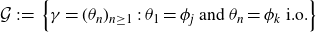 \begin{align*} \mathcal{G}\;:\!=\;\Big\{\gamma=(\theta_n)_{n\geq1}\,:\,\textrm{$\theta_1=\phi_j$ and $\theta_n=\phi_k$ i.o.} \Big\}\end{align*}
has positive $\bar{\nu}$
measure to prove Corollary 5·5. However, note that
$\bar{\nu}$
measure to prove Corollary 5·5. However, note that $\mathcal{G}=\mathcal{G}_1\cap\mathcal{G}_2$
where
$\mathcal{G}=\mathcal{G}_1\cap\mathcal{G}_2$
where
 \begin{align*} \mathcal{G}_1\;:\!=\;\Big\{\gamma=(\theta_n)_{n\geq1}\,:\,\textrm{$\theta_1=\phi_j$}\Big\}\;\;\;\;\textrm{and}\;\;\;\;\mathcal{G}_2\;:\!=\;\Big\{\gamma=(\theta_n)_{n\geq1}\,:\,\textrm{$\theta_n=\phi_k$ i.o.}\Big\}\end{align*}
respectively. On the other hand, $\bar{\nu}(\mathcal{G}_1)=\nu(\phi_j)>0$
since
$\bar{\nu}(\mathcal{G}_1)=\nu(\phi_j)>0$
since $\bar{\nu}$
is the product measure of a countable number of copies of
$\bar{\nu}$
is the product measure of a countable number of copies of $\nu$
on S; see [
Reference Jacod and ProtterJP03
, theorem 10·4]. Moreover, since
$\nu$
on S; see [
Reference Jacod and ProtterJP03
, theorem 10·4]. Moreover, since $\nu(\phi_k)>0$
, the Borel–Cantelli Theorem (specifically, the Monkey and Typewriter problem [
Reference GutGut13
, pp. 96-100]) implies that
$\nu(\phi_k)>0$
, the Borel–Cantelli Theorem (specifically, the Monkey and Typewriter problem [
Reference GutGut13
, pp. 96-100]) implies that $\bar{\nu}(\mathcal{G}_2)=1$
. Therefore,
$\bar{\nu}(\mathcal{G}_2)=1$
. Therefore,
 \begin{align*} \bar{\nu}(\mathcal{G})=\bar{\nu}(\mathcal{G}_1\cap\mathcal{G}_2)=\bar{\nu}(\mathcal{G}_1)=\nu(\phi_j)>0\end{align*}
as desired.
Finally, we are ready to prove Theorem 1·3 from the Introduction (which we restate for convenience below). Intuitively, this result shows that if $S=\{x^2+c_1,\dots, x^2+c_s\}$
for some polynomials
$S=\{x^2+c_1,\dots, x^2+c_s\}$
for some polynomials $c_i\in \mathbb{Z}[t]$
of fixed degree at most d, then as the cardinality of S grows, most such sets produce big arboreal representations over
$c_i\in \mathbb{Z}[t]$
of fixed degree at most d, then as the cardinality of S grows, most such sets produce big arboreal representations over $K=\mathbb{Q}(t)$
with positive probability; recall that big representations are those that are stable and also maximal infinitely often.
$K=\mathbb{Q}(t)$
with positive probability; recall that big representations are those that are stable and also maximal infinitely often.
Theorem 1·3. Let $d>0$
and
$d>0$
and $s\geq2$
, let
$s\geq2$
, let $\textrm{BigArb}(S)$
and
$\textrm{BigArb}(S)$
and $\mathcal{S}(d,s,B)$
be as in (1) and (2) above for
$\mathcal{S}(d,s,B)$
be as in (1) and (2) above for $K=\mathbb{Q}(t)$
, and let
$K=\mathbb{Q}(t)$
, and let
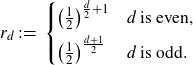
Then the following statements hold:
-
(1) if d is even, then
\begin{align*} \liminf_{B\rightarrow\infty}\frac{\#\Big\{S\in\mathcal{S}(d,s,B)\,:\,\bar{\nu}_S\big(\textrm{BigArb}(S,K)\big)>0\Big\}}{\#\mathcal{S}(d,s,B)}\geq 1-(1-r_d)^s;\end{align*}
-
(2) if d is odd, then
\begin{align*} \;\;\displaystyle{\liminf_{B\rightarrow\infty}}\frac{\#\Big\{S\in \mathcal{S}(d,s,B)\,:\,\bar{\nu}_S\big(\textrm{BigArb}(S,K)\big)>0\Big\}}{\#\mathcal{S}(d,s,B)} &\geq 1-(1-r_{d})^s-\Big(\frac{1}{2}\Big)^s \\[5pt] & + \Big(1-r_d-\frac{1}{2}\Big)^s. \end{align*}


In particular, when $d\geq1$
and
$d\geq1$
and $s\geq2$
are fixed, the number of sets
$s\geq2$
are fixed, the number of sets $S=\{x^2+c_1,\dots,x^2+c_s\}$
with
$S=\{x^2+c_1,\dots,x^2+c_s\}$
with $\deg(c_i)\leq d$
and which furnish with positive probability big arboreal representations approaches full density (in the set of all possible
$\deg(c_i)\leq d$
and which furnish with positive probability big arboreal representations approaches full density (in the set of all possible $S=\{x^2+c_1,\dots,x^2+c_s\}$
with
$S=\{x^2+c_1,\dots,x^2+c_s\}$
with $\deg(c_i)\leq d$
) as s grows.
$\deg(c_i)\leq d$
) as s grows.
Remark 10. In what follows, we let $x_B=(2B+1)$
to ease notation. Hence,
$x_B=(2B+1)$
to ease notation. Hence, $\#P_d(B)=x_B^{d+1}$
for all positive
$\#P_d(B)=x_B^{d+1}$
for all positive $B\in\mathbb{Z}$
since there are
$B\in\mathbb{Z}$
since there are $2B+1$
integers
$2B+1$
integers $\leq B$
and there are
$\leq B$
and there are $d+1$
possible terms in a polynomial of degree at most d. In particular,
$d+1$
possible terms in a polynomial of degree at most d. In particular, $\mathcal{S}(d,s,B)$
=
$\mathcal{S}(d,s,B)$
= $\binom{x_B^{d+1}}{s}$
by definition of
$\binom{x_B^{d+1}}{s}$
by definition of $\mathcal{S}(d,s,B)$
.
$\mathcal{S}(d,s,B)$
.
Remark 11. Recall that $\binom{X}{s}=\frac{X(X-1)\cdots(X-(s-1))}{s!}$
. Hence if we fix s and vary X, the binomial coefficient
$\binom{X}{s}=\frac{X(X-1)\cdots(X-(s-1))}{s!}$
. Hence if we fix s and vary X, the binomial coefficient $\binom{X}{s}$
is a polynomial of degree s in X with leading coefficient
$\binom{X}{s}$
is a polynomial of degree s in X with leading coefficient $(s!)^{-1}$
.
$(s!)^{-1}$
.
Proof. We proceed in cases depending on whether d is even or odd. The key distinction is that in the even case we may choose a single polynomial satisfying conditions (1) and (2) of Theorem 1·4. This is not possible in the odd case, unless $d=1$
.
$d=1$
.
Case (1): Assume that d is even. We begin by counting polynomials $c\in P_d(B)$
satisfying
$c\in P_d(B)$
satisfying $\frac{d}{dt}(\bar{c})=1$
in
$\frac{d}{dt}(\bar{c})=1$
in $\mathbb{F}_2[t]$
,
$\mathbb{F}_2[t]$
, $\deg(c)=d$
, and having odd leading term (which we call property (
*
)). This is clearly true of c if and only if:
$\deg(c)=d$
, and having odd leading term (which we call property (
*
)). This is clearly true of c if and only if:
 \begin{equation}c=\sum_{i=0}^d a_it^i,\;\,\textrm{$a_d$ is odd,}\; \textrm{$a_1$ is odd},\;\textrm{and}\;\textrm{$a_i$ is even for all odd indices $3\leq i\leq d-1$}.\end{equation}
In particular, after counting even or odd integers with absolute value at most B for each of the $d/2+1$
stipulated coefficients, we see that
$d/2+1$
stipulated coefficients, we see that
Here we use that $r_d= \big({1}/{2}\big)^{\frac{d}{2}+1}$
for even d. Hence, it follows from Remark 10 that there are
$r_d= \big({1}/{2}\big)^{\frac{d}{2}+1}$
for even d. Hence, it follows from Remark 10 that there are $(1-r_d)\cdot {x_B}^{d+1}+O({x_B}^{d})$
polynomials in
$(1-r_d)\cdot {x_B}^{d+1}+O({x_B}^{d})$
polynomials in $P_d(B)$
that do not satisfy property (
*
). In particular, there are
$P_d(B)$
that do not satisfy property (
*
). In particular, there are
 \begin{align*} \binom{(1-r_d)\cdot x_B^{d+1}+O({x_B}^{d})}{s}\end{align*}
sets in $\mathcal{S}(d,s,B)$
whose elements all fail to satisfy property (
*
). Therefore, there are
$\mathcal{S}(d,s,B)$
whose elements all fail to satisfy property (
*
). Therefore, there are
 \begin{equation}\binom{x_B^{d+1}}{s}-\binom{(1-r_d)\cdot x_B^{d+1}+O(x_B^{d})}{s}=\frac{(1-(1-r_d)^s)}{s!}x_B^{(d+1)s}+O(x_B^{(d+1)s-1})\end{equation}
sets in $\mathcal{S}(d,s,B)$
with at least one element satisfying property (
*
). Here we use also that the binomial coefficient
$\mathcal{S}(d,s,B)$
with at least one element satisfying property (
*
). Here we use also that the binomial coefficient $\binom{X}{s}$
is a polynomial of degree s in X with leading coefficient
$\binom{X}{s}$
is a polynomial of degree s in X with leading coefficient $(s!)^{-1}$
; see Remark 11.
$(s!)^{-1}$
; see Remark 11.
On the other hand, Corollary 5·5 implies that such sets $\{c_1,\dots,c_s\}\in \mathcal{S}(d,s,B)$
determine sets of quadratic polynomials
$\{c_1,\dots,c_s\}\in \mathcal{S}(d,s,B)$
determine sets of quadratic polynomials $S=\{x^2+c_1,\dots,x^2+c_s\}$
which furnish big arboreal representations over
$S=\{x^2+c_1,\dots,x^2+c_s\}$
which furnish big arboreal representations over $K=\mathbb{Q}(t)$
with positive probability. Hence, (13) and Corollary 5·5 together imply that
$K=\mathbb{Q}(t)$
with positive probability. Hence, (13) and Corollary 5·5 together imply that
 \begin{align*} \#\Big\{S\in\mathcal{S}(d,s,B)\,:\,\bar{\nu}_S\big(\textrm{BigArb}(S,K)\big)>0\Big\}\geq \frac{(1-(1-r_d)^s)}{s!}x_B^{(d+1)s}+O(x_B^{(d+1)s-1}).\end{align*}
In particular, after dividing the inequality above by
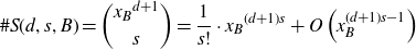 \begin{align*} \#S(d,s,B)=\binom{{x_B}^{d+1}}{s}=\frac{1}{s!}\cdot{x_B}^{(d+1)s}+O\left(x_B^{(d+1)s-1}\right) \end{align*}
and letting $B\rightarrow\infty$
, we see that
$B\rightarrow\infty$
, we see that
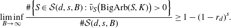 \begin{align*} \liminf_{B\rightarrow\infty}\frac{\#\Big\{S\in\mathcal{S}(d,s,B)\,:\,\bar{\nu}_S\big(\textrm{BigArb}(S,K)\big)>0\Big\}}{\#\mathcal{S}(d,s,B)}\geq 1-(1-r_d)^s. \end{align*}
Therefore, statement (1) of Theorem 1·3 holds for even d and fixed s as claimed.
Before we begin the proof of the case when d is odd, we need the following complementary form of the inclusion-exclusion principle.
Remark 12. Let $\mathcal{A}$
and
$\mathcal{A}$
and $\mathcal{B}$
be subsets of a finite set
$\mathcal{B}$
be subsets of a finite set $\mathcal{X}$
with complements
$\mathcal{X}$
with complements $\mathcal{A}^c$
and
$\mathcal{A}^c$
and $\mathcal{B}^c$
in
$\mathcal{B}^c$
in $\mathcal{X}$
respectively. Then
$\mathcal{X}$
respectively. Then $\#(\mathcal{A}\cap \mathcal{B})=\#\mathcal{X}-\#\mathcal{A}^c-\#\mathcal{B}^c+\#(\mathcal{A}^c\cap \mathcal{B}^c)$
; this follows directly from De Morgan’s Laws and the usual inclusion-exclusion principle.
$\#(\mathcal{A}\cap \mathcal{B})=\#\mathcal{X}-\#\mathcal{A}^c-\#\mathcal{B}^c+\#(\mathcal{A}^c\cap \mathcal{B}^c)$
; this follows directly from De Morgan’s Laws and the usual inclusion-exclusion principle.
Case (2): Assume that d is odd. We begin by counting polynomials $c\in P_d(B)$
satisfying
$c\in P_d(B)$
satisfying $\frac{d}{dt}(\bar{c})=1$
in
$\frac{d}{dt}(\bar{c})=1$
in $\mathbb{F}_2[t]$
and call this property (I). This is clearly true of c if and only if:
$\mathbb{F}_2[t]$
and call this property (I). This is clearly true of c if and only if:
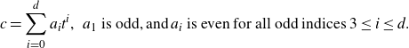 \begin{equation}c=\sum_{i=0}^d a_it^i,\;\, \textrm{$a_1$ is odd,}\;\textrm{and}\;\textrm{$a_i$ is even for all odd indices $3\leq i\leq d$}.\end{equation}
In particular, after counting even or odd integers with absolute value at most B for each of the $(d+1)/2$
stipulated coefficients, we see that
$(d+1)/2$
stipulated coefficients, we see that
Here we use that $r_d= \big({1}/{2}\big)^{\frac{d+1}{2}}$
for odd d. On the other hand, we say that
$r_d= \big({1}/{2}\big)^{\frac{d+1}{2}}$
for odd d. On the other hand, we say that $c\in P_d(B)$
has property (II) if it has degree d and odd leading term:
$c\in P_d(B)$
has property (II) if it has degree d and odd leading term:
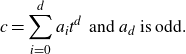 \begin{equation}c=\sum_{i=0}^d a_it^d\;\,\textrm{and $a_d$ is odd.} \end{equation}
Clearly properties (I) and (II) are disjoint events (i.e., there are no polynomials satisfying both properties) by examining the leading coefficient $a_d$
alone, and
$a_d$
alone, and
polynomials have property (II).
Now, with Corollary 5·5 and big arboreal representations in mind, we count sets in $\mathcal{S}(d,s,B)$
with at least one element satisfying property (I) and at least one element satisfying property (II). Do do this, let
$\mathcal{S}(d,s,B)$
with at least one element satisfying property (I) and at least one element satisfying property (II). Do do this, let $\mathcal{A}\subseteq \mathcal{S}(d,s,B)$
be the sets in
$\mathcal{A}\subseteq \mathcal{S}(d,s,B)$
be the sets in $\mathcal{S}(d,s,B)$
with at least one element satisfying property (I), and let
$\mathcal{S}(d,s,B)$
with at least one element satisfying property (I), and let $\mathcal{B}\subseteq \mathcal{S}(d,s,B)$
be the sets in
$\mathcal{B}\subseteq \mathcal{S}(d,s,B)$
be the sets in $\mathcal{S}(d,s,B)$
with at least one element satisfying property (II); that is, we want to count
$\mathcal{S}(d,s,B)$
with at least one element satisfying property (II); that is, we want to count $\#\mathcal{A}\cap \mathcal{B}$
. To do this, note first that (14) and Remark 10 imply that there are
$\#\mathcal{A}\cap \mathcal{B}$
. To do this, note first that (14) and Remark 10 imply that there are
 \begin{align*} \# P_d(B)-\Big(r_d\cdot x_B^{d+1}+O(x_B^{d})\Big)=(1-r_d)\cdot x_B^{d+1}+O(x_B^{d})\end{align*}
polynomials in $P_d(B)$
that do not have property (I). Therefore, there are
$P_d(B)$
that do not have property (I). Therefore, there are
 \begin{align*} \binom{(1-r_d)\cdot x_B^{d+1}+O(x_B^d)}{s}\end{align*}
sets in $\mathcal{S}(d,s,B)$
whose elements all fail to satisfy property (I). Equivalently,
$\mathcal{S}(d,s,B)$
whose elements all fail to satisfy property (I). Equivalently,
 \begin{equation}\#\mathcal{A}^c=\binom{(1-r_d)\cdot x_B^{d+1}+O(x_B^d)}{s};\end{equation}
here $\mathcal{A}^c$
denotes the complement of
$\mathcal{A}^c$
denotes the complement of $\mathcal{A}$
in
$\mathcal{A}$
in $\mathcal{S}(d,s,B)$
. Likewise, (15) and Remark 10 imply that there are
$\mathcal{S}(d,s,B)$
. Likewise, (15) and Remark 10 imply that there are
 \begin{align*} \# P_d(B)-\Big(\frac{1}{2}\cdot x_B^{d+1}+O(x_B^{d})\Big)=\frac{1}{2}\cdot x_B^{d+1}+O(x_B^{d})\end{align*}
polynomials in $P_d(B)$
that do not have property (II). Therefore, there are
$P_d(B)$
that do not have property (II). Therefore, there are
 \begin{align*} \binom{\frac{1}{2}\cdot x_B^{d+1}+O(x_B^d)}{s}\end{align*}
sets in $\mathcal{S}(d,s,B)$
whose elements all fail to satisfy property (II); Equivalently,
$\mathcal{S}(d,s,B)$
whose elements all fail to satisfy property (II); Equivalently,
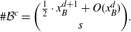 \begin{equation}\#\mathcal{B}^c=\binom{\frac{1}{2}\cdot x_B^{d+1}+O(x_B^d)}{s}.\end{equation}
Finally, before we can put all of the pieces above together, it remains to count $\#(\mathcal{A}^c\cap \mathcal{B}^c)$
. However,
$\#(\mathcal{A}^c\cap \mathcal{B}^c)$
. However, $\mathcal{A}^c\cap \mathcal{B}^c$
consists precisely of the sets in
$\mathcal{A}^c\cap \mathcal{B}^c$
consists precisely of the sets in $\mathcal{S}(d,s,B)$
whose elements all fail to satisfy (I) and all fail to satisfy (II). But, since (I) and (II) are disjoint events, there are exactly
$\mathcal{S}(d,s,B)$
whose elements all fail to satisfy (I) and all fail to satisfy (II). But, since (I) and (II) are disjoint events, there are exactly
 \begin{align*} \# P_d(B)-\Big(r_d\cdot x_B^{d+1}+O(x_B^{d})\Big)-\Big(\frac{1}{2}\cdot x_B^{d+1}+O(x_B^{d})\Big)=\big(1-r_d-\frac{1}{2}\big)\cdot x_B^{d+1}+O(x_B^{d})\end{align*}
polynomials that fail to satisfy (I) and fail to satisfy (II); here we use Remark 10, (14), and (15). Therefore, we see that
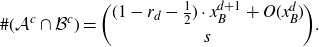 \begin{equation}\#(\mathcal{A}^c\cap \mathcal{B}^c)=\binom{(1-r_d-\frac{1}{2})\cdot x_B^{d+1}+O(x_B^d)}{s}.\end{equation}
In particular, (16), (17), (18), and the complementary form of the inclusion-exclusion principle in Remark 12 applied to $\mathcal{X}=\mathcal{S}(d,s,B)$
,
$\mathcal{X}=\mathcal{S}(d,s,B)$
, $\mathcal{A}$
and
$\mathcal{A}$
and $\mathcal{B}$
above imply that there are
$\mathcal{B}$
above imply that there are
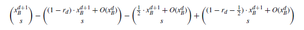 \begin{align*} {\binom{x_B^{d+1}}{s}-\binom{(1-r_d)\cdot x_B^{d+1}+O(x_B^d)}{s}-\binom{\frac{1}{2}\cdot x_B^{d+1}+O(x_B^d)}{s}+\binom{(1-r_d-\frac{1}{2})\cdot x_B^{d+1}+O(x_B^d)}{s}} \end{align*}
sets in $\mathcal{S}(d,s,B)$
with at least one element satisfying property (I) and at least one element satisfying property (II) (i.e., the expression above is
$\mathcal{S}(d,s,B)$
with at least one element satisfying property (I) and at least one element satisfying property (II) (i.e., the expression above is $\#\mathcal{A}\cap\mathcal{B}$
). Hence, there are
$\#\mathcal{A}\cap\mathcal{B}$
). Hence, there are
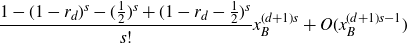 \begin{equation}\frac{1-(1-r_d)^s-(\frac{1}{2})^s+(1-r_d-\frac{1}{2})^s}{s!}x_B^{(d+1)s}+O(x_B^{(d+1)s-1})\end{equation}
sets in $\mathcal{S}(d,s,B)$
with at least one element satisfying property (I) and at least one element satisfying property (II); see also Remark 11. On the other hand, Corollary 5·5 implies that such sets
$\mathcal{S}(d,s,B)$
with at least one element satisfying property (I) and at least one element satisfying property (II); see also Remark 11. On the other hand, Corollary 5·5 implies that such sets $\{c_1,\dots,c_s\}\in\mathcal{S}(d,s,B)$
determine sets of quadratic polynomials
$\{c_1,\dots,c_s\}\in\mathcal{S}(d,s,B)$
determine sets of quadratic polynomials $S=\{x^2+c_1,\dots,x^2+c_s\}$
which furnish big arboreal representations over
$S=\{x^2+c_1,\dots,x^2+c_s\}$
which furnish big arboreal representations over $K=\mathbb{Q}(t)$
with positive probability. Hence, (19) and Corollary 5·5 together imply that
$K=\mathbb{Q}(t)$
with positive probability. Hence, (19) and Corollary 5·5 together imply that
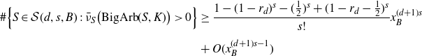 \begin{align*} \#\Big\{S\in\mathcal{S}(d,s,B)\,:\,\bar{\nu}_S\big(\textrm{BigArb}(S,K)\big)>0\Big\} & \geq \frac{1-(1-r_d)^s-(\frac{1}{2})^s+(1-r_d-\frac{1}{2})^s}{s!}x_B^{(d+1)s}\\[5pt] &+O(x_B^{(d+1)s-1}) \end{align*}
when d is odd. In particular, after dividing the inequality above by
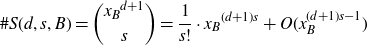 \begin{align*} \#S(d,s,B)=\binom{{x_B}^{d+1}}{s}=\frac{1}{s!}\cdot{x_B}^{(d+1)s}+O(x_B^{(d+1)s-1}) \end{align*}
and letting $B\rightarrow\infty$
, we see that
$B\rightarrow\infty$
, we see that
 \begin{align*} \displaystyle{\liminf_{B\rightarrow\infty}}\frac{\#\Big\{S\in \mathcal{S}(d,s,B)\,:\,\bar{\nu}_S\big(\textrm{BigArb}(S,K)\big)>0\Big\}}{\#\mathcal{S}(d,s,B)}\geq 1-(1-r_{d})^s-\Big(\frac{1}{2}\Big)^s+\Big(1-r_d-\frac{1}{2}\Big)^s\end{align*}
for odd d as claimed in part (2) of Theorem 1·3.
On the other hand, if we restrict ourselves to monic polynomials of fixed even degree, then we can we can improve Theorem 1·3 and count sets producing surjective arboreal representations with positive probability, instead of just big arboreal representations with positive probability. With this in mind, we fix a bit more notation: let $M_d(B)$
be the set of monic, degree-d polynomials in
$M_d(B)$
be the set of monic, degree-d polynomials in $\mathbb{Z}[t]$
whose coefficients all have absolute value at most B, and let
$\mathbb{Z}[t]$
whose coefficients all have absolute value at most B, and let
 \begin{align*} \mathcal{S}^{{Mon}}(d,s,B):\big\{\{c_1,c_2,\dots, c_s\}\,:\, c_i\in M_d(B)\big\}\end{align*}
be the set of s-element sets in $M_d(B)$
. Moreover, given an element
$M_d(B)$
. Moreover, given an element $\{c_1,\dots,c_s\}\in \mathcal{S}^{{Mon}}(d,s,B)$
we associate a set of quadratic polynomials with coefficients in
$\{c_1,\dots,c_s\}\in \mathcal{S}^{{Mon}}(d,s,B)$
we associate a set of quadratic polynomials with coefficients in $\mathbb{Z}[t]$
,
$\mathbb{Z}[t]$
,
 \begin{align*} S=S\big(\{c_1,\dots,c_s\}\big)=\{x^2+c_1,\dots, x^2+c_s\},\end{align*}
and study the sequences in S furnishing surjective arboreal representation over $K=\mathbb{Q}(t)$
:
$K=\mathbb{Q}(t)$
:
 \begin{align*} \textrm{SurArb}(S)\;:\!=\;\Big\{\gamma\in\Phi_S^{{sep}}\,:\, G_{\gamma,\,\mathbb{Q}(t)}=\operatorname{Aut}(T_\gamma)\Big\}.\end{align*}
In particular, we prove that most sets in $\mathcal{S}^{{Mon}}(d,s,B)$
produce surjective representations with positive probability as s grows.
$\mathcal{S}^{{Mon}}(d,s,B)$
produce surjective representations with positive probability as s grows.
Theorem 5·6. Let $d>0$
, let
$d>0$
, let $s\geq2$
, and let
$s\geq2$
, and let $\mathcal{S}^{{Mon}}(d,s,B)$
and
$\mathcal{S}^{{Mon}}(d,s,B)$
and $\textrm{SurArb}(S)$
be as above. If d is even, then
$\textrm{SurArb}(S)$
be as above. If d is even, then
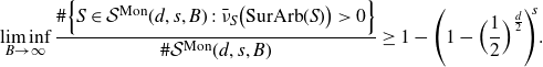 \begin{align*} \liminf_{B\rightarrow\infty}\frac{\#\Big\{S\in \mathcal{S}^{{Mon}}(d,s,B)\,:\,\bar{\nu}_S\big(\textrm{SurArb}(S)\big)>0\Big\}}{\#\mathcal{S}^{{Mon}}(d,s,B)}\geq 1-\Bigg(1-\Big(\frac{1}{2}\Big)^{\frac{d}{2}}\Bigg)^{\hspace{-.1cm}s}.\end{align*}
In particular, when $d\geq2$
is fixed and even, almost all sets
$d\geq2$
is fixed and even, almost all sets $S=\{x^2+c_1,\dots,x^2+c_s\}$
with
$S=\{x^2+c_1,\dots,x^2+c_s\}$
with $c_i\in M_d$
furnish surjective arboreal representations with positive probability as
$c_i\in M_d$
furnish surjective arboreal representations with positive probability as $s\rightarrow\infty$
.
$s\rightarrow\infty$
.
Proof. The proof is very similar to that of statement (1) of Theorem 1·3 (only now the leading terms are fixed). In particular, it is straightforward to check that $\#M_d(B)=x_B^d$
and
$\#M_d(B)=x_B^d$
and
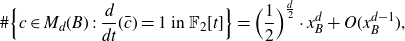 \begin{equation}\#\Big\{c\in M_d(B)\,:\,\textrm{$\frac{d}{dt}(\bar{c})=1$ in $\mathbb{F}_2[t]$}\Big\}=\Big(\frac{1}{2}\Big)^{\frac{d}{2}}\cdot x_B^d +O(x_B^{d-1}),\end{equation}
since the c’s above must have even coefficients at every odd-powered term, except for the linear term, which must be odd - that is, there is a parity stipulation on the coefficients of c at every odd-powered term (and $d/2$
such terms). Therefore, similar to Case (1) in the proof of Theorem 1·3, there are
$d/2$
such terms). Therefore, similar to Case (1) in the proof of Theorem 1·3, there are
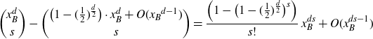 \begin{equation}\binom{x_B^d}{s}-\binom{\big(1-({\frac{1}{2}})^{\frac{d}{2}}\big)\cdot x_B^{d}+O({x_B}^{d-1})}{s}=\frac{\Big(1-\big(1-({\frac{1}{2}})^{\frac{d}{2}}\big)^s\Big)}{s!}\,x_B^{ds}+O(x_B^{ds-1})\end{equation}
sets in $\mathcal{S}^{\textrm{Mon}}(d,s,B)$
with at least one term
$\mathcal{S}^{\textrm{Mon}}(d,s,B)$
with at least one term $c_j\in\mathbb{Z}[t]$
satisfying
$c_j\in\mathbb{Z}[t]$
satisfying $\frac{d}{dt}(\bar{c}_j)=1$
in
$\frac{d}{dt}(\bar{c}_j)=1$
in $\mathbb{F}_2[t]$
. On the other hand, such collections determine sets of quadratic polynomials
$\mathbb{F}_2[t]$
. On the other hand, such collections determine sets of quadratic polynomials $S=\{x^2+c_1,\dots,x^2+c_s\}$
which furnish surjective arboreal representations over
$S=\{x^2+c_1,\dots,x^2+c_s\}$
which furnish surjective arboreal representations over $\mathbb{Q}(t)$
with positive probability by Theorem 1·4: the sequences
$\mathbb{Q}(t)$
with positive probability by Theorem 1·4: the sequences $\gamma=(\theta_n)_{n\geq1}$
with
$\gamma=(\theta_n)_{n\geq1}$
with $\theta_1=x^2+c_j$
produce maximal extensions for every n since condition (2) of Theorem 1·4 is satisfied by all
$\theta_1=x^2+c_j$
produce maximal extensions for every n since condition (2) of Theorem 1·4 is satisfied by all $c\in M_d(B)$
. Therefore, it follows from (21) that
$c\in M_d(B)$
. Therefore, it follows from (21) that
 \begin{equation}\#\Big\{S\in\mathcal{S}^{\textrm{Mon}}(d,s,B) \,:\,\bar{\nu}_S\big(\textrm{SurArb}(S)\big)>0\Big\}\geq \frac{\Big(1-\big(1-({\frac{1}{2}})^{\frac{d}{2}}\big)^s\Big)}{s!}\,x_B^{ds}+O(x_B^{ds-1}).\end{equation}
In particular, after dividing both sides of (22) by
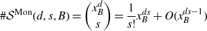 \begin{align*} \#\mathcal{S}^{\textrm{Mon}}(d,s,B)=\binom{x_B^d}{s}=\frac{1}{s!}x_B^{ds}+O(x_B^{ds-1})\end{align*}
and letting $B\rightarrow\infty$
, we obtain the lower bound
$B\rightarrow\infty$
, we obtain the lower bound
 \begin{align*} \liminf_{B\rightarrow\infty}\frac{\#\Big\{S\in \mathcal{S}^{{Mon}}(d,s,B)\,:\,\bar{\nu}_S\big(\textrm{SurArb}(S)\big)>0\Big\}}{\#\mathcal{S}^{{Mon}}(d,s,B)}\geq 1-\Bigg(1-\Big(\frac{1}{2}\Big)^{\frac{d}{2}}\Bigg)^{\hspace{-.1cm}s}\end{align*}
in Theorem 5·6 as claimed.
6. Applications to density of prime divisors
Let K be a number field with ring of integers $\mathcal{O}_K$
and let
$\mathcal{O}_K$
and let $\gamma=(\theta_n)_{n\geq1}$
for some
$\gamma=(\theta_n)_{n\geq1}$
for some $\theta_n\in K[x]$
. In this section we consider sequences of the form
$\theta_n\in K[x]$
. In this section we consider sequences of the form $(\gamma_n(a_0))_{n \geq 0}$
, where
$(\gamma_n(a_0))_{n \geq 0}$
, where $a_0 \in K$
,
$a_0 \in K$
, $\gamma_0(x) = x$
, and
$\gamma_0(x) = x$
, and $\gamma_n(x) = (\theta_1 \circ \cdots \circ \theta_n)(x)$
for
$\gamma_n(x) = (\theta_1 \circ \cdots \circ \theta_n)(x)$
for $n \geq 1$
. In particular, we are interested in the set of prime ideal divisors of our sequence, namely
$n \geq 1$
. In particular, we are interested in the set of prime ideal divisors of our sequence, namely
 \begin{align*}P(\gamma, a_0) \;:\!=\; \{{\mathfrak{p}} \subset {\mathcal O}_K \;:\; \textrm{${\mathfrak{p}}$ is prime and ${\mathfrak{p}} \mid \gamma_n(a_0)$ for at least one $n \geq 0$ with $\gamma_n(a_0) \neq 0$}\}.\end{align*}
Recall that the natural density of a set T of primes in ${\mathcal O}_K$
is
${\mathcal O}_K$
is
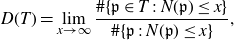 \begin{equation*}D(T) = \lim_{x \to \infty} \frac{\#\{{\mathfrak{p}} \in T \;:\; N({\mathfrak{p}}) \leq x\}}{\#\{{\mathfrak{p}} \;:\; N({\mathfrak{p}}) \leq x\}},\end{equation*}
provided that this limit exists. Here $N({\mathfrak{p}})$
denotes the norm of
$N({\mathfrak{p}})$
denotes the norm of ${\mathfrak{p}}$
. Likewise, we define the upper density
${\mathfrak{p}}$
. Likewise, we define the upper density $D^+(T)$
by replacing the limit above with a
$D^+(T)$
by replacing the limit above with a $\limsup$
. In particular, our goal is to determine
$\limsup$
. In particular, our goal is to determine $D(P(\gamma, a_0))$
in certain cases.
$D(P(\gamma, a_0))$
in certain cases.
As a first step, we relate $D(P(\gamma, a_0))$
to the Galois group
$D(P(\gamma, a_0))$
to the Galois group $G_{\gamma, n, K}$
of
$G_{\gamma, n, K}$
of $K_n(\gamma)/K$
. Throughout this section, we suppress the dependence on
$K_n(\gamma)/K$
. Throughout this section, we suppress the dependence on $\gamma$
and K and write
$\gamma$
and K and write $G_n$
in place of
$G_n$
in place of $G_{\gamma, n, K}$
. The group
$G_{\gamma, n, K}$
. The group $G_n$
acts naturally on the roots
$G_n$
acts naturally on the roots $R_n$
of
$R_n$
of $\gamma_n$
(note that
$\gamma_n$
(note that $R_n$
is the nth level of the tree
$R_n$
is the nth level of the tree $T_{\gamma,n},$
which we denote just by
$T_{\gamma,n},$
which we denote just by $T_n$
). Define the fixed-point proportion of
$T_n$
). Define the fixed-point proportion of $G_n$
to be
$G_n$
to be
Note that since $G_n$
acts on
$G_n$
acts on $T_n$
by tree automorphisms for every n, we have that the sequence
$T_n$
by tree automorphisms for every n, we have that the sequence $(\textrm{FPP}(G_n))_{n \geq 1}$
is non-increasing, and hence its limit must exist.
$(\textrm{FPP}(G_n))_{n \geq 1}$
is non-increasing, and hence its limit must exist.
The following theorem is a version of [ Reference JonesJon08 , theorem 2·1], adapted to the present circumstances.
Theorem 6·1. Assume that $\gamma_n$
is separable over K for all
$\gamma_n$
is separable over K for all $n \geq 1$
, and let
$n \geq 1$
, and let $a_0 \in K$
. Then
$a_0 \in K$
. Then
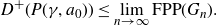 \begin{equation} D^+(P(\gamma, a_0)) \leq \lim_{n \to \infty} {FPP}(G_n).\end{equation}
Remark 13. Our applications of Theorem 6·1 are all in the case where ${FPP}(G_n) \to 0$
, in which case (24) implies that
${FPP}(G_n) \to 0$
, in which case (24) implies that $D(P(\gamma, a_0))$
exists (and equals 0). In general when
$D(P(\gamma, a_0))$
exists (and equals 0). In general when $\lim_{n \to \infty} {FPP}(G_n) > 0$
we do not a priori know that
$\lim_{n \to \infty} {FPP}(G_n) > 0$
we do not a priori know that $D(P(\gamma, a_0))$
exists. In the setting of iteration of a single rational map
$D(P(\gamma, a_0))$
exists. In the setting of iteration of a single rational map $\phi$
, there are known cases where
$\phi$
, there are known cases where $\lim_{n \to \infty} {FPP}(G_n) > 0$
, and they occur when
$\lim_{n \to \infty} {FPP}(G_n) > 0$
, and they occur when $\phi$
is a finite quotient of an affine map of an abelian algebraic group. In this situation the extra structure often allows one to show directly that the relevant density of prime divisors exists (and equals
$\phi$
is a finite quotient of an affine map of an abelian algebraic group. In this situation the extra structure often allows one to show directly that the relevant density of prime divisors exists (and equals $\lim_{n \to \infty} {FPP}(G_n)$
). See e.g. [
Reference Jones and RouseJR10
, theorem 3·2].
$\lim_{n \to \infty} {FPP}(G_n)$
). See e.g. [
Reference Jones and RouseJR10
, theorem 3·2].
Proof. Denote the discriminant of $\gamma_n$
by
$\gamma_n$
by $\textrm{Disc}(\gamma_n)$
, and for a prime
$\textrm{Disc}(\gamma_n)$
, and for a prime ${\mathfrak{p}}$
of
${\mathfrak{p}}$
of ${\mathcal O}_K$
let
${\mathcal O}_K$
let $v_{\mathfrak{p}}$
be the
$v_{\mathfrak{p}}$
be the ${\mathfrak{p}}$
-adic valuation. Let
${\mathfrak{p}}$
-adic valuation. Let $B_n$
be the following finite set of primes of
$B_n$
be the following finite set of primes of ${\mathcal O}_K$
:
${\mathcal O}_K$
:
and note that if ${\mathfrak{p}} \not\in B_n$
then
${\mathfrak{p}} \not\in B_n$
then $\gamma_n$
has good reduction, i.e. reducing
$\gamma_n$
has good reduction, i.e. reducing $\gamma_n$
coefficient-wise modulo
$\gamma_n$
coefficient-wise modulo ${\mathfrak{p}}$
yields a polynomial
${\mathfrak{p}}$
yields a polynomial $\widetilde{\gamma_n}$
in
$\widetilde{\gamma_n}$
in ${\mathcal O}_K/{\mathfrak{p}}$
of degree
${\mathcal O}_K/{\mathfrak{p}}$
of degree $\deg(\gamma_n)$
. In particular, every root
$\deg(\gamma_n)$
. In particular, every root $\alpha$
of
$\alpha$
of $\gamma_n$
satisfies
$\gamma_n$
satisfies $v_{\mathfrak{p}}(\alpha) \geq 0$
. Fix
$v_{\mathfrak{p}}(\alpha) \geq 0$
. Fix $n \geq 1$
, and let
$n \geq 1$
, and let
Assume that ${\mathfrak{p}} \in \Omega_n$
and take
${\mathfrak{p}} \in \Omega_n$
and take $N > n$
. If
$N > n$
. If $\gamma_N(x) \equiv 0 \bmod{{\mathfrak{p}}}$
has a solution in K, then because
$\gamma_N(x) \equiv 0 \bmod{{\mathfrak{p}}}$
has a solution in K, then because $\gamma_N = \gamma_n \circ \theta_{n+1} \circ \cdots \circ \theta_N$
, it follows that
$\gamma_N = \gamma_n \circ \theta_{n+1} \circ \cdots \circ \theta_N$
, it follows that $\gamma_n(x) \equiv 0 \bmod{{\mathfrak{p}}}$
has a solution in K, and thus
$\gamma_n(x) \equiv 0 \bmod{{\mathfrak{p}}}$
has a solution in K, and thus $\Omega_n \subseteq R_n$
. Observe that there are only finitely many prime
$\Omega_n \subseteq R_n$
. Observe that there are only finitely many prime ${\mathfrak{p}}$
with
${\mathfrak{p}}$
with ${\mathfrak{p}} \mid \gamma_N(a_0)$
and
${\mathfrak{p}} \mid \gamma_N(a_0)$
and $\gamma_N(a_0) \neq 0$
for some
$\gamma_N(a_0) \neq 0$
for some $N < n$
, and this together with the finiteness of
$N < n$
, and this together with the finiteness of $B_n$
imply that
$B_n$
imply that $R_n$
and the complement
$R_n$
and the complement $P(\gamma, a_0)^c$
differ by a finite set of primes, which we denote by
$P(\gamma, a_0)^c$
differ by a finite set of primes, which we denote by $F_n$
.
$F_n$
.
Assume for a moment that $D(\Omega_n)$
exists and equals
$D(\Omega_n)$
exists and equals $d_n$
. Let
$d_n$
. Let $\epsilon > 0$
and take
$\epsilon > 0$
and take $x_0$
large enough so that if
$x_0$
large enough so that if $x \geq x_0$
then both
$x \geq x_0$
then both
 \begin{equation} \frac{\#\{{\mathfrak{p}} \in \Omega_n \;:\; N({\mathfrak{p}}) \leq x\}}{\#\{{\mathfrak{p}} \;:\; N({\mathfrak{p}}) \leq x\}} > d_n - \epsilon/2 \quad \textrm{and} \quad \frac{\#\{{\mathfrak{p}} \in F_n \;:\; N({\mathfrak{p}}) \leq x\}}{\#\{{\mathfrak{p}} \;:\; N({\mathfrak{p}}) \leq x\}} < \epsilon/2.\end{equation}
The first inequality in (25) implies that ${\#\{{\mathfrak{p}} \in R_n \;:\; N({\mathfrak{p}}) \leq x\}}/{\#\{{\mathfrak{p}} \;:\; N({\mathfrak{p}}) \leq x\}} > d_n - \epsilon/2$
, and together with the second inequality in (25) this gives
${\#\{{\mathfrak{p}} \in R_n \;:\; N({\mathfrak{p}}) \leq x\}}/{\#\{{\mathfrak{p}} \;:\; N({\mathfrak{p}}) \leq x\}} > d_n - \epsilon/2$
, and together with the second inequality in (25) this gives
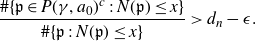 \begin{align*}\frac{\#\{{\mathfrak{p}} \in P(\gamma, a_0)^c \;:\; N({\mathfrak{p}}) \leq x\}}{\#\{{\mathfrak{p}} \;:\; N({\mathfrak{p}}) \leq x\}} > d_n - \epsilon.\end{align*}
This implies that ${\#\{{\mathfrak{p}} \in P(\gamma, a_0) \;:\; N({\mathfrak{p}}) \leq x\}}/{\#\{{\mathfrak{p}} \;:\; N({\mathfrak{p}}) \leq x\}} < (1 - d_n) + \epsilon,$
from which we obtain
${\#\{{\mathfrak{p}} \in P(\gamma, a_0) \;:\; N({\mathfrak{p}}) \leq x\}}/{\#\{{\mathfrak{p}} \;:\; N({\mathfrak{p}}) \leq x\}} < (1 - d_n) + \epsilon,$
from which we obtain $D^+(P(\gamma, a_0)) < 1-d_n$
, and thus
$D^+(P(\gamma, a_0)) < 1-d_n$
, and thus $D^+(P(\gamma, a_0)) \leq \lim_{n \to \infty} (1-d_n)$
.
$D^+(P(\gamma, a_0)) \leq \lim_{n \to \infty} (1-d_n)$
.
The proof will be complete once we show that $D(\Omega_n)$
exists and equals
$D(\Omega_n)$
exists and equals $1 - \textrm{FPP}(G_n)$
. If
$1 - \textrm{FPP}(G_n)$
. If ${\mathfrak{p}} \nmid \textrm{Disc}(\gamma_n)$
, then
${\mathfrak{p}} \nmid \textrm{Disc}(\gamma_n)$
, then ${\mathfrak{p}}$
cannot divide the field discriminant of
${\mathfrak{p}}$
cannot divide the field discriminant of $K_n(\gamma)/K$
; see, for instance, [
Reference NarkiewiczNar04
, corollary 2, p. 157]. Hence, such
$K_n(\gamma)/K$
; see, for instance, [
Reference NarkiewiczNar04
, corollary 2, p. 157]. Hence, such ${\mathfrak{p}}$
are unramified in the extension
${\mathfrak{p}}$
are unramified in the extension $K_n(\gamma)/K$
. Now
$K_n(\gamma)/K$
. Now $\gamma_n(x) \equiv 0 \pmod{{\mathfrak{p}}}$
having a solution in K is equivalent to
$\gamma_n(x) \equiv 0 \pmod{{\mathfrak{p}}}$
having a solution in K is equivalent to $\widetilde{\gamma_n}$
having at least one linear factor in
$\widetilde{\gamma_n}$
having at least one linear factor in $({\mathcal O}_K/{\mathfrak{p}})[x]$
. Except for possibly finitely many
$({\mathcal O}_K/{\mathfrak{p}})[x]$
. Except for possibly finitely many ${\mathfrak{p}}$
, this implies that
${\mathfrak{p}}$
, this implies that ${\mathfrak{p}}{\mathcal O}_L = \mathfrak{P}_1 \cdots \mathfrak{P}_r$
, where
${\mathfrak{p}}{\mathcal O}_L = \mathfrak{P}_1 \cdots \mathfrak{P}_r$
, where $L/K$
is obtained by adjoining a root of
$L/K$
is obtained by adjoining a root of $\gamma_n$
,
$\gamma_n$
, ${\mathcal O}_L$
is the ring of integers of L, and at least one of the
${\mathcal O}_L$
is the ring of integers of L, and at least one of the $\mathfrak{P}_i$
has residue class degree one [
Reference NarkiewiczNar04
, theorem 4·12]. This is equivalent to the disjoint cycle decomposition of the Frobenius conjugacy class at
$\mathfrak{P}_i$
has residue class degree one [
Reference NarkiewiczNar04
, theorem 4·12]. This is equivalent to the disjoint cycle decomposition of the Frobenius conjugacy class at ${\mathfrak{p}}$
having a fixed point (in the natural permutation representation of
${\mathfrak{p}}$
having a fixed point (in the natural permutation representation of $G_n$
on the roots
$G_n$
on the roots $R_n$
of
$R_n$
of $\gamma_n$
). From the Chebotarev Density Theorem it follows [
Reference NarkiewiczNar04
, proposition 7·15] that the density of
$\gamma_n$
). From the Chebotarev Density Theorem it follows [
Reference NarkiewiczNar04
, proposition 7·15] that the density of ${\mathfrak{p}}$
with
${\mathfrak{p}}$
with ${\mathfrak{p}}{\mathcal O}_L$
having such a decomposition exists and equals
${\mathfrak{p}}{\mathcal O}_L$
having such a decomposition exists and equals $\textrm{FPP}(G_n)$
. We have thus shown that
$\textrm{FPP}(G_n)$
. We have thus shown that $D(\Omega_n^c)$
exists and equals
$D(\Omega_n^c)$
exists and equals $\textrm{FPP}(G_n)$
, and the proof is complete.
$\textrm{FPP}(G_n)$
, and the proof is complete.
We now tackle the problem of computing $\lim_{n \to \infty} \textrm{FPP}(G_n)$
for certain choices of
$\lim_{n \to \infty} \textrm{FPP}(G_n)$
for certain choices of $\gamma_n$
. A convenient vehicle for this is a stochastic process that encodes fixed-point information about the action of elements of
$\gamma_n$
. A convenient vehicle for this is a stochastic process that encodes fixed-point information about the action of elements of $G_\infty \;:\!=\; \varprojlim G_n$
on
$G_\infty \;:\!=\; \varprojlim G_n$
on $R_n$
for each n. Let
$R_n$
for each n. Let $\textbf{P}$
be the Harr measure on
$\textbf{P}$
be the Harr measure on $G_\infty$
, normalized so that
$G_\infty$
, normalized so that $\textbf{P}(G_\infty) = 1$
. Each
$\textbf{P}(G_\infty) = 1$
. Each $g \in G_\infty$
acts on
$g \in G_\infty$
acts on $R_n$
for all
$R_n$
for all $n \geq 1$
. We define random variables
$n \geq 1$
. We define random variables $X_1, X_2, \ldots$
by
$X_1, X_2, \ldots$
by
We call the stochastic process $(X_1, X_2, \ldots)$
the fixed-point process of
$(X_1, X_2, \ldots)$
the fixed-point process of $G_\infty$
. In particular, note that
$G_\infty$
. In particular, note that $\textrm{FPP}(G_n) = \textbf{P}(X_n > 0)$
.
$\textrm{FPP}(G_n) = \textbf{P}(X_n > 0)$
.
Definition 6·2. A stochastic process $(X_0, X_1, X_2, \ldots)$
taking values in
$(X_0, X_1, X_2, \ldots)$
taking values in $\mathbb{Z}$
is a martingale if for all
$\mathbb{Z}$
is a martingale if for all $n \geq 1$
and any
$n \geq 1$
and any $t_i \in \mathbb{Z}$
,
$t_i \in \mathbb{Z}$
,
 \begin{align*} E(X_n \mid X_{0} = t_{0}, X_1 = t_1, \ldots, X_{n-1} = t_{n-1}) = t_{n-1}.\end{align*}
We call $(X_0, X_1, X_2, \ldots)$
an eventual martingale if for some
$(X_0, X_1, X_2, \ldots)$
an eventual martingale if for some $n_0 \geq 1$
the tail end process
$n_0 \geq 1$
the tail end process $X_{n_0}, X_{n_0 + 1}, X_{n_0 + 2}, \ldots $
is a martingale.
$X_{n_0}, X_{n_0 + 1}, X_{n_0 + 2}, \ldots $
is a martingale.
A standard martingale convergence theorem shows the following agreeable property of eventual martingales, which is corollary 2·3 of [ Reference JonesJon08 ]:
Proposition 6·3. Suppose that the Galois process of $G_\infty$
is an eventual martingale. Then
$G_\infty$
is an eventual martingale. Then
 \begin{align*} \textbf{P}(\{g \in G_\infty \;:\; \textrm{$X_1(g), X_2(g), \ldots$ is eventually constant}\}) = 1.\end{align*}
Denote the Galois group of $K_n(\gamma)/K_{n-1}(\gamma)$
by
$K_n(\gamma)/K_{n-1}(\gamma)$
by $H_n$
. Proposition 6·3 allows us to obtain significant information about the Galois process of
$H_n$
. Proposition 6·3 allows us to obtain significant information about the Galois process of $G_\infty$
from knowledge of only an infinite number of
$G_\infty$
from knowledge of only an infinite number of $H_n$
. The following is lemma 5·3 of [
Reference JonesJon07
]:
$H_n$
. The following is lemma 5·3 of [
Reference JonesJon07
]:
Lemma 6·4 ([
Reference JonesJon07
]). Assume that all $\theta_i$
are quadratic, and let
$\theta_i$
are quadratic, and let $n \geq 2$
. If
$n \geq 2$
. If $H_n$
is maximal, then for any m with
$H_n$
is maximal, then for any m with $1 \leq m < n$
and any integer
$1 \leq m < n$
and any integer $u > 0$
,
$u > 0$
,
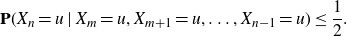 \begin{equation} \textbf{P}(X_n = u \mid X_m = u, X_{m+1} = u, \ldots, X_{n-1} = u) \leq \frac{1}{2}.\end{equation}
Indeed, if u is not of the form 2w for $1 \leq w \leq 2^{m-1}$
, then
$1 \leq w \leq 2^{m-1}$
, then $\textbf{P}(X_n = u) = 0$
. Otherwise, lemma 5·2 of [
Reference JonesJon07
] shows that the maximality of
$\textbf{P}(X_n = u) = 0$
. Otherwise, lemma 5·2 of [
Reference JonesJon07
] shows that the maximality of $H_n$
forces
$H_n$
forces $(X_n \, | \, (X_{n-1} = u))$
to have the same distribution as flipping u fair coins, with heads counting 2 and tails 0. Thus the left-hand side of (26) is
$(X_n \, | \, (X_{n-1} = u))$
to have the same distribution as flipping u fair coins, with heads counting 2 and tails 0. Thus the left-hand side of (26) is $\left(\substack{u\\ u/2}\right) \frac{1}{2^u}$
, which is easily seen to be at most
$\left(\substack{u\\ u/2}\right) \frac{1}{2^u}$
, which is easily seen to be at most $1/2$
.
$1/2$
.
To make use of Proposition 6·3 and Lemma 6·4, we wish to give conditions on $\gamma$
under which the fixed point process of
$\gamma$
under which the fixed point process of $G_\infty$
is an eventual martingale. We make the assumption that all
$G_\infty$
is an eventual martingale. We make the assumption that all $\theta_i$
are quadratic, and use arguments similar to those in [
Reference JonesJon08
, section 2].
$\theta_i$
are quadratic, and use arguments similar to those in [
Reference JonesJon08
, section 2].
Theorem 6·5. Suppose that for all $n \geq 1$
,
$n \geq 1$
, $\theta_n$
is quadratic and
$\theta_n$
is quadratic and $\gamma_n$
is irreducible over K. If
$\gamma_n$
is irreducible over K. If $H_n$
is non-trivial for all n sufficiently large, then the fixed point process of
$H_n$
is non-trivial for all n sufficiently large, then the fixed point process of $G_\infty$
is an eventual martingale.
$G_\infty$
is an eventual martingale.
Proof. First note that since K is a number field, the irreducibility of $\gamma_n$
over K implies that
$\gamma_n$
over K implies that $\gamma_n$
is separable over K. From Lemma 2·4 and theorem 2·5 of [
Reference JonesJon08
] it follows that the present theorem is proved provided that the following holds: there exists
$\gamma_n$
is separable over K. From Lemma 2·4 and theorem 2·5 of [
Reference JonesJon08
] it follows that the present theorem is proved provided that the following holds: there exists $n_0 \geq 1$
such that for all
$n_0 \geq 1$
such that for all $n \geq n_0$
and every root
$n \geq n_0$
and every root $\alpha$
of
$\alpha$
of $\gamma_{n-1}$
, the polynomial
$\gamma_{n-1}$
, the polynomial $\theta_n - \alpha$
is irreducible over
$\theta_n - \alpha$
is irreducible over $K_{n-1}(\gamma)$
. Let
$K_{n-1}(\gamma)$
. Let $n_0$
be such that
$n_0$
be such that $H_n$
is non-trivial for
$H_n$
is non-trivial for $n \geq n_0$
, and fix
$n \geq n_0$
, and fix $n \geq n_0$
. Observe that
$n \geq n_0$
. Observe that
 \begin{equation} \gamma_n = \prod_{\alpha \in \gamma_{n-1}^{-1}(0)} (\theta_n(x) - \alpha).\end{equation}
Because $H_n$
is non-trivial, there must be some
$H_n$
is non-trivial, there must be some $\alpha$
such that
$\alpha$
such that $\theta_n - \alpha$
has a root not in
$\theta_n - \alpha$
has a root not in $K_{n-1}(\gamma)$
. Because
$K_{n-1}(\gamma)$
. Because $\theta_n$
has degree 2, this implies that
$\theta_n$
has degree 2, this implies that $\theta_n - \alpha$
is irreducible over
$\theta_n - \alpha$
is irreducible over $K_{n-1}(\gamma)$
. By hypothesis,
$K_{n-1}(\gamma)$
. By hypothesis, $\gamma_{n-1}$
is irreducible over K, and hence
$\gamma_{n-1}$
is irreducible over K, and hence $G_{n-1}$
acts transitively on the roots of
$G_{n-1}$
acts transitively on the roots of $\gamma_{n-1}$
. It follows that
$\gamma_{n-1}$
. It follows that $\theta_n - \alpha$
is irreducible over
$\theta_n - \alpha$
is irreducible over $K_{n-1}(\gamma)$
for all
$K_{n-1}(\gamma)$
for all $\alpha$
, as desired.
$\alpha$
, as desired.
We are now in a position to prove the main result of this section, which we restate from the Introduction
Theorem 1·5. Let K be a number field and let $S = \{x^2 + c_1, \ldots, x^2 + c_s\}$
with
$S = \{x^2 + c_1, \ldots, x^2 + c_s\}$
with $c_i \in K$
. Suppose that
$c_i \in K$
. Suppose that $\gamma \in {BigArb}(S,K)$
. Then
$\gamma \in {BigArb}(S,K)$
. Then $D(P(\gamma, a_0)) = 0$
for any
$D(P(\gamma, a_0)) = 0$
for any $a_0 \in K$
.
$a_0 \in K$
.
Proof. As in the discussion above, write $G_\infty$
for
$G_\infty$
for $G_{\gamma, K}$
, the inverse limit of the
$G_{\gamma, K}$
, the inverse limit of the $G_n$
, and write
$G_n$
, and write $H_n$
for the Galois group of
$H_n$
for the Galois group of $K_n(\gamma)/K_{n-1}(\gamma)$
. We first claim that
$K_n(\gamma)/K_{n-1}(\gamma)$
. We first claim that $H_n$
is non-trivial for all sufficiently large n, which by Theorem 6·5 shows that the fixed point process of
$H_n$
is non-trivial for all sufficiently large n, which by Theorem 6·5 shows that the fixed point process of $G_\infty$
is an eventual martingale.
$G_\infty$
is an eventual martingale.
Let ${\mathfrak{C}}$
be the partition of
${\mathfrak{C}}$
be the partition of $T_n$
into the sets
$T_n$
into the sets $\{\textrm{roots of $_n(x)$ -}\},$
where
$\{\textrm{roots of $_n(x)$ -}\},$
where $\alpha$
varies over roots of
$\alpha$
varies over roots of $\theta_n$
, as in (27). Let
$\theta_n$
, as in (27). Let $\sigma_{{\mathfrak{C}}} \in {\rm Sym} (V_n)$
be the permutation associated to
$\sigma_{{\mathfrak{C}}} \in {\rm Sym} (V_n)$
be the permutation associated to ${\mathfrak{C}}$
, i.e. the unique permutation whose orbits are precisely the sets belonging to
${\mathfrak{C}}$
, i.e. the unique permutation whose orbits are precisely the sets belonging to ${\mathfrak{C}}$
. We wish to show that
${\mathfrak{C}}$
. We wish to show that $\sigma_{{\mathfrak{C}}} \in G_n$
for n sufficiently large, and then the fact that
$\sigma_{{\mathfrak{C}}} \in G_n$
for n sufficiently large, and then the fact that $\sigma_{\mathfrak{C}}$
only acts non-trivially on fibers of
$\sigma_{\mathfrak{C}}$
only acts non-trivially on fibers of $\theta_n$
implies that
$\theta_n$
implies that $\sigma_{\mathfrak{C}} \in H_n$
, whence
$\sigma_{\mathfrak{C}} \in H_n$
, whence $H_n$
is non-trivial.
$H_n$
is non-trivial.
Because S contains only quadratic polynomials, $G_n$
is a 2-group, and thus has non-trivial center. Let
$G_n$
is a 2-group, and thus has non-trivial center. Let $\delta$
be a nontrivial element of the center of
$\delta$
be a nontrivial element of the center of $G_n$
, and
$G_n$
, and ${\mathfrak{D}}$
the corresponding central fiber system, i.e. the collection of orbits of
${\mathfrak{D}}$
the corresponding central fiber system, i.e. the collection of orbits of $\delta$
(see [
Reference JonesJon07
, proposition-definition 4·10]). Then by [
Reference JonesJon07
, theorem 4·9] we have either
$\delta$
(see [
Reference JonesJon07
, proposition-definition 4·10]). Then by [
Reference JonesJon07
, theorem 4·9] we have either $\sigma_{{\mathfrak{C}}} = \delta$
or
$\sigma_{{\mathfrak{C}}} = \delta$
or $G_n$
is composed entirely of alternating permutations.
$G_n$
is composed entirely of alternating permutations.
In the latter case, $\textrm{Disc}(\gamma_n)$
is a square in K. Now for
$\textrm{Disc}(\gamma_n)$
is a square in K. Now for $n \geq 2$
, the discriminant formula in [
Reference HindesHin
, proposition 6·2] and the fact that all elements of S are monic and of even degree imply that
$n \geq 2$
, the discriminant formula in [
Reference HindesHin
, proposition 6·2] and the fact that all elements of S are monic and of even degree imply that $\pm \gamma_n(0)$
must be a square in K. This implies that the either the curve
$\pm \gamma_n(0)$
must be a square in K. This implies that the either the curve $C^+ \;:\; y^2 = \gamma_2(x)$
or
$C^+ \;:\; y^2 = \gamma_2(x)$
or $C^{-} \;:\; y^2 = -\gamma_2(x)$
has a point P with
$C^{-} \;:\; y^2 = -\gamma_2(x)$
has a point P with $x(P) = 0$
for
$x(P) = 0$
for $n = 2$
and
$n = 2$
and $x(P) = (\theta_3 \circ \cdots \circ \theta_n)(0)$
for
$x(P) = (\theta_3 \circ \cdots \circ \theta_n)(0)$
for $n \geq 3$
. The coordinates of P must have non-negative
$n \geq 3$
. The coordinates of P must have non-negative ${\mathfrak{p}}$
-adic valuation for every prime
${\mathfrak{p}}$
-adic valuation for every prime ${\mathfrak{p}}$
of
${\mathfrak{p}}$
of ${\mathcal O}_K$
except for the finitely many where
${\mathcal O}_K$
except for the finitely many where $v_{\mathfrak{p}}(c_i) < 0$
for some i.
$v_{\mathfrak{p}}(c_i) < 0$
for some i.
By hypothesis the degree-4 polynomial $\gamma_2(x)$
is separable, so me may apply Siegel’s Theorem [
Reference Hindry and SilvermanHS00
, p.353] to conclude that both
$\gamma_2(x)$
is separable, so me may apply Siegel’s Theorem [
Reference Hindry and SilvermanHS00
, p.353] to conclude that both $C^+$
and
$C^+$
and $C^-$
have only finitely many such points P, and hence
$C^-$
have only finitely many such points P, and hence $\gamma_n(0)$
is a square in K for only finitely many n. We have thus shown that
$\gamma_n(0)$
is a square in K for only finitely many n. We have thus shown that $\sigma_{{\mathfrak{C}}} = \delta$
for n sufficiently large, and because
$\sigma_{{\mathfrak{C}}} = \delta$
for n sufficiently large, and because $\delta \in G_n$
, this implies that
$\delta \in G_n$
, this implies that $\sigma_{{\mathfrak{C}}} \in G_n$
. Hence
$\sigma_{{\mathfrak{C}}} \in G_n$
. Hence $H_n$
is non-trivial for n sufficiently large, and thus the fixed point process of
$H_n$
is non-trivial for n sufficiently large, and thus the fixed point process of $G_\infty$
is an eventual martingale.
$G_\infty$
is an eventual martingale.
We may now apply both Proposition 6·3 and Lemma 6·4. An argument identical to the proof of theorem 1·3 on p. 1122 of [ Reference JonesJon07 ] shows that
 \begin{align*}\lim_{n \to \infty} \textbf{P}(X_n > 0) = 0.\end{align*}
By the definition of the Galois process, this is the same as $\lim_{n \to \infty} \textrm{FPP}(G_n) = 0$
, and so Theorem 6·1 gives
$\lim_{n \to \infty} \textrm{FPP}(G_n) = 0$
, and so Theorem 6·1 gives $D^+(P(\gamma, a_0)) = 0$
, whence
$D^+(P(\gamma, a_0)) = 0$
, whence $D(P(\gamma, a_0)) = 0$
.
$D(P(\gamma, a_0)) = 0$
.
Remark 14. It is worth pointing out that the density results in this section rely on some probability theory (i.e., martingales), but in a totally different way from the probability theory used in Sections 3-5 (e.g., the monkey and typewriter problem). Thus, we have provided at least two distinct applications of probability theory to the study of arboreal representations.
Acknowledgements
We thank the anonymous referee for their many helpful comments.


 Open access