


1. Introduction
Various employment-related policies and programs were implemented in response to the COVID-19 pandemic. These can be broadly characterized as (i) enhancing unemployment insurance programs and (ii) directly subsidizing wage and salary payments. Many countries implemented programs with elements of both (i) and (ii). In the United States, large unemployment benefit and direct transfer programs were enacted, but not a formal wage subsidy. However, the Paycheck Protection Program included the subsidy-like characteristic of loan forgiveness if employees were not laid off. Canada, on the other hand, introduced an explicit wage subsidy, which paid 75 $\%$
of the wages of workers in affected firms, up to a ceiling. At the same time, Canada expanded its unemployment benefit programs. In Australia, affected firms were reimbursed for wage payments to their workers, up to a limit. These workers might have been laid off otherwise and claimed unemployment benefits. Indeed, the vast majority of OECD countries introduced either expanded unemployment benefits, a wage subsidy program, or both.Footnote
1
$\%$
of the wages of workers in affected firms, up to a ceiling. At the same time, Canada expanded its unemployment benefit programs. In Australia, affected firms were reimbursed for wage payments to their workers, up to a limit. These workers might have been laid off otherwise and claimed unemployment benefits. Indeed, the vast majority of OECD countries introduced either expanded unemployment benefits, a wage subsidy program, or both.Footnote
1
An important question to then consider is whether wage subsidies paid to firms are more effective than direct transfers to affected workers (unemployment benefits). The most pressing objective of these policies is to maintain household incomes at a time when people cannot work, and both types of policies accomplish this. An added benefit of a wage subsidy program is described in the legislation enacting Australia’s program: “By temporarily offsetting wage costs, the JobKeeper scheme supports businesses to retain staff and continue paying them despite suffering decreased turnover during this period of downturn. The payment also supports these businesses to recommence their operations or scale up operations quickly without needing to rehire when the downturn is over.”Footnote 2 Put differently, a wage subsidy ensures that worker-firm connections are maintained, speeding up economic recovery after the pandemic ends because a period of high unemployment due to search frictions is avoided. A downside of a wage subsidy, however, is that firms likely anticipate this feature of a recovery and so might have kept their workers on payroll anyway or have kept in close contact with laid-off workers in order to recall them. Thus, some workers wages might be unnecessarily subsidized, which is fiscally costly.Footnote 3 In deciding on the optimal policy mix, a planner must weigh all of these tradeoffs in the generosity of a wage subsidy and at the same time consider unemployment benefits as an alternative.
In this paper, we develop a model of the economic transitions from a pandemic shock through to full economic recovery. The model includes an endogenous distribution of consumption and savings, heterogeneity in both worker and job productivity, and a frictional labor market. The model is used to study the effects of alternative pandemic-era wage subsidy and unemployment benefit programs on the labor market and household welfare. The analysis accounts for short-run effects during the pandemic, the medium-term recovery, and long-run effects through the fiscal implications of alternative policies. We find that (1) it is optimal is to subsidize 85 $\%$
of the wages of affected workers up to a $350 per week ceiling, when unemployment benefits are held constant. (2) However, enhanced unemployment insurance with a 100
$\%$
of the wages of affected workers up to a $350 per week ceiling, when unemployment benefits are held constant. (2) However, enhanced unemployment insurance with a 100 $\%$
replacement rate for workers up to
$\%$
replacement rate for workers up to $\$275$
per week ceiling in affected sectors is better than the optimal wage subsidy if the shutdown duration is less than 11 weeks, or if the mean profit margin of affected firms is larger than 12.25
$\$275$
per week ceiling in affected sectors is better than the optimal wage subsidy if the shutdown duration is less than 11 weeks, or if the mean profit margin of affected firms is larger than 12.25 $\%$
. (3) The biggest winners from a wage subsidy are workers with little liquidity (credit) and workers who would otherwise have been laid off in the absence of the wage subsidy. These features are correlated with income; hence, low-income workers benefit the most from the wage subsidy, while workers earning more than $1200 per week experience a welfare loss under the optimal wage subsidy scheme. (4) There are substantial welfare gains from implementing a wage subsidy and enhanced unemployment benefits jointly, with the optimal policy being a 90
$\%$
. (3) The biggest winners from a wage subsidy are workers with little liquidity (credit) and workers who would otherwise have been laid off in the absence of the wage subsidy. These features are correlated with income; hence, low-income workers benefit the most from the wage subsidy, while workers earning more than $1200 per week experience a welfare loss under the optimal wage subsidy scheme. (4) There are substantial welfare gains from implementing a wage subsidy and enhanced unemployment benefits jointly, with the optimal policy being a 90 $\%$
subsidy up to $200/week along with up to $275/week of added unemployment benefits.
$\%$
subsidy up to $200/week along with up to $275/week of added unemployment benefits.
Our model builds upon Krusell et al. (Reference Krusell, Mukoyama and Şahin2010) (KMS) in several ways.Footnote 4 First, we introduce fixed heterogeneity in job-specific productivity and labor productivity. This allows us to study how pandemic policies affect different types of workers and jobs. Second, we allow firms to choose to lay off workers. In normal times, this feature does not matter because all jobs generate positive value; however, during the pandemic many jobs have negative value because of production stoppages, so endogenous layoffs do then occur. We allow firms to possibly recall laid off workers, although this option disappears over time. This recall feature is motivated by Fujita and Moscarini (Reference Fujita and Moscarini2017) who show that a substantial share of workers return to their previous employer after a jobless spell. Third, we assume that there is no bargaining when a match between a worker and firm is formed, and instead, wages are fixed in a way that ensures matches are always desirable during normal times. We make this assumption based on the insight of Hall (Reference Hall2005) that a DMP model with fixed wages generates realistic employment fluctuations.Footnote 5 In this way, our model can be thought of as a partial-equilibrium extension of KMS.
The model is ideal for studying the long-run consequences of a short-run disruption in labor markets because it naturally accommodates the welfare effects of the disruption itself, as well as the long-run fiscal costs of related policies. Our model captures the economic disruption as a period in which some firms are forced to suspend production. Firms choose whether or not to lay off their employees in response to this. We assume that a worker who is laid off because of the shutdown remains attached to their firm, and, unless this attachment dissolves, they will be recalled when it is profitable for the firm to do so. A firm’s layoff decision depends on match productivity. For a high-productivity match, the firm will choose to keep their worker on payroll, despite the shutdown, because they anticipate a return to highly profitable production in the future. However, the opposite is true for a low productivity match.
With the introduction of a wage subsidy, the threshold for a match to be productive enough to keep a worker on payroll is lowered so that fewer workers are laid off. One benefit of using the wage subsidy to lower the productivity threshold, and thus cause more matches to be retained, is that these jobs immediately restart production when the lockdown ends. Another benefit is to maintain the income of the worker. Enhanced unemployment benefits also maintain worker income, but some laid-off workers will not return to their previous job. The longer a shutdown goes on for, the smaller the number of laid-off workers who are still attached to their previous job and can be recalled. The cost of either policy is that tax rates must be higher in the future, which lowers the welfare of all taxpayers. A wage subsidy might be more expensive than enhanced unemployment benefits because some firms end up being subsidized even though they would not lay off workers even in the absence of a subsidy.
There are many examples of past research that has incorporated the DMP framework into fully specified macro-models that account for business cycle fluctuations. The theoretical side of such models was first investigated by Howitt (Reference Howitt1988) and Wright (Reference Wright1986), and the quantitative implications were studied by Andolfatto (Reference Andolfatto1996). Shimer (Reference Shimer2005) then argued that the standard DMP model cannot generate the observed business cycle frequency fluctuations in unemployment and job vacancies as observed in the US. Since then, several papers have modified the DMP framework with the intention of solving Shimer’s puzzle. Examples include Hall (Reference Hall2005), Hagedorn and Manovskii (Reference Hagedorn and Manovskii2008), Pissarides (Reference Pissarides2009), and Gertler and Trigari (Reference Gertler and Trigari2009), among others. In a related strand of literature, Krusell et al. (Reference Krusell, Mukoyama, Şahin and Smith2009) and Krusell et al. (Reference Krusell, Mukoyama and Şahin2010) study aggregate welfare under various counterfactual policy experiments within the KMS framework.
There is also a large literature studying the impact of government policies during the pandemic. The most related of these studies is Birinci et al. (Reference Birinci, Karahan, Mercan and See2021), who also compare an unemployment benefit expansion to a payroll subsidy. The primary difference between their work and our own is that our model features an endogenous distribution of wealth, whereas their model assumes households are hand-to-mouth. We are able to analyze how the benefits and costs of the two policy options vary over the wealth distribution and indeed find that there are winners and losers under the optimal policy. Our work is also quite related to Giupponi and Landais (Reference Giupponi and Landais2020) and Giupponi et al. (Reference Giupponi, Landais and Alice2021), who analyze the question of whether policy makers should be concerned with maintaining employment or worker incomes during downturns. Although these latter papers are not directly related to a pandemic, their conclusion that unemployment insurance is complementary to short-time-work, which is similar to a wage subsidy program, is consistent with our own conclusions.
Interactions between the pandemic and labor markets are also studied by Boar and Mongey (Reference Boar and Mongey2020), Fang et al. (Reference Fang, Nie and Xie2020), Gregory et al. (Reference Gregory, Menzio and Wiczer2020), and Mitman and Rabinovich (Reference Mitman and Rabinovich2020). Other work on the macroeconomics of a pandemic includes Eichenbaum et al. (Reference Eichenbaum, Rebelo and Trabandt2020), Faria-e Castro (Reference Faria-e Castro2021), Kapicka and Rupert (Reference Kapicka and Rupert2020), Bayer et al. (Reference Bayer, Born, Luetticke and Müller2020), and Kaplan et al. (Reference Kaplan, Moll and Violante2020), among others, who integrate the Susceptible-Infectious-Recovered (SIR) framework into economic models to study the impact of the COVID-19 pandemic on the economy, and the extent to which fiscal policies (such as transfers or debt forgiveness) could alleviate the economics damage. Other related work include Acemoglu et al. (Reference Acemoglu, Chernozhukov, Werning and Whinston2020) and Glover et al. (Reference Glover, Heathcote, Krueger and Ríos-Rull2020), who develop an overlapping generation model integrated with SIR to study the optimal lockdown and the associated distributional consequence for different age cohorts in the economy. Inoue et al. (Reference Inoue, Murase and Todo2020) and Barrot et al. (Reference Barrot, Grassi and Sauvagnat2020) use a production network model to study the impact of a partial economic lockdown and social distancing on the production of all sectors.
2. Model
We study an environment where the economy starts in a steady-state equilibrium. We then shock the economy by forcing production to cease in a large part of the economy for a period of time, interpreted as the pandemic period, after which production resumes as normal. However, the economy does not immediately return to the pre-pandemic steady-state, but rather follows a (potentially lengthy) transition path to a new steady-state. Because the government offers income replacement and wage subsidy programs during the pandemic, the new steady state will include higher labor income taxes in order to pay back debt accumulated during the shutdown period.
We present a detailed description of the initial steady-state equilibrium before moving on to the pandemic shock.
2.1 Initial steady state
2.1.1 Preliminaries
Time is continuous and indexed by $t$
. Agents living in the initial steady state believe this equilibrium will continue forever and thus have no foresight about the pandemic. The economy is populated by a unit continuum of workers who live forever. There is also a mass of firms who can post job vacancies and produce when matched with a worker.
$t$
. Agents living in the initial steady state believe this equilibrium will continue forever and thus have no foresight about the pandemic. The economy is populated by a unit continuum of workers who live forever. There is also a mass of firms who can post job vacancies and produce when matched with a worker.
Worker preferences
Each worker has an expected utility function $\mathbb{E}_0\left [ \int _{t=0}^{\infty }e^{-\rho t}v(c(t))dt\right ]$
, where
$\mathbb{E}_0\left [ \int _{t=0}^{\infty }e^{-\rho t}v(c(t))dt\right ]$
, where $c$
is time-varying consumption, and
$c$
is time-varying consumption, and $v(c)=c^{1-\varsigma }/(1-\varsigma )$
is the flow utility function with coefficient of relative risk aversion
$v(c)=c^{1-\varsigma }/(1-\varsigma )$
is the flow utility function with coefficient of relative risk aversion $\varsigma$
. The discount rate,
$\varsigma$
. The discount rate, $\rho$
, is heterogeneous in the population, taking one of three values
$\rho$
, is heterogeneous in the population, taking one of three values $\rho \in \left \{\rho _1,\rho _2,\rho _3\right \}$
. A worker’s
$\rho \in \left \{\rho _1,\rho _2,\rho _3\right \}$
. A worker’s $\rho$
value is random, but persistent, with the common rate of transition to a new discount rate denoted by
$\rho$
value is random, but persistent, with the common rate of transition to a new discount rate denoted by $\pi _{\rho }$
. Because the transition rate is the same for all values of
$\pi _{\rho }$
. Because the transition rate is the same for all values of $\rho$
, in aggregate the discount rate is uniformly distributed across the three support values.
$\rho$
, in aggregate the discount rate is uniformly distributed across the three support values.
Firm technology and payoffs
When a firm matches with a worker, a match-specific productivity $z$
is drawn. The output of a firm is the product of this draw and the productivity of their worker,
$z$
is drawn. The output of a firm is the product of this draw and the productivity of their worker, $\theta$
. Workers are paid a wage equal to their productivity, and firms also pay other costs, such as capital depreciation expenses and overhead, which are a proportion
$\theta$
. Workers are paid a wage equal to their productivity, and firms also pay other costs, such as capital depreciation expenses and overhead, which are a proportion $\beta$
of their revenue. Combined, these features imply that a firm’s profit flow is
$\beta$
of their revenue. Combined, these features imply that a firm’s profit flow is $z\theta - \theta - \beta z\theta$
. We assume the distribution of
$z\theta - \theta - \beta z\theta$
. We assume the distribution of $z$
is such that
$z$
is such that $(1-\beta )z\gt 1$
. Firms discount their profit flow at rate
$(1-\beta )z\gt 1$
. Firms discount their profit flow at rate $R$
, and this flow ends at the rate of exogenous separation occurrence,
$R$
, and this flow ends at the rate of exogenous separation occurrence, $\sigma$
. A firm that does not have a worker may pay a flow-cost
$\sigma$
. A firm that does not have a worker may pay a flow-cost $\kappa$
of posting a vacancy in order to search for a worker.
$\kappa$
of posting a vacancy in order to search for a worker.
Labor market
The measure of unemployed workers at a point in time is denoted $U$
, and the measure of job vacancies is denoted
$U$
, and the measure of job vacancies is denoted $\nu$
. The measure of employed workers is
$\nu$
. The measure of employed workers is $E=1-U$
. Vacant jobs and unemployed workers are randomly matched according a constant-returns-to-scale (CRS) matching function
$E=1-U$
. Vacant jobs and unemployed workers are randomly matched according a constant-returns-to-scale (CRS) matching function $M(U,\nu )$
. Through this technology, workers find jobs at rate
$M(U,\nu )$
. Through this technology, workers find jobs at rate $f$
and vacancies are filled at rate
$f$
and vacancies are filled at rate $q$
, according to
$q$
, according to
 \begin{equation} \begin{aligned} & f = \dfrac{M(U,\nu )}{U} = M(1,\Theta ) \\[4pt] & q = \dfrac{M(U,\nu )}{\nu } = M\left(\frac{1}{\Theta },1\right) \end{aligned} \end{equation}
where $\Theta \equiv \nu/U$
is the market tightness. From a firm’s perspective, the skill of a matched worker is random, and the match-specific productivity of a job is drawn from a conditional distribution
$\Theta \equiv \nu/U$
is the market tightness. From a firm’s perspective, the skill of a matched worker is random, and the match-specific productivity of a job is drawn from a conditional distribution $P_z(z|\theta )$
after the match occurs.
$P_z(z|\theta )$
after the match occurs.
Financing
We assume an exogenous real interest rate $r$
, which is the return on wealth for workers with positive net worth. Workers are able to borrow up to a limit
$r$
, which is the return on wealth for workers with positive net worth. Workers are able to borrow up to a limit $\underline{b}$
, but pay a different interest rate
$\underline{b}$
, but pay a different interest rate $R$
than savers earn. We assume an exogenous financing wedge is responsible for this difference, hence
$R$
than savers earn. We assume an exogenous financing wedge is responsible for this difference, hence $R\gt r$
. This cost of borrowing is also the discount rate of firms. Firms are owned by exogenous entities; thus, households only invest in them indirectly through their saving.
$R\gt r$
. This cost of borrowing is also the discount rate of firms. Firms are owned by exogenous entities; thus, households only invest in them indirectly through their saving.
Government
Government levies a progressive tax on worker earnings described by the tax function $T(y)$
. Associated revenue is used to finance an unemployment insurance program, which pays
$T(y)$
. Associated revenue is used to finance an unemployment insurance program, which pays $h(\theta )$
to an unemployed worker whose usual earnings are
$h(\theta )$
to an unemployed worker whose usual earnings are $\theta$
. Remaining government revenue is used to pay for non-valued government expenditure
$\theta$
. Remaining government revenue is used to pay for non-valued government expenditure $G$
; thus, the government budget constraint holds every period. These policy parameters are exogenous to the model; thus, the government does not make any decisions in the initial steady-state.
$G$
; thus, the government budget constraint holds every period. These policy parameters are exogenous to the model; thus, the government does not make any decisions in the initial steady-state.
2.1.2 Workers
Workers choose their consumption to maximize their utility, subject to the law-of-motion for their wealth: $\dot{b}=y + r(b)b - c$
. Worker net income is denoted
$\dot{b}=y + r(b)b - c$
. Worker net income is denoted $y$
, and the interest rate they face is denoted
$y$
, and the interest rate they face is denoted $r(b)$
, which depends whether the worker is a borrower or saver (
$r(b)$
, which depends whether the worker is a borrower or saver ( $r(b)=R$
if
$r(b)=R$
if $b\lt 0$
and
$b\lt 0$
and $r(b)=r$
if
$r(b)=r$
if $b\geq 0$
). Worker consumption-savings decisions are subject to a borrowing limit
$b\geq 0$
). Worker consumption-savings decisions are subject to a borrowing limit $b\geq \underline{b}$
.
$b\geq \underline{b}$
.
A worker’s income depends on their fixed skill level $\theta$
, as well as their employment status
$\theta$
, as well as their employment status $s\in \left \{e,u\right \}$
, where
$s\in \left \{e,u\right \}$
, where $e$
denotes employed and
$e$
denotes employed and $u$
denotes unemployed. Net income in the two employment states is summarized as follows:
$u$
denotes unemployed. Net income in the two employment states is summarized as follows:
 \begin{equation} y=\left \{\begin{matrix} \theta - T(\theta ) & \quad \textrm{if} & \quad s=e\ \\[3pt] h(\theta ) & \quad \textrm{if} & \quad s=u. \\ \end{matrix}\right. \end{equation}
A worker’s flow of income when employed is their productivity $\theta$
, less their associated flow of tax payments
$\theta$
, less their associated flow of tax payments $T(\theta )$
.
$T(\theta )$
.
The optimal consumption-savings decisions of employed workers solve the following HJB equation:
 \begin{align} \rho _i V(i,b,\theta,e) & = \underset{ c }{\max \:} v(c) + \partial _b V(i,b,\theta,e) \dot{b} + \sigma \big (V(i,b,\theta,u) - V(i,b,\theta,e) \big ) \nonumber\\[2pt] & \quad + \sum _{j\neq i} \pi _{\rho } \big (V(j,b,\theta,e) - V(i,b,\theta,e) \big ) \nonumber\\[2pt] \text{s.t. } \dot{b} & = \theta - T(\theta ) + r(b)b - c, \ \ b \geq \underline{b}. \end{align}
Here, $V(i,b,\theta,e)$
is the value function of an employed worker with discount rate
$V(i,b,\theta,e)$
is the value function of an employed worker with discount rate $\rho _i$
, wealth
$\rho _i$
, wealth $b$
and productivity (wage rate)
$b$
and productivity (wage rate) $\theta$
. At rate
$\theta$
. At rate $\pi _{\rho }$
, the worker’s discount rate will jump from
$\pi _{\rho }$
, the worker’s discount rate will jump from $\rho _i$
to
$\rho _i$
to $\rho _j$
, and an associated jump in the value function will occur.Footnote
6
Similarly, at the rate of exogenous worker-firm separation,
$\rho _j$
, and an associated jump in the value function will occur.Footnote
6
Similarly, at the rate of exogenous worker-firm separation, $\sigma$
, the value function jumps to that of an unemployed worker
$\sigma$
, the value function jumps to that of an unemployed worker $V(i,b,\theta,u)$
. Workers who are exogenously separated from their employer cannot be recalled; hence, the unemployed worker value function depends on the job-finding rate, as follows:
$V(i,b,\theta,u)$
. Workers who are exogenously separated from their employer cannot be recalled; hence, the unemployed worker value function depends on the job-finding rate, as follows:
 \begin{align} \rho _i V(i,b,\theta,u) & = \underset{ c }{\max \:} v(c) + \partial _b V(i,b,\theta,u) \dot{b} + f \big (V(i,b,\theta,e) - V(i,b,\theta,u) \big ) \nonumber\\[2pt] & \quad + \sum _{j\neq i} \pi _{\rho } \big (V(j,b,\theta,u) - V(i,b,\theta,u) \big ) \nonumber\\[2pt] \text{s.t. } \dot{b} & = h(\theta ) + r(b)b - c, \ \ b \geq \underline{b}. \end{align}
The savings decisions in the problems above, along with the employment fluctuations that arise in labor market equilibrium, generate the endogenous distribution of wealth in the model. This joint distribution of wealth and other state variables, denoted $g(i,b,\theta,s)$
, evolves according to a Kolmogorov Forward Equation (KFE), which is separated into parts due to employed and unemployed workers, as follows:
$g(i,b,\theta,s)$
, evolves according to a Kolmogorov Forward Equation (KFE), which is separated into parts due to employed and unemployed workers, as follows:
 \begin{equation} \begin{aligned} \dot{g}(i,b,\theta,e) = & -\partial _b [ \dot{b}(i,b,\theta,e)g(i,b,\theta,e) ] + f g(i,b,\theta,u) - \sigma g(i,b,\theta,e) \\ & + \sum _{j\neq i} \pi _{\rho }\big (g(j,b,\theta,e) - g(i,b,\theta,e)\big ) \\ \dot{g}(i,b,\theta,u) = & -\partial _b [ \dot{b}(i,b,\theta,u)g(i,b,\theta,u) ] - f g(i,b,\theta,u) + \sigma g(i,b,\theta,e) \\ & + \sum _{j\neq i} \pi _{\rho }\big (g(j,b,\theta,u) - g(i,b,\theta,u)\big ). \end{aligned} \end{equation}
The first line on the right hand side (RHS) of each equation is standard, while the second line of each RHS results from the inclusion of time-varying discount factors. In a steady-state equilibrium, the time derivatives of the distribution (the left hand side) will be required to be zero.
2.1.3 Firms
The value of a job with match-specific productivity $z$
filled by a worker with productivity
$z$
filled by a worker with productivity $\theta$
is denoted
$\theta$
is denoted $J(z,\theta )$
. This value satisfies the following HJB equation:
$J(z,\theta )$
. This value satisfies the following HJB equation:
 \begin{equation} \begin{aligned} & R J(z,\theta ) = z\theta - \theta - \beta z\theta + \sigma (W - J(z,\theta )). \end{aligned} \end{equation}
The first terms on the right add up to the flow of profit, where $z\theta$
is revenue,
$z\theta$
is revenue, $\theta$
is salary costs, and
$\theta$
is salary costs, and $\beta z\theta$
are other costs. The remaining term is the separation value, which is the difference between the value of a vacancy,
$\beta z\theta$
are other costs. The remaining term is the separation value, which is the difference between the value of a vacancy, $W$
, and the job, weighted by the separation rate (in the initial steady-state only exogenous separations occur).Footnote
7
The steady-state value of a job is then:
$W$
, and the job, weighted by the separation rate (in the initial steady-state only exogenous separations occur).Footnote
7
The steady-state value of a job is then:
 \begin{equation} \begin{aligned} J^*(z,\theta ) = \dfrac{((1-\beta )z-1)\theta + \sigma W }{R + \sigma }. \end{aligned} \end{equation}
The value of a vacancy satisfies
 \begin{equation} \begin{aligned} RW = -\xi + q \sum _i \int _{\theta } \int _z \int _b (J(z,\theta )-W) \dfrac{g(i,b,\theta,u)}{U} P_z(z|\theta ) db dz d\theta, \end{aligned} \end{equation}
where $\xi$
is the flow-cost of posting a vacancy,
$\xi$
is the flow-cost of posting a vacancy, $q$
is the vacancy filling rate, and
$q$
is the vacancy filling rate, and $g(i,b,\theta,u)$
is the measure of unemployed workers with discount rate
$g(i,b,\theta,u)$
is the measure of unemployed workers with discount rate $\rho _i$
, wealth
$\rho _i$
, wealth $b$
and skill
$b$
and skill $\theta$
at a point in time. We assume a free-entry condition that pushes the value of a vacancy to
$\theta$
at a point in time. We assume a free-entry condition that pushes the value of a vacancy to $W=0$
, and thus, the vacancy filling rate at any time is determined by equating the RHS of (8) with zero.
$W=0$
, and thus, the vacancy filling rate at any time is determined by equating the RHS of (8) with zero.
2.1.4 Government
The government budget constraint in the initial steady-state is
 \begin{equation} G=\mathcal{T}-H, \end{equation}
where $\mathcal{T}$
is total tax revenue and
$\mathcal{T}$
is total tax revenue and $H$
is total spending on unemployment insurance benefits. We show how these are calculated in Appendix A. The government does not borrow to finance spending in steady state; however, residual expenditure
$H$
is total spending on unemployment insurance benefits. We show how these are calculated in Appendix A. The government does not borrow to finance spending in steady state; however, residual expenditure $G$
includes costs to service any existing debt.
$G$
includes costs to service any existing debt.
2.1.5 Initial steady-state equilibrium
We formally define the initial steady-state equilibrium in Appendix B. As is usual in such an equilibrium, all value functions and decisions rules are stationary, the equilibrium distribution of workers over their state variables is stationary, and the government budget constraint is satisfied.
2.2 Pandemic period
At $t=0$
, a proportion
$t=0$
, a proportion $\phi$
of jobs are forced to stop producing. We refer to jobs where production is halted as the “affected sector,” as opposed to the “unaffected sector.” The lockdown continues until the affected sector reopens at
$\phi$
of jobs are forced to stop producing. We refer to jobs where production is halted as the “affected sector,” as opposed to the “unaffected sector.” The lockdown continues until the affected sector reopens at $t=t^{open}$
. Agents know the end date of the shutdown. The superscript
$t=t^{open}$
. Agents know the end date of the shutdown. The superscript $i\in \left \{A,UA\right \}$
denotes affected and unaffected sectors, respectively; for example,
$i\in \left \{A,UA\right \}$
denotes affected and unaffected sectors, respectively; for example, $U^A_t$
is the unemployment rate in the affected sector. Workers cannot change sectors in the short run.
$U^A_t$
is the unemployment rate in the affected sector. Workers cannot change sectors in the short run.
The wage subsidy and/or enhanced unemployment insurance programs begin at $t = 0$
, and the government begins issuing debt to finance these programs. Under the wage subsidy, the government pays a proportion
$t = 0$
, and the government begins issuing debt to finance these programs. Under the wage subsidy, the government pays a proportion $\psi (\theta )$
of the salary of a retained worker in the affected sector, as follows:
$\psi (\theta )$
of the salary of a retained worker in the affected sector, as follows:
 \begin{equation} \psi (\theta )=\left \{\begin{matrix} \psi _0 & \quad \textrm{if} \ \theta \leq \overline{\theta } \\[3pt] \psi _0\times (\overline{\theta }/\theta ) & \quad \textrm{if} \ \theta \gt \overline{\theta } \\ \end{matrix}\right. . \end{equation}
When earnings exceed the ceiling $\overline{\theta }$
, the program pays a fixed amount
$\overline{\theta }$
, the program pays a fixed amount $\psi _0\overline{\theta }$
. Enhanced unemployment insurance pays an adjusted benefit
$\psi _0\overline{\theta }$
. Enhanced unemployment insurance pays an adjusted benefit $\tilde{h}(\theta )$
to unemployed workers in the affected sector.
$\tilde{h}(\theta )$
to unemployed workers in the affected sector.
During the shutdown period, endogenous worker-firm separations may occur. In making layoff decisions, firms weigh the cost of maintaining payroll during the pandemic against the benefit of resuming production immediately after the pandemic ends. Workers who are laid off remain temporarily attached to their job, but these attachments dissipate over time. This means that a laid off worker is less likely to be available when production restarts compared to if they remained on payroll. We refer to laid off workers who are still in contact with their firm as “attached-unemployed.” Such workers may (i) exogenously become conventional “unattached-unemployed,” (ii) match with a new job and become employed, or (iii) be recalled from layoff.
The value of having a worker on payroll grows faster than the value of layoff over the shutdown period because the time that a firm must pay their idle worker is getting smaller. This has two important consequences for our model. First, some firms may recall attached-unemployed workers before the shutdown ends, meaning endogenous worker recalls are important to allow for. Second, if a worker is laid off from their job, it happens at the moment the shutdown begins, meaning endogenous layoffs only need to be allowed for at the first instant of the pandemic.
Because of the possibility of attached unemployment, the labor force status possibilities of an affected-sector worker are $s\in \left \{e,u,a\right \}$
during the shutdown, where
$s\in \left \{e,u,a\right \}$
during the shutdown, where $a$
is attached unemployment. As will become clear, job productivity
$a$
is attached unemployment. As will become clear, job productivity $z$
matters for attached-unemployed workers and thus becomes a state variable for affected sector workers. Given this, the probability measure of such workers is denoted
$z$
matters for attached-unemployed workers and thus becomes a state variable for affected sector workers. Given this, the probability measure of such workers is denoted $\tilde{g}^A_t(i,b,\theta,s,z)$
, where the dependence of this transitional probability measure on time is captured with a subscript
$\tilde{g}^A_t(i,b,\theta,s,z)$
, where the dependence of this transitional probability measure on time is captured with a subscript $t$
. The probability measure over the usual state variables can be recovered by
$t$
. The probability measure over the usual state variables can be recovered by $g^A_t(i,b,\theta,s)=\int _z\tilde{g}^A_t(i,b,\theta,s,z)dz$
.
$g^A_t(i,b,\theta,s)=\int _z\tilde{g}^A_t(i,b,\theta,s,z)dz$
.
2.2.1 Firms
The value of a filled job in the affected sector, $J_t^A(z,\theta )$
, now depends directly on time. This value may be substantially different than the initial steady-state job value function, and firms must decide whether to keep their workers or lay them off.
$J_t^A(z,\theta )$
, now depends directly on time. This value may be substantially different than the initial steady-state job value function, and firms must decide whether to keep their workers or lay them off.
Workers who the firm lays off enter the state of attached unemployment. However, attached-unemployed workers may become conventional (unattached) unemployed workers at an exogenous rate $\varphi$
. We assume
$\varphi$
. We assume $\varphi \gt \sigma$
so that firms exogenously lose laid off workers more rapidly than employed workers. In addition, attached-unemployed workers search for new jobs in the same manner as unattached-unemployed workers do. If an attached-unemployed worker finds a job, then they leave the firm that laid them off; thus, attachments also dissolve endogenously at the job-finding rate.
$\varphi \gt \sigma$
so that firms exogenously lose laid off workers more rapidly than employed workers. In addition, attached-unemployed workers search for new jobs in the same manner as unattached-unemployed workers do. If an attached-unemployed worker finds a job, then they leave the firm that laid them off; thus, attachments also dissolve endogenously at the job-finding rate.
Formally, a firm in the affected sector chooses between keeping their worker on payroll, the value of which is $K^A_t(z,\theta )$
, and laying their worker off so that they become attached-unemployed, the value of which is
$K^A_t(z,\theta )$
, and laying their worker off so that they become attached-unemployed, the value of which is $L^A_t(z,\theta )$
. At any point in time, the option with the larger value is chosen by the firm; thus,
$L^A_t(z,\theta )$
. At any point in time, the option with the larger value is chosen by the firm; thus, $J^A_t(z,\theta )=\max \left \{K^A_t(z,\theta ),L^A_t(z,\theta )\right \}$
is the value of a firm in the affected sector during the shutdown. Any worker currently on payroll can be laid off, and any worker currently laid off (and still attached) can be recalled and put back on payroll, depending which option maximizes the value of the firm at that point in time.
$J^A_t(z,\theta )=\max \left \{K^A_t(z,\theta ),L^A_t(z,\theta )\right \}$
is the value of a firm in the affected sector during the shutdown. Any worker currently on payroll can be laid off, and any worker currently laid off (and still attached) can be recalled and put back on payroll, depending which option maximizes the value of the firm at that point in time. $K_t^A(z,\theta )$
solves
$K_t^A(z,\theta )$
solves
 \begin{equation} \begin{aligned} & R K^A_t(z,\theta ) = -(1-\psi (\theta ))\theta + \sigma \big ( W^A_t - K^A_t(z,\theta ) \big ) + \partial _tK^A_t(z,\theta ), & \forall t \in [0,t^{\text{open}}) \\ & K^A_{t^{\text{open}}}(z,\theta ) = J^*(z,\theta ), & t=t^{\text{open}}. \end{aligned} \end{equation}
A worker kept on payroll costs the firm the unsubsidized part of their salary; thus t,he flow value is $-(1-\psi (\theta ))\theta$
. Exogenous separations may still occur at rate
$-(1-\psi (\theta ))\theta$
. Exogenous separations may still occur at rate $\sigma$
, in which case the value becomes that of an affected sector vacancy,
$\sigma$
, in which case the value becomes that of an affected sector vacancy, $W_t^A$
. The value of maintaining this job increases as time
$W_t^A$
. The value of maintaining this job increases as time $t^{\text{open}}$
approaches, which is captured by
$t^{\text{open}}$
approaches, which is captured by $\partial _tK_t^A(z,\theta )\gt 0$
. When the shutdown ends, workers can immediately resume production, which is captured by the terminal condition
$\partial _tK_t^A(z,\theta )\gt 0$
. When the shutdown ends, workers can immediately resume production, which is captured by the terminal condition $ K^A_{t^{\text{open}}}(z,\theta ) = J^*(z,\theta )$
.
$ K^A_{t^{\text{open}}}(z,\theta ) = J^*(z,\theta )$
.
We assume that firms will only hire workers for jobs that are worth keeping during the shutdown, formally those for which $K_t(z,\theta )\geq 0$
. As such, the value of laying off a worker, who then becomes an attached-unemployed, is:
$K_t(z,\theta )\geq 0$
. As such, the value of laying off a worker, who then becomes an attached-unemployed, is:
 \begin{equation} \begin{aligned} RL^A_t(z,\theta ) \,=\, & \bigg ( \varphi + f^A_t \int _{\tilde{z}} P(\tilde{z}|\theta ) \mathcal{I} \{K^A(\tilde{z},\theta ) \geq 0 \} d\tilde{z} \bigg ) \left(W^A_t - L^A_t(z,\theta )\right) \\[2pt] & + \partial _t L^A_t(z,\theta ), & &\: \forall t\in [0,t^{\text{open}}) \\[2pt] L^A_{t^{\text{open}}}(z,\theta ) \,=\, & J^*(z,\theta ), & &\: t =t^{\text{open}}. \end{aligned} \end{equation}
The flow value of having an attached-unemployed worker consists of two terms on the RHS. The first term reflects the possibility that attachment breaks exogenously, which occurs at rate $\varphi$
, or endogenously, which occurs at the job-finding rate. Because some combinations of worker and job productivity might generate negative value, the job-finding rate depends on both the affected sector matching rate
$\varphi$
, or endogenously, which occurs at the job-finding rate. Because some combinations of worker and job productivity might generate negative value, the job-finding rate depends on both the affected sector matching rate $f^A_t$
, and the proportion of matches that have positive value, which is captured by
$f^A_t$
, and the proportion of matches that have positive value, which is captured by $\int _{\tilde{z}} P(\tilde{z}|\theta ) \mathcal{I} \{K(\tilde{z},\theta )\geq 0\}d\tilde{z}$
. At the end of the shutdown, any remaining attached-unemployed workers would be recalled, which is captured by the terminal condition
$\int _{\tilde{z}} P(\tilde{z}|\theta ) \mathcal{I} \{K(\tilde{z},\theta )\geq 0\}d\tilde{z}$
. At the end of the shutdown, any remaining attached-unemployed workers would be recalled, which is captured by the terminal condition $ L^A_{t^{\text{open}}}(z,\theta ) = J^*(z,\theta )$
.
$ L^A_{t^{\text{open}}}(z,\theta ) = J^*(z,\theta )$
.
Given the assumptions about job posting by firms during the shutdown, the free-entry condition in the affected sector now becomes:
 \begin{equation} \begin{aligned} RW^A_t = & -\xi + q^A_t \sum _i\int _b\int _{\theta } \int _z \left(K^A_t(z,\theta )-W^A_t\right) \dfrac{ g_t^A(i,b,\theta,u) + g_t^A(i,b,\theta,a)}{U^A_t}\\ & \times P_z(z|\theta ) \mathcal{I}\{ K^A_t(z,\theta ) \geq 0 \} dz d\theta db. \end{aligned} \end{equation}
The expected value of a match depends on the affected-sector measures of unattached- and attached-unemployed workers, $g^A_t(i,b,\theta,u)$
and
$g^A_t(i,b,\theta,u)$
and $g_t^A(i,b,\theta,a)$
, respectively, as well as the affected-sector unemployment rate
$g_t^A(i,b,\theta,a)$
, respectively, as well as the affected-sector unemployment rate $U^A_t$
. Firms are not allowed to lay off new hires during the pandemic in order to ensure that all layoffs occur at
$U^A_t$
. Firms are not allowed to lay off new hires during the pandemic in order to ensure that all layoffs occur at $t=0$
.
$t=0$
.
Firm decisions in the unaffected sector continue as in the initial steady state, or in other words $J_t^{UA}(z,\theta )=J^*(z,\theta )$
, because production is allowed to continue there as usual.
$J_t^{UA}(z,\theta )=J^*(z,\theta )$
, because production is allowed to continue there as usual.
2.2.2 Workers
The value function of an affected sector worker, $V_t^A(i,b,\theta,s,z)$
, depends on their job productivity, as discussed above. However, this state variable only applies to attached-unemployed workers, and so is repressed for other workers.
$V_t^A(i,b,\theta,s,z)$
, depends on their job productivity, as discussed above. However, this state variable only applies to attached-unemployed workers, and so is repressed for other workers.
First, consider an unattached-unemployed worker in the affected sector, who solves the following problem during the shutdown:
 \begin{equation} \begin{aligned} \rho _i V_t^A(i,b,\theta,u) =\, & \underset{ c }{\max \:} v(c) + \partial _b V_t^A(i,b,\theta,u) \dot{b} \\ & + f^A_t \int _zP_z(z|\theta ) \mathcal{I}\left\{ K^A_t(z,\theta ) \geq 0 \right\} dz \big (V_t^A(i,b,\theta,e)-V_t^A(i,b,\theta,u) \big ) \\ & + \sum _{j\neq i} \pi _{\rho } \left(V^A_t(j,b,\theta,u) - V^A_t(i,b,\theta,u) \right) + \partial _t V_t^A(i,b,\theta,u)\\ \text{s.t. } \dot{b} =\, & \tilde{h}(\theta ) + b r(b) - c, \ \ b \geq \underline{b}. \\ \end{aligned} \end{equation}
Affected sector workers match with potential employers at rate $f^A_t$
, but some matches have negative value and so the job-finding rate is smaller, depending on the proportion of such matches for which
$f^A_t$
, but some matches have negative value and so the job-finding rate is smaller, depending on the proportion of such matches for which $K_t(z,\theta ) \geq 0$
. When a job is found, the value function jumps to
$K_t(z,\theta ) \geq 0$
. When a job is found, the value function jumps to $V_t^A(i,b,\theta,e)$
. Notice that the unemployment benefit is now
$V_t^A(i,b,\theta,e)$
. Notice that the unemployment benefit is now $\tilde{h}(\theta )$
.
$\tilde{h}(\theta )$
.
Attached-unemployed workers solve a similar problem as their unattached counterparts, with two primary differences. First, there will be a term in the attached worker HJB equation that reflects the possibility of losing attachment and becoming an unattached-unemployed worker. Second, attached-unemployed workers anticipate that they may be recalled at some future date. Given the assumptions of our model, workers know with certainty when their firm would recall them. This provides a boundary condition that their value function must satisfy, as they will have the same value function as an employed worker at that time, assuming attachment does not dissolve beforehand. A simple way to express this boundary condition is to impose that the value of an attached worker be equal to that of an equivalent employed worker whenever $K^A_t(z,\theta )\geq L^A_t(z,\theta )$
, or in other words whenever the firm will prefer to have the worker on payroll. Formally, attached-unemployed workers solve the following problem:
$K^A_t(z,\theta )\geq L^A_t(z,\theta )$
, or in other words whenever the firm will prefer to have the worker on payroll. Formally, attached-unemployed workers solve the following problem:
 \begin{equation} \begin{aligned} \rho _i V_t^A(i,b,\theta,a,z) =\, & \underset{ c }{\max \:} v(c) + \partial _b V_t^A(i,b,\theta,a,z) \dot{b} \\ & + f^A_t \int _{\tilde{z}} P({\tilde{z}}|\theta ) \mathcal{I}\{ K_t({\tilde{z}},\theta ) \geq 0 \} d{\tilde{z}} \cdot \big (V_t^A(i,b,\theta,e)-V_t^A(i,b,\theta,a,z) \big ) \\ & + \varphi \big ( V_t^A(i,b,\theta,u) - V_t^A(i,b,\theta, a, z ) \big ) \\ & + \sum _{j\neq i} \pi _{\rho } \big (V^A_t(j,b,\theta,a,z) - V^A_t(i,b,\theta,a,z) \big ) + \partial _t V_t^A(i,b,\theta,a,z)\\ \text{s.t. } \dot{b} =\,& \tilde{h}(\theta ) + b r(b) - c, \ \ b \geq \underline{b},\quad \& \\ V_t^A(i,b,\theta,a,z) =\,& V_t^A(i,b,\theta,e) \: \forall t \ | \ \big ( K^A_t(z,\theta ) \geq L^A_t(z,\theta ) \big ) \end{aligned} \end{equation}
The second line captures the possibility of finding a new job before recall occurs, while the third reflects the possibility of exogenous loss of attachment to the job. The boundary condition is specified in the last line.
Employed workers in the affected sector solve a similar problem to that of the initial steady-state, except that their value function depends on time for several reasons. Such workers solve the following problem:
 \begin{equation} \begin{aligned} \rho _i V_t^A(i,b,\theta,e) =\, & \underset{ c }{\max \:} v(c) + \partial _b V^A_t(i,b,\theta,e) \dot{b} \\ & + \sigma \big (V_t^A(i,b,\theta,u) - V^A_t(i,b,\theta,e) \big ) \\ & + \sum _{j\neq i} \pi _{\rho } \big (V^A_t(j,b,\theta,e) - V^A_t(i,b,\theta,e) \big ) + \partial _t V^A_t(i,b,\theta,e) \\ \text{s.t. } \dot{b} =\, & \theta - T(\theta ) + b r(b) - c, \ \ b \geq \underline{b}. \end{aligned} \end{equation}
Future changes in government policy cause the value function to change over time, captured by $\partial _t V^A_t(i,b,\theta,e)$
, and the continuation value in the event of job loss also varies with time.
$\partial _t V^A_t(i,b,\theta,e)$
, and the continuation value in the event of job loss also varies with time.
During the shutdown, unaffected workers continue to solve similar problems as in (3) and (4) with the same job-finding rate as in the steady state. The main difference is that unaffected workers foresee an increase in future taxes and respond accordingly by altering their consumption decisions. As such, their value functions depend directly on time and are now denoted $V_t^{UA}(i,b,\theta,s)$
, and in general
$V_t^{UA}(i,b,\theta,s)$
, and in general $\partial _t V_t^{UA} \neq 0$
. This implies an additional term in the HJB equations of unaffected workers; for example, the HJB equation of an unemployed worker in the unaffected sector is
$\partial _t V_t^{UA} \neq 0$
. This implies an additional term in the HJB equations of unaffected workers; for example, the HJB equation of an unemployed worker in the unaffected sector is
 \begin{equation} \begin{aligned} \rho _i V_t^{UA}(i,b,\theta,u) =\, & \underset{ c }{\max \:} v(c) + \partial _b V_t^{UA}(i,b,\theta,e) \dot{b} + f \left(V_t^{UA}(i,b,\theta,e) - V_t^{UA}(i,b,\theta,u) \right) \\ & + \sum _{j\neq i} \pi _{\rho } \left(V_t^{UA}(j,b,\theta,u) - V_t^{UA}(i,b,\theta,u) \right) + \partial _t V_t^{UA}(i,b,\theta,u)\\ \text{s.t. } \dot{b} =\, & h(\theta ) + r(b)b - c, \ \ b \geq \underline{b}, \end{aligned} \end{equation}
and similar for unaffected employed workers.
2.2.3 Government
During the economic shutdown, the government runs the wage subsidy program, offers expanded unemployment benefits, and borrows in order to balance their budget. The accumulated debt associated with the pandemic at time $t$
is denoted
$t$
is denoted $B_t$
. The pandemic-era cost of unemployment benefits,
$B_t$
. The pandemic-era cost of unemployment benefits, $H_t$
, will be higher than in the initial steady-state due to higher unemployment rates and (possibly) more generous benefits. The cost of the wage subsidy program is captured by an additional expenditure term
$H_t$
, will be higher than in the initial steady-state due to higher unemployment rates and (possibly) more generous benefits. The cost of the wage subsidy program is captured by an additional expenditure term $Q_t$
. See Appendix A for more details on how these terms are calculated. With these pandemic features, the federal budget constraint at a point in time is
$Q_t$
. See Appendix A for more details on how these terms are calculated. With these pandemic features, the federal budget constraint at a point in time is
 \begin{equation} \begin{aligned} & \dot{B}_t = r B_t + Q_t + H_t + G - \mathcal{T}_t. \end{aligned} \end{equation}
Note that tax revenue $\mathcal{T}_t$
will also differ from the initial steady-state because of lower employment rates. Residual expenditure continues at the initial steady-state level
$\mathcal{T}_t$
will also differ from the initial steady-state because of lower employment rates. Residual expenditure continues at the initial steady-state level $G$
.
$G$
.
2.3 Recovery and post-recovery periods
The recovery period begins at $ t=t^{\text{open}}$
. To the extent that unemployment is still above the steady-state level at
$ t=t^{\text{open}}$
. To the extent that unemployment is still above the steady-state level at $ t=t^{\text{open}}$
, the labor market frictions of the model imply a period of transition back to a stationary labor market. The recovery period ends at time
$ t=t^{\text{open}}$
, the labor market frictions of the model imply a period of transition back to a stationary labor market. The recovery period ends at time $ t=t^{\text{rec}}$
when the unemployment rate returns to the steady-state level.
$ t=t^{\text{rec}}$
when the unemployment rate returns to the steady-state level.
The wage subsidy and/or enhanced unemployment benefit programs end at $t^{\text{open}}$
; however, the government still needs to borrow in order to meet debt servicing costs because tax rates have not yet been increased. Instead, we assume that the government waits until the post-recovery period has begun at
$t^{\text{open}}$
; however, the government still needs to borrow in order to meet debt servicing costs because tax rates have not yet been increased. Instead, we assume that the government waits until the post-recovery period has begun at $t=t^{\text{rec}}$
before raising taxes. At this point, the government stops rolling over debt, and taxes increase by enough to pay for the programs introduced during the shutdown. A period of transitional dynamics continues after
$t=t^{\text{rec}}$
before raising taxes. At this point, the government stops rolling over debt, and taxes increase by enough to pay for the programs introduced during the shutdown. A period of transitional dynamics continues after $t=t^{\text{rec}}$
, despite the fact that the labor market is in a stationary state, because the household wealth distribution still needs to adjust towards the final steady-state.
$t=t^{\text{rec}}$
, despite the fact that the labor market is in a stationary state, because the household wealth distribution still needs to adjust towards the final steady-state.
2.3.1 Government
During the recovery period the government budget constraint is as in (18), but with $Q_t=0$
.
$Q_t=0$
.
In the post-recovery period, from $t^{\text{rec}}$
onwards, the government is ready to begin paying the debt accumulated during the pandemic. At this point, a quantity of debt
$t^{\text{rec}}$
onwards, the government is ready to begin paying the debt accumulated during the pandemic. At this point, a quantity of debt $B_{t^{\text{rec}}}$
has accumulated. We assume that the government converts this debt to a perpetuity and thus will make payments
$B_{t^{\text{rec}}}$
has accumulated. We assume that the government converts this debt to a perpetuity and thus will make payments $rB_{t^{\text{rec}}}$
for the rest of time. To accommodate this cost, tax rates are revised such that
$rB_{t^{\text{rec}}}$
for the rest of time. To accommodate this cost, tax rates are revised such that $\tilde{T}(\theta )$
is the new tax schedule. In the calibrated model, the initial average tax rate will take the functional form
$\tilde{T}(\theta )$
is the new tax schedule. In the calibrated model, the initial average tax rate will take the functional form $T(\theta )/\theta = 1 - \lambda (\theta/E[\theta ])^{-\gamma }$
as in Heathcote et al. (Reference Heathcote, Storesletten and Violante2017), where
$T(\theta )/\theta = 1 - \lambda (\theta/E[\theta ])^{-\gamma }$
as in Heathcote et al. (Reference Heathcote, Storesletten and Violante2017), where $E[\theta ]$
is cross-sectional mean earnings in steady-state. The parameter
$E[\theta ]$
is cross-sectional mean earnings in steady-state. The parameter $\lambda$
will adjust to balance the budget, leaving the progressivity parameter
$\lambda$
will adjust to balance the budget, leaving the progressivity parameter $\gamma$
unchanged. Under this new tax schedule, government revenue will become
$\gamma$
unchanged. Under this new tax schedule, government revenue will become $\tilde{\mathcal{T}}$
. The post-recovery government budget constraint is then
$\tilde{\mathcal{T}}$
. The post-recovery government budget constraint is then
 \begin{equation} \begin{aligned} & rB_{t^{\text{rec}}} + G = \tilde{\mathcal{T}} - H. \end{aligned} \end{equation}
This equation determines the post-recovery tax reform, given the debt accumulated under the policies that existed during the pandemic.
2.3.2 Workers
In the recovery period, all jobs have positive value; thus, any match will again result in a job being created. Furthermore, all attached-unemployed workers will be recalled. The HJB equations of unaffected workers continue to be as during the pandemic; for example, (17) is still the problem of an unaffected unemployed worker after the lockdown ends but before the labor market has recovered ( $t^{\text{open}}\leq t\lt t^{\text{rec}}$
).
$t^{\text{open}}\leq t\lt t^{\text{rec}}$
).
The HJB equations of affected sector workers also continue to vary with time until the end of the recovery period. The job-finding rate of the workers, $f_t^A$
, continues to evolve as the labor market recovers, and so an unemployed affected sector worker has the following problem from
$f_t^A$
, continues to evolve as the labor market recovers, and so an unemployed affected sector worker has the following problem from $t^{\text{open}}$
to
$t^{\text{open}}$
to $t^{\text{rec}}$
:
$t^{\text{rec}}$
:
 \begin{equation} \begin{aligned} \rho _i V_t^A(i,b,\theta,u) =\,& \underset{ c }{\max \:} v(c) + \partial _b V_t^A(i,b,\theta,u) \dot{b} \\ & + f^A_t \big (V_t^A(i,b,\theta,e)-V_t^A(i,b,\theta,u) \big ) \\ & + \sum _{j\neq i} \pi _{\rho } \big (V^A_t(j,b,\theta,u) - V^A_t(i,b,\theta,u) \big ) + \partial _t V_t^A(i,b,\theta,u)\\ \text{s.t. } \dot{b} =\, & h(\theta ) + b r(b) - c, \ \ b \geq \underline{b}. \\ \end{aligned} \end{equation}
Unlike during the lockdown, all matches result in hires, so the job-finding rate is again the matching rate. Also, the unemployment benefit is back to the baseline schedule $h(\theta )$
. The HJB equation of an employed worker from
$h(\theta )$
. The HJB equation of an employed worker from $t^{\text{open}}$
to
$t^{\text{open}}$
to $t^{\text{rec}}$
is the same is in (16)
$t^{\text{rec}}$
is the same is in (16)
When time $t^{\text{rec}}$
arrives the tax schedule changes from
$t^{\text{rec}}$
arrives the tax schedule changes from $T(\theta )$
to
$T(\theta )$
to $\tilde{T}(\theta )$
, and there will be no further changes to the worker problems thereafter. As such, worker value functions will be the same as the final steady-state value functions, which we denote
$\tilde{T}(\theta )$
, and there will be no further changes to the worker problems thereafter. As such, worker value functions will be the same as the final steady-state value functions, which we denote $V^f(i,b,\theta,s)$
. That is, in the post-recovery transition period workers will solve the same problems as in the initial steady state [specifically (3) and (4)], without any time dependence of the value functions. The only caveat is that the change in the tax function. Although the value functions will be stationary, the distribution
$V^f(i,b,\theta,s)$
. That is, in the post-recovery transition period workers will solve the same problems as in the initial steady state [specifically (3) and (4)], without any time dependence of the value functions. The only caveat is that the change in the tax function. Although the value functions will be stationary, the distribution $g_t(i,b,\theta,s)$
will continue to evolve until the final steady-state distribution is attained.
$g_t(i,b,\theta,s)$
will continue to evolve until the final steady-state distribution is attained.
2.3.3 Firms
The affected sector is allowed to resume production; thus, the job posting decisions of firms in both sectors are governed by the same equations as in the initial steady state. However, the affected sector vacancy filling rate, $q^A_t$
, will vary through the recovery period as the affected sector unemployment rate falls. In the post-recovery period (after
$q^A_t$
, will vary through the recovery period as the affected sector unemployment rate falls. In the post-recovery period (after $t=t^{\text{rec}}$
), the unemployment rates of both sectors will be at their long-run levels, and the overall labor market will be in a stationary state.
$t=t^{\text{rec}}$
), the unemployment rates of both sectors will be at their long-run levels, and the overall labor market will be in a stationary state.
2.4 Equilibrium
We formally define a recursive competitive equilibrium for the pandemic and post-pandemic periods in Appendix B. Although there are many moving parts in the model, and hence many unique equilibrium objects to pin down, there is nothing non-standard about our equilibrium concept. Agents are rational price-taking optimizers, and the government budget constraint must be satisfied, as has just been described.
3. Calibration
3.1 Government
The government taxes income according to the HSV tax function, as in Heathcote et al. (Reference Heathcote, Storesletten and Violante2017). In particular, the average tax rate of a type- $\theta$
worker takes the form
$\theta$
worker takes the form $T(\theta )/\theta = \tau (\theta ) = 1 - \lambda (\theta/E[\theta ])^{-\gamma }$
, where
$T(\theta )/\theta = \tau (\theta ) = 1 - \lambda (\theta/E[\theta ])^{-\gamma }$
, where $\gamma$
governs the progressivity of the tax system,
$\gamma$
governs the progressivity of the tax system, $\lambda$
dictates the average level of taxation in the economy, and
$\lambda$
dictates the average level of taxation in the economy, and $E[\theta ]$
is mean earnings in the steady-state economy. We set
$E[\theta ]$
is mean earnings in the steady-state economy. We set $\lambda = 0.902$
and
$\lambda = 0.902$
and $\gamma = 0.036$
according to the estimates by Guner et al. (Reference Guner, Kaygusuz and Ventura2014). For unemployment benefits, we set
$\gamma = 0.036$
according to the estimates by Guner et al. (Reference Guner, Kaygusuz and Ventura2014). For unemployment benefits, we set $h(\theta ) = 0.4\theta (1-\tau (\theta ))$
, which implies a replacement rate of 40
$h(\theta ) = 0.4\theta (1-\tau (\theta ))$
, which implies a replacement rate of 40 $\%$
of net earnings.Footnote
8
$\%$
of net earnings.Footnote
8
In the post-recovery period, the government must balance a budget that now includes perpetuity payments $rB_{t^{\text{rec}}}$
as in equation (19). To achieve this, we assume that the government raises the average tax level in the economy by adjusting
$rB_{t^{\text{rec}}}$
as in equation (19). To achieve this, we assume that the government raises the average tax level in the economy by adjusting $\lambda$
to
$\lambda$
to $\tilde{\lambda }$
, and thus, the post-recovery average tax function is
$\tilde{\lambda }$
, and thus, the post-recovery average tax function is $\tilde{\tau }(\theta )= 1 - \tilde{\lambda }(\theta/E[\theta ])^{-\gamma }$
. All calibration parameters and identifying moments are summarized in Table 1.
$\tilde{\tau }(\theta )= 1 - \tilde{\lambda }(\theta/E[\theta ])^{-\gamma }$
. All calibration parameters and identifying moments are summarized in Table 1.
3.2 Labor market parameters
The labor market parameters include those of the matching function $M(U,\nu )$
, the exogenous separation rate
$M(U,\nu )$
, the exogenous separation rate $\sigma$
, and the affected proportion of the economy
$\sigma$
, and the affected proportion of the economy $\phi$
. We assume that the matching function is Cobb-Douglas of the form
$\phi$
. We assume that the matching function is Cobb-Douglas of the form $M(U,\nu )=\chi U^{\eta }\nu ^{1-\eta }$
, where matching efficiency
$M(U,\nu )=\chi U^{\eta }\nu ^{1-\eta }$
, where matching efficiency $\chi$
and elasticity
$\chi$
and elasticity $\eta$
are the parameters to be calibrated. The attachment-dissolution rate,
$\eta$
are the parameters to be calibrated. The attachment-dissolution rate, $\varphi$
, governs the measure of unemployed workers that get recalled when the shutdown ends.
$\varphi$
, governs the measure of unemployed workers that get recalled when the shutdown ends.
We follow Shimer (Reference Shimer2005) closely in choosing the basic parameter values. We set the $\eta = 0.72$
,
$\eta = 0.72$
, $\sigma = 0.008$
and set
$\sigma = 0.008$
and set $\chi$
and
$\chi$
and $\xi$
such that the steady-state job-finding rate and market tightness are
$\xi$
such that the steady-state job-finding rate and market tightness are $0.104$
and 1, respectively. In particular, targeting the market tightness of 1 implies that
$0.104$
and 1, respectively. In particular, targeting the market tightness of 1 implies that $f_t = \chi$
. Conditional on the calibration of
$f_t = \chi$
. Conditional on the calibration of $\mu _z$
, the fixed cost of posting a vacancy is then:
$\mu _z$
, the fixed cost of posting a vacancy is then:
 \begin{equation} \begin{aligned} \xi & = \chi \int _{\theta } \int _z \frac{((1-\beta )z-1)\theta }{R+\sigma } P(z,\theta ) dz d\theta, \end{aligned} \end{equation}
where $P(z,\theta )$
is the joint density of
$P(z,\theta )$
is the joint density of $z$
and
$z$
and $\theta$
. This equation is equivalent to the initial steady-state free-entry condition (8), when the market tightness is 1, and
$\theta$
. This equation is equivalent to the initial steady-state free-entry condition (8), when the market tightness is 1, and $J_t(z,\theta )$
replaced by its value in the initial steady-state. The calibration implies that on average employment lasts for about 2.5 years, and average duration of unemployment is about 2.5 months.
$J_t(z,\theta )$
replaced by its value in the initial steady-state. The calibration implies that on average employment lasts for about 2.5 years, and average duration of unemployment is about 2.5 months.
The parameter that determines the rate at which attached-unemployed workers become unattached is set based on CPS data from April to September of 2020. In particular, for each month we compute the proportion of individuals who report a transition from temporary unemployment that month to any other form of unemployment in the following month. We interpret this as a transition from attached to unattached unemployment, which provides a measure of $\varphi$
for that month. We average over the six months that we utilize, weighting by the number of new temporarily unemployed workers that month. We find that the weekly rate at which attached-unemployed workers transition to conventional unemployment is
$\varphi$
for that month. We average over the six months that we utilize, weighting by the number of new temporarily unemployed workers that month. We find that the weekly rate at which attached-unemployed workers transition to conventional unemployment is $\varphi =0.045$
. It is worth noting that this rate is about half as large as would be consistent with the data reported in Fujita and Moscarini (Reference Fujita and Moscarini2017), which shows that the recall rate is much higher after a pandemic lockdown than in normal times. This is consistent with the quick recovery of the US unemployment rate during the pandemic, relative to other recessions as shown in Hall and Kudlyak (Reference Hall and Kudlyak2020).
$\varphi =0.045$
. It is worth noting that this rate is about half as large as would be consistent with the data reported in Fujita and Moscarini (Reference Fujita and Moscarini2017), which shows that the recall rate is much higher after a pandemic lockdown than in normal times. This is consistent with the quick recovery of the US unemployment rate during the pandemic, relative to other recessions as shown in Hall and Kudlyak (Reference Hall and Kudlyak2020).
The last labor market parameter is the affected proportion of the economy $\phi$
, which we calibrate using data on US firms in January 2021, documented by Damodaran (Reference Damodaran2021). We calculated the number of firms that have a negative profit margin during this period and divide it by the total number of firms in the sample. The result is
$\phi$
, which we calibrate using data on US firms in January 2021, documented by Damodaran (Reference Damodaran2021). We calculated the number of firms that have a negative profit margin during this period and divide it by the total number of firms in the sample. The result is $\phi = 0.23$
, which implies that 23
$\phi = 0.23$
, which implies that 23 $\%$
of the firms are in the affected sector.
$\%$
of the firms are in the affected sector.
3.3 Household parameters
Household parameters include the flow utility risk aversion parameter $\varsigma$
, the three values of the discount rate
$\varsigma$
, the three values of the discount rate $\rho$
, the discounting type transition rate
$\rho$
, the discounting type transition rate $\pi _{\rho }$
, the borrowing limit
$\pi _{\rho }$
, the borrowing limit $\underline{b}$
, the interest rates
$\underline{b}$
, the interest rates $r$
and
$r$
and $R$
, and the parameters of the distribution of productivity
$R$
, and the parameters of the distribution of productivity $\theta$
. To begin with, we specify the earnings distribution directly from data. With our earnings function
$\theta$
. To begin with, we specify the earnings distribution directly from data. With our earnings function $y(\theta ) = \theta$
, we can back out the distribution of
$y(\theta ) = \theta$
, we can back out the distribution of $\theta$
directly from weekly earnings observed in data. In the model, we approximate the distribution of weekly earnings with a log-normal distribution, implying that
$\theta$
directly from weekly earnings observed in data. In the model, we approximate the distribution of weekly earnings with a log-normal distribution, implying that $\log (\theta ) \sim \mathcal{N}\big(\mu _\theta, \sigma _\theta ^2\big).$
We use the 2019 CPS March Supplement to estimate
$\log (\theta ) \sim \mathcal{N}\big(\mu _\theta, \sigma _\theta ^2\big).$
We use the 2019 CPS March Supplement to estimate $\mu _{\theta }$
and
$\mu _{\theta }$
and $\sigma _{\theta }^2$
. Details can be found in Appendix D. We find that
$\sigma _{\theta }^2$
. Details can be found in Appendix D. We find that $\mu _{\theta } = 6.755$
and
$\mu _{\theta } = 6.755$
and $\sigma _{\theta }^2 = 0.8027$
. These estimates imply that mean weekly earnings are about $1127.
$\sigma _{\theta }^2 = 0.8027$
. These estimates imply that mean weekly earnings are about $1127.
Three of the remaining parameters are specified by assumption. The return on saving $r$
is set to the equivalent of a 4
$r$
is set to the equivalent of a 4 $\%$
annual rate, the coefficient of relative risk aversion is set to
$\%$
annual rate, the coefficient of relative risk aversion is set to $\varsigma =2$
, and the rate at which discounting transitions occur is set to
$\varsigma =2$
, and the rate at which discounting transitions occur is set to $\pi _{\rho }=1/4160$
. This value of
$\pi _{\rho }=1/4160$
. This value of $\pi _{\rho }$
implies a jump once every 40 years on average,Footnote
9
leading to a generational interpretation of the discount rate value.
$\pi _{\rho }$
implies a jump once every 40 years on average,Footnote
9
leading to a generational interpretation of the discount rate value.
The remaining parameters are internally calibrated so that the distribution of wealth in the model matches important features of the distribution in the data. We use the 2019 Survey of Consumer Finances for this purpose. To calibrate the borrowing limit and borrowing interest rate, we target features of the negative part of the wealth distribution. In particular, we seek to replicate that 10.48 $\%$
of households in the data had negative net worth in 2019 and that the average value of unsecured debt among those borrowers was $8478.Footnote
10
The logic of these choices is that the borrowing wedge
$\%$
of households in the data had negative net worth in 2019 and that the average value of unsecured debt among those borrowers was $8478.Footnote
10
The logic of these choices is that the borrowing wedge $R-r$
will regulate how many people want to borrow, while the borrowing limit will restrict how large the biggest loans are, and therefore average debt. The calibrated borrowing limit is
$R-r$
will regulate how many people want to borrow, while the borrowing limit will restrict how large the biggest loans are, and therefore average debt. The calibrated borrowing limit is $\underline{b}=$
−$24,400, and the borrowing interest rate
$\underline{b}=$
−$24,400, and the borrowing interest rate $R$
is the equivalent of 5.25
$R$
is the equivalent of 5.25 $\%$
annually. These parameters allow the model to explain the data well, generating 10.56
$\%$
annually. These parameters allow the model to explain the data well, generating 10.56 $\%$
of workers with negative net worth, and an average debt level of $8660.
$\%$
of workers with negative net worth, and an average debt level of $8660.
For the discount rate process, we reduce the number of parameters by making the possible discount rate values be $\rho _i\in \left \{\bar{\rho }-\Delta _{\rho },\bar{\rho },\bar{\rho }+\Delta _{\rho }\right \}$
, so that
$\rho _i\in \left \{\bar{\rho }-\Delta _{\rho },\bar{\rho },\bar{\rho }+\Delta _{\rho }\right \}$
, so that $\bar{\rho }$
and
$\bar{\rho }$
and $\Delta _{\rho }$
are the two parameters to be calibrated. Because lower wealth individuals are the most affected by income fluctuations, we specifically target features of the bottom half of the wealth distribution to calibrate
$\Delta _{\rho }$
are the two parameters to be calibrated. Because lower wealth individuals are the most affected by income fluctuations, we specifically target features of the bottom half of the wealth distribution to calibrate $\bar{\rho }$
and
$\bar{\rho }$
and $\Delta _{\rho }$
, in particular the levels of wealth at the 20th and 50th percentiles of the wealth distribution, which are $6370 and $121,760 in the data, respectively. These parameters also have implications for the top of the wealth distribution, particularly
$\Delta _{\rho }$
, in particular the levels of wealth at the 20th and 50th percentiles of the wealth distribution, which are $6370 and $121,760 in the data, respectively. These parameters also have implications for the top of the wealth distribution, particularly $\Delta _{\rho }$
, and we return to this when assessing the performance of the model below. The calibrated parameter values are
$\Delta _{\rho }$
, and we return to this when assessing the performance of the model below. The calibrated parameter values are $\bar{\rho }=0.0444$
and
$\bar{\rho }=0.0444$
and $\Delta _{\rho }=0.020$
, which generate $6881 of wealth at the 20th percentile and $113,177 at the 50th percentile in the model.
$\Delta _{\rho }=0.020$
, which generate $6881 of wealth at the 20th percentile and $113,177 at the 50th percentile in the model.
3.4 Firm parameters
The behavior of firms depends on the labor market parameters specified above, along with the discount rate $R$
, conditional distribution of job productivity
$R$
, conditional distribution of job productivity $P_z(z|\theta )$
and the parameter determining non-labor operating costs
$P_z(z|\theta )$
and the parameter determining non-labor operating costs $\beta$
. However, given that firm profit can be re-written
$\beta$
. However, given that firm profit can be re-written $(1-\beta )z\theta -\theta$
, it is not necessary to separately calibrate
$(1-\beta )z\theta -\theta$
, it is not necessary to separately calibrate $\beta$
and
$\beta$
and $z$
. Rather, we calibrate the distribution of a compound variable
$z$
. Rather, we calibrate the distribution of a compound variable $z^*=(1-\beta )z$
, with
$z^*=(1-\beta )z$
, with $z^*\gt 1$
assumed. The new variable is substituted into the problems described above, and thus, we must parameterize the distribution
$z^*\gt 1$
assumed. The new variable is substituted into the problems described above, and thus, we must parameterize the distribution $P_{z^*}(z^*|\theta )$
, rather than
$P_{z^*}(z^*|\theta )$
, rather than $P_z(z|\theta )$
. We proceed to calibrate the model by parameterizing the distribution of a transformation of the new variable
$P_z(z|\theta )$
. We proceed to calibrate the model by parameterizing the distribution of a transformation of the new variable $Z \equiv 1 - \dfrac{1}{z^*}$
.
$Z \equiv 1 - \dfrac{1}{z^*}$
. $Z$
is useful because it is related to profit margins. In particular, let
$Z$
is useful because it is related to profit margins. In particular, let $p_1=(z\theta -\theta -\beta z\theta )/z\theta$
be the net margin of a firm, and
$p_1=(z\theta -\theta -\beta z\theta )/z\theta$
be the net margin of a firm, and $p_2=(z\theta -\theta )/z\theta$
bethe profit margin before other expenses are subtracted. We can then derive
$p_2=(z\theta -\theta )/z\theta$
bethe profit margin before other expenses are subtracted. We can then derive $Z$
from these observable profit margins according to
$Z$
from these observable profit margins according to $Z=p_1/(p_1-p_2+1)$
. We use data from January 2020 provided by Damodaran (Reference Damodaran2021), using net margin to measure
$Z=p_1/(p_1-p_2+1)$
. We use data from January 2020 provided by Damodaran (Reference Damodaran2021), using net margin to measure $p_1$
, and earnings before interest, taxes, depreciation, amortization, and general and administrative expenses, relative to sales, (EBITDAG&A/sales) to measure
$p_1$
, and earnings before interest, taxes, depreciation, amortization, and general and administrative expenses, relative to sales, (EBITDAG&A/sales) to measure $p_2$
.
$p_2$
.
Next, we proceed by assuming that worker productivity and firm margin ( $Z$
) are jointly log normally distributed in steady-state,Footnote
11
which implies that the conditional distribution of Z is log-normal as follows:
$Z$
) are jointly log normally distributed in steady-state,Footnote
11
which implies that the conditional distribution of Z is log-normal as follows:
 \begin{equation} \begin{aligned} \ln (Z) | \ln (\theta ) = x \sim \mathcal{N} \left( \mu _z + \dfrac{\sigma _z^2}{\sigma _\theta ^2} \alpha (x - \mu _\theta ), \left( 1 - \rho ^2 \right) \sigma _z^2 \right). \end{aligned} \end{equation} $\mu _z$
and
$\mu _z$
and $\sigma _z^2$
are the mean and variance of
$\sigma _z^2$
are the mean and variance of $\ln (Z)$
, and
$\ln (Z)$
, and $\alpha$
is the correlation coefficient between
$\alpha$
is the correlation coefficient between $\ln (Z)$
and
$\ln (Z)$
and $\ln (\theta )$
. The conditional distribution
$\ln (\theta )$
. The conditional distribution $P_{z^*}(z^*|\theta )$
, which enters firm’s value functions, is then computed from this distribution.Footnote
12
Choi et al. (Reference Choi, Haque, Lee, Cho and Kwak2013) use the US Census data to estimate that the correlation between labor productivity and gross profit margin per worker is approximately 0.1, and we accordingly set
$P_{z^*}(z^*|\theta )$
, which enters firm’s value functions, is then computed from this distribution.Footnote
12
Choi et al. (Reference Choi, Haque, Lee, Cho and Kwak2013) use the US Census data to estimate that the correlation between labor productivity and gross profit margin per worker is approximately 0.1, and we accordingly set $\alpha = 0.1$
. Our assumptions also imply that
$\alpha = 0.1$
. Our assumptions also imply that $Z$
itself follows a log-normal distribution, and the January 2020 data on profit margins described above imply
$Z$
itself follows a log-normal distribution, and the January 2020 data on profit margins described above imply $\mu _z = -2.3909$
and
$\mu _z = -2.3909$
and $\sigma _z = 0.7368$
.
$\sigma _z = 0.7368$
.
3.5 Shutdown parameters
In the baseline exercise, we shutdown the affected sector for 12 weeks. In all exercises, we assume that the recovery takes at most 100 weeks after the shutdown begins. In all cases, 100 weeks is enough for the unemployment rate to fully recover. As such, we set $t^{\text{open}} = 12$
and
$t^{\text{open}} = 12$
and $t^{\text{rec}} = 100$
. Varying the assumed length of the lockdown is an important experiment, we consider below.
$t^{\text{rec}} = 100$
. Varying the assumed length of the lockdown is an important experiment, we consider below.
Table 1. Calibration summary
 $^{*}$
Expressed relative to the mean weekly wage, that is the true value is
$^{*}$
Expressed relative to the mean weekly wage, that is the true value is $\xi =1.77\times E[\theta ]$
.
$\xi =1.77\times E[\theta ]$
. $^{**}$
Expressed as an annualized rate, as opposed to weekly.
$^{**}$
Expressed as an annualized rate, as opposed to weekly.
3.6 Assessing model performance
We assess the performance of our model in explaining two untargeted features of the data. The first is the nature of the time-path of unemployment during a pandemic. To this end, Figure 1 displays two versions of the pandemic unemployment rate for both the data and model. In the left hand side, we plot the official monthly unemployment rate alongside the unemployment rate path in our model, assuming a 12-week shutdown duration. In the RHS, we plot an alternative version of the data, where the unemployment rate is adjusted for changes in the labor force participation rate during the pandemic. Specifically, in the adjusted version of the data we take the difference between the total labor force in February 2020 and that in each following month and add this to the number of officially unemployed workers. For both plots, the peak unemployment rate in April 2020 is aligned with the first week of the pandemic in the model. While the model overshoots the unemployment jump relative to the official unemployment rate, it captures the jump in the adjusted unemployment rate almost exactly. Given that workers cannot leave the labor force in our model, the right hand side can be viewed as the better comparison. As such, Figure 1 shows that our calibration of the pandemic parameters and the distribution of job productivities generates a sensible reaction of the unemployment rate.

Figure 1. Pandemic unemployment rates in the model and data. The left hand plot includes data on the official monthly unemployment rate, with the peak corresponding to April 2020. The right hand plot includes discouraged workers in the number of unemployed workers, as described in the text. With discouraged workers accounted for, the size of the jump in the unemployment rate as the pandemic begins is very similar in the model and data.
The second untargeted data feature we consider is the upper half of the wealth distribution. Table 2 presents points along the Lorenz curves of net worth in the 2019 Survey of Consumer Finances and our benchmark model. The bottom half of the wealth distribution in replicated quite well because these are calibration targets. A stronger test of the model is how well it can replicate the untargeted top half of the wealth distribution, which requires the model to generate a thick right tail. The fit of the model to these features is imperfect, but overall we view it as reasonably good. There is somewhat more wealth held by those in the top quintile in the data than in the model. Nonetheless, the simple inclusion of discount rate heterogeneity generates saving behavior where more than 80 $\%$
of wealth is held in the top quintile. Table 2 also presents more details about the very top of the wealth distribution. From this, we see that our model actually does quite well right up to the 99th percentile and that where it misses the data is among the very top 1
$\%$
of wealth is held in the top quintile. Table 2 also presents more details about the very top of the wealth distribution. From this, we see that our model actually does quite well right up to the 99th percentile and that where it misses the data is among the very top 1 $\%$
wealthiest households. One can argue that capturing exactly how many billions of dollars these top households own is somewhat irrelevant for our exercise because those levels of wealth imply massive insurance against a loss of employment in any case.
$\%$
wealthiest households. One can argue that capturing exactly how many billions of dollars these top households own is somewhat irrelevant for our exercise because those levels of wealth imply massive insurance against a loss of employment in any case.
Table 2. Distribution of wealth ( $\%$
owned by each group)
$\%$
owned by each group)
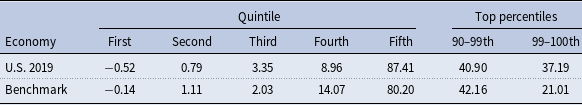
4. Counterfactual policy analysis
We use counterfactual analysis to address several policy-related questions. These include (i) Is a pandemic-era wage subsidy welfare-improving? (ii) What is the optimal wage subsidy schedule? (iii) Under what conditions is the welfare gain from a wage subsidy larger than the welfare gain from a temporary increase in unemployment benefits? (iv) Who gains the most from a wage subsidy? We work through these questions in turn.
4.1 Optimal wage subsidy policy
We seek an optimal combination of wage subsidy parameters $\psi _0$
and
$\psi _0$
and $\overline{\theta }$
that maximize social welfare, taking into account the entire transition path of the economy starting at
$\overline{\theta }$
that maximize social welfare, taking into account the entire transition path of the economy starting at $t=0$
. To put this formally, let
$t=0$
. To put this formally, let $\mathcal{W}(\psi _0,\overline{\theta })$
be social welfare measured by ex-ante utility, specifically:
$\mathcal{W}(\psi _0,\overline{\theta })$
be social welfare measured by ex-ante utility, specifically:
 \begin{align} \mathcal{W}(\psi _0,\overline{\theta }) & = \phi \int _b \int _\theta \sum _{i=\{1,2,3\}} \left( \sum _{s=\{e,u\}} V^A_0 (i,b,\theta,s)g_0^A(i,b,\theta,s)\right.\nonumber\\&\quad \left. + \int _z V^A_0 (i,b,\theta,s,z) \tilde{g}_0^A(i,b,\theta,s,z)dz \right)db d\theta \nonumber\\ & \quad + (1-\phi ) \int _b \int _\theta \left( \sum _{i=\{1,2,3\}} \sum _{s=\{e,u\}} V_0^{UA}(i,b,\theta,s)g_0^{UA}(i,b,\theta,s) \right)db d\theta. \end{align}
Note that the components of $\mathcal{W}(\psi _0,\overline{\theta })$
, namely
$\mathcal{W}(\psi _0,\overline{\theta })$
, namely $V^A_0$
,
$V^A_0$
, $V^{UA}_0$
,
$V^{UA}_0$
, $g^A_0$
,
$g^A_0$
, $\tilde{g}^A_0$
and
$\tilde{g}^A_0$
and $g^{UA}_0$
, as well as the policy parameters
$g^{UA}_0$
, as well as the policy parameters $\psi _0$
and
$\psi _0$
and $\overline{\theta }$
, are all part of the equilibrium defined in Appendix B. The planning problem can then be described as choosing
$\overline{\theta }$
, are all part of the equilibrium defined in Appendix B. The planning problem can then be described as choosing $\psi _0$
and
$\psi _0$
and $\overline{\theta }$
to maximize
$\overline{\theta }$
to maximize $\mathcal{W}(\psi _0,\overline{\theta })$
, subject to the constraint that the choice variables are part of an equilibrium as defined.
$\mathcal{W}(\psi _0,\overline{\theta })$
, subject to the constraint that the choice variables are part of an equilibrium as defined.
In Figure 2, we graph $\mathcal{W}(\psi _0,\overline{\theta })$
, transformed into consumption equivalent variation relative to the “no subsidy” case.Footnote
13
Any wage subsidy within the range that we simulate improves welfare compared to no subsidy. Furthermore, welfare is concave in the both policy parameters, resulting in an interior solution for the optimal policy. Specifically, the optimal wage subsidy scheme is
$\mathcal{W}(\psi _0,\overline{\theta })$
, transformed into consumption equivalent variation relative to the “no subsidy” case.Footnote
13
Any wage subsidy within the range that we simulate improves welfare compared to no subsidy. Furthermore, welfare is concave in the both policy parameters, resulting in an interior solution for the optimal policy. Specifically, the optimal wage subsidy scheme is $\psi _0^*=.85$
with a ceiling
$\psi _0^*=.85$
with a ceiling $\overline{\theta }^*=\$350$
. This policy implies that many matches in which workers earn less than $350/week will be kept during the lockdown, regardless of the productivity of their job, and some higher earning workers will also be retained by their employers. On the other hand, about half of the workers whose salaries are subsidized at
$\overline{\theta }^*=\$350$
. This policy implies that many matches in which workers earn less than $350/week will be kept during the lockdown, regardless of the productivity of their job, and some higher earning workers will also be retained by their employers. On the other hand, about half of the workers whose salaries are subsidized at $t=0$
would have been kept on payroll anyway. The average weekly cost of such redundant subsidization works out to about 0.063
$t=0$
would have been kept on payroll anyway. The average weekly cost of such redundant subsidization works out to about 0.063 $\%$
of steady-state weekly GDP, which limits the scope of the optimal policy.
$\%$
of steady-state weekly GDP, which limits the scope of the optimal policy.
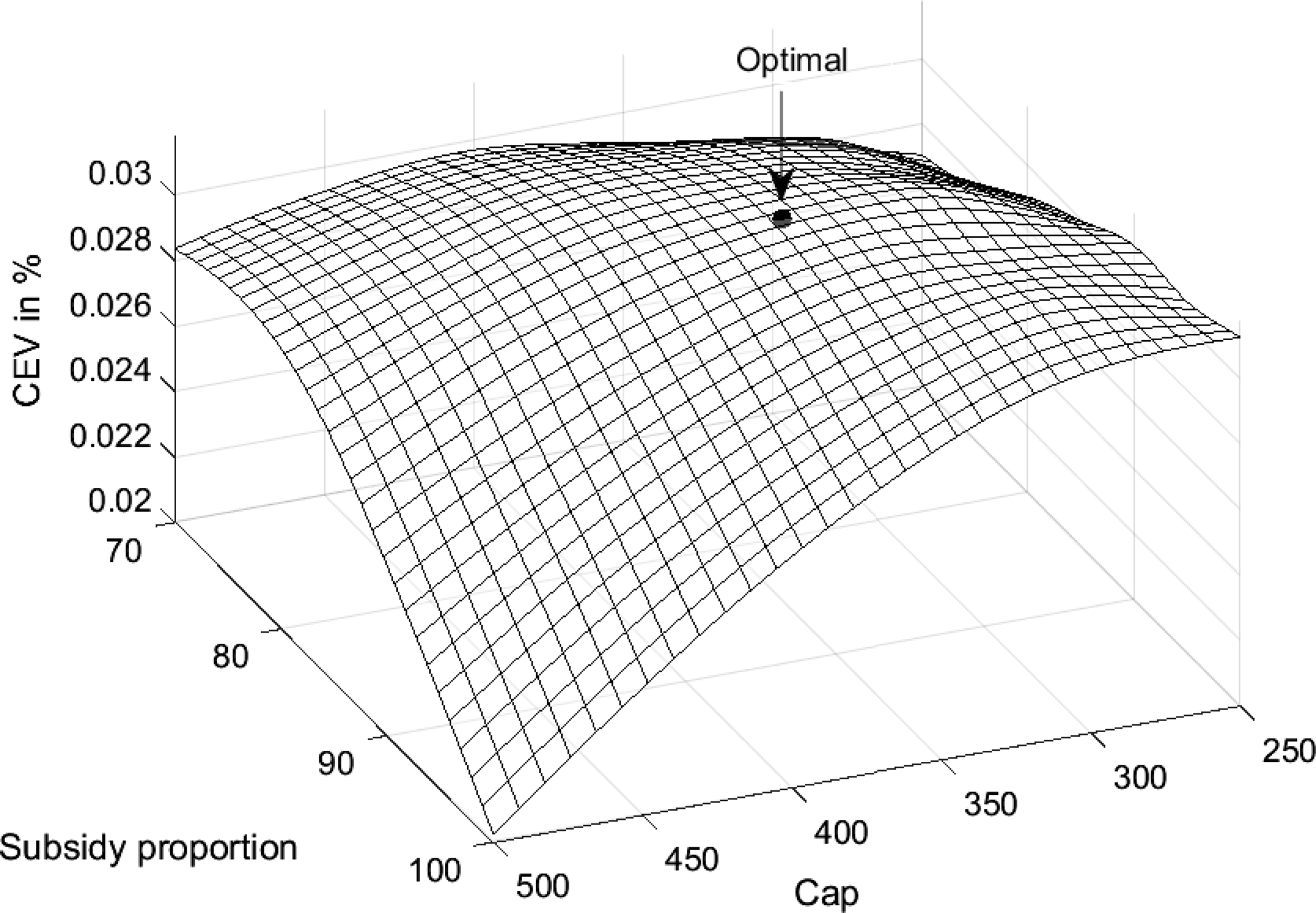
Figure 2. Consumption equivalent variation of various $(\psi _0,\overline{\theta })$
combinations compared to the “no subsidy” scheme. The marginal subsidy rate,
$(\psi _0,\overline{\theta })$
combinations compared to the “no subsidy” scheme. The marginal subsidy rate, $\psi _0$
, is in percentage units. The ceiling,
$\psi _0$
, is in percentage units. The ceiling, $\bar{\theta }$
, is in dollars.
$\bar{\theta }$
, is in dollars.
4.2 UI policy with a ceiling
Instead of offering a wage subsidy, government could increase unemployment insurance benefits in the affected sector (we call this the UI policy). We consider a UI policy that temporarily increases the replacement rate to 100 $\%$
up to a ceiling, which replicates the full salary received by workers under a wage subsidy.Footnote
14
Formally, we solve the model with the following unemployment benefit function:
$\%$
up to a ceiling, which replicates the full salary received by workers under a wage subsidy.Footnote
14
Formally, we solve the model with the following unemployment benefit function:
 \begin{equation} \begin{aligned} \tilde{h}_t(\theta ) = 0.4 \times \theta + \min \left( 0.6 \times \theta, \bar{h} \right), \: 0 \leq t \lt t^{\text{open}}. \end{aligned} \end{equation}
The first term is the benchmark 40 $\%$
replacement, and the second term represents replacing the remaining 60
$\%$
replacement, and the second term represents replacing the remaining 60 $\%$
of salary up to the ceiling
$\%$
of salary up to the ceiling $\bar{h}$
. We compute the CEV associated with various values of
$\bar{h}$
. We compute the CEV associated with various values of $\bar{h}$
and present the result in the Figure 3. The CEV is positive for all ceiling values plotted, and there is a clear optimal ceiling around $275 per week. This is equivalent to fully replacing the income of unemployed workers whose weekly earnings were
$\bar{h}$
and present the result in the Figure 3. The CEV is positive for all ceiling values plotted, and there is a clear optimal ceiling around $275 per week. This is equivalent to fully replacing the income of unemployed workers whose weekly earnings were $\$275$
/week or less, and sending a top-up payment to those who previously earned more.
$\$275$
/week or less, and sending a top-up payment to those who previously earned more.

Figure 3. Consumption equivalent variation of the UI policy with various ceilings compared to the laissez-faire case.
4.3 Wage subsidy versus increased unemployment benefits
The distribution of firm profit margins is a key factor determining the measure of workers kept on payroll versus laid off. When profit margin is higher, the relative value of keeping an affected job increases, which results in fewer endogenous layoffs and a lesser role for a subsidy. Figure 4 plots the welfare gains from optimal wage subsidy and UI policies over a range of mean profit margins. When average profit margin exceeds 12.25%, the UI policy dominates and vice versa. In our benchmark economy, the mean profit margin is 12 $\%$
, so the wage subsidy slightly dominates.
$\%$
, so the wage subsidy slightly dominates.

Figure 4. Consumption equivalent variation of the optimal wage subsidy scheme compared to the UI policy for various means of profit margin. The subsidy rate, $\psi _0$
is in percentage. The ceiling,
$\psi _0$
is in percentage. The ceiling, $\bar{\theta }$
, is in $ term.
$\bar{\theta }$
, is in $ term.
Shutdown duration also influences the value of keeping a job. In the absence of the subsidy, longer shutdown duration presents a longer stream of wage payments that firms have to make to keep workers employed, whereas the future value of the job remains the same. As such, the present value of keeping a worker on payroll will be negatively related to shutdown duration. Figure 5 displays the relative welfare gains of the two types of policy over different shutdown lengths. For any shutdown longer than 11 weeks, the wage subsidy dominates and vice versa.

Figure 5. Consumption equivalent variation of the optimal wage subsidy scheme compared to the UI policy for length of shutdown duration.
We also experimented with varying the size of the affected sector, $\phi$
. While the value of both policies increases with sector size, their ranking is robust to changing this parameter.
$\phi$
. While the value of both policies increases with sector size, their ranking is robust to changing this parameter.
4.4 Jointly optimal wage subsidy and UI enhancement
We now solve for an optimal mixed policy that combines the capped UI policy with the wage subsidy. In particular, we find the set of parameters $\big(\psi _0,\bar{\theta },\bar{h}\big)$
that maximize the welfare function as in (24). The results are illustrated in Figure 6, which plots the welfare gains from the joint policy across several values of the UI ceiling, along with the welfare gains from the respective UI policies absent the wage subsidy. The optimal UI ceiling is again about $275, and the optimal subsidy given this ceiling is 90
$\big(\psi _0,\bar{\theta },\bar{h}\big)$
that maximize the welfare function as in (24). The results are illustrated in Figure 6, which plots the welfare gains from the joint policy across several values of the UI ceiling, along with the welfare gains from the respective UI policies absent the wage subsidy. The optimal UI ceiling is again about $275, and the optimal subsidy given this ceiling is 90 $\%$
capped at $200/week. Thus, although the optimal UI policy is the same as when specified independently, the optimal wage subsidy is different in two ways. First, the subsidy ceiling is much lower, being $200/week, as opposed to $350/week when unemployment benefits are held constant. Second, the marginal subsidy rate is slightly higher when unemployment benefits are also adjusted. Overall, this means that the government offers weaker incentives to keep high earning workers on payroll when UI has been temporarily increased and instead offers income replacement through benefits. This is because the extension of UI allows the policy maker to be more aggressive in avoiding subsidizing high profit jobs that would not have been displaced anyway because they are assured low-income/wealth workers will collect higher unemployment benefits if they lose their jobs as a consequence.
$\%$
capped at $200/week. Thus, although the optimal UI policy is the same as when specified independently, the optimal wage subsidy is different in two ways. First, the subsidy ceiling is much lower, being $200/week, as opposed to $350/week when unemployment benefits are held constant. Second, the marginal subsidy rate is slightly higher when unemployment benefits are also adjusted. Overall, this means that the government offers weaker incentives to keep high earning workers on payroll when UI has been temporarily increased and instead offers income replacement through benefits. This is because the extension of UI allows the policy maker to be more aggressive in avoiding subsidizing high profit jobs that would not have been displaced anyway because they are assured low-income/wealth workers will collect higher unemployment benefits if they lose their jobs as a consequence.

Figure 6. Consumption equivalent variation of the UI policy with various cap compared to the laissez-faire case.
4.5 The role of heterogeneity in policy making
The model features heterogeneity along several dimensions and the shutdown only hits the affected sector; thus, any subsidy policy will naturally lead to redistribution. To determine which income groups gain the most from policy reforms, Figure 7 reports the results of a simple welfare decomposition. For both wage subsidy and UI policies, the welfare gain is decreasing in income. For the lowest income group, the CEVs from wage subsidy and UI policy are about 0.055 $\%$
. For other income groups, the CEV gains from the UI policy are higher than from the wage subsidy. Interestingly, the top income groups see a decrease in welfare under either policy. This is because (1) high-income workers are more likely matched with high-productivity firms, and these firms would more likely retain their workers anyway, (2) high-income workers often have high net worth and thus would be able to smooth consumption during the shutdown, and (3) both policies imply higher future tax rates with similar drops of
$\%$
. For other income groups, the CEV gains from the UI policy are higher than from the wage subsidy. Interestingly, the top income groups see a decrease in welfare under either policy. This is because (1) high-income workers are more likely matched with high-productivity firms, and these firms would more likely retain their workers anyway, (2) high-income workers often have high net worth and thus would be able to smooth consumption during the shutdown, and (3) both policies imply higher future tax rates with similar drops of $\lambda$
to about
$\lambda$
to about $\tilde{\lambda }=0.9012$
, meaning long-run consumption falls by about 0.1
$\tilde{\lambda }=0.9012$
, meaning long-run consumption falls by about 0.1 $\%$
.
$\%$
.

Figure 7. Decomposition of welfare gain from switching from baseline to optimal wage subsidy and UI policy.
4.6 Further robustness checks
Here we report the results of two further robustness checks. The first check was to allow labor supply to respond to the increase in tax rates starting at time $t^{\text{rec}}$
. We implement this in our model by shrinking each worker’s value of
$t^{\text{rec}}$
. We implement this in our model by shrinking each worker’s value of $\theta$
by a fixed percentage. This fixed percentage is calculated by assuming a Frisch labor supply elasticity of 0.5, and using the reduction in net wages associated with the decrease of
$\theta$
by a fixed percentage. This fixed percentage is calculated by assuming a Frisch labor supply elasticity of 0.5, and using the reduction in net wages associated with the decrease of $\lambda$
to
$\lambda$
to $\tilde{\lambda }$
(note that the percentage reduction in net wage is independent of
$\tilde{\lambda }$
(note that the percentage reduction in net wage is independent of $\theta$
). To make this exercise feasible, we assume that labor supply falls permanently at
$\theta$
). To make this exercise feasible, we assume that labor supply falls permanently at $t=0$
, as opposed to
$t=0$
, as opposed to $t^{\text{rec}}$
, because otherwise there would be changes in the values of jobs and vacancies at
$t^{\text{rec}}$
, because otherwise there would be changes in the values of jobs and vacancies at $t^{\text{rec}}$
, leading to further labor market transition. The main consequence of reducing labor supply is that the tax base is smaller in the new steady-state, implying a higher tax rate to pay for pandemic programs. However, the effect of reduced labor supply on taxes is very small, requiring
$t^{\text{rec}}$
, leading to further labor market transition. The main consequence of reducing labor supply is that the tax base is smaller in the new steady-state, implying a higher tax rate to pay for pandemic programs. However, the effect of reduced labor supply on taxes is very small, requiring $\tilde{\lambda }=0.9011$
as opposed to
$\tilde{\lambda }=0.9011$
as opposed to $\tilde{\lambda }=0.9012$
. Similarly, the welfare gain from the optimal wage subsidy is smaller by only 4e-5
$\tilde{\lambda }=0.9012$
. Similarly, the welfare gain from the optimal wage subsidy is smaller by only 4e-5 $\%$
.
$\%$
.
Our final robustness check relates to how the labor market is calibrated. In our calibration, the value of unemployment is quite low compared to employment because the replacement rate is only 40 $\%$
. However, in Hagedorn and Manovskii (Reference Hagedorn and Manovskii2008) the value of unemployment is much higher because of allowing for, example, home production. We check the sensitivity to this by allowing home production equivalent to 50
$\%$
. However, in Hagedorn and Manovskii (Reference Hagedorn and Manovskii2008) the value of unemployment is much higher because of allowing for, example, home production. We check the sensitivity to this by allowing home production equivalent to 50 $\%$
of salary. In this case, it is never optimal to subsidize wages during a pandemic, which makes sense because laid off workers can produce at home. We provide more details on this robustness check in Appendix C.
$\%$
of salary. In this case, it is never optimal to subsidize wages during a pandemic, which makes sense because laid off workers can produce at home. We provide more details on this robustness check in Appendix C.
5. Conclusion
We have contributed a model that captures many relevant margins affecting the efficacy of employment-related policies in a pandemic. The model includes labor market frictions that determine which workers will be laid off in a pandemic-related shut down, and also how quickly laid-off workers will find new jobs after the shut down ends. Wage rigidity in the model implies potentially large increases in the unemployment rate when the pandemic hits. Workers in the least profitable matches are the most likely to be laid off, and assortative matching between worker and job productivity implies that low-income workers will be the hardest hit. The model also features an endogenous distribution of household consumption and wealth. Wealthy households can smooth consumption over the pandemic better than poorer households, which means that low-income workers tend to also suffer the most from a layoff.
We considered wage subsidy and enhanced unemployment benefit policy responses to the economic disruption. Wage subsidies encourage firms to keep workers on payroll, which leads to a much faster labor market recovery after the pandemic ends. However, a wage subsidy program can be fiscally costlier than expanding unemployment benefits, implying a tradeoff. Either policy option is paid for through higher future income tax rates.
We offer several concrete policy conclusions. Either a wage subsidy or enhanced unemployment benefits will reduce the welfare cost of the pandemic. Which of the two policy options is better depends on characteristics of the pre-pandemic economy and the nature of the pandemic. In an economy where the (pre-pandemic) average profit margin of firms is small (less than 12.25 $\%$
), a wage subsidy program will be more beneficial than enhanced unemployment insurance and vice versa. This is because the low profit margins will imply large numbers of layoffs, absent a wage subsidy. Similarly, if the shut down period will be long (more than 11 weeks) then a wage subsidy is better. A long shut down cuts into the profit associated with keeping a worker on payroll, thus leading to large numbers of layoffs like when profit margins are small. Lastly, the most efficacious policy includes both a small wage subsidy and enhanced unemployment benefits. Under the baseline parameters of our model, calibrated to match US data, a wage subsidy covering 90
$\%$
), a wage subsidy program will be more beneficial than enhanced unemployment insurance and vice versa. This is because the low profit margins will imply large numbers of layoffs, absent a wage subsidy. Similarly, if the shut down period will be long (more than 11 weeks) then a wage subsidy is better. A long shut down cuts into the profit associated with keeping a worker on payroll, thus leading to large numbers of layoffs like when profit margins are small. Lastly, the most efficacious policy includes both a small wage subsidy and enhanced unemployment benefits. Under the baseline parameters of our model, calibrated to match US data, a wage subsidy covering 90 $\%$
of the first $200/week of earnings combined with increased unemployment benefits replacing the first $275/week of earnings is optimal. This is in contrast to the US policy response, which expanded UI benefits by $600 per week, but did not include a wage subsidy.
$\%$
of the first $200/week of earnings combined with increased unemployment benefits replacing the first $275/week of earnings is optimal. This is in contrast to the US policy response, which expanded UI benefits by $600 per week, but did not include a wage subsidy.
In closing, it is worth discussing several issues related to our study that we abstract from in our model. First, we do not model interactions between economic policy and disease transmission risk. This is because we take as given that workers in the affected sector cannot work. Thus, subsidizing their salaries keeps them on payroll, but does not change the likelihood of their being infected. Second, we abstract from long-run cleansing effects of recessions. Although jobs that are kept during the pandemic tend to be high-productivity jobs, in the long run the distribution of job productivity returns to steady state. Lastly, because we model wages as fixed, we do not model job-specific human capital. Such a feature would might add an additional layer of benefit to wage subsidies, as a labor market recovery would require not only full employment to be reattained, but also additional worker training. This might lengthen the recovery period, making future tax rates somewhat higher.
Appendix
A. Aggregates
The aggregate unemployment rate is:
 \begin{equation} \begin{aligned} U_t = \phi U_t^A + (1-\phi )U_t^{UA} \end{aligned} \end{equation}
where
 \begin{equation} \begin{aligned} U_t^{UA} =& \sum _i\int _b \int _\theta g_t^{UA}(i,b,\theta,u)dbd\theta \\ U_t^A =& \sum _i\int _b \int _\theta \bigg ( g_t^A(i,b,\theta,u) + \int _z \tilde{g}_t^A(i,b,\theta,a,z)dz \bigg ) dbd\theta \\ \end{aligned} \end{equation}
Next, we define some aggregates that are used to state the government budget constraint above. Aggregate tax revenue in the initial steady state is:
 \begin{equation} \begin{aligned} \mathcal{T} = \sum _i\int _b \int _{\theta } T(\theta ) g(i,b,\theta,e) db d\theta + \sum _i\int _b \int _{\theta } \frac{T(\theta )}{\theta }h(\theta ) g(i,b,\theta,u) db d\theta \end{aligned} \end{equation}
where $T(\theta )/\theta$
is the average tax rate of an individual with salary
$T(\theta )/\theta$
is the average tax rate of an individual with salary $\theta$
. In the final steady state, this becomes:
$\theta$
. In the final steady state, this becomes:
 \begin{equation} \begin{aligned} \tilde{\mathcal{T}} = \sum _i\int _b \int _{\theta } \tilde{T}(\theta ) g^f(i,b,\theta,e) db d\theta + \sum _i\int _b \int _{\theta } \frac{\tilde{T}(\theta )}{\theta }h(\theta ) g^f(i,b,\theta,u) db d\theta \end{aligned} \end{equation}
where $g^f(i,b,\theta,s)$
is the distribution of household state variables in the final steady state. During the pandemic, tax revenue is
$g^f(i,b,\theta,s)$
is the distribution of household state variables in the final steady state. During the pandemic, tax revenue is
 \begin{equation} \begin{aligned} \mathcal{T}_t =\, & \phi \sum _i\int _b \int _{\theta } \int _z T(\theta ) \tilde{g}_t^A(i,b,\theta,e,z) db d\theta dz + (1-\phi ) \sum _i\int _b \int _{\theta } T(\theta ) g_t^{UA}(i,b,\theta,e) db d\theta \\ & + \phi \sum _i\int _b \int _{\theta } \frac{T(\theta )}{\theta }\tilde{h}(\theta ) \left(\int _z \tilde{g}_t^A(i,b,\theta,a,z)dz + g_t^A(i,b,\theta,u)\right) db d\theta \\ & + (1-\phi ) \sum _i\int _b \int _{\theta } \frac{T(\theta )}{\theta }h(\theta ) g_t^{UA}(i,b,\theta,u) db d\theta, \ 0\leq t\lt t^{\text{open}}. \end{aligned} \end{equation}
This simplifies during the recovery period to:
 \begin{equation} \begin{aligned} \mathcal{T}_t = & \sum _i\int _b \int _{\theta } T(\theta ) g_t(i,b,\theta,e) db d\theta \\ & + \sum _i\int _b \int _{\theta } \frac{T(\theta )}{\theta }h(\theta ) g_t(i,b,\theta,u) db d\theta, \ t^{\text{open}}\leq t\lt t^{\text{rec}}. \end{aligned} \end{equation}
In steady state ,the aggregate cost of unemployment benefits is:
 \begin{equation} \begin{aligned} & H = \sum _i\int _b \int _{\theta } h(\theta ) g(i,b,\theta,u) db d\theta \\ \end{aligned} \end{equation}
which is the same in both initial and final steady states, given that the distributions of $\theta$
and
$\theta$
and $s$
are the same in the two steady states. During the pandemic, the aggregate unemployment benefit cost is
$s$
are the same in the two steady states. During the pandemic, the aggregate unemployment benefit cost is
 \begin{equation} \begin{aligned} H_t =\, & \phi \sum _i\int _b \int _{\theta } \tilde{h}(\theta ) \left(\int _z \tilde{g}_t^A(i,b,\theta,a,z)dz+g_t^A(i,b,\theta,u)\right) db d\theta \\ & + (1-\phi ) \sum _i\int _b \int _{\theta } h(\theta ) g_t^{UA}(i,b,\theta,u) db d\theta, \ 0\leq t\lt t^{\text{open}}\\ \end{aligned} \end{equation}
while during the recovery period it is:
 \begin{equation} \begin{aligned} H_t = & \sum _i\int _b \int _{\theta } h(\theta ) g_t(i,b,\theta,u) db d\theta, \ t^{\text{open}}\leq t\lt t^{\text{rec}}. \\ \end{aligned} \end{equation}
During the pandemic, government expenditure on the wage subsidy is:
 \begin{equation} \begin{aligned} & Q_t = \phi \sum _i\int _b \int _\theta \int _z \psi (\theta )\theta \tilde{g}_t^A(i,b,\theta,e,z)dbd\theta dz. \\ \end{aligned} \end{equation}
B. Definition—equilibrium
B.1 Initial steady-state equilibrium
An equilibrium for the initial steady state is a value function $V(i,b,\theta,s)$
and optimal policy functions
$V(i,b,\theta,s)$
and optimal policy functions $c(i,b,\theta,s)$
and
$c(i,b,\theta,s)$
and $\dot{b}(i,b,\theta,s)$
, a probability measure
$\dot{b}(i,b,\theta,s)$
, a probability measure $g(i,b,\theta,s)$
, for
$g(i,b,\theta,s)$
, for $i \in \{1, 2, 3\}$
and
$i \in \{1, 2, 3\}$
and $s \in \{e,u\}$
, and a market tightness
$s \in \{e,u\}$
, and a market tightness $\Theta$
such that
$\Theta$
such that
-
Given market tightness $\Theta$
, the value function
$V(i,b,\theta,s)$
solves the HJB equations (3) and (4), and
$c(i,b,\theta,s)$
and
$\dot{b}(i,b,\theta,s)$
are the associated policy function.
$\Theta$
, the value function
$V(i,b,\theta,s)$
solves the HJB equations (3) and (4), and
$c(i,b,\theta,s)$
and
$\dot{b}(i,b,\theta,s)$
are the associated policy function. -
The market tightness
$\Theta$
satisfies the free-entry condition (8) with
$W=0$
. -
The probably measure follows the KFE equation (5) with
$\dot{g}(i,b,\theta,s)=0$
for
$i \in \{1, 2, 3\}$
and
$s \in \{e,u\}$
.


B.2 Final steady-state equilibrium
An equilibrium for the initial steady state is a value function $V^f(i,b,\theta,s)$
and associated optimal policy functions
$V^f(i,b,\theta,s)$
and associated optimal policy functions $c^f(i,b,\theta,s)$
and
$c^f(i,b,\theta,s)$
and $\dot{b}^f(i,b,\theta,s)$
, a probability measure
$\dot{b}^f(i,b,\theta,s)$
, a probability measure $g^f(i,b,\theta,s)$
, for
$g^f(i,b,\theta,s)$
, for $i \in \{1, 2, 3\}$
and
$i \in \{1, 2, 3\}$
and $s \in \{e,u\}$
, and a market tightness
$s \in \{e,u\}$
, and a market tightness $\Theta ^f$
such that
$\Theta ^f$
such that
-
Given market tightness
$\Theta ^f$
, the value function
$V^f(i,b,\theta,s)$
and associated policy functions
$c^f(i,b,\theta,s)$
and
$\dot{b}^f(i,b,\theta,s)$
solve augmented versions of the HJB equations (3) and (4) where the tax function
$T(y)$
has been replaced by
$\tilde{T}(y)$
that solves the final steady-state government budget constraint (19). -
The market tightness
$\Theta ^f$
satisfies the free-entry condition (8) with
$W=0$
. -
The probably measure follows the KFE equation (5) with
$\dot{g}^f(i,b,\theta,s)=0$
for
$i \in \{1, 2, 3\}$
and
$s \in \{e,u\}$
.


B.3 Pandemic, recovery, and post-recovery equilibrium
Let $\boldsymbol{s}=(i,b,\theta,s)$
be the usual worker state space and
$\boldsymbol{s}=(i,b,\theta,s)$
be the usual worker state space and $\boldsymbol{{s}}^A=(i,b,\theta,s,z)$
be the worker state space if they are in the affected sector during the pandemic phase. An equilibrium of the model is sequences of sector-specific worker value functions
$\boldsymbol{{s}}^A=(i,b,\theta,s,z)$
be the worker state space if they are in the affected sector during the pandemic phase. An equilibrium of the model is sequences of sector-specific worker value functions $\left\{V^A_t( {\boldsymbol{s}}^A ) \right\}_{0\leq t\lt t^{\text{rec}} }$
and
$\left\{V^A_t( {\boldsymbol{s}}^A ) \right\}_{0\leq t\lt t^{\text{rec}} }$
and $\left\{V^{UA}_t( {\boldsymbol{s}} ) \right\}_{0\leq t\lt t^{\text{rec}} }$
, along with optimal policy functions
$\left\{V^{UA}_t( {\boldsymbol{s}} ) \right\}_{0\leq t\lt t^{\text{rec}} }$
, along with optimal policy functions $\big\{c^A_t\big( {\boldsymbol{s}}^A\big),\dot{b}^A_t( {\boldsymbol{s}}^A ) \big\}_{0\leq t\lt t^{\text{rec}}}$
and
$\big\{c^A_t\big( {\boldsymbol{s}}^A\big),\dot{b}^A_t( {\boldsymbol{s}}^A ) \big\}_{0\leq t\lt t^{\text{rec}}}$
and $\big\{c^{UA}_t( {\boldsymbol{s}} ),\dot{b}^{UA}_t( {\boldsymbol{s}} ) \big\}_{0\leq t\lt t^{\text{rec}}}$
; sector-specific job value functions
$\big\{c^{UA}_t( {\boldsymbol{s}} ),\dot{b}^{UA}_t( {\boldsymbol{s}} ) \big\}_{0\leq t\lt t^{\text{rec}}}$
; sector-specific job value functions $\left\{J^A_t(z,\theta )\right\}_{0\leq t\lt t^{\text{open}}}$
and
$\left\{J^A_t(z,\theta )\right\}_{0\leq t\lt t^{\text{open}}}$
and $\left\{J^{UA}_t(z,\theta )\right\}_{0\leq t\lt t^{\text{open}}}$
; sequences of general probability measures
$\left\{J^{UA}_t(z,\theta )\right\}_{0\leq t\lt t^{\text{open}}}$
; sequences of general probability measures $\left\{g_t( {\boldsymbol{s}} ) \right\}_{t\geq t^{\text{rec}}}$
and sector-specific probability measures
$\left\{g_t( {\boldsymbol{s}} ) \right\}_{t\geq t^{\text{rec}}}$
and sector-specific probability measures $\left\{g^A_t( {\boldsymbol{s}}^A )\right\}_{0\leq t\lt t^{\text{rec}}}$
and
$\left\{g^A_t( {\boldsymbol{s}}^A )\right\}_{0\leq t\lt t^{\text{rec}}}$
and $\left\{g^{UA}_t( {\boldsymbol{s}} )\right\}_{0\leq t\lt t^{\text{rec}}}$
; sequences of general market tightness
$\left\{g^{UA}_t( {\boldsymbol{s}} )\right\}_{0\leq t\lt t^{\text{rec}}}$
; sequences of general market tightness $\left \{\Theta _t\right \}_{t\geq t^{\text{rec}}}$
and sector-specific market tightness
$\left \{\Theta _t\right \}_{t\geq t^{\text{rec}}}$
and sector-specific market tightness $\left \{\Theta ^A_t\right \}_{0\leq t\lt t^{\text{rec}}}$
and
$\left \{\Theta ^A_t\right \}_{0\leq t\lt t^{\text{rec}}}$
and $\left \{\Theta ^{UA}_t\right \}_{0\leq t\lt t^{\text{rec}}}$
; government policy functions
$\left \{\Theta ^{UA}_t\right \}_{0\leq t\lt t^{\text{rec}}}$
; government policy functions $\big\{\tilde{T},\tilde{h}(\theta ),\psi (\theta )\big\}$
; and government debt
$\big\{\tilde{T},\tilde{h}(\theta ),\psi (\theta )\big\}$
; and government debt $\left \{B_t\right \}_{0\leq t\leq t^{\text{rec}}}$
, such that, given initial and final steady-state equilibria:
$\left \{B_t\right \}_{0\leq t\leq t^{\text{rec}}}$
, such that, given initial and final steady-state equilibria:
-
Given sequences of market tightness, government policy functions and
$V^f$
, the affected sector value functions
$\left\{V^A_t\left({\boldsymbol{s}}^A\right)\right\}_{0\leq t\lt t^{\text{open}}}$
solve equations (14), (15) and (16), and
$\left\{V^A_t( {\boldsymbol{s}} )\right\}_{t^{\text{open}}\leq t\lt t^{\text{rec}}}$
solve equations (20) and (16).
$\big\{c^A_t\left({\boldsymbol{s}}^A\right),\dot{b}^A_t\left({\boldsymbol{s}}^A\right)\big\}_{0\leq t\lt t^{\text{open}}}$
and
$\big\{c^A_t({\boldsymbol{s}}),\dot{b}^A_t({\boldsymbol{s}})\big\}_{t^{\text{open}}\leq t\lt t^{\text{rec}}}$
are the associated policy functions. -
Given sequences of market tightness, government policy functions and
$V^f$
, the unaffected sector value functions
$\big\{V^{UA}_t( {\boldsymbol{s}} )\big\}_{0\leq t\lt t^{\text{rec}}}$
solve variations of the HJB equations (3) and (4) as described in Sections 2.2.2 and 2.3.2, for example equation (17).
$\big\{c^{UA}_t({\boldsymbol{s}}),\dot{b}^{UA}_t({\boldsymbol{s}})\big\}_{0\leq t\lt t^{\text{rec}}}$
are the associated policy functions. -
Given sequences of market tightness and government policy functions, the affected sector job value function
$\big\{J^A_t(z,\theta )\big\}_{0\leq t\lt t^{\text{open}}}$
solves
$J_t^A(z,\theta )=\max \left \{K_t^A(z,\theta ),L_t^A(z,\theta )\right \}$
where
$K_t^A(z,\theta )$
and
$L_t^A(z,\theta )$
solve equations (11) and (12) given terminal condition
$K_{t^{\text{open}}}^A(z,\theta )=L_{t^{\text{open}}}^A(z,\theta )=J^*(z,\theta )$
. -
Given sequences of market tightness and government policy functions, the unaffected sector job value function
$\{J^{UA}_t(z,\theta )\}_{0\leq t\lt t^{\text{open}}}$
solves equation (6) with
$J_t$
replaced by
$J^{UA}_t$
. -
The affected sector market tightness
$\left \{\Theta ^A_t\right \}_{0\leq t\lt t^{\text{open}}}$
satisfies the free-entry condition
$W^A_t=0$
for all such
$t\in [0,t^{\text{open}})$
, where
$W^A_t$
is defined in the RHS of (13). -
The affected sector market tightness
$\left \{\Theta ^A_t\right \}_{t^{\text{open}}\leq t\lt t^{\text{rec}}}$
satisfies the free-entry condition
$W^A_t=0$
for all such
$t$
, where
$W^A_t$
is defined in the RHS of (8) with
$J$
,
$g$
,
$W$
and
$U$
replaced by
$J_t^{A}$
,
$g_t^{A}$
,
$W_t^A$
and
$U_t^A$
, respectively. -
The unaffected sector market tightness
$\left \{\Theta ^{UA}_t\right \}_{0\leq t\lt t^{\text{open}}}$
satisfies the free-entry condition
$W^{UA}_t=0$
for all such
$t$
, where
$W^{UA}_t$
is defined in the RHS of (8) with
$J$
,
$g$
,
$W$
and
$U$
replaced by
$J_t^{UA}$
,
$g^{UA}$
,
$W_t^{UA}$
and
$U_t^{UA}$
, respectively. -
The general market tightness
$\Theta _t=\Theta ^f$
for all
$t\geq t^{\text{rec}}$
, where
$\Theta ^f$
satisfies the free-entry condition
$W=0$
for all such
$t$
, where
$W$
is defined in the RHS of (8). -
Government debt
$\{B_t\}_{0\leq t\leq t^{\text{rec}}}$
satisfies equation (18) with
$Q_t = 0$
for
$t \geq t^{\text{open}}$
, given
$\psi (\theta )$
,
$\tilde{h}(\theta )$
and
$B_0=0$
. -
The reformed government tax function
$\tilde{T}(y)$
satisfies (19), given the government debt
$B_{t^{\text{rec}}}$
. -
The law-of-motion for the probability measure of unaffected workers for
$t\in [0,t^{\text{rec}})$
is:(36)
\begin{equation} \begin{aligned} \dot{g}_t^{UA}(i,b,\theta,e) = & -\partial _b \big[ \dot{b}^{UA}_t(i,b,\theta,e)g_t^{UA}(i,b,\theta,e) \big] + f^{UA}_t g^{UA}_t(i,b,\theta,u) - \sigma g^{UA}_t(i,b,\theta,e) \\ & + \sum _{j\neq i} \pi _{\rho }\left (g^{UA}(j,b,\theta,e) - g^{UA}(i,b,\theta,e)\right )\\ \dot{g}_t^{UA}(i,b,\theta,u) = &-\partial _b \big[ \dot{b}^{UA}_t(i,b,\theta,u)g_t^{UA}(i,b,\theta,u) \big] - f^{UA}_t g^{UA}_t(i,b,\theta,u) + \sigma g^{UA}_t(i,b,\theta,e) \\ & + \sum _{j\neq i} \pi _{\rho }\left (g^{UA}(j,b,\theta,u) - g^{UA}(i,b,\theta,u)\right ) \end{aligned} \end{equation}
-
The probability measures of affected sector attached-unemployed and employed workers for
$t\in [0,t^{\text{open}})$
satisfy the following conditions, where
$I_t(z,\theta )=\mathcal{I}\left \{K_t(z,\theta )\geq L_t(z,\theta )\right \}$
and
$dI_t(z,\theta )=\mathcal{I}\left \{K_t(z,\theta )\geq L_t(z,\theta )\right \}$
-
$\mathcal{I}\left \{K_{t-dt}(z,\theta )\geq L_{t-dt}(z,\theta )\right \}$
:Footnote
15
(37)for attached-unemployed workers, where
\begin{equation} \begin{array}{rll} \dot{\tilde{g}}_t^{A}(i,b,\theta,a,z) = & F(i,b,\theta,a,z) &{\rm{if}} \ \ I_t(z,\theta ) = 0 \\ \tilde{g}_t^{A}(i,b,\theta,a,z) = & 0 &{\rm{if}} \ \ I_t(z,\theta ) = 1 \end{array} \end{equation}
(38)And for employed workers
\begin{equation} \begin{aligned} F(i,b,\theta,a,z) = &-\partial _b \left[ \dot{{b}}^A_t(i,b,\theta,a,z)\tilde{g}^A_t(i,b,\theta,a,z) \right] \\[3pt] & - \left(\varphi +f^A_t P_z(z|\theta ) \mathcal{I}\{K_t(z,\theta ) \geq 0 \}\right) \tilde{g}_t^A(i,b,\theta,a,z) \\[3pt] & + \sum _{j\neq i} \pi _{\rho }\left (\tilde{g}^{A}(j,b,\theta,a,z) - \tilde{g}^{A}(i,b,\theta,a,z)\right ). \end{aligned} \end{equation}
(39)where
\begin{equation} \begin{array}{rll} \dot{\tilde{g}}_t^{A}(i,b,\theta,e) = & \tilde{F}(i,b,\theta,e) & \forall \ t \in [0,t^{\text{open}}) \\ \tilde{g}_t^{A}(i,b,\theta,e) = & \tilde{g}_{t-dt}^{A}(i,b,\theta,a,z) + \tilde{g}_{t-dt}^{A}(i,b,\theta,e)+\dot{\tilde{g}}_{t-dt}^{A}(i,b,\theta,e)\cdot dt &{\rm{if}} \ \ dI_t(z,\theta )= 1, \forall z \end{array} \end{equation}
(40)
\begin{align} F(i,b,\theta,e) &= -\partial _b \left[ \dot{{b}}^A_t(i,b,\theta,e)\tilde{g}_t^{A}(i,b,\theta,e) \right] \nonumber\\[3pt] & + f^A_t \int _zP_z(z|\theta ) \mathcal{I}\{K_t(z,\theta ) \geq 0 \}dz \bigg (\int _{\tilde{z}} \tilde{g}_t^A(i,b,\theta,a,\tilde{z})d\tilde{z} + g_t^A(i,b,\theta,u) \bigg ) \nonumber\\[3pt] & - \sigma \tilde{g}_t^{A}(i,b,\theta,e) \nonumber\\[3pt] & + \sum _{j\neq i} \pi _{\rho }\left (\tilde{g}^{A}(j,b,\theta,e) - \tilde{g}^{A}(i,b,\theta,e)\right ). \end{align}
-
The law-of-motion for the probability measure of affected sector unattached-unemployed workers for
$t\in [0,t^{\text{open}})$
satisfies:(41)
\begin{equation} \begin{aligned} \dot{g}_t^{A}(i,b,\theta,u) =& -\partial _b \left[ \dot{b}^A_t(i,b,\theta,u)g^{A}_t(i,b,\theta,u) \right] \\[4pt] & - \bigg (f^A_t \int _z P_z(z|\theta ) \mathcal{I}\{ K_t(z,\theta ) \geq 0 \} dz\bigg ) g^{A}_t(i,b,\theta,u) \\[4pt] & + \varphi \int _{\tilde{z}} \tilde{g}^{A}_t(i,b,\theta,a,\tilde{z}) d\tilde{z} \\[4pt] & + \sigma \int _{\tilde{z}} \tilde{g}^{A}_t(i,b,\theta,e,\tilde{z}) d\tilde{z} \\[4pt] & + \sum _{j\neq i} \pi _{\rho }\left (g^{A}(j,b,\theta,u) - g^{A}(i,b,\theta,u)\right ) \end{aligned} \end{equation}
-
The law-of-motion for workers in the affected sector for
$t\in [t^{\text{open}},t^{\text{rec}})$
satisfies:(42)
\begin{equation} \begin{aligned} \dot{g}_t^{A}(i,b,\theta,e) = & -\partial _b \left[ \dot{b}^{A}_t(i,b,\theta,e)g_t^{A}(i,b,\theta,e) \right] + f^{A}_t g^{A}_t(i,b,\theta,u) - \sigma g^{A}_t(i,b,\theta,e) \\ & + \sum _{j\neq i} \pi _{\rho }\left (g^{A}(j,b,\theta,e) - g^{A}(i,b,\theta,e)\right )\\ \dot{g}_t^{A}(i,b,\theta,u) = &-\partial _b \left[ \dot{b}^{A}_t(i,b,\theta,u)g_t^{A}(i,b,\theta,u) \right] - f^{A}_t g^{A}_t(i,b,\theta,u) + \sigma g^{A}_t(i,b,\theta,e) \\ & + \sum _{j\neq i} \pi _{\rho }\left (g^{A}(j,b,\theta,u) - g^{A}(i,b,\theta,u)\right ) \end{aligned} \end{equation}
-
$\underset{t\rightarrow \infty }{\lim }g_t=g^f$
, and the law-of-motion for all workers for
$t\in [t^{\text{rec}},\infty )$
satisfies:(43)
\begin{equation} \begin{aligned} \dot{g}_t(i,b,\theta,e) = & -\partial _b \left[ \dot{b}^f(i,b,\theta,e)g_t(i,b,\theta,e) \right] + f g_t(i,b,\theta,u) - \sigma g_t(i,b,\theta,e) \\ & + \sum _{j\neq i} \pi _{\rho }\left (g(j,b,\theta,e) - g(i,b,\theta,e)\right )\\ \dot{g}_t(i,b,\theta,u) = &-\partial _b \left[ \dot{b}^f(i,b,\theta,u)g_t(i,b,\theta,u) \right] - f g_t(i,b,\theta,u) + \sigma g_t(i,b,\theta,e) \\ & + \sum _{j\neq i} \pi _{\rho }\left (g(j,b,\theta,u) - g(i,b,\theta,u)\right ) \end{aligned} \end{equation}


C. Robustness check—the value of outside option
Hagedorn and Manovskii (Reference Hagedorn and Manovskii2008) argue that the value of outside option of unemployed workers is much higher than the standard calibration, amounting to 0.955. The outside option includes not only the unemployment benefit but also home production or leisure. We perform a robustness check along this line by assuming that the income of unemployed workers consists of two parts: a replacement rate of 40 $\%$
paid by the government and home production valued at 55
$\%$
paid by the government and home production valued at 55 $\%$
of the employment income. Both sources are taxed according to the HSV tax function; however, the revenue from the home production is not used to fund the benefit programs. We make this assumption to ensure that the government debt in the robustness check is similar to the baseline mode and so is the increase in taxes. We then solve the model for several combination of wage subsidy and compute the associated CEV. We present the result in Table 3. The CEV is negative for all considered combinations of wage subsidy parameters. This result makes sense because securing employment income for workers in the affected sector is the primary benefit of the wage subsidy; however, with such a high value of outside options workers would have preferred being laid off and enjoy a higher future consumption that they would have otherwise if they had paid for the wage subsidy.
$\%$
of the employment income. Both sources are taxed according to the HSV tax function; however, the revenue from the home production is not used to fund the benefit programs. We make this assumption to ensure that the government debt in the robustness check is similar to the baseline mode and so is the increase in taxes. We then solve the model for several combination of wage subsidy and compute the associated CEV. We present the result in Table 3. The CEV is negative for all considered combinations of wage subsidy parameters. This result makes sense because securing employment income for workers in the affected sector is the primary benefit of the wage subsidy; however, with such a high value of outside options workers would have preferred being laid off and enjoy a higher future consumption that they would have otherwise if they had paid for the wage subsidy.
Table 3. CEV from the wage subsidy when the value of outside option is worth 95.55 $\%$
of the employed income
$\%$
of the employed income
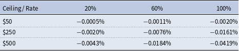
D. Distribution of individual skill
$\theta$

We use data from the March 2019 Current Population Survey Annual Social and Economic Supplement (CPS). We choose this period as it is the nearest date prior to the COVID-19 pandemic, that is the 2020 supplement may include some effects from the pandemic. To construct weekly wages, we divide annual earnings by the number of weeks worked. We then compute the mean and variance of log-weekly earnings, including only those between the ages of 21 and 65.
E. Details of algorithm
E.1 Solving the steady-state HJB equation
The model is solved using a finite-difference method proposed by Achdou et al. (Reference Achdou, Han, Lasry, Lions and Moll2017). Besides the computational advantage of this formulation, the continuous-time model adds an extra element of realism that captures the job-search process in the real world: in discrete-time models households have to wait for one period (for example, one period is 6 weeks in KMS) to find a job. In the continuous-time model, conditional on the same job-finding probability as in the discrete-time counterpart, households will have a good chance to find a job in a short lapse of time.Footnote 16 This difference also between discrete and continuous-time formulation also affects the precautionary motive of households, which is an important aspect that we would like to capture when studying the household welfare under different policy designs.
We discretize the state space into a fine grid and then approximate the value functions at a discrete points in the grid. We first discuss how to solve the initial steady-state HJB equation (3), which is the same for both sectors. Let $b_i, i = 1,\ldots,I$
denote the discrete point in the asset dimension. We use a non-uniform grid and concentrate more points on the bottom part of the asset grid where most of the concavity arises. Let
$b_i, i = 1,\ldots,I$
denote the discrete point in the asset dimension. We use a non-uniform grid and concentrate more points on the bottom part of the asset grid where most of the concavity arises. Let $\rho _j$
denotes the time preference with
$\rho _j$
denotes the time preference with $j \in \{1,2,3\}$
. Let
$j \in \{1,2,3\}$
. Let $\Lambda _{s,s^{\prime}}$
denote the Poisson rate of switching from state
$\Lambda _{s,s^{\prime}}$
denote the Poisson rate of switching from state $s$
to
$s$
to $s^{\prime}$
. For example, if
$s^{\prime}$
. For example, if $s = e$
then
$s = e$
then $s^{\prime} = u$
, and
$s^{\prime} = u$
, and $\Lambda _{s,s^{\prime}} = \sigma$
, that is the job separation rate. Let
$\Lambda _{s,s^{\prime}} = \sigma$
, that is the job separation rate. Let $\theta _{k}, k = 1,\ldots,K$
denote the discrete point in the skill dimension. Denote the argument of a function by the subscript. For example,
$\theta _{k}, k = 1,\ldots,K$
denote the discrete point in the skill dimension. Denote the argument of a function by the subscript. For example, $V_{i,s,j}$
is
$V_{i,s,j}$
is $V(b_i,s,\rho _j)$
, that is the value function at each discrete point in the state space. Let
$V(b_i,s,\rho _j)$
, that is the value function at each discrete point in the state space. Let $y_{s}$
denote the after-tax labor/unemployment benefit income, which only depends on the labor status. We suppress the dependence of value function on
$y_{s}$
denote the after-tax labor/unemployment benefit income, which only depends on the labor status. We suppress the dependence of value function on $\theta$
, with the understanding that
$\theta$
, with the understanding that $\theta$
will enter the value function through labor income and unemployment benefit. The discretized steady-state HJB equation is:
$\theta$
will enter the value function through labor income and unemployment benefit. The discretized steady-state HJB equation is:
 \begin{equation} \begin{aligned} \rho _j V_{i,s,j} =\, & u(c_{i,s,j}) + \underset{\partial _b V_{i,s,j}^F}{ \underbrace{\dfrac{V_{i+1,s,j} - V_{i,s,j}}{\Delta b} }} \big[\dot{b}_{i,s,j}\big]^+ + \underset{\partial _b V_{i,s,j}^B }{ \underbrace{ \dfrac{V _{i,s,j} - V_{i-1,s,j}}{\Delta b} }} \big[\dot{b}_{i,s,j}\big]^- + \Lambda _{s,s^{\prime}} \left[ V_{i,s^{\prime},j} - V_{i,s,j} \right] \\ & + \sum _{h \neq j } \pi _\rho \left[V_{i,s,h} - V_{i,s,j}\right] \end{aligned} \end{equation}
where for any x we have $[x]^+ = \max (0,x)$
and
$[x]^+ = \max (0,x)$
and $[x]^- = \min (0,x)$
. The upwind scheme means if the asset drift is positive then we will use a forward difference, and if the asset drift is negative, we will use a backward difference. Otherwise, if the drift is zero, that is we are in the steady state, the central difference will be used.
$[x]^- = \min (0,x)$
. The upwind scheme means if the asset drift is positive then we will use a forward difference, and if the asset drift is negative, we will use a backward difference. Otherwise, if the drift is zero, that is we are in the steady state, the central difference will be used.
The FOC for (3) is $u^{\prime}(c) = \partial _b V \iff c = (\partial _b V)^{-\frac{1}{\gamma }}$
for the CRRA utility function, and it is held everywhere. As suggested by Achdou et al. (Reference Achdou, Han, Lasry, Lions and Moll2017), the borrowing constraint is replaced by a state constraint boundary condition:
$u^{\prime}(c) = \partial _b V \iff c = (\partial _b V)^{-\frac{1}{\gamma }}$
for the CRRA utility function, and it is held everywhere. As suggested by Achdou et al. (Reference Achdou, Han, Lasry, Lions and Moll2017), the borrowing constraint is replaced by a state constraint boundary condition:
 \begin{equation} \begin{aligned} V_{s,j}(\underline{b}) \geq u^{\prime}(y_s + r \underline{b}), \forall s,j \end{aligned} \end{equation}
Now, define the consumption policy associated with the positive, negative, and no drift as follows:
 \begin{equation} \begin{aligned} & c_{i,s,j}^{F} = \left(\partial _b V_{i,s,j}^F\right)^{-\frac{1}{\gamma }} \\ & c_{i,s,j}^{B} = \left(\partial _b V_{i,s,j}^B\right)^{-\frac{1}{\gamma }} \\ & c_{i,s,j}^{o} = y_s + r b_i \end{aligned} \end{equation}
where the last equation is derived from the budget constraint with $\dot{b} = 0$
. The saving decisions in turns are:
$\dot{b} = 0$
. The saving decisions in turns are:
 \begin{equation} \begin{aligned} & \dot{b}_{i,s,j}^F = y_{s} - r b_i - c_{i,s,j}^F \\ & \dot{b}_{i,s,j}^B = y_{s} - r b_i - c_{i,s,j}^B \\ \end{aligned} \end{equation}
The final consumption policy using the upwind scheme is as follows:
 \begin{equation} \begin{aligned} c_{i,s,j} = \dot{c}_{i,s,j}^F \mathcal{I}\left\{ b_{i,s,j}^F \gt 0 \right\} + \dot{c}_{i,s,j}^B \mathcal{I}\left\{ \dot{b}_{i,s,j}^B \lt 0 \right\} + c_{i,s,j}^0 \mathcal{I} \left\{\dot{b}_{i,s,j}^F \lt 0 \lt \dot{b}_{i,s,j}^B\right\} \end{aligned} \end{equation}
where the last term is derived from the fact that since $V$
is concave in
$V$
is concave in $b$
we have:
$b$
we have:
 \begin{equation} \begin{aligned} \partial _b V_{i,s,j}^F \lt \partial _b V_{i,s,j}^B \implies \dot{b}_{i,s,j}^F \lt \dot{b}_{i,s,j}^B \end{aligned} \end{equation}
which gives us three distinct cases listed above.
Let $n$
index the iterations of the value function. HJB in the matrix form, using an implicit method, is:
$n$
index the iterations of the value function. HJB in the matrix form, using an implicit method, is:
 \begin{equation} \begin{aligned} \dfrac{{\boldsymbol{V}}^{n+1} - {\boldsymbol{V}}^{n} }{\Delta } + \boldsymbol{\rho } {\boldsymbol{V}}^{n+1} & = u({\boldsymbol{c}}^n) + ({\boldsymbol{B}}^n + \boldsymbol{\Lambda }^n + \boldsymbol{\Pi }){\boldsymbol{V}}^n \\ \iff {\boldsymbol{V}}^{n+1} & = \bigg [ \dfrac{1}{\Delta } {\boldsymbol{I}} + \boldsymbol{\rho } - {\boldsymbol{B}}^n - \boldsymbol{\Lambda }^n - \boldsymbol{\Pi } \bigg ]^{-1} \bigg ( u({\boldsymbol{c}}^n) + \dfrac{1}{\Delta } {\boldsymbol{V}}^n \bigg ) \end{aligned} \end{equation}
Here, ${\boldsymbol{I}}$
is an identity matrix of size
${\boldsymbol{I}}$
is an identity matrix of size $I\times 2\times 3\times K$
,
$I\times 2\times 3\times K$
, $\boldsymbol{\rho }$
is a vector stacking
$\boldsymbol{\rho }$
is a vector stacking $[\rho _1, \rho _2, \rho _3]$
,
$[\rho _1, \rho _2, \rho _3]$
, ${\boldsymbol{c}}$
is a vector stacking the optimal consumption policy,
${\boldsymbol{c}}$
is a vector stacking the optimal consumption policy, ${\boldsymbol{V}}$
is a vector stacking the value function, and
${\boldsymbol{V}}$
is a vector stacking the value function, and ${\boldsymbol{B}}^n$
captures the transition along the asset dimension, and it is defined as:
${\boldsymbol{B}}^n$
captures the transition along the asset dimension, and it is defined as:
 \begin{equation} \begin{aligned} {\boldsymbol{B}} = \begin{bmatrix} {\boldsymbol{B}}_{e,j} & \quad \boldsymbol{0} \\[3pt] 0 & \quad {\boldsymbol{B}}_{u,j} \end{bmatrix} \end{aligned} \end{equation}
and for $s \in \{e,u\}$
and
$s \in \{e,u\}$
and $j \in \{1,2,3\}$
:
$j \in \{1,2,3\}$
:
 \begin{equation} \begin{aligned} {\boldsymbol{B}}_{s,j} = \begin{bmatrix} y_{1,s,j} &\quad \upsilon _{1,s,j} &\quad 0 &\quad 0 &\quad \cdots &\quad 0 \\[3pt] x_{2,s,j} &\quad y_{2,s,j} &\quad \upsilon _{2,s,j} &\quad 0 &\quad \cdots &\quad 0 \\[3pt] 0 &\quad x_{3,s,j} &\quad y_{3,s,j} &\quad \upsilon _{3,s,j} &\quad \cdots &\quad 0 \\[3pt] \vdots &\quad \ddots &\quad \ddots &\quad \ddots &\quad \ddots &\quad \vdots \\[3pt] 0 &\quad 0 &\quad 0 &\quad 0 &\quad x_{I,s,j} &\quad y_{I,s,j} \end{bmatrix} \end{aligned} \end{equation}
where:
 \begin{equation} \begin{aligned} &x_{i,s,j} = - \dfrac{ \big[\dot{b}_{i,s,j}\big]^- }{\Delta b} \\[3pt] &\upsilon _{i,s,j} = - \dfrac{ \big[\dot{b}_{i,s,j}\big]^+ }{\Delta b} \\[3pt] &y_{i,s,j} = - x_{i,s,j} - \upsilon _{i,s,j} \end{aligned} \end{equation}
The intuition is that in continuous time, workers can only change its asset position by the size amounting to one step in the asset grid. An implication of this is that the matrix ${\boldsymbol{B}}^n$
is very sparse.
${\boldsymbol{B}}^n$
is very sparse. $\boldsymbol{\Lambda }^n$
captures the transition along employment status dimension, and it is defined as follows:
$\boldsymbol{\Lambda }^n$
captures the transition along employment status dimension, and it is defined as follows:
 \begin{equation} \begin{aligned} \boldsymbol{\Lambda }^n = \begin{bmatrix} -\boldsymbol{\sigma } & \quad \boldsymbol{\sigma } \\ {\boldsymbol{f}} & \quad -{\boldsymbol{f}} \end{bmatrix} \end{aligned} \end{equation} $\boldsymbol{\Pi }$
captures the transition along the time preference dimension:
$\boldsymbol{\Pi }$
captures the transition along the time preference dimension:
 \begin{equation} \begin{aligned} \boldsymbol{\Pi } = \begin{bmatrix} -2\boldsymbol{\pi } &\quad \boldsymbol{\pi } &\quad \boldsymbol{\pi } \\[3pt] \boldsymbol{\pi } &\quad -2\boldsymbol{\pi } &\quad \boldsymbol{\pi } \\[3pt] \boldsymbol{\pi } &\quad \boldsymbol{\pi } &\quad -2\boldsymbol{\pi } \end{bmatrix} \end{aligned} \end{equation}
where the transition rate from $\rho _j$
to
$\rho _j$
to $\rho _h$
is the same for any
$\rho _h$
is the same for any $h \neq j$
.
$h \neq j$
.
Finally, since $\theta$
is fixed skilled, there is no transition along this dimension.
$\theta$
is fixed skilled, there is no transition along this dimension.
With any initial guess $V_{i,s,j}^n$
, iterating the equation (50) will eventually result in a convergence, that is
$V_{i,s,j}^n$
, iterating the equation (50) will eventually result in a convergence, that is $ \lim _{n \rightarrow \infty } \max || V_{i,s,j}^{n+1} - V_{i,s,j}^n|| = 0$
. The intuition is that starting from any value function, if workers experience through the asset accumulation and labor uncertainty for long enough then their decision-making will eventually be stationary. Also, the sparsity of transition matrix implies that such iterating method could be solved very efficiently in a matrix-oriented language (e.g. Matlab).
$ \lim _{n \rightarrow \infty } \max || V_{i,s,j}^{n+1} - V_{i,s,j}^n|| = 0$
. The intuition is that starting from any value function, if workers experience through the asset accumulation and labor uncertainty for long enough then their decision-making will eventually be stationary. Also, the sparsity of transition matrix implies that such iterating method could be solved very efficiently in a matrix-oriented language (e.g. Matlab).
E.2 Solving the transitional-dynamics HJB equation
We first discuss how to solve the sequence of value functions for unaffected sector. The only variable that generate the dynamics in the choice of unaffected workers is the future labor tax. Let $V_{i,s,j}^n = V(b_i,s,\rho _j,t^n)$
, where
$V_{i,s,j}^n = V(b_i,s,\rho _j,t^n)$
, where $t^n$
is the discrete point in time space. The transitional-dynamics HJB equation is:
$t^n$
is the discrete point in time space. The transitional-dynamics HJB equation is:
 \begin{equation} \begin{aligned} \rho _j V_{i,s,j}^n \,=\, &u\big(c_{i,s,j}^{n}\big) + \underset{\partial _b V_{i,s,j}^F}{ \underbrace{\dfrac{V_{i+1,s,j}^n - V_{i,s,j}^n}{\Delta b} }} \big[\dot{b}^n_{i,s,j}\big]^+ + \underset{\partial _b V_{i,s,j}^B }{ \underbrace{ \dfrac{V_{i,s,j}^n - V_{i-1,s,j}^n}{\Delta b} }} \big[\dot{b}^n_{i,s,j}\big]^- \\ & + \Lambda _{s,s^{\prime}} \left[ V_{i,s^{\prime},j}^n - V_{i,s,j}^n \right] + \sum _{h \neq j } \pi _\rho \left[V_{i,s,h} - V_{i,s,j}\right] + \underset{ \partial _t V_{i,s,j} }{ \underbrace{ \dfrac{ V_{i,s,j}^{n+1} - V_{i,s,j}^n }{\Delta t^n} } } \end{aligned} \end{equation}
where the optimal policy functions are time-variant is now also a function of the taxation scheme. In particular:
 \begin{equation} \begin{aligned} \dot{b}_{i,s,j}^n = y_s(\tau ^n) - r b_i^n - c_{i,s_j}^n \end{aligned} \end{equation}
where the policy dependence of optimal policy is captured in $y_s(\tau ^n)$
which depends on time. We solve this HJB equation backward, starting from the terminal stationary value function
$y_s(\tau ^n)$
which depends on time. We solve this HJB equation backward, starting from the terminal stationary value function $V^N_{i,s_j}$
that solves the (44) with the reformed federal tax
$V^N_{i,s_j}$
that solves the (44) with the reformed federal tax $\tilde{\tau }$
in place. The transitional-dynamics HJB equation in the matrix form, using an implicit method, is:
$\tilde{\tau }$
in place. The transitional-dynamics HJB equation in the matrix form, using an implicit method, is:
 \begin{equation} \begin{aligned} {\boldsymbol{V}}^n = \bigg [ \dfrac{1}{\Delta } {\boldsymbol{I}} + \boldsymbol{\rho } - {\boldsymbol{B}}^n - \boldsymbol{\Lambda }^n - \boldsymbol{\Pi } \bigg ]^{-1} \bigg ( u({\boldsymbol{c}}^n) + \dfrac{1}{\Delta } {\boldsymbol{V}}^{{n+1}} \bigg ) \end{aligned} \end{equation}
There are two differences between (50) and (58). First, the time-variant parameters show up in the latter but not the former. Second, the time index is reversed (notice the blue highlight). Intuitively, in the transitional dynamics we know the end value function, and we iterate from that and goes backward to the “current time.” In the steady-state equilibrium, we do not know what the end point is; thus, we iterate from any guess of the value function and go forward until we reach the steady-state.
We now turn to solve the sequence of value functions for affected sector. The labor status is now $s \in \{z,u\}$
. Let
$s \in \{z,u\}$
. Let $z_j,j = 1,\ldots,J$
be the discrete point in the job-specific productivity space. The main difference between this problem and the unaffected workers problem is that workers can be in multiple employment states: (1) employed at job z, (2) attached-unemployed with job z, and (3) unemployed. The transition matrix along the labor status dimension is:
$z_j,j = 1,\ldots,J$
be the discrete point in the job-specific productivity space. The main difference between this problem and the unaffected workers problem is that workers can be in multiple employment states: (1) employed at job z, (2) attached-unemployed with job z, and (3) unemployed. The transition matrix along the labor status dimension is:
 \begin{equation} \begin{aligned} \boldsymbol{\Lambda }^n = \begin{bmatrix} {\boldsymbol{EE}} &\quad {\boldsymbol{EA}} &\quad {\boldsymbol{EU}}\\[3pt] {\boldsymbol{AE}} &\quad {\boldsymbol{AA}} &\quad {\boldsymbol{AU}} \\[3pt] {\boldsymbol{UE}} &\quad {\boldsymbol{UA}} &\quad {\boldsymbol{UU}} \\[3pt] \end{bmatrix} \end{aligned} \end{equation}
where ${\boldsymbol{EU}}$
is a matrix describing the employment-unemployment transition and so forth. These submatrice describes the law-of-motion as laid down in (40), (38), and (41).
${\boldsymbol{EU}}$
is a matrix describing the employment-unemployment transition and so forth. These submatrice describes the law-of-motion as laid down in (40), (38), and (41).
E.3 Characterizing the law-of-motion of the probability measure
As shown in Achdou et al. (Reference Achdou, Han, Lasry, Lions and Moll2017), the law-of-motion for the probability measure $g$
can be characterized by the following KFE:
$g$
can be characterized by the following KFE:
 \begin{equation} \begin{aligned} \dot{g}_t = \left[ {\boldsymbol{B}}^n + \boldsymbol{\Lambda }^n + \boldsymbol{\Pi }\right]^\top g_t \end{aligned} \end{equation}
where the transition matrix is time-independent if we solve for the steady state, and it is time-dependent if we solve for the transitional dynamics. In the steady state, $\dot{{\boldsymbol{g}}}_t = 0$
and thus
$\dot{{\boldsymbol{g}}}_t = 0$
and thus
 \begin{equation} \begin{aligned} 0 = \left[ {\boldsymbol{B}} + \boldsymbol{\Lambda } + \boldsymbol{\Pi }\right]^\top g \end{aligned} \end{equation}
Once we construct ${\boldsymbol{B}}$
and
${\boldsymbol{B}}$
and $\boldsymbol{\Lambda }$
for the HJB, we get the stationary distribution almost for free.Footnote
17
We then paste the distribution of
$\boldsymbol{\Lambda }$
for the HJB, we get the stationary distribution almost for free.Footnote
17
We then paste the distribution of $\theta$
into
$\theta$
into $g$
and rescale so that it integrates to one. When we compute the aggregate variables along the transitional dynamics, we use the stationary measure associated with the initial steady state to initialize the chain (60).
$g$
and rescale so that it integrates to one. When we compute the aggregate variables along the transitional dynamics, we use the stationary measure associated with the initial steady state to initialize the chain (60).


 Open access