


1. Introduction
In this paper, we investigate the impacts of fiscal policy (the dividend, corporate, and bond income taxes) and monetary policy (the nominal interest rate) in an endogenous growth model of R&D. We endogenize the firm’s financial structure (in terms of internal and external funds) and enable the financial market (the equity market and the bond market) to reshuffle loanable funds out of less productive firms toward others with greater productivity. The endogenous financing of R&D provides a potentially important channel to link finance and economic growth. We show that the financial structure-growth relationship is not monotonic and that it depends on the relative productivity between the existing and new firms and the allocation of loanable funds between them. Distinct policies end up with quite different consequences for firms’ financial structures (the demand for loanable funds) and households’ asset investments (the supply of loanable funds), with both jointly determining inflation, growth, and the market structure. High growth can be associated with either an intensive (a large number of firms with a small firm size) or extensive margin (a small number of firms with a large firm size) in terms of market structure.
It is crucial to highlight R&D firms’ financial sources as we examine firms’ innovation activities and their influences on the economy’s performance. It is well documented that innovation activities require a lot of funding, but it is difficult for firms to raise sufficient R&D funds (Schumpeter (Reference Schumpeter1942), ch.VIII), leading to an underinvestment in R&D (Arrow (Reference Arrow1962)). There are two main reasons for this phenomenon: the knowledge nonrivalry and the return divergence between the supply of and demand for funding. Knowledge is nonrivalrous, and this externality gives rise to a disincentive effect, discouraging firms from collecting enough funds for the R&D investment, particularly when they need to raise funds externally.Footnote 1 This calls for the government’s intervention via a patent system (e.g. Segerstrom (Reference Segerstrom2000); Futagami and Iwaisako (Reference Futagami and Iwaisako2007); Iwaisako and Futagami (Reference Iwaisako and Futagami2013); Yang (Reference Yang2018); Chu et al. (Reference Chu, Lai and Liao2019)) or tax incentives (Chu and Cozzi (Reference Chu and Cozzi2018)) to remedy the underinvestment in R&D. Tax incentives may be more attractive to policymakers; for example, corporate taxes have been lowered in many industrial countries. From 1980 to 2018, the average worldwide statutory corporate income tax rate declined from 38.84% to 23.03%, representing a 41% reduction over the past 38 years. Corporate income tax rates declined the most in Europe, decreasing by 55% from 40.5% in 1980 to 18.38% in 2018.
These interventions, however, still have difficulty increasing the availability of external finance. The problem of return divergence, as stressed by Arrow (Reference Arrow1962) and other financial economists, manifests itself when R&D firms do not have enough internal funding (retained earnings) to finance their innovation activities, while external funding is costly. Corporate investment decisions may be distorted because the loanable funds suppliers (households) and demanders (R&D firms) have different objectives and different expectations regarding their returns on R&D.Footnote 2 Conventional R&D growth models ignore the importance of financial structures by simply assuming that firms have enough internal funds (retained earnings) to finance R&D expenditures without the need for external funds. Instead, this study endogenizes firms’ financial structures by considering the return divergence between the supply of and demand for R&D funding. Due to the costly nature of state verification, the agency cost between the supply of and demand for funding exists, giving rise to the return divergence (Jensen and Meckling (Reference Jensen and Meckling1976); Bernanke and Gertler (Reference Bernanke and Gertler1989)). The existence of return divergence vividly portrays the transformation from firms’ external finance to their productivity, which provides a microfoundation of macroeconomics (Carlstrom and Fuerst (Reference Carlstrom and Fuerst1997)). Our analysis accounts for the agency cost and, accordingly, endogenizes R&D firms’ financial structures (specifically, the financial leverage (measured by the debt-equity ratio) and the user cost of capital (measured by the weighted average cost of capital, WACC)). The financial structure of R&D firms will affect the demand for and supply of loanable funds, which in turn governs the effects of fiscal and monetary policy. Thus, we offer quite different policy implications from the conventional wisdom gleaned from growth models without endogenously determined financial structures.Footnote 3
In this paper, we develop a growth monetary model in which (1) incumbents engage in R&D aimed at quality improvement (vertical R&D), while entrants engage in R&D aimed at variety expansion (horizontal R&D); (2) both the existing and new firms can access the financial market (the equity market and the bond market) for external funding; and (3) agency costs exist between the supply of and demand for funding. The first feature endogenizes the market structure (the firm size and the number of firms) whereby the competition between incumbents and entrants jointly determines the growth and the proliferation of product varieties to eliminate the scale effect on growth (see Peretto (Reference Peretto2003)).Footnote 4 The second and third features endogenize the firm’s financial structure and enable the financial market to reshuffle loanable funds away from less productive firms toward others with greater productivity, as stressed by Chetty and Saez (Reference Chetty and Saez2006). The empirical literature on finance has shown that external finance (in terms of both equity and debt finance) is non-negligible, particularly for R&D-intensive firms. Compared to mature firms, younger firms rely more on equity finance due to the lack of retained earnings and the problem of financing frictions (see Brown and Petersen (Reference Brown and Petersen2011)). Based on the three novel features, we show that the endogenously determined debt-equity ratio and WACC will affect not only the market amount of loanable funds but also the allocation of loanable funds between incumbents and entrants, with both governing inflation, growth, and the market structure.
Analytically, we show that there exists a unique balanced-growth path (BGP) equilibrium with an endogenous financial structure which is locally determinate. In the BGP equilibrium, the balanced-growth rate can be either positively or negatively correlated with the WACC. A higher WACC leads firms to set a higher price for passing through the increased user cost of capital, pushing up inflation. Higher inflation lowers the real returns on financial assets, decreasing the households’ supply of loanable funds. A scarcity of loanable funds, however, does not necessarily imply a lower growth rate. If entrants are more productive than incumbents, growth decreases with the WACC as loanable funds go to more productive entrants, which reduces the effectiveness of incumbents’ R&D aimed at product quality improvement. By contrast, if incumbents are more productive than entrants, growth increases with the WACC because the financial market can reshuffle funds toward more productive incumbents, which increases the effectiveness of quality-improving R&D, resulting in an increase in growth.
This result implies that instead of the market amount of loanable funds, the allocation of loanable funds plays a more important role in determining economic growth. The importance of intersectoral capital allocation has been pointed out in McKinsey’s study report (by Lewis et al. (Reference Lewis, Agrawal, Buttgenbach, Findley, Jeddy, Petry, Kondo, Subramanian, Bőrsch-Supan, Huang and Greene1996)) which shows that although Japan and Germany had much higher investment rates, US investment was able to be allocated to more profitable (i.e. higher productivity) sectors so that national income was considerably greater in the United States. We also show that higher financial leverage (a higher debt-equity ratio) is not necessarily favorable to economic growth. By bringing the allocation of loanable funds between incumbent R&D firms and new entrants into the picture, our result stands in contrast to the financial accelerator effect proposed by Bernanke and Gertler (Reference Bernanke and Gertler1995) and Bernanke et al. (Reference Bernanke, Gertler and Gilchrist1996), in which higher financial leverage stimulates investment and boosts growth. The ambiguous growth effect in our analytical study explains why empirical findings not only are mixed but also vary greatly. For example, instead of positive growth effects, OECD (2017) and Shah et al. (Reference Shah, Abdul-Majid and Karim2019) find that corporate debt has negative effects on growth in OECD countries (see Section 3.1 for more details).
Numerically, we show that while the dividend tax (levied on the households’ supply of loanable funds) and the corporate tax (levied on the firm’s demand for loanable funds) increase the equilibrium debt-equity ratio, both have quite different impacts on the balanced growth and market structure, given that the dividend tax raises the firm’s WACC but the corporate tax lowers it due to the “tax shield effect.” In spite of a lower WACC, the corporate tax unambiguously decreases growth since it substantially lowers firms’ after-tax profits, which forces incumbents to reduce their demand for loanable funds and impedes their R&D activities. The market structure, nevertheless, has an uncertain response to a higher corporate tax; specifically, the firm size (the number of firms) has an inverted U-shaped (U-shaped) relationship with the corporate tax.
By contrast, the dividend tax has an ambiguous impact on growth but an unambiguous impact on the market structure. The dividend tax decreases (increases) growth if incumbents are less (more) productive than entrants. A higher dividend tax raises the firm’s WACC and hence the economy’s inflation, giving rise to an unfavorable effect on the households’ supply of loanable funds. If entrants are more productive, scarce loanable funds will be allocated to entrants, which reduces the effectiveness of incumbents’ R&D aimed at quality improvement and hence decreases growth. Otherwise, the financial market will allocate scarce loanable funds toward more productive incumbents, and, therefore, the balanced-growth rate rises. The calibration results show that the market structure exhibits an intensive margin (a small number of firms with a large firm size) in response to the dividend tax, regardless of whether incumbents are less or more productive. By focusing on the bond income tax, we also find uncertain responses in terms of the balanced growth and market structure. Again, these responses depend on the relative productivity between incumbents and entrants and the allocation of loanable funds between them. In the sensitivity analysis, we further find that in the presence of higher agency costs the market structure exhibits an intensive margin response to the corporate tax, while it exhibits an extensive margin response to the bond income tax.
In regard to monetary policy, in response to a higher nominal interest rate, inflation can be positively related to growth, resembling the so-called Mundell−Tobin effect. Our channel, however, is different from their asset substitution effect. In effect, our model predicts that a higher nominal interest rate tends to decrease, rather than increase, the supply of loanable funds. Even though loanable funds become scarce, a higher nominal interest rate can enhance growth, provided that incumbents are more productive and that the financial market can effectively reshuffle loanable funds to them. In this case, inflation is positively related to growth. While the conventional macroeconomic model predicts a negative relationship (see, e.g. Cooley and Hansen (Reference Cooley and Hansen1989); Wang and Yip (Reference Wang and Yip1992)), the empirical evidence gives rise to the possibility of a positive inflation-growth relationship (e.g. Bullard and Keating (Reference Bullard and Keating1995)).Footnote 5
While the seminal works of Peretto (Reference Peretto2007, Reference Peretto2011) contribute to the literature, the growth effects of the dividend tax and the corporate tax in our analysis are in contradiction to those of his works. In his models, incumbents are assumed to have enough retained earnings (internal funds) to invest without the need for external funds, whereas entrants have to amass funds by issuing equities (external funds). The asymmetric financial structure eliminates the problem of the return divergence between the supply of and demand for funding for firms, and growth thereby unambiguously increases in response to the dividend income tax (Peretto (Reference Peretto2007, Reference Peretto2011)) and the corporate tax (Peretto (Reference Peretto2007)). In our model, both incumbents and entrants can access the equity and bond markets and optimally decide their financial structures so that the financial market can effectively reshuffle funds out of less productive firms toward more productive ones, as stressed by Chetty and Saez (Reference Chetty and Saez2006). The effects of taxation on growth crucially depend on the relative productivity and the allocation of loanable funds between the existing and new firms. Empirically, there is no consensus on the growth effect of either dividend (see Carroll (Reference Carroll2010) for a summary) or corporate taxation (see Auerbach (Reference Auerbach2013) for a summary).Footnote 6 To complement Peretto’s study, our results provide convincing explanations for the mixed empirical findings.
2. The model
The economy consists of households, firms, and a government. Households derive utility from consumption and leisure and make portfolio choices among various assets: money, equities, corporate bonds, and government bonds.Footnote
7
There are two sectors: the final-good sector is perfectly competitive while the intermediate-good sector is characterized by monopolistic competition. Like Peretto (Reference Peretto2007, Reference Peretto2011), the intermediate-good firms engage in two distinct types of R&D investment: vertical (in-house quality) R&D and entry investment (horizontal variety R&D). Unlike their setup, in addition to retained earnings, the intermediate-good firms can collect funding for their R&D investment by issuing not only equities but also corporate bonds. Accordingly, the debt-equity ratio is determined endogenously. The government (the monetary authority) runs a balanced budget and implements a nominal interest rate peg by purchasing/selling government bonds in the open market. Money is introduced into this model through a cash-in-advance (CIA) constraint. In line with Lucas (Reference Lucas1980), real money balances are required prior to purchasing the consumption good. Focusing the CIA constraint only on consumption will make our point (the balance sheet channel) more striking.Footnote
8
Time $t$
is continuous. For compact notation, the time index is suppressed throughout the paper.
$t$
is continuous. For compact notation, the time index is suppressed throughout the paper.
2.1. Households
The economy is populated by a unit measure of identical infinitely lived households. For simplicity, there is no population growth. Each household, in facing the budget and CIA constraints, maximizes the discounted sum of future instantaneous utilities. To be specific, it optimally chooses consumption $c$
and working time
$c$
and working time $L$
(
$L$
( $(1-L)$
is leisure) and also makes an asset portfolio allocation among nominal money balances
$(1-L)$
is leisure) and also makes an asset portfolio allocation among nominal money balances $M$
, government bonds
$M$
, government bonds $B^{G}$
, outstanding equities
$B^{G}$
, outstanding equities $E_{j}$
, and corporate bonds
$E_{j}$
, and corporate bonds $B_{j}^{F}$
issued by firm
$B_{j}^{F}$
issued by firm $j$
, taking the general price (the consumer price index)
$j$
, taking the general price (the consumer price index) $P$
, wage offers
$P$
, wage offers $W$
, the market price for firm
$W$
, the market price for firm $j$
’s share
$j$
’s share $V_{j}$
, the yield rates of equities
$V_{j}$
, the yield rates of equities $i_{j}^{E}$
, corporate bonds
$i_{j}^{E}$
, corporate bonds $i_{j}^{B}$
, government bonds
$i_{j}^{B}$
, government bonds $\overline{i}$
, and the government’s tax (lump-sum)
$\overline{i}$
, and the government’s tax (lump-sum) $T$
as given. Thus, given a set of initial endowment assets
$T$
as given. Thus, given a set of initial endowment assets $\{M(0),E_{j}(0),B_{j}^{F}(0),B^{G}(0)\}$
, the representative household’s optimization problem can be expressed as:
$\{M(0),E_{j}(0),B_{j}^{F}(0),B^{G}(0)\}$
, the representative household’s optimization problem can be expressed as:
 \begin{equation} \max \int \nolimits _{0}^{\infty }\left [ \ln c+\delta \ln\!(1-L)\right ] \cdot e^{-\rho t}dt,\text{ with }0\lt \delta,\rho \lt \infty, \end{equation}
subject to the (real) budget constraint,
 \begin{equation*} \frac {\overset {\centerdot }{M}}{P}+\frac {\dot {B}^{G}}{P}+\frac {1}{P}\frac {\partial }{\partial t}\left ( \int _{0}^{N}B_{j}^{F}dj\right ) +\frac {1}{P}\frac {\partial }{\partial t}\left ( \int _{0}^{N}V_{j}E_{j}dj\right ) =\left ( 1-\tau _{L}\right ) \frac {W}{P}L+(1-\tau _{B})\overline {i}\frac {B^{G}}{P}+ \end{equation*}
 \begin{equation} \int _{0}^{N}\left ( 1-\tau _{D}\right ) i_{j}^{E}\frac{V_{j}}{P}E_{j}dj+\int _{0}^{N}\left [ \left ( 1-\tau _{B}\right ) i_{j}^{B}-\sigma _{j}\right ] \frac{B_{j}^{F}}{P}dj+\int _{0}^{N}\left ( 1-\tau _{V}\right ) \frac{\dot{V}_{j}}{P}E_{j}dj-\left ( 1+\tau _{c}\right ) c-\frac{T}{P}, \end{equation}
and the CIA constraint,
 \begin{equation} \frac{M}{P}\geqq c, \end{equation}
where $\rho$
is the time preference rate,
$\rho$
is the time preference rate, $\delta$
measures the relative preference weight of leisure to consumption,
$\delta$
measures the relative preference weight of leisure to consumption, $N$
is the mass of intermediate goods (the number of intermediate-good firms),
$N$
is the mass of intermediate goods (the number of intermediate-good firms), $\tau _{L}$
is the tax rate imposed on labor income,
$\tau _{L}$
is the tax rate imposed on labor income, $\tau _{c}$
is the tax rate imposed on consumption,
$\tau _{c}$
is the tax rate imposed on consumption, $\tau _{D}$
is the tax rate imposed on the dividend incomes from outstanding equities,
$\tau _{D}$
is the tax rate imposed on the dividend incomes from outstanding equities, $\tau _{B}$
is the tax rate imposed on the yield incomes from government and corporate bonds,
$\tau _{B}$
is the tax rate imposed on the yield incomes from government and corporate bonds, $\tau _{V}$
is the tax rate imposed on the capital gains of outstanding equities (i.e.
$\tau _{V}$
is the tax rate imposed on the capital gains of outstanding equities (i.e. $\dot{V}_{j}E_{j}$
), and
$\dot{V}_{j}E_{j}$
), and $\sigma _{j}$
is the agency cost of debt.
$\sigma _{j}$
is the agency cost of debt.
In line with Osterberg (Reference Osterberg1989), households, as indicated in (2), incur an extra cost due to the risk associated with holding corporate bonds $\sigma _{j}$
, compared with holding equities. The extra cost
$\sigma _{j}$
, compared with holding equities. The extra cost $\sigma _{j}$
may stem from the default risk of private firms or the potential monitoring cost of debt issued by private firms. These potential costs of debt are attributable to the so-called agency cost, as stressed by Jensen and Meckling (Reference Jensen and Meckling1976) and Leland (Reference Leland1994). There is a costly financial contractual relationship—the difference in interests and the existence of information asymmetry—between debt holders (households) and debtors (corporations). Because corporate managers in general have more information about the prospects of the business compared to debt holders, they have incentives to misreport the true cash flow, and the debt holders (households) attempt to take various preventive measures to monitor the actions of the debtors (corporations). As a result, it is plausible that any additional resources devoted to increasing the intensity of monitoring of debtors or decreasing the conflicting interests between debtors and debt holders can be treated as the agency cost of debt
$\sigma _{j}$
may stem from the default risk of private firms or the potential monitoring cost of debt issued by private firms. These potential costs of debt are attributable to the so-called agency cost, as stressed by Jensen and Meckling (Reference Jensen and Meckling1976) and Leland (Reference Leland1994). There is a costly financial contractual relationship—the difference in interests and the existence of information asymmetry—between debt holders (households) and debtors (corporations). Because corporate managers in general have more information about the prospects of the business compared to debt holders, they have incentives to misreport the true cash flow, and the debt holders (households) attempt to take various preventive measures to monitor the actions of the debtors (corporations). As a result, it is plausible that any additional resources devoted to increasing the intensity of monitoring of debtors or decreasing the conflicting interests between debtors and debt holders can be treated as the agency cost of debt $\sigma _{j}$
.
$\sigma _{j}$
.
Equities may also give rise to a similar agency cost between shareholders and corporations, but equity is better informed about the firm’s financial structure (Habib and Johnsen (Reference Habib and Johnsen2000)). In (2), the agency cost is specified as an extra risk cost of holding corporate bonds, compared with holding equities. This “relative agency cost” implies that debt holders (households) tolerate a higher risk cost if the debtors’ (corporations’) leverage (capital structure) relies more on debt financing, rather than equity financing. Our results, however, are robust even though the agency costs of both debt and equity holdings are separately included.
Following Osterberg (Reference Osterberg1989) specification, we establish the following assumption:
Assumption 1.
The relative agency cost of debt to equity $\sigma _{j}$
is increasing and convex in the corporation’s debt-equity ratio, denoted by
$\sigma _{j}$
is increasing and convex in the corporation’s debt-equity ratio, denoted by $\lambda _{j}(\!=B_{j}^{F}/V_{j}E_{j})$
, that is,
$\lambda _{j}(\!=B_{j}^{F}/V_{j}E_{j})$
, that is, $\sigma _{j}^{\prime }(\!=\partial \sigma _{j}/\partial \lambda _{j})\gt 0$
and
$\sigma _{j}^{\prime }(\!=\partial \sigma _{j}/\partial \lambda _{j})\gt 0$
and $\sigma _{j}^{\prime \prime }(\!=\partial (\sigma _{j})^{2}/\partial ^{2}\lambda _{j})\gt 0$
.
$\sigma _{j}^{\prime \prime }(\!=\partial (\sigma _{j})^{2}/\partial ^{2}\lambda _{j})\gt 0$
.
Assumption 1 is consistent with the “costly contracting hypothesis” of Smith and Warner (Reference Smith and Warner1979) in the sense that the presence of bond covenants can be viewed as a method of controlling the conflict between debt holders and debtors, and bond covenants are negotiated to restrict the level of debt for a given value of equity. Thus, the higher the debt-equity ratio $\lambda _{j}$
, the more likely it is that the covenant will be violated, resulting in restrictions for investors (debt holders) on their investment activities in relation to corporate bonds. In the handbook of the economics of finance, Stein (Reference Stein2003) claims that such a reduced-form specification can capture the costly external finance, although it may appear ad hoc. The specification of agency cost shares the merit with a variant of the Townsend (Reference Townsend1979) and Gale and Hellwig (Reference Gale and Hellwig1985) costly state verification models, as shown by Froot et al. (Reference Froot, Scharfstein and Stein1993), and an appropriately parameterized version of the Myers and Majluf (Reference Myers and Majluf1984) adverse-selection model, as shown by Stein (Reference Stein1998).
$\lambda _{j}$
, the more likely it is that the covenant will be violated, resulting in restrictions for investors (debt holders) on their investment activities in relation to corporate bonds. In the handbook of the economics of finance, Stein (Reference Stein2003) claims that such a reduced-form specification can capture the costly external finance, although it may appear ad hoc. The specification of agency cost shares the merit with a variant of the Townsend (Reference Townsend1979) and Gale and Hellwig (Reference Gale and Hellwig1985) costly state verification models, as shown by Froot et al. (Reference Froot, Scharfstein and Stein1993), and an appropriately parameterized version of the Myers and Majluf (Reference Myers and Majluf1984) adverse-selection model, as shown by Stein (Reference Stein1998).
In the analysis, we focus on the symmetric equilibrium. Thus, we can impose symmetry across firms to keep the notation simple. Let $\eta$
be the shadow price associated with the real budget constraint and
$\eta$
be the shadow price associated with the real budget constraint and $\zeta$
be the Lagrangian multiplier of the CIA constraint. The necessary conditions, in real terms, for this optimization problem are summarized as follows:
$\zeta$
be the Lagrangian multiplier of the CIA constraint. The necessary conditions, in real terms, for this optimization problem are summarized as follows:
 \begin{equation} \frac{\delta c}{1-L}=\frac{1-\tau _{L}}{\left ( 1+\tau _{c}\right ) +\left ( 1-\tau _{B}\right ) \overline{i}}w, \end{equation}
 \begin{equation} \frac{\zeta }{\eta }=\left ( 1-\tau _{B}\right ) \overline{i}, \end{equation}
 \begin{equation} m=c, \end{equation}
 \begin{equation} \frac{\overset{\centerdot }{c}}{c}=-\frac{\overset{\centerdot }{\eta }}{\eta }=\left ( 1-\tau _{B}\right ) \overline{i}-\pi -\rho, \end{equation}
 \begin{equation} \left ( 1-\tau _{B}\right ) \overline{i}=(1-\tau _{B})i^{B}-\sigma\! \left ( \lambda \right ) =(1-\tau _{D})i^{E}+\left ( 1-\tau _{V}\right ) \frac{\overset{\centerdot }{V}}{V}, \end{equation}
and the transversality conditions are as follows:
 \begin{equation*} \lim _{t\rightarrow \infty }\eta m\cdot e^{-\rho t}=\lim _{t\rightarrow \infty }\eta b^{G}\cdot e^{-\rho t}=\lim _{t\rightarrow \infty }\eta b^{F}\cdot e^{-\rho t}=\lim _{t\rightarrow \infty }\eta vE\cdot e^{-\rho t}=0, \end{equation*}
where $w(\!=\frac{W}{P})$
is the real wage,
$w(\!=\frac{W}{P})$
is the real wage, $\pi (\!=\frac{\dot{P}}{P})$
is the inflation rate,
$\pi (\!=\frac{\dot{P}}{P})$
is the inflation rate, $m(\!=\frac{M}{P})$
are real money balances,
$m(\!=\frac{M}{P})$
are real money balances, $b^{G}(\!=\frac{B^{G}}{P})$
are real government bonds,
$b^{G}(\!=\frac{B^{G}}{P})$
are real government bonds, $v(\!=\frac{V}{P})$
is the relative price of equities to final goods, and
$v(\!=\frac{V}{P})$
is the relative price of equities to final goods, and $b^{F}(\!=\frac{B^{F}}{P})$
are real corporate bonds. Equation (4) describes how the household trades off consumption and leisure at the real tax-adjusted wage
$b^{F}(\!=\frac{B^{F}}{P})$
are real corporate bonds. Equation (4) describes how the household trades off consumption and leisure at the real tax-adjusted wage $\frac{1-\tau _{L}}{\left ( 1+\tau _{c}\right ) +\left ( 1-\tau _{B}\right ) \overline{i}}w$
. Equation (5) refers to the optimal condition for real money holdings, which equates the shadow price of real money balances to its opportunity cost, that is, the after-tax nominal yield on government bonds
$\frac{1-\tau _{L}}{\left ( 1+\tau _{c}\right ) +\left ( 1-\tau _{B}\right ) \overline{i}}w$
. Equation (5) refers to the optimal condition for real money holdings, which equates the shadow price of real money balances to its opportunity cost, that is, the after-tax nominal yield on government bonds $ ( 1-\tau _{B} ) \overline{i}$
. While (6) is the CIA constraint, (7) refers to the consumption Euler equation. Equation (8) is a no-arbitrage condition, indicating that all the rates of after-tax yields on government bonds
$ ( 1-\tau _{B} ) \overline{i}$
. While (6) is the CIA constraint, (7) refers to the consumption Euler equation. Equation (8) is a no-arbitrage condition, indicating that all the rates of after-tax yields on government bonds $ ( 1-\tau _{B} ) \overline{i}$
, on corporate bonds
$ ( 1-\tau _{B} ) \overline{i}$
, on corporate bonds $(1-\tau _{B})i^{B}-\sigma$
, and on equities
$(1-\tau _{B})i^{B}-\sigma$
, and on equities $(1-\tau _{D})i^{E}+\left ( 1-\tau _{V}\right ) \frac{\overset{\centerdot }{V}}{V}$
must be equal.
$(1-\tau _{D})i^{E}+\left ( 1-\tau _{V}\right ) \frac{\overset{\centerdot }{V}}{V}$
must be equal.
In our paper, government bonds are treated as a risk-free asset (such as Blanchard (Reference Blanchard1993)), and their return rate $\overline{i}$
can thus be viewed as the benchmark return for which households are willing to supply loanable funds (i.e. hold risk assets including equities and corporate bonds). Thus, from the no-arbitrage condition (8), we can further obtain the nominal rate of returns on corporate bonds,
$\overline{i}$
can thus be viewed as the benchmark return for which households are willing to supply loanable funds (i.e. hold risk assets including equities and corporate bonds). Thus, from the no-arbitrage condition (8), we can further obtain the nominal rate of returns on corporate bonds, $i^{B}$
, and the capital gain or loss stemming from a change in the equity price,
$i^{B}$
, and the capital gain or loss stemming from a change in the equity price, $\frac{\overset{\centerdot }{V}}{V}$
:
$\frac{\overset{\centerdot }{V}}{V}$
:
 \begin{equation} i^{B}=\overline{i}+\frac{\sigma \!\left ( \lambda \right ) }{1-\tau _{B}}, \end{equation}
 \begin{equation} \frac{\overset{\centerdot }{V}}{V}=\frac{1}{1-\tau _{V}}\left [ \left ( 1-\tau _{B}\right ) \overline{i}-(1-\tau _{D})i^{E}\right ], \end{equation}
Equation (9) indicates that the nominal rate of return no corporate bonds equals the sum of the nominal yield on riskless government bonds $\overline{i}$
and its risk premium adjusted by the corporate bond tax
$\overline{i}$
and its risk premium adjusted by the corporate bond tax $\frac{\sigma }{1-\tau _{B}}$
. Equation (10) then indicates that the capital gain (loss) from the equity price appreciation (depreciation) is the wedge between the after-tax yield rate on government bonds
$\frac{\sigma }{1-\tau _{B}}$
. Equation (10) then indicates that the capital gain (loss) from the equity price appreciation (depreciation) is the wedge between the after-tax yield rate on government bonds $\frac{1-\tau _{B}}{1-\tau _{V}}\overline{i}$
and that on corporate equities
$\frac{1-\tau _{B}}{1-\tau _{V}}\overline{i}$
and that on corporate equities $\frac{1-\tau _{D}}{1-\tau _{V}}i^{E}$
.
$\frac{1-\tau _{D}}{1-\tau _{V}}i^{E}$
.
2.2. Firms
The final-good and intermediate-good sectors make up the production side. To focus on R&D activities, physical capital is abstracted from the production of final and intermediate goods, for simplicity.
2.2.1. Final-good firms
In line with Romer (Reference Romer1990) and Aghion and Howitt (Reference Aghion and Howitt2005), we assume that in the final-good sector competitive firms produce a homogeneous final good $y$
. The final good, as in Peretto (Reference Peretto2007), can be consumed, used to produce intermediate goods, invested in R&D that raises the quality of existing intermediate goods, or invested in the creation of new intermediate goods. Final goods are produced by using labor
$y$
. The final good, as in Peretto (Reference Peretto2007), can be consumed, used to produce intermediate goods, invested in R&D that raises the quality of existing intermediate goods, or invested in the creation of new intermediate goods. Final goods are produced by using labor $l_{j}$
(with the production share/elasticity
$l_{j}$
(with the production share/elasticity $1-\theta$
) and a continuum of intermediate goods
$1-\theta$
) and a continuum of intermediate goods $x_{j}$
,
$x_{j}$
, $j\in (0,N)$
(with the production share/elasticity
$j\in (0,N)$
(with the production share/elasticity $\theta$
), according to the following Cobb−Douglas production technology:
$\theta$
), according to the following Cobb−Douglas production technology:
 \begin{equation} y=\int _{0}^{N}x_{j}^{\theta }(A_{j}l_{j})^{1-\theta }dj, \, 0\lt \theta \lt 1, \end{equation}
where $A_{j}$
is the productivity parameter of workers
$A_{j}$
is the productivity parameter of workers $l_{j}$
(which are associated with the use of intermediate goods
$l_{j}$
(which are associated with the use of intermediate goods $x_{j}$
). Specifically,
$x_{j}$
). Specifically, $A_{j}$
depends on good
$A_{j}$
depends on good $j$
’s quality
$j$
’s quality $z_{j}$
and on average quality
$z_{j}$
and on average quality $Z=\frac{1}{N}\int _{0}^{N}z_{j}dj$
(which captures the positive externality of R&D) according to:
$Z=\frac{1}{N}\int _{0}^{N}z_{j}dj$
(which captures the positive externality of R&D) according to:
 \begin{equation*} A_{j}=z_{j}^{\alpha }Z^{1-\alpha }, \, 0\lt \alpha \lt 1. \end{equation*}
By defining $P_{x_{j}}$
as the price of intermediate goods, the final-good firms’ profit maximization problem is given by:
$P_{x_{j}}$
as the price of intermediate goods, the final-good firms’ profit maximization problem is given by:
 \begin{equation*} \underset {x_{j},l_{j}}{\max }\!\left ( Py-\int _{0}^{N}P_{x_{j}}x_{j}dj-\int _{0}^{N}Wl_{j}dj\right ). \end{equation*}
Thus, the first-order conditions for the final-good firms are as follows:
 \begin{equation} \theta Px_{j}^{\theta -1}(z_{j}^{\alpha }Z^{1-\alpha }l_{j})^{1-\theta }=P_{x_{j}}, \end{equation}
 \begin{equation} (1-\theta )Px_{j}^{\theta }(z_{j}^{\alpha }Z^{1-\alpha }l_{j})^{1-\theta }\frac{1}{l_{j}}=W. \end{equation}
Equation (12) is the demand function of the final-good firm for intermediate goods $x_{j}$
showing that the value of the marginal product of intermediate good
$x_{j}$
showing that the value of the marginal product of intermediate good $j$
equals its price,
$j$
equals its price, $P_{x_{j}}$
. Equation (13) is the demand function of the final-good firm for labor
$P_{x_{j}}$
. Equation (13) is the demand function of the final-good firm for labor $l_{j}$
showing that the value of the marginal product of labor equals the wage rate,
$l_{j}$
showing that the value of the marginal product of labor equals the wage rate, $W$
.
$W$
.
2.2.2. Intermediate-good firms
There are two dimensions of technology change in the intermediate-good (or corporate) sector. In the vertical dimension, incumbents engage in in-house R&D to raise the quality of their products and earn higher profits. In the horizontal dimension, entrepreneurs make entry decisions and compete with incumbents for market share. The introduction of new firms (firm entry) expands the variety of intermediate goods (the number of firms) $N$
.
$N$
.
Incumbents
Following Peretto (Reference Peretto2011), intermediate-good firm $j$
produces its differentiated good with a technology that requires one unit of final output per unit of intermediate good and a fixed operating cost
$j$
produces its differentiated good with a technology that requires one unit of final output per unit of intermediate good and a fixed operating cost $\phi Z$
. Moreover, the intermediate firm increases its product quality according to the technology:
$\phi Z$
. Moreover, the intermediate firm increases its product quality according to the technology:
 \begin{equation} \dot{z}_{j}=I_{j}, \end{equation}
where $I_{j}$
is the R&D investment in terms of final goods. The R&D investment can be financed by either internal funds (retained earnings
$I_{j}$
is the R&D investment in terms of final goods. The R&D investment can be financed by either internal funds (retained earnings $R_{j}$
) or external funds (issuing new corporate bonds
$R_{j}$
) or external funds (issuing new corporate bonds $\dot{B}_{j}^{F}$
and new equities
$\dot{B}_{j}^{F}$
and new equities $V_{j}\dot{E}_{j}$
). Thus, the financing constraint facing an intermediate firm is as follows:
$V_{j}\dot{E}_{j}$
). Thus, the financing constraint facing an intermediate firm is as follows:
 \begin{equation} PI_{j}=R_{j}+V_{j}\dot{E}_{j}+\dot{B}_{j}^{F}. \end{equation}
Notice that Peretto (Reference Peretto2007, Reference Peretto2011) studies abstract from the possibility of external funds. The consideration of the external funds enables firms to collect funds by issuing equities and corporate bonds to households, and the debt-equity ratio $\lambda _{j}(\!=B_{j}^{F}/V_{j}E_{j})$
can be thereby determined optimally (see below).
$\lambda _{j}(\!=B_{j}^{F}/V_{j}E_{j})$
can be thereby determined optimally (see below).
Define $Q$
as the average price of product quality
$Q$
as the average price of product quality $Z$
, that is,
$Z$
, that is, $Q=\frac{1}{N}\int _{0}^{N}Q_{j}dj$
, where
$Q=\frac{1}{N}\int _{0}^{N}Q_{j}dj$
, where $Q_{j}$
is the price of quality
$Q_{j}$
is the price of quality $z_{j}$
. Accordingly, intermediate-good firm
$z_{j}$
. Accordingly, intermediate-good firm $j$
’s pretax gross profits are given by:
$j$
’s pretax gross profits are given by:
 \begin{equation} \Pi _{j}=\left ( P_{x_{j}}-P\right ) x_{j}-Q\phi Z-i_{j}^{B}B_{j}^{F}. \end{equation}
The firm’s pretax profits equal total revenues $P_{x_{j}}x_{j}$
minus total production costs
$P_{x_{j}}x_{j}$
minus total production costs $Px_{j}+Q\phi Z$
and the interest payment for corporate bonds
$Px_{j}+Q\phi Z$
and the interest payment for corporate bonds $i_{j}^{B}B_{j}^{F}$
. Let
$i_{j}^{B}B_{j}^{F}$
. Let $\tau _{\Pi }$
be the corporate tax rate. Thus, the post-tax gross profits are either transferred to stockholders as dividends
$\tau _{\Pi }$
be the corporate tax rate. Thus, the post-tax gross profits are either transferred to stockholders as dividends $D_{j}$
or become the firm’s internal funds as retained earnings
$D_{j}$
or become the firm’s internal funds as retained earnings $R_{j}$
. That is,
$R_{j}$
. That is,
 \begin{equation} (1-\tau _{\Pi })\Pi _{j}=D_{j}+R_{j}. \end{equation}
In line with Turnovsky (Reference Turnovsky2000, chs. 9 and 10), we assume that the intermediate-good firms offer a fixed dividend yield to stockholders, that is, $i^{E}=\frac{D_{j}}{V_{j}E_{j}}$
. This assumption enables us to isolate the dividend policy from the firm’s investment decisions (see, e.g. Myers and Majluf (Reference Myers and Majluf1984)), which allows us to easily construct the firm’s objective function and to attach more attention to the investment effect of an endogenous debt-equity ratio.
$i^{E}=\frac{D_{j}}{V_{j}E_{j}}$
. This assumption enables us to isolate the dividend policy from the firm’s investment decisions (see, e.g. Myers and Majluf (Reference Myers and Majluf1984)), which allows us to easily construct the firm’s objective function and to attach more attention to the investment effect of an endogenous debt-equity ratio.
The intermediate firm’s market value of total assets $\Omega _{j}$
is the sum of the market value of its equities
$\Omega _{j}$
is the sum of the market value of its equities $V_{j}E_{j}$
and debts
$V_{j}E_{j}$
and debts $B_{j}^{F}$
, that is,
$B_{j}^{F}$
, that is, $\Omega _{j}=V_{j}E_{j}+B_{j}^{F}$
. Differentiating
$\Omega _{j}=V_{j}E_{j}+B_{j}^{F}$
. Differentiating $\Omega _{j}$
with respect to time, and utilizing (15), (17), and (8) yield:
$\Omega _{j}$
with respect to time, and utilizing (15), (17), and (8) yield:
 \begin{equation} \overset{.}{\Omega }_{j}=\Gamma _{j}\Omega _{j}-\omega _{j}. \end{equation}
In (18), as in Osterberg (Reference Osterberg1989), $\omega _{j}$
is defined as the firm’s post-tax cash flow and
$\omega _{j}$
is defined as the firm’s post-tax cash flow and $\Gamma _{j}$
is the (nominal) WACC. Specifically,
$\Gamma _{j}$
is the (nominal) WACC. Specifically,
 \begin{equation} \omega _{j}=(1-\tau _{\Pi })\left [ \left ( P_{x_{j}}-P\right ) x_{j}-Q\phi Z\right ] -PI_{j}, \end{equation}
 \begin{equation} \Gamma _{j}=\frac{1}{1\text{+}\lambda _{j}}C^{E}\text{+}\frac{\lambda _{j}}{1\text{+}\lambda _{j}}C^{B}=\frac{1}{1\text{+}\lambda _{j}}\left ( \frac{1-\tau _{B}}{1-\tau _{V}}\overline{i}+\frac{\tau _{D}-\tau _{V}}{1-\tau _{V}}i^{E}\right ) \text{+}\frac{\lambda _{j}}{1\text{+}\lambda _{j}}\left ( 1-\tau _{\Pi }\right ) \left ( \overline{i}+\frac{\sigma _{j}}{1-\tau _{B}}\right ), \end{equation}
where $C^{E}=\left ( \frac{1-\tau _{B}}{1-\tau _{V}}\overline{i}+\frac{\tau _{D}-\tau _{V}}{1-\tau _{V}}i^{E}\right )$
and
$C^{E}=\left ( \frac{1-\tau _{B}}{1-\tau _{V}}\overline{i}+\frac{\tau _{D}-\tau _{V}}{1-\tau _{V}}i^{E}\right )$
and $C^{B}=\left ( 1-\tau _{\Pi }\right ) \left ( \overline{i}+\frac{\sigma _{j}}{1-\tau _{B}}\right )$
represent the cost of equity capital and the cost of debt capital, respectively. While the net cash flow (19) is related to the firm’s production, the nominal WACC is related to the firm’s financial structure.Footnote
9
It is well documented in the finance literature (e.g. Arditti (Reference Arditti1973)) that the WACC plays a crucial role in determining a firm’s financial (capital) structure: it measures the user cost of capital for perpetuity companies, which is a decisive criterion in investment decision-making. In our model, the nominal WACC is a weighted average cost of issuing equity (equity capital)
$C^{B}=\left ( 1-\tau _{\Pi }\right ) \left ( \overline{i}+\frac{\sigma _{j}}{1-\tau _{B}}\right )$
represent the cost of equity capital and the cost of debt capital, respectively. While the net cash flow (19) is related to the firm’s production, the nominal WACC is related to the firm’s financial structure.Footnote
9
It is well documented in the finance literature (e.g. Arditti (Reference Arditti1973)) that the WACC plays a crucial role in determining a firm’s financial (capital) structure: it measures the user cost of capital for perpetuity companies, which is a decisive criterion in investment decision-making. In our model, the nominal WACC is a weighted average cost of issuing equity (equity capital) $C^{E}$
and issuing corporate bonds (debt capital)
$C^{E}$
and issuing corporate bonds (debt capital) $C^{B}$
, with the weights being given by their relative structures
$C^{B}$
, with the weights being given by their relative structures $\frac{1}{1+\lambda _{j}}$
and
$\frac{1}{1+\lambda _{j}}$
and $\frac{\lambda _{j}}{1+\lambda _{j}}$
, respectively. The cost of equity capital consists of the tax-adjusted opportunity cost of issuing equity
$\frac{\lambda _{j}}{1+\lambda _{j}}$
, respectively. The cost of equity capital consists of the tax-adjusted opportunity cost of issuing equity $\frac{1-\tau _{B}}{1-\tau _{V}}\overline{i}$
and the net tax burden on dividends
$\frac{1-\tau _{B}}{1-\tau _{V}}\overline{i}$
and the net tax burden on dividends $\frac{\tau _{D}-\tau _{V}}{1-\tau _{V}}i^{E}$
. The cost of debt capital is made up of the tax-adjusted opportunity cost of issuing corporate bonds
$\frac{\tau _{D}-\tau _{V}}{1-\tau _{V}}i^{E}$
. The cost of debt capital is made up of the tax-adjusted opportunity cost of issuing corporate bonds $(1-\tau _{\Pi })\overline{i}$
and the tax-adjusted agency cost of holding corporate bonds
$(1-\tau _{\Pi })\overline{i}$
and the tax-adjusted agency cost of holding corporate bonds $\frac{1-\tau _{\Pi }}{1-\tau _{B}}\sigma _{j}$
. With the interest rate on risk-free government bonds as the benchmark return for which households are willing to supply loanable funds (i.e. hold risk assets including equities and corporate bonds), the nominal WACC can be alternatively expressed as:
$\frac{1-\tau _{\Pi }}{1-\tau _{B}}\sigma _{j}$
. With the interest rate on risk-free government bonds as the benchmark return for which households are willing to supply loanable funds (i.e. hold risk assets including equities and corporate bonds), the nominal WACC can be alternatively expressed as: $\Gamma =\overline{i}+\frac{1}{1+\lambda _{j}}(C^{E}-\overline{i})+\frac{\lambda _{j}}{1+\lambda _{j}}(C^{B}-\overline{i})$
, which conveys the viewpoint of Bernanke and Gertler (Reference Bernanke and Gertler1995) in the sense that the firm’s cost of capital consists of the riskless interest rate
$\Gamma =\overline{i}+\frac{1}{1+\lambda _{j}}(C^{E}-\overline{i})+\frac{\lambda _{j}}{1+\lambda _{j}}(C^{B}-\overline{i})$
, which conveys the viewpoint of Bernanke and Gertler (Reference Bernanke and Gertler1995) in the sense that the firm’s cost of capital consists of the riskless interest rate $\overline{i}$
and the weighted wedges between the cost of equity capital
$\overline{i}$
and the weighted wedges between the cost of equity capital $(C^{E}-\overline{i})$
and that of debt capital
$(C^{E}-\overline{i})$
and that of debt capital $(C^{B}-\overline{i})$
. Most notably, in our model firms collect funds via issuing equities and corporate bonds, and, accordingly, their capital structure (the debt-equity ratio) is endogenously determined. Through the financial channel (or the balance sheet channel), any fiscal (
$(C^{B}-\overline{i})$
. Most notably, in our model firms collect funds via issuing equities and corporate bonds, and, accordingly, their capital structure (the debt-equity ratio) is endogenously determined. Through the financial channel (or the balance sheet channel), any fiscal ( $\tau _{D},\tau _{B},\tau _{\Pi },\tau _{V}$
) or monetary policy (
$\tau _{D},\tau _{B},\tau _{\Pi },\tau _{V}$
) or monetary policy ( $\overline{i}$
) which affects the firm’s WACC will influence economic growth.
$\overline{i}$
) which affects the firm’s WACC will influence economic growth.
To construct the firm’s objective function, we solve (18) for $\Omega _{j}(t)$
. Accordingly, the intermediate-good firm’s objective is assumed to be its initial market value of total assets
$\Omega _{j}(t)$
. Accordingly, the intermediate-good firm’s objective is assumed to be its initial market value of total assets $\Omega _{j}(0)$
, as in Osterberg (Reference Osterberg1989) and Turnovsky (Reference Turnovsky1990), as follows:Footnote
10
$\Omega _{j}(0)$
, as in Osterberg (Reference Osterberg1989) and Turnovsky (Reference Turnovsky1990), as follows:Footnote
10
 \begin{equation} \Omega _{j}(0)=\int \nolimits _{0}^{\infty }\omega _{j}(t)e^{-\int \nolimits _{0}^{t}\Gamma _{j}d\xi }dt. \end{equation}
Equation (21) indicates that the market value of total assets $\Omega _{j}(0)$
reflects the discounted value of the firm’s lifetime post-tax cash flow. It should be noted that
$\Omega _{j}(0)$
reflects the discounted value of the firm’s lifetime post-tax cash flow. It should be noted that $\Gamma _{j}$
is a function of variables related to financial structure, whereas
$\Gamma _{j}$
is a function of variables related to financial structure, whereas $\omega _{j}$
is a function of variables related to production. Thus, the intermediate-good firm can make its optimal choice based on the following sequential procedure. As in Osterberg (Reference Osterberg1989), subject to the evolution of quality (14) and (15) and given the initial values of
$\omega _{j}$
is a function of variables related to production. Thus, the intermediate-good firm can make its optimal choice based on the following sequential procedure. As in Osterberg (Reference Osterberg1989), subject to the evolution of quality (14) and (15) and given the initial values of $z_{j}(0)$
,
$z_{j}(0)$
, $B_{j}^{F}(0)$
, and
$B_{j}^{F}(0)$
, and $E_{j}(0)$
, the intermediate-good firm first chooses
$E_{j}(0)$
, the intermediate-good firm first chooses $x_{j}$
,
$x_{j}$
, $P_{x_{j}}$
,
$P_{x_{j}}$
, $I_{j}$
, and
$I_{j}$
, and $z_{j}$
to maximize (21) and then chooses
$z_{j}$
to maximize (21) and then chooses $\lambda _{j}$
to minimize the nominal WACC of (20).
$\lambda _{j}$
to minimize the nominal WACC of (20).
Under the symmetric equilibrium, the optimality conditions for a typical intermediate-good firm’s optimization problem are given by:
 \begin{equation} x=\theta ^{\frac{2}{1-\theta }}z^{\alpha }Z^{1-\alpha }l, \end{equation}
 \begin{equation} P_{x}=\frac{P}{\theta }, \end{equation}
 \begin{equation} Q=P, \end{equation}
 \begin{equation} (1-\tau _{\Pi })\alpha \frac{1-\theta }{\theta }\frac{x}{z}=\Psi ^{In}=\Gamma -\pi, \end{equation}
 \begin{equation} \tilde{\tau }\!\left ( 1-\tau _{B}\right ) \overline{i}+\left ( \tau _{D}-\tau _{V}\right ) i^{E}=\left ( 1-\tilde{\tau }\right ) \left [ \sigma +\sigma ^{\prime }\cdot \lambda \!\left ( 1+\lambda \right ) \right ], \end{equation}
(14), (15), and the transversality conditions
 \begin{equation*} \underset {t\rightarrow \infty }{\lim }B^{F}e^{-\int \nolimits _{0}^{t}\Gamma d\xi }=\underset {t\rightarrow \infty }{\lim }VEe^{-\int \nolimits _{0}^{t}\Gamma d\xi }=\underset {t\rightarrow \infty }{\lim }Qze^{-\int \nolimits _{0}^{t}\Gamma d\xi }=0, \end{equation*}
where $0\lt \tilde{\tau }=1-\frac{\left ( 1-\tau _{\Pi }\right ) \left ( 1-\tau _{V}\right ) }{1-\tau _{B}}\lt 1$
is defined as the effective tax advantage of issuing debt and
$0\lt \tilde{\tau }=1-\frac{\left ( 1-\tau _{\Pi }\right ) \left ( 1-\tau _{V}\right ) }{1-\tau _{B}}\lt 1$
is defined as the effective tax advantage of issuing debt and $\Psi ^{In}=(1-\tau _{\Pi })\alpha \frac{1-\theta }{\theta }\frac{x}{z}$
is denoted as the incumbent’s tax-adjusted marginal product of raising product quality. Equation (22) describes how the intermediate-good firm decides its optimal output
$\Psi ^{In}=(1-\tau _{\Pi })\alpha \frac{1-\theta }{\theta }\frac{x}{z}$
is denoted as the incumbent’s tax-adjusted marginal product of raising product quality. Equation (22) describes how the intermediate-good firm decides its optimal output $x$
. The intermediate-good firm’s pricing rule (23) indicates that the price of the intermediate goods
$x$
. The intermediate-good firm’s pricing rule (23) indicates that the price of the intermediate goods $P_{x}$
decreases with the final-good production elasticity with respect to intermediate goods
$P_{x}$
decreases with the final-good production elasticity with respect to intermediate goods $\theta$
. Equation (24) equates the price of final goods to the average price of product quality, which reflects the fact that final goods can be either consumed or invested in R&D that raises the quality of intermediate goods. Equation (25) refers to the equality between the marginal product of quality and the user cost of capital; that is, the tax-adjusted marginal product of quality
$\theta$
. Equation (24) equates the price of final goods to the average price of product quality, which reflects the fact that final goods can be either consumed or invested in R&D that raises the quality of intermediate goods. Equation (25) refers to the equality between the marginal product of quality and the user cost of capital; that is, the tax-adjusted marginal product of quality $\Psi ^{In}$
equals the real WACC (net of the inflation rate)
$\Psi ^{In}$
equals the real WACC (net of the inflation rate) $\Gamma -\pi$
. Equation (26) pins down the optimal debt-equity ratio, indicating that the relative advantages of debt (corporate bonds) to equity financing should be balanced by the disadvantage of debt stemming from its agency costs.
$\Gamma -\pi$
. Equation (26) pins down the optimal debt-equity ratio, indicating that the relative advantages of debt (corporate bonds) to equity financing should be balanced by the disadvantage of debt stemming from its agency costs.
In particular, the relative advantages of debt to equity financing (the LHS of (26)) consist of two components. One is the tax shield effect (captured by $\tilde{\tau } ( 1-\tau _{B} ) \overline{i}$
) which is raised by Modigliani and Miller (Reference Modigliani and Miller1963). Intuitively, a higher corporate tax
$\tilde{\tau } ( 1-\tau _{B} ) \overline{i}$
) which is raised by Modigliani and Miller (Reference Modigliani and Miller1963). Intuitively, a higher corporate tax $\tau _{\Pi }$
induces the intermediate-good firm to raise its debt-equity ratio
$\tau _{\Pi }$
induces the intermediate-good firm to raise its debt-equity ratio $\lambda$
because the interest payment for corporate bonds, as shown in (16) and (17), reduces the firm’s profits but escapes from the corporate tax. Therefore, issuing corporate bonds provides a tax shield that results in a reduction of taxable corporate taxes. The tax shield effect is crucial for our analysis. For example, the tax shield effect plays an important role in affecting the growth effect of monetary policy via implementing a nominal interest rate peg
$\lambda$
because the interest payment for corporate bonds, as shown in (16) and (17), reduces the firm’s profits but escapes from the corporate tax. Therefore, issuing corporate bonds provides a tax shield that results in a reduction of taxable corporate taxes. The tax shield effect is crucial for our analysis. For example, the tax shield effect plays an important role in affecting the growth effect of monetary policy via implementing a nominal interest rate peg $\overline{i}$
. The other one reflects the cost efficiency effect of issuing corporate bonds (captured by
$\overline{i}$
. The other one reflects the cost efficiency effect of issuing corporate bonds (captured by $ ( \tau _{D}-\tau _{V} ) i^{E}$
). In the presence of a higher dividend income tax (net of the tax rate imposed on the capital gains of outstanding equities), households are inclined to hold more corporate bonds and fewer equities due to a lower return on equities. This implies, as shown in (20), the user cost of equity capital
$ ( \tau _{D}-\tau _{V} ) i^{E}$
). In the presence of a higher dividend income tax (net of the tax rate imposed on the capital gains of outstanding equities), households are inclined to hold more corporate bonds and fewer equities due to a lower return on equities. This implies, as shown in (20), the user cost of equity capital $C^{E}=\left ( \frac{1-\tau _{B}}{1-\tau _{V}}\overline{i}+\frac{\tau _{D}-\tau _{V}}{1-\tau _{V}}i^{E}\right )$
becomes higher as
$C^{E}=\left ( \frac{1-\tau _{B}}{1-\tau _{V}}\overline{i}+\frac{\tau _{D}-\tau _{V}}{1-\tau _{V}}i^{E}\right )$
becomes higher as $ ( \tau _{D}-\tau _{V} )$
rises. As a result, firms can collect external funds more efficiently by issuing corporate bonds.
$ ( \tau _{D}-\tau _{V} )$
rises. As a result, firms can collect external funds more efficiently by issuing corporate bonds.
In practice, the tax shield effect must be substantially large so that firms are willing to use relatively costly debt ( $\lambda \gt 0$
) as their external funds to engage in investment (see Strulik (Reference Strulik2003, Reference Strulik2008) for a more detailed illustration). The importance of the tax shield is supported by empirical studies, such as Bradley et al. (Reference Bradley, Jarrell and Kim1984) and Booth et al. (Reference Booth, Aivazian, Demirguc-Kunt and Maksimovic2001). In our model, we assume a substantially large tax shield effect (a sufficient but not necessary condition) in order to ensure a non-negative ratio of debt to equity. Accordingly, we have:
$\lambda \gt 0$
) as their external funds to engage in investment (see Strulik (Reference Strulik2003, Reference Strulik2008) for a more detailed illustration). The importance of the tax shield is supported by empirical studies, such as Bradley et al. (Reference Bradley, Jarrell and Kim1984) and Booth et al. (Reference Booth, Aivazian, Demirguc-Kunt and Maksimovic2001). In our model, we assume a substantially large tax shield effect (a sufficient but not necessary condition) in order to ensure a non-negative ratio of debt to equity. Accordingly, we have:
Assumption 2. (Interior solution for the optimal debt-equity ratio)
 \begin{equation*} \tilde {\tau }\!\left ( 1-\tau _{B}\right ) \overline {i}+\left ( \tau _{D}-\tau _{V}\right ) i^{E}\gt 0. \end{equation*}
By the implicit-function theorem, we can use (26) with Assumption 2 to obtain the optimal debt-equity ratio, denoted by $\tilde{\lambda }$
:Footnote
11
$\tilde{\lambda }$
:Footnote
11
 \begin{equation} \tilde{\lambda }=F\!\left ( \underset{+}{\tau _{D}},\underset{+}{\tau _{\Pi }},\underset{-}{\tau _{B}},\underset{\pm }{\tau _{V}},\underset{+}{\overline{i}}\right ). \end{equation}
It easily follows from (20) that the user cost of issuing equity $C^{E}$
increases with the dividend income tax
$C^{E}$
increases with the dividend income tax $\tau _{D}$
and decreases with the corporate bond income tax
$\tau _{D}$
and decreases with the corporate bond income tax $\tau _{B}$
, while the user cost of issuing corporate bonds
$\tau _{B}$
, while the user cost of issuing corporate bonds $C^{B}$
decreases with the corporate tax
$C^{B}$
decreases with the corporate tax $\tau _{\Pi }$
and increases with the corporate bond income tax
$\tau _{\Pi }$
and increases with the corporate bond income tax $\tau _{B}$
. Thus, to minimize the WACC, the debt-equity ratio
$\tau _{B}$
. Thus, to minimize the WACC, the debt-equity ratio $\tilde{\lambda }$
is positively related to
$\tilde{\lambda }$
is positively related to $\tau _{D}$
and
$\tau _{D}$
and $\tau _{\Pi }$
but negatively related to
$\tau _{\Pi }$
but negatively related to $\tau _{B}$
. Since the tax on the capital gains of outstanding equities
$\tau _{B}$
. Since the tax on the capital gains of outstanding equities $\tau _{V}$
may increase (via the tax-adjusted opportunity cost of issuing equity) or decrease (via the net tax burden on dividends) the user cost of issuing equity
$\tau _{V}$
may increase (via the tax-adjusted opportunity cost of issuing equity) or decrease (via the net tax burden on dividends) the user cost of issuing equity $C^{E}$
, the relationship between
$C^{E}$
, the relationship between $\tilde{\lambda }$
and
$\tilde{\lambda }$
and $\tau _{V}$
is ambiguous. In addition, a higher nominal interest rate
$\tau _{V}$
is ambiguous. In addition, a higher nominal interest rate $\overline{i}$
induces firms to rely more on debt financing, rather than on equity financing, in the presence of the tax shield effect (
$\overline{i}$
induces firms to rely more on debt financing, rather than on equity financing, in the presence of the tax shield effect ( $0\lt \tilde{\tau }\lt 1$
). Finally, substituting (26) and (27) into (20) allows us to further obtain the optimal nominal WACC, denoted by
$0\lt \tilde{\tau }\lt 1$
). Finally, substituting (26) and (27) into (20) allows us to further obtain the optimal nominal WACC, denoted by $\tilde{\Gamma }$
, as follows:
$\tilde{\Gamma }$
, as follows:
 \begin{equation} \tilde{\Gamma }=\left ( 1-\tau _{\Pi }\right ) \left [ \overline{i}+\frac{\sigma (F(\tau _{D},\tau _{\Pi },\tau _{B},\tau _{V},\overline{i}))+F(\tau _{D},\tau _{\Pi },\tau _{B},\tau _{V},\overline{i})\cdot \sigma ^{\prime }(F(\tau _{D},\tau _{\Pi },\tau _{B},\tau _{V},\overline{i}))}{1-\tau _{B}}\right ]. \end{equation}
Entrants
By following Peretto (Reference Peretto2007, Reference Peretto2011), setting up a firm is assumed to require $\beta z$
units of final output, where
$\beta z$
units of final output, where $\beta \gt 1$
, capturing the fact that entrants have to pay additional setup costs (
$\beta \gt 1$
, capturing the fact that entrants have to pay additional setup costs ( $P\beta z$
) that incumbents have already paid. Due to the additional setup cost, new firms introduce a new good to engage in a Bertrand competition with the incumbent monopolist. The entry of new firms thus expands product variety.
$P\beta z$
) that incumbents have already paid. Due to the additional setup cost, new firms introduce a new good to engage in a Bertrand competition with the incumbent monopolist. The entry of new firms thus expands product variety.
Similar to incumbents, new entrants can issue equity and debt to finance their entry. While this specification is realistic, it is different from a common treatment in the literature; for example, Peretto (Reference Peretto2007, Reference Peretto2011) assumes that, for simplicity, new firms finance their entry by issuing equity only. In the spirit of Modigliani and Miller (Reference Modigliani and Miller1958, p. 268), the funds raised for the entrants equal the sum of the expected market value of the firm (i.e. $\Omega$
, the discounted value of the firm’s lifetime net cash flow, as shown in (21)).Footnote
12
That is, the post-entry profit that accrues to an entrant is given by the expression derived for a typical incumbent, as in Peretto (Reference Peretto2007, Reference Peretto2011). With an endogenous financial structure, if the discounted value of the entrant’s lifetime net cash flow (profit stream)
$\Omega$
, the discounted value of the firm’s lifetime net cash flow, as shown in (21)).Footnote
12
That is, the post-entry profit that accrues to an entrant is given by the expression derived for a typical incumbent, as in Peretto (Reference Peretto2007, Reference Peretto2011). With an endogenous financial structure, if the discounted value of the entrant’s lifetime net cash flow (profit stream) $\Omega$
is larger (resp. less) than its setup cost, entry is positive (resp. negative). In equilibrium the free-entry (the no-arbitrage) condition holds, that is:
$\Omega$
is larger (resp. less) than its setup cost, entry is positive (resp. negative). In equilibrium the free-entry (the no-arbitrage) condition holds, that is:
 \begin{equation} \Omega =P\cdot \beta z. \end{equation}
Note that $\frac{1}{\beta }$
, as we will see later, captures the extent of an entrant’s productivity. To derive the equity price evaluated in the financial market, we take logs and time derivatives of (29). Substituting (14), (15), (16), (17), and (24) into the resulting equation, we have:
$\frac{1}{\beta }$
, as we will see later, captures the extent of an entrant’s productivity. To derive the equity price evaluated in the financial market, we take logs and time derivatives of (29). Substituting (14), (15), (16), (17), and (24) into the resulting equation, we have:
 \begin{equation} \frac{\overset{\centerdot }{V}}{V}=\left ( 1+\lambda \right ) \left ( \frac{\beta -1}{\beta }\frac{\dot{z}}{z}+\pi +\frac{1-\tau _{\Pi }}{\beta }\frac{\Pi }{Pz}\right ) -i^{E}. \end{equation}
Equation (30) illustrates the evolution of the reserved equity price under endogenous entry. If the issue price of the equity is higher (lower) than the reserved equity price, the funds raised will be large (will not be large) enough to cover the setup cost, leading the entrant to enter (stay out of) the market. It essentially describes how entrants (new firms) require loanable funds.
2.3. The government (monetary authority)
A nominal interest rate peg is implemented by targeting the nominal level of the interest rate on government bonds $\overline{i}$
. By letting the growth rate of money be
$\overline{i}$
. By letting the growth rate of money be $\mu =\dot{M}/M$
, the evolution of real money balances is
$\mu =\dot{M}/M$
, the evolution of real money balances is $\frac{\dot{m}}{m}=\mu -\pi$
. Accordingly, the government (monetary authority) endogenously adjusts the money growth rate
$\frac{\dot{m}}{m}=\mu -\pi$
. Accordingly, the government (monetary authority) endogenously adjusts the money growth rate $\mu$
(by purchasing/selling government bonds in the open market) to whatever level is needed for the targeted interest rate
$\mu$
(by purchasing/selling government bonds in the open market) to whatever level is needed for the targeted interest rate $\overline{i}$
to prevail.
$\overline{i}$
to prevail.
In addition, the government runs a balanced budget. It spends government consumption $Pg$
, provides lump-sum transfers
$Pg$
, provides lump-sum transfers $T$
to households, and also pays interest to government-bond holders
$T$
to households, and also pays interest to government-bond holders $\overline{i}B^{G}$
. To finance these expenditures, the government taxes the consumption, labor income, government/corporate bonds yields, the dividend income of equities, and the capital gains on households, while it levies the corporate tax on the profits of intermediate-good firms. Besides, the government’s expenditures can be financed by issuing bonds and money. Thus, the government budget constraint is given by:
$\overline{i}B^{G}$
. To finance these expenditures, the government taxes the consumption, labor income, government/corporate bonds yields, the dividend income of equities, and the capital gains on households, while it levies the corporate tax on the profits of intermediate-good firms. Besides, the government’s expenditures can be financed by issuing bonds and money. Thus, the government budget constraint is given by:
 \begin{equation*} Pg+\overline {i}B^{G}=\tau _{c}Pc+\tau _{L}WL+\tau _{B}(\overline {i}B^{G}+\int \nolimits _{0}^{N}i_{j}^{B}B_{j}^{F}dj)+\tau _{D}\int \nolimits _{0}^{N}D_{j}dj+\tau _{V}\int \nolimits _{0}^{N}\dot {V}_{j}E_{j}dj \end{equation*}
 \begin{equation} +\tau _{\Pi }\int \nolimits _{0}^{N}\Pi _{j}dj+\dot{B}^{G}+\dot{M}+T. \end{equation}
In the endogenous growth model, we must assume that the government consumption is proportional to total output of final goods, that is, $g=\varphi y$
, with
$g=\varphi y$
, with $0\lt \varphi \lt 1$
, to prevent it from degenerating.
$0\lt \varphi \lt 1$
, to prevent it from degenerating.
3. Competitive equilibrium
The equilibrium, as noted above, is symmetric across firms, implying that the total labor force is $L=Nl$
and
$L=Nl$
and $Z=z$
. Thus, the competitive equilibrium is defined as a tuple of paths for prices
$Z=z$
. Thus, the competitive equilibrium is defined as a tuple of paths for prices $ \{ w,i^{B},\pi \} _{t=0}^{\infty }$
, real allocations
$ \{ w,i^{B},\pi \} _{t=0}^{\infty }$
, real allocations $ \{ c,L,z,I,\mu \} _{t=0}^{\infty }$
, real assets
$ \{ c,L,z,I,\mu \} _{t=0}^{\infty }$
, real assets $ \{ b^{G},b^{F},m,E \} _{t=0}^{\infty }$
, the debt-equity ratio
$ \{ b^{G},b^{F},m,E \} _{t=0}^{\infty }$
, the debt-equity ratio $ \{ \lambda \} _{t=0}^{\infty }$
, and policy variables
$ \{ \lambda \} _{t=0}^{\infty }$
, and policy variables $ \{ \overline{i},g,\tau _{D},\tau _{\Pi },\tau _{B},\tau _{V},\tau _{c},\tau _{L},i^{E},T \} _{t=0}^{\infty }$
that satisfy:
$ \{ \overline{i},g,\tau _{D},\tau _{\Pi },\tau _{B},\tau _{V},\tau _{c},\tau _{L},i^{E},T \} _{t=0}^{\infty }$
that satisfy:
-
the representative household maximizes its lifetime utility (1), subject to the budget constraint (2), that is, the optimizing conditions (4)−(8) hold;
-
the final-good firm maximizes its profit, that is, the optimizing conditions (12)−(13) hold;
-
the intermediate-good firm maximizes its initial market value (21), that is, the optimizing conditions (14), (15), and (22)−(26) hold;
-
the budget constraints of households (2) and the government (31) as well as the financing constraints of firms (15) with the R&D investment (14) are met.
By putting (2), (11), (15), (16), (17), and (31) together, we have the economy-wide resource constraint:
 \begin{equation} y=c+\varphi y+\sigma b^{F}N+\left ( x+\phi z+I\right ) N+\beta z\dot{N}, \end{equation}
which is also the clearing condition for the final-good market. Note that the agency cost (captured by $\sigma b^{F}N$
) is a kind of resource depletion which becomes a component of resource utilization in the economy’s resource constraint reported in (32). From (22) with
$\sigma b^{F}N$
) is a kind of resource depletion which becomes a component of resource utilization in the economy’s resource constraint reported in (32). From (22) with $L=Nl$
and
$L=Nl$
and $Z=z$
, the clearing condition for the intermediate-good market satisfies:
$Z=z$
, the clearing condition for the intermediate-good market satisfies:
 \begin{equation} \frac{x}{z}=\theta ^{\frac{2}{1-\theta }}\frac{L}{N}. \end{equation}
To extract intuition from (33), we define the average gross profit to a typical incumbent brought by a quality-improving invention as $\frac{\left ( P_{x}-P\right ) x}{Qz}$
. From (23), (24), and (33), the ratio of the gross profit to quality can be expressed as:
$\frac{\left ( P_{x}-P\right ) x}{Qz}$
. From (23), (24), and (33), the ratio of the gross profit to quality can be expressed as:
 \begin{equation} \frac{\left ( P_{x}-P\right )\!x}{Qz}=\frac{1-\theta }{\theta }\frac{x}{z}=\frac{1-\theta }{\theta }\theta ^{\frac{2}{1-\theta }}\frac{L}{N}. \end{equation}
This equation indicates that a higher total labor force $L$
shifts out the conditional demand for the intermediate good and, accordingly, increases the ratio of firm’s gross profit to quality. By contrast, a larger number of firms
$L$
shifts out the conditional demand for the intermediate good and, accordingly, increases the ratio of firm’s gross profit to quality. By contrast, a larger number of firms $N$
implies a lower market share per firm and thus decreases the gross profit. Note that because the firm’s market share is defined as
$N$
implies a lower market share per firm and thus decreases the gross profit. Note that because the firm’s market share is defined as $s_{j}=\frac{P_{x_{j}}x_{j}}{\int _{0}^{N}P_{x_{\varsigma }}x_{\varsigma }d\varsigma }$
(a certain firm
$s_{j}=\frac{P_{x_{j}}x_{j}}{\int _{0}^{N}P_{x_{\varsigma }}x_{\varsigma }d\varsigma }$
(a certain firm $j$
’s output divided by the industry-wide output), under the symmetric equilibrium the firm’s market share is
$j$
’s output divided by the industry-wide output), under the symmetric equilibrium the firm’s market share is $s=\frac{1}{N}$
. This implies that the growth rate of the quality innovation (
$s=\frac{1}{N}$
. This implies that the growth rate of the quality innovation ( $\frac{\dot{z}}{z}$
), as we will see from (38), depends on the firm size
$\frac{\dot{z}}{z}$
), as we will see from (38), depends on the firm size $\frac{L}{N}=l$
, rather than the total labor force
$\frac{L}{N}=l$
, rather than the total labor force $L$
, and the scale effect is thereby eliminated by the endogenous market structure.
$L$
, and the scale effect is thereby eliminated by the endogenous market structure.
Moreover, from (4) and (13) with $L=Nl$
and
$L=Nl$
and $Z=z$
, the clearing condition for the labor market is:
$Z=z$
, the clearing condition for the labor market is:
 \begin{equation} \frac{c}{z}=\frac{1}{\Theta }\theta ^{\frac{2\theta }{1-\theta }}\left ( 1-L\right ), \end{equation}
where $\Theta =\frac{\delta }{1-\theta }\frac{\left ( 1+\tau _{c}\right ) +\left ( 1-\tau _{B}\right ) \overline{i}}{1-\tau _{L}}$
. With regard to the bond market, we can obtain the clearing condition for the corporate bond market from (26) and (9):
$\Theta =\frac{\delta }{1-\theta }\frac{\left ( 1+\tau _{c}\right ) +\left ( 1-\tau _{B}\right ) \overline{i}}{1-\tau _{L}}$
. With regard to the bond market, we can obtain the clearing condition for the corporate bond market from (26) and (9):
 \begin{equation} i^{B}=\overline{i}+\frac{1}{1-\tau _{B}}\sigma \!\left ( \tilde{\lambda }\right ), \end{equation}
indicating that the equilibrium return rate on corporate bonds is jointly determined by the demand for and supply of bonds issued by private intermediate firms. On the other hand, the government implements a nominal interest rate peg (at the level of $\overline{i}$
) by purchasing/selling government bonds in the open market. This implies that the equilibrium condition of the government-bond market is given by (7) with the inflation rate
$\overline{i}$
) by purchasing/selling government bonds in the open market. This implies that the equilibrium condition of the government-bond market is given by (7) with the inflation rate $\pi =\Gamma -(1-\tau _{\Pi })\alpha \frac{1-\theta }{\theta }\frac{x}{z}$
obtained from (25):
$\pi =\Gamma -(1-\tau _{\Pi })\alpha \frac{1-\theta }{\theta }\frac{x}{z}$
obtained from (25):
 \begin{eqnarray} \frac{\dot{c}}{c} &=&\left \{ \left [ \left ( 1-\tau _{B}\right ) \overline{i}-\pi \right ] -(\widetilde{\Gamma }-\pi )\right \} +\Psi ^{In}-\rho \\[5pt] &=&\left ( 1-\tau _{B}\right ) \overline{i}-\widetilde{\Gamma }+\left ( 1-\tau _{\Pi }\right ) \alpha \frac{1-\theta }{\theta }\frac{x}{z}-\rho, \notag \end{eqnarray}
where $\widetilde{\Gamma }$
is the firm’s optimal nominal WACC reported in (28). Equation (37) is the “modified” consumption Euler equation when the financial (loanable funds) market (i.e. the equity and bond (government and corporate bonds) markets) are in existence. Equation (37) atrophies to a standard consumption Euler equation:
$\widetilde{\Gamma }$
is the firm’s optimal nominal WACC reported in (28). Equation (37) is the “modified” consumption Euler equation when the financial (loanable funds) market (i.e. the equity and bond (government and corporate bonds) markets) are in existence. Equation (37) atrophies to a standard consumption Euler equation: $\frac{\dot{c}}{c}=\Psi ^{In}-\rho$
, recalling that
$\frac{\dot{c}}{c}=\Psi ^{In}-\rho$
, recalling that $\Psi ^{In}$
is the marginal product of raising product quality if the financial friction caused by agency costs and the endogenously determined financial structure are ignored. Instead, there is an additional force—the return divergence between the supply of and demand for loanable funds,
$\Psi ^{In}$
is the marginal product of raising product quality if the financial friction caused by agency costs and the endogenously determined financial structure are ignored. Instead, there is an additional force—the return divergence between the supply of and demand for loanable funds, $ \{ [ ( 1-\tau _{B} ) \overline{i}-\pi ] -(\widetilde{\Gamma }-\pi ) \}$
, in the modified consumption Euler equation. Under the no-arbitrage condition (8),
$ \{ [ ( 1-\tau _{B} ) \overline{i}-\pi ] -(\widetilde{\Gamma }-\pi ) \}$
, in the modified consumption Euler equation. Under the no-arbitrage condition (8), $ [ ( 1-\tau _{B} ) \overline{i}-\pi ]$
captures the household’s real return from supplying loanable funds. As for the intermediate-good firm, the real user cost of capital
$ [ ( 1-\tau _{B} ) \overline{i}-\pi ]$
captures the household’s real return from supplying loanable funds. As for the intermediate-good firm, the real user cost of capital $(\widetilde{\Gamma }-\pi )$
can be thought of as the required real return for demanding loanable funds. Under Assumption 2, in the presence of financial friction the return divergence (wedge) between the supply of and demand for loanable funds,
$(\widetilde{\Gamma }-\pi )$
can be thought of as the required real return for demanding loanable funds. Under Assumption 2, in the presence of financial friction the return divergence (wedge) between the supply of and demand for loanable funds, $ ( 1-\tau _{B} ) \overline{i}-\widetilde{\Gamma }$
, will play an important role in affecting the consumption growth (or the balanced growth), as will be clear below.Footnote
13
$ ( 1-\tau _{B} ) \overline{i}-\widetilde{\Gamma }$
, will play an important role in affecting the consumption growth (or the balanced growth), as will be clear below.Footnote
13
Finally, the equity market equilibrium is obtained by equating the demand for equities (i.e. equation (10)) to the supply of equities (substituting (16), (23), and (25) into (30)):
 \begin{equation} \frac{\dot{z}}{z}=\frac{1}{1-\frac{1}{\beta }}\left ( \Psi ^{In}-\Psi ^{En}\right ) =\frac{1-\tau _{\Pi }}{1-\frac{1}{\beta }}\left [ \left ( \alpha -\frac{1}{\beta }\right ) \frac{1-\theta }{\theta }\frac{x}{z}+\frac{\phi }{\beta }\right ], \end{equation}
where $\Psi ^{In}=(1-\tau _{\Pi })\alpha \frac{1-\theta }{\theta }\frac{x}{z}$
is the incumbent’s tax-adjusted marginal product of R&D (see (25)) and
$\Psi ^{In}=(1-\tau _{\Pi })\alpha \frac{1-\theta }{\theta }\frac{x}{z}$
is the incumbent’s tax-adjusted marginal product of R&D (see (25)) and $\Psi ^{En}=\frac{1-\tau _{\Pi }}{\beta }(\frac{1-\theta }{\theta }\frac{x}{z}-\phi )$
is the counterpart entrant’s tax-adjusted marginal product of R&D. The quantity-quality ratio of intermediate goods
$\Psi ^{En}=\frac{1-\tau _{\Pi }}{\beta }(\frac{1-\theta }{\theta }\frac{x}{z}-\phi )$
is the counterpart entrant’s tax-adjusted marginal product of R&D. The quantity-quality ratio of intermediate goods $\frac{x}{z}$
affects not only the gross profit (see (34)) but also the firm size (see (33) with
$\frac{x}{z}$
affects not only the gross profit (see (34)) but also the firm size (see (33) with $\frac{L}{N}=l$
). Note that, the existence of an extra sunk cost weakens the entrant’s R&D productivity, captured by
$\frac{L}{N}=l$
). Note that, the existence of an extra sunk cost weakens the entrant’s R&D productivity, captured by $\frac{1}{\beta }$
. In the model, incumbents engage in in-house R&D (the vertical R&D) to raise the product quality for higher profits, which thereby entails an incentive for innovation
$\frac{1}{\beta }$
. In the model, incumbents engage in in-house R&D (the vertical R&D) to raise the product quality for higher profits, which thereby entails an incentive for innovation $z$
. New firms (entrepreneurs) enter the market by engaging in variety-expanding R&D (the horizontal R&D), and the new products compete with those of the incumbents for market share. If the competition from new products decreases the (endogenously determined) incumbent’s market share, entry gives rise to a disincentive effect on the quality innovation
$z$
. New firms (entrepreneurs) enter the market by engaging in variety-expanding R&D (the horizontal R&D), and the new products compete with those of the incumbents for market share. If the competition from new products decreases the (endogenously determined) incumbent’s market share, entry gives rise to a disincentive effect on the quality innovation $z$
. Thus, the growth rate of
$z$
. Thus, the growth rate of $z$
, as shown in (38), increases with
$z$
, as shown in (38), increases with $\Psi ^{In}$
but decreases with
$\Psi ^{In}$
but decreases with $\Psi ^{En}$
. As noted above, the competition between incumbents and entrants, on the one hand, endogenizes the market structure (the firm size and the number of firms) and, on the other hand, eliminates the scale effect (i.e. the growth rate
$\Psi ^{En}$
. As noted above, the competition between incumbents and entrants, on the one hand, endogenizes the market structure (the firm size and the number of firms) and, on the other hand, eliminates the scale effect (i.e. the growth rate $\frac{\dot{z}}{z}$
depends on the firm size
$\frac{\dot{z}}{z}$
depends on the firm size $\frac{L}{N}=l$
, rather than on the total labor force
$\frac{L}{N}=l$
, rather than on the total labor force $L$
). As stressed by Laincz and Peretto (Reference Laincz and Peretto2006), the endogeneity of the market structure allows the proliferation of product varieties to reduce the effectiveness of R&D aimed at quality improvement, by causing it to be spread more thinly over a larger number of different products in the process of the development of new products. Thus, the scale effect is eliminated via product proliferation. The interaction between the quality-improved and variety-expanded R&D determines economic growth.
$L$
). As stressed by Laincz and Peretto (Reference Laincz and Peretto2006), the endogeneity of the market structure allows the proliferation of product varieties to reduce the effectiveness of R&D aimed at quality improvement, by causing it to be spread more thinly over a larger number of different products in the process of the development of new products. Thus, the scale effect is eliminated via product proliferation. The interaction between the quality-improved and variety-expanded R&D determines economic growth.
3.1. Balanced-growth-path equilibrium
A nondegenerate BGP equilibrium is a tuple of paths such that each of the quantity variables $c$
,
$c$
, $x$
,
$x$
, $y$
,
$y$
, $z$
,
$z$
, $m$
,
$m$
, $b^{G}$
, and
$b^{G}$
, and $b^{F}$
grows at a constant common rate, while the financial structure variables
$b^{F}$
grows at a constant common rate, while the financial structure variables $\lambda$
and
$\lambda$
and $\Gamma$
, the price variables
$\Gamma$
, the price variables $\pi$
and
$\pi$
and $i^{B}$
, working time
$i^{B}$
, working time $L$
, and the number of the intermediate-good firms
$L$
, and the number of the intermediate-good firms $N$
are positively constant. All firms (incumbents and entrants) can access the financial market (both the equity market and the bond market) for external funding.
$N$
are positively constant. All firms (incumbents and entrants) can access the financial market (both the equity market and the bond market) for external funding.
To solve the common balanced-growth rate, we define the consumption-output ratio $\hat{c}=\frac{c}{y}$
as the transformed variable. Under symmetric equilibrium, combining (33) and (11), together with
$\hat{c}=\frac{c}{y}$
as the transformed variable. Under symmetric equilibrium, combining (33) and (11), together with $L=Nl$
, yields
$L=Nl$
, yields $y=\theta ^{\frac{2\theta }{1-\theta }}zL$
and, accordingly, from the clearing condition for the labor market (35) we can derive the total labor force as a function of the consumption-output ratio:
$y=\theta ^{\frac{2\theta }{1-\theta }}zL$
and, accordingly, from the clearing condition for the labor market (35) we can derive the total labor force as a function of the consumption-output ratio:
 \begin{equation} L=\frac{1}{1+\Theta \hat{c}}. \end{equation}
Thus, substituting (39) into (33) yields the ratio of the quantity of the intermediate goods to the quality as follows:
 \begin{equation} \frac{x}{z}=\theta ^{\frac{2}{1-\theta }}\frac{1}{N}\frac{1}{1+\Theta \hat{c}}. \end{equation}
With (40) which is a function of $\hat{c}$
and
$\hat{c}$
and $N$
, the dynamic system of our model can be expressed by the following two differential equations in terms of
$N$
, the dynamic system of our model can be expressed by the following two differential equations in terms of $\hat{c}$
and
$\hat{c}$
and $N$
(see Appendix A for the details):
$N$
(see Appendix A for the details):
 \begin{equation} \frac{\overset{\cdot }{\hat{c}}}{\hat{c}}=(1\text{+}\Theta \hat{c})\left \{ \left ( 1-\tau _{B}\right ) \overline{i}-\left [ \tilde{\Gamma }-\left ( 1-\tau _{\Pi }\right ) \alpha \frac{1-\theta }{\theta }\frac{x}{z}\right ] -\rho -\frac{1-\tau _{\Pi }}{1-\frac{1}{\beta }}\left ( \frac{\alpha \beta -1}{\beta }\frac{1-\theta }{\theta }\frac{x}{z}\text{+}\frac{\phi }{\beta }\right ) \right \}, \end{equation}
and
 \begin{equation} \frac{\dot{N}}{N}=\frac{1}{\beta }\left \{ \left [ \left ( 1-\hat{c}-\varphi \right ) \theta ^{-2}\frac{x}{z}-\frac{\beta \tilde{\lambda }\sigma (\tilde{\lambda })}{1+\tilde{\lambda }}\right ] -\left [ \frac{x}{z}+\phi +\frac{1-\tau _{\Pi }}{1-\frac{1}{\beta }}\left ( \frac{\alpha \beta -1}{\beta }\frac{1-\theta }{\theta }\frac{x}{z}\text{+}\frac{\phi }{\beta }\right ) \right ] \right \}. \end{equation}
It is clear from (27) and (28) that $\tilde{\Gamma }=\left ( 1-\tau _{\Pi }\right ) \left [ \overline{i}+\frac{\sigma (\tilde{\lambda })+\tilde{\lambda }\sigma ^{\prime }(\tilde{\lambda })}{1-\tau _{B}}\right ]$
where
$\tilde{\Gamma }=\left ( 1-\tau _{\Pi }\right ) \left [ \overline{i}+\frac{\sigma (\tilde{\lambda })+\tilde{\lambda }\sigma ^{\prime }(\tilde{\lambda })}{1-\tau _{B}}\right ]$
where $\tilde{\lambda }=F(\tau _{D},\tau _{\Pi },\tau _{B},\tau _{V},\overline{i})$
. Let the superscript “*” denote the stationary values of relevant variables in the steady state in which
$\tilde{\lambda }=F(\tau _{D},\tau _{\Pi },\tau _{B},\tau _{V},\overline{i})$
. Let the superscript “*” denote the stationary values of relevant variables in the steady state in which $\overset{\cdot }{\hat{c}}=\dot{N}=0$
. Once the steady-state values of
$\overset{\cdot }{\hat{c}}=\dot{N}=0$
. Once the steady-state values of $\hat{c}^{\ast }$
and
$\hat{c}^{\ast }$
and $N^{\ast }$
are solved, the growth rate in the BGP equilibrium, denoted by
$N^{\ast }$
are solved, the growth rate in the BGP equilibrium, denoted by $\gamma ^{\ast }$
, is determined by (38) with (40). Accordingly, we arrive at:
$\gamma ^{\ast }$
, is determined by (38) with (40). Accordingly, we arrive at:
Proposition 1 (Existence and Uniqueness of the Equilibrium). Under Assumptions 1 and 2, there exists a nondegenerate, unique balanced-growth equilibrium of the monetary model with the endogenous debt-equity ratio and the WACC. The steady-state BGP equilibrium is locally determinate.
Proof: See Appendix A.
As shown in Appendix A, we can solve the steady-state rates of growth $\gamma ^{\ast }$
and inflation
$\gamma ^{\ast }$
and inflation $\pi ^{\ast }$
as follows:
$\pi ^{\ast }$
as follows:
 \begin{equation} \gamma ^{\ast }=\frac{1}{1-\frac{1}{\beta }}\left [ (\Psi ^{In})^{\ast }-(\Psi ^{En})^{\ast }\right ] =\frac{\alpha \beta -1}{1-\alpha }\left [ \Gamma ^{\ast }-(1-\tau _{B})\overline{i}+\rho +\frac{1-\tau _{\Pi }}{\beta -1}\phi \right ] +\frac{1-\tau _{\Pi }}{\beta -1}\phi. \end{equation}
 \begin{equation} \pi ^{\ast }=\Gamma ^{\ast }-(\Psi ^{In})^{\ast }=\Gamma ^{\ast }-\frac{\alpha (\beta -1)}{1-\alpha }\left [ \Gamma ^{\ast }-(1-\tau _{B})\overline{i}+\rho +\frac{1-\tau _{\Pi }}{\beta -1}\phi \right ], \end{equation}
Equation (43) indicates that the productivity wedge of incumbent to entrant firms, $(\Psi ^{In})^{\ast }-(\Psi ^{En})^{\ast }$
, plays a key role in determining economic growth in equilibrium. Thus, any policy (regardless of fiscal or monetary policy) that increases the productivity wedge of incumbent to entrant firms will induce more expenditure on quality-improving R&D, which leads to a higher balanced-growth rate
$(\Psi ^{In})^{\ast }-(\Psi ^{En})^{\ast }$
, plays a key role in determining economic growth in equilibrium. Thus, any policy (regardless of fiscal or monetary policy) that increases the productivity wedge of incumbent to entrant firms will induce more expenditure on quality-improving R&D, which leads to a higher balanced-growth rate $\gamma ^{\ast }$
. Equation (44) conveys a straightforward result that the steady-state inflation rate rises as the incumbents’ optimal nominal WACC
$\gamma ^{\ast }$
. Equation (44) conveys a straightforward result that the steady-state inflation rate rises as the incumbents’ optimal nominal WACC $\Gamma ^{\ast }$
(user cost of capital) increases, but it falls as the incumbents’ tax-adjusted marginal product of R&D
$\Gamma ^{\ast }$
(user cost of capital) increases, but it falls as the incumbents’ tax-adjusted marginal product of R&D $(\Psi ^{In})^{\ast }$
increases. This is because the incumbent firms set a higher (lower) price when their user cost of capital (tax-adjusted marginal product of R&D) is higher. Of particular note, while the balanced-growth rate depends on the productivity wedge between incumbents and entrants, the steady-state inflation is related only to the incumbents’ behaviors. This difference implicitly points to the existence of a mixed relationship, breaking down the conventional tradeoff between growth and inflation. In the next section, our comparative statics results will show the non-monotonic relationship and thus provide a reconciliation with the mixed relationship between inflation and growth found in the empirical studies.
$(\Psi ^{In})^{\ast }$
increases. This is because the incumbent firms set a higher (lower) price when their user cost of capital (tax-adjusted marginal product of R&D) is higher. Of particular note, while the balanced-growth rate depends on the productivity wedge between incumbents and entrants, the steady-state inflation is related only to the incumbents’ behaviors. This difference implicitly points to the existence of a mixed relationship, breaking down the conventional tradeoff between growth and inflation. In the next section, our comparative statics results will show the non-monotonic relationship and thus provide a reconciliation with the mixed relationship between inflation and growth found in the empirical studies.
Next, we investigate the correlation between firms’ WACC and the economy’s balanced growth.
Proposition 2 (WACC and balanced growth). In the BGP equilibrium with a positive agency cost of debt ( $\sigma (\lambda ^{\ast })\gt 0$
), the balanced-growth rate (
$\sigma (\lambda ^{\ast })\gt 0$
), the balanced-growth rate ( $\gamma ^{\ast }$
) can be either positively or negatively correlated with the WACC (
$\gamma ^{\ast }$
) can be either positively or negatively correlated with the WACC ( $\Gamma ^{\ast }$
), depending upon the relative productivity parameter of incumbents to entrants, that is,
$\Gamma ^{\ast }$
), depending upon the relative productivity parameter of incumbents to entrants, that is, $\alpha -1/\beta$
.
$\alpha -1/\beta$
.
Proof: See Appendix A.
Recall that $\alpha$
is the incumbent’s output elasticity of R&D and
$\alpha$
is the incumbent’s output elasticity of R&D and $1/\beta$
can be thought of as the counterpart entrant’s R&D productivity (given that
$1/\beta$
can be thought of as the counterpart entrant’s R&D productivity (given that $\beta$
is the sunk cost parameter of a new firm). We also note from (25) that a firm is willing to bear a higher user cost of capital WACC if its R&D productivity is higher.
$\beta$
is the sunk cost parameter of a new firm). We also note from (25) that a firm is willing to bear a higher user cost of capital WACC if its R&D productivity is higher.

Figure 1. The correlation between the financial leverage and the balanced-growth rate.
In our model, all firms (incumbents and entrants) can access the financial market (both the equity market and the bond market) to raise external funds, and dividend payments allow households to re-assess the market value of firms. Thus, as stressed by Chetty and Saez (Reference Chetty and Saez2006) and Gourio and Miao (Reference Gourio and Miao2011), the financial market can reshuffle funds away from less productive firms toward other ventures with greater productivity.
Proposition 2 indicates that the balanced-growth rate could be either positively or negatively related to the user cost of capital. To make our analytical result clearer, in what follows the economic intuition behind Proposition 2 is stated with the aid of a graphical exposition. Figure 1 indicates that the balanced-growth rate ( $\gamma ^{\ast }$
) is determined by equating the growth rates of consumption (
$\gamma ^{\ast }$
) is determined by equating the growth rates of consumption ( $\frac{\dot{c}}{c}$
reported in (37)) and quality-improving R&D (
$\frac{\dot{c}}{c}$
reported in (37)) and quality-improving R&D ( $\frac{\dot{z}}{z}$
reported in (38)).
$\frac{\dot{z}}{z}$
reported in (38)). $\frac{\dot{c}}{c}$
measures the willingness of households to supply loanable funds, while
$\frac{\dot{c}}{c}$
measures the willingness of households to supply loanable funds, while $\frac{\dot{z}}{z}$
measures the willingness of firms to seek loanable funds from the equity and bond markets. In the
$\frac{\dot{z}}{z}$
measures the willingness of firms to seek loanable funds from the equity and bond markets. In the $\alpha \lt 1/\beta$
scenario where entrants are more productive than incumbents, the
$\alpha \lt 1/\beta$
scenario where entrants are more productive than incumbents, the $\frac{\dot{c}}{c}$
locus is upward sloping but the
$\frac{\dot{c}}{c}$
locus is upward sloping but the $\frac{\dot{z}}{z}$
locus is downward sloping. In the
$\frac{\dot{z}}{z}$
locus is downward sloping. In the $\alpha \gt 1/\beta$
scenario where incumbents are more productive than entrants, both the
$\alpha \gt 1/\beta$
scenario where incumbents are more productive than entrants, both the $\frac{\dot{c}}{c}$
and
$\frac{\dot{c}}{c}$
and $\frac{\dot{z}}{z}$
loci are upward sloping, with the
$\frac{\dot{z}}{z}$
loci are upward sloping, with the $\frac{\dot{c}}{c}$
locus being steeper. In response to a higher WACC
$\frac{\dot{c}}{c}$
locus being steeper. In response to a higher WACC $\Gamma ^{\ast }$
, (37) indicates that the
$\Gamma ^{\ast }$
, (37) indicates that the $\frac{\dot{c}}{c}$
locus shifts downwards. Intuitively, a higher nominal WACC
$\frac{\dot{c}}{c}$
locus shifts downwards. Intuitively, a higher nominal WACC $\Gamma ^{\ast }$
, other things being equal, leads households to expect higher inflation because the intermediate firms will set a higher price for passing through the increased user cost of capital. With higher inflationary expectations, households will decrease the supply of loanable funds because the real rate of return on financial assets decreases with higher inflation. Thus, a higher WACC enlarges the return divergence between the firm’s demand for loanable funds and the household’s supply of loanable funds, thereby decreasing the total amount of loanable funds in the financial market. As scarce loanable funds go to entrants that are more productive in the
$\Gamma ^{\ast }$
, other things being equal, leads households to expect higher inflation because the intermediate firms will set a higher price for passing through the increased user cost of capital. With higher inflationary expectations, households will decrease the supply of loanable funds because the real rate of return on financial assets decreases with higher inflation. Thus, a higher WACC enlarges the return divergence between the firm’s demand for loanable funds and the household’s supply of loanable funds, thereby decreasing the total amount of loanable funds in the financial market. As scarce loanable funds go to entrants that are more productive in the $\alpha \lt 1/\beta$
scenario, the effectiveness of incumbents’ R&D aimed at quality improvement is reduced. Economic growth then decreases with the WACC, as shown in Figure 1. By contrast, in the
$\alpha \lt 1/\beta$
scenario, the effectiveness of incumbents’ R&D aimed at quality improvement is reduced. Economic growth then decreases with the WACC, as shown in Figure 1. By contrast, in the $\alpha \gt 1/\beta$
scenario where incumbents are more productive than entrants, although a higher WACC induces households to reduce their supply of loanable funds, the balanced growth increases, rather than decreases. This is because the financial market reshuffles loanable funds away from less productive firms toward more productive firms, that is, incumbents. Because innovations aimed at product quality improvement increase, Figure 1 shows that the steady-state growth
$\alpha \gt 1/\beta$
scenario where incumbents are more productive than entrants, although a higher WACC induces households to reduce their supply of loanable funds, the balanced growth increases, rather than decreases. This is because the financial market reshuffles loanable funds away from less productive firms toward more productive firms, that is, incumbents. Because innovations aimed at product quality improvement increase, Figure 1 shows that the steady-state growth $\gamma ^{\ast }$
and WACC
$\gamma ^{\ast }$
and WACC $\Gamma ^{\ast }$
have a positive correlation in the
$\Gamma ^{\ast }$
have a positive correlation in the $\alpha \gt 1/\beta$
scenario.
$\alpha \gt 1/\beta$
scenario.
In the model, a lower market amount of loanable funds does not necessarily imply a lower growth rate, although a higher WACC widens the return wedge between the demand for and the supply of funding. Growth can increase even though a higher WACC decreases loanable funds in the financial market. Proposition 2 provides an important implication, in that instead of the market amount of loanable funds, the allocation of loanable funds (between firms with various productivity levels) is the key for determining economic growth. The importance of intersectoral capital allocation has been pointed out in McKinsey’s report (by Lewis et al. (Reference Lewis, Agrawal, Buttgenbach, Findley, Jeddy, Petry, Kondo, Subramanian, Bőrsch-Supan, Huang and Greene1996)), which shows that although Japan and Germany had much higher investment rates, US investment was able to be allocated to more profitable (i.e. higher productivity) sectors, so national income was considerably greater in the United States.
One may expect from the model that higher financial leverage (a higher debt-equity ratio) is not necessarily associated with higher growth, given that an optimal debt-equity ratio is achieved by the WACC minimization. This ambiguity contradicts the so-called “financial accelerator effect” proposed by Bernanke and Gertler (Reference Bernanke and Gertler1995) and Bernanke et al. (Reference Bernanke, Gertler and Gilchrist1996) in the sense that higher financial leverage can stimulate more investment projects and boost economic growth. Again, the allocation of loanable funds matters to the relationship between financial leverage and economic growth. Empirical findings vary greatly and are sensitive to the scale of debt. For example, corporate debt may affect growth negatively in OECD countries (as shown in OECD (2017); Shah et al. (Reference Shah, Abdul-Majid and Karim2019)). Cecchetti et al. (Reference Cecchetti, Mohanty and Zampolli2011) find a threshold effect for the debt-growth relationship; while corporate debt is favorable to growth, it becomes harmful when it’s scale is too high. Similarly, Zhu et al. (Reference Zhu, Asimakopoulos and Kim2020) show that although the overall effect of the private credit to GDP ratio on innovation is positive, this effect is substantially lower when the ratio exceeds a certain level.
Our model can easily recover the argument of the irrelevance of capital structure, as in Modigliani and Miller (Reference Modigliani and Miller1958). In a perfect financial market without any distortion caused by agency costs ( $\sigma (\lambda ^{\ast })=0$
) and the government’s tax interventions (
$\sigma (\lambda ^{\ast })=0$
) and the government’s tax interventions ( $\tau _{D}=\tau _{\Pi }=\tau _{B}=\tau _{V}=0$
), there is an identical cost for the firm to issue equities and corporate bonds, that is,
$\tau _{D}=\tau _{\Pi }=\tau _{B}=\tau _{V}=0$
), there is an identical cost for the firm to issue equities and corporate bonds, that is, $i^{E}=i^{B}=\overline{i}$
(see the no-arbitrage condition (8)). As a result, the WACC reduces to
$i^{E}=i^{B}=\overline{i}$
(see the no-arbitrage condition (8)). As a result, the WACC reduces to $\Gamma =\overline{i}$
regardless of the firm’s debt-equity ratio
$\Gamma =\overline{i}$
regardless of the firm’s debt-equity ratio $\lambda$
and, accordingly, the return divergence vanishes and the balanced-growth rate is independent of the firm’s capital structure. This case of a perfect financial market thus vividly conveys the argument of the irrelevance of capital structure.
$\lambda$
and, accordingly, the return divergence vanishes and the balanced-growth rate is independent of the firm’s capital structure. This case of a perfect financial market thus vividly conveys the argument of the irrelevance of capital structure.
Proposition 2 simply discusses the correlation between the WACC and balanced-growth rate while remaining silent on their causality. For a further discussion, we shall examine how the government’s policy affects the firm’s financial structure and the economy’s growth. It is difficult, however, to obtain clear comparative statics results analytically (see Appendix B for the algebra of the comparative statics). In the next section, we will numerically conduct the comparative statics exercises based on a reasonable parameterization of the economy developed above.
4. Quantitative analysis
In this section, we calibrate our model to the US economy and numerically evaluate the effects of both fiscal policy (by changing $\tau _{D}$
,
$\tau _{D}$
, $\tau _{B}$
,
$\tau _{B}$
, $\tau _{\Pi }$
, and
$\tau _{\Pi }$
, and $\tau _{V}$
) and monetary policy (by changing
$\tau _{V}$
) and monetary policy (by changing $\overline{i}$
).
$\overline{i}$
).
4.1. Calibration
To start with, we provide a numerical characterization of the steady-state equilibrium based on a reasonable parameterization of the model economy delineated in the last section. We assume that the agency cost of debt follows the functional form: $\sigma (\lambda )=a_{0}\lambda ^{1+a_{1}}$
in which, to meet Assumption 1, we impose
$\sigma (\lambda )=a_{0}\lambda ^{1+a_{1}}$
in which, to meet Assumption 1, we impose $a_{0}\gt 0$
and
$a_{0}\gt 0$
and $a_{1}\gt 0$
. While
$a_{1}\gt 0$
. While $a_{0}$
is a scaling parameter,
$a_{0}$
is a scaling parameter, $a_{1}$
measures the sensitivity of the agency costs with respect to the firm’s debt-equity ratio
$a_{1}$
measures the sensitivity of the agency costs with respect to the firm’s debt-equity ratio $\lambda$
. Accordingly, our calibration can be fully characterized by 17 parameters:
$\lambda$
. Accordingly, our calibration can be fully characterized by 17 parameters: $\delta$
,
$\delta$
, $\rho$
,
$\rho$
, $a_{0}$
,
$a_{0}$
, $a_{1}$
,
$a_{1}$
, $\bar{\imath }$
,
$\bar{\imath }$
, $\tau _{L}$
,
$\tau _{L}$
, $\tau _{B}$
,
$\tau _{B}$
, $\tau _{D}$
,
$\tau _{D}$
, $\tau _{V}$
,
$\tau _{V}$
, $\tau _{c}$
,
$\tau _{c}$
, $\tau _{\Pi }$
,
$\tau _{\Pi }$
, $\varphi$
,
$\varphi$
, $\theta$
,
$\theta$
, $\phi$
,
$\phi$
, $i^{E}$
,
$i^{E}$
, $\alpha$
, and
$\alpha$
, and $\beta$
. The benchmark parameter values are summarized in Table 1.
$\beta$
. The benchmark parameter values are summarized in Table 1.
Table 1. Values of parameters in the benchmark

The parameters we set are adopted from the commonly used values in the literature or calibrated to match the empirical data. By following Peretto (Reference Peretto2011), we choose the dividend income tax rate $\tau _{D}=0.35$
, the corporate tax rate
$\tau _{D}=0.35$
, the corporate tax rate $\tau _{\Pi }=0.335$
, and the tax rate imposed on the capital gains of outstanding equities
$\tau _{\Pi }=0.335$
, and the tax rate imposed on the capital gains of outstanding equities $\tau _{V}=0.2$
. We choose the bond income tax rate
$\tau _{V}=0.2$
. We choose the bond income tax rate $\tau _{B}=0.245$
that is in accordance with Gordon and Lee (Reference Gordon and Lee2001), Strulik (Reference Strulik2003), Gourio and Miao (Reference Gourio and Miao2011), and Strulik and Trimborn (Reference Strulik and Trimborn2010). In line with commonly used values in the real business cycle literature, we set the labor income tax rate as
$\tau _{B}=0.245$
that is in accordance with Gordon and Lee (Reference Gordon and Lee2001), Strulik (Reference Strulik2003), Gourio and Miao (Reference Gourio and Miao2011), and Strulik and Trimborn (Reference Strulik and Trimborn2010). In line with commonly used values in the real business cycle literature, we set the labor income tax rate as $\tau _{L}=25.6\%$
, the value-added (consumption) tax rate as
$\tau _{L}=25.6\%$
, the value-added (consumption) tax rate as $\tau _{c}=5\%$
, and the government spending-output ratio as
$\tau _{c}=5\%$
, and the government spending-output ratio as $\varphi =0.143$
(see, e.g. Cooley and Hansen (Reference Cooley and Hansen1992)). We calculate the nominal interest rate (the yield rate of government bonds) as
$\varphi =0.143$
(see, e.g. Cooley and Hansen (Reference Cooley and Hansen1992)). We calculate the nominal interest rate (the yield rate of government bonds) as $\overline{i}=6.55\%$
from the nominal yields on 10-year US Treasury Securities during 1971−2016.
$\overline{i}=6.55\%$
from the nominal yields on 10-year US Treasury Securities during 1971−2016.
Regarding the firm’s finance-related parameters, we calculate the agency cost parameters as $a_{0}=0.0577$
and
$a_{0}=0.0577$
and $a_{1}=0.0330$
by using (9) and (28) such that the before-tax cost of debt (the yield rate of corporate bonds) is
$a_{1}=0.0330$
by using (9) and (28) such that the before-tax cost of debt (the yield rate of corporate bonds) is $i^{B}=8.21\%$
, the nominal WACC is
$i^{B}=8.21\%$
, the nominal WACC is $\Gamma =6.6\%$
, and the debt-to-equity ratio is
$\Gamma =6.6\%$
, and the debt-to-equity ratio is $\lambda =22.79\%$
, which are consistent with the estimates of Moore (Reference Moore2016) and Damodaran (Reference Damodaran2018).Footnote
14
From (26), we further calculate the before-tax cost of equities (the yield rate of equities) as
$\lambda =22.79\%$
, which are consistent with the estimates of Moore (Reference Moore2016) and Damodaran (Reference Damodaran2018).Footnote
14
From (26), we further calculate the before-tax cost of equities (the yield rate of equities) as $i^{E}=3.62\%$
in the steady state, which is close to the S&P 500 average dividend yield of
$i^{E}=3.62\%$
in the steady state, which is close to the S&P 500 average dividend yield of $3.48\%$
during 1970−2000.Footnote
15
$3.48\%$
during 1970−2000.Footnote
15
We choose the growth rate as $\gamma =1.79\%$
and the inflation rate as
$\gamma =1.79\%$
and the inflation rate as $\pi =2.25\%$
, which are consistent with the long-term US data.Footnote
16
Accordingly, from (7) we have the time preference rate
$\pi =2.25\%$
, which are consistent with the long-term US data.Footnote
16
Accordingly, from (7) we have the time preference rate $\rho =0.91\%$
. By following Peretto (Reference Peretto2011), we choose the consumption-output ratio
$\rho =0.91\%$
. By following Peretto (Reference Peretto2011), we choose the consumption-output ratio $\hat{c}=0.69$
, average hours worked of employees per firm
$\hat{c}=0.69$
, average hours worked of employees per firm $\frac{L}{N}=6.1773$
, and working time
$\frac{L}{N}=6.1773$
, and working time $L=0.33$
.Footnote
17
Thus, we can calculate from (25) and (40) with (39) that the final-good elasticity with respect to intermediate goods is
$L=0.33$
.Footnote
17
Thus, we can calculate from (25) and (40) with (39) that the final-good elasticity with respect to intermediate goods is $\theta =0.2821$
and the preference weight for leisure is
$\theta =0.2821$
and the preference weight for leisure is $\delta =1.4295$
. Likewise, we follow Peretto (Reference Peretto2011) and combine (29) with (35) to derive the ratio of firms’ total assets (
$\delta =1.4295$
. Likewise, we follow Peretto (Reference Peretto2011) and combine (29) with (35) to derive the ratio of firms’ total assets ( $N\Omega$
) to GDP (
$N\Omega$
) to GDP ( $Py$
) as
$Py$
) as $\frac{N\Omega }{Py}=\beta \frac{\Theta \hat{c}}{\theta ^{\frac{2\theta }{1-\theta }}(\frac{L}{N})}\frac{L}{1-L}$
, which pins down the entrant’s sunk cost parameter
$\frac{N\Omega }{Py}=\beta \frac{\Theta \hat{c}}{\theta ^{\frac{2\theta }{1-\theta }}(\frac{L}{N})}\frac{L}{1-L}$
, which pins down the entrant’s sunk cost parameter $\beta =7.0216$
. Finally, from (38) and (42) with
$\beta =7.0216$
. Finally, from (38) and (42) with $\dot{N}=0$
, we calculate the incumbent’s unit operating cost as
$\dot{N}=0$
, we calculate the incumbent’s unit operating cost as $\phi =0.1655$
and its output elasticity with respect to R&D as
$\phi =0.1655$
and its output elasticity with respect to R&D as $\alpha =0.1414$
.
$\alpha =0.1414$
.
Proposition 2 indicates that the relative productivity parameter of incumbents to entrants ( $\alpha -1/\beta$
) is crucial to the relationship between the firms’ WACC (
$\alpha -1/\beta$
) is crucial to the relationship between the firms’ WACC ( $\Gamma ^{\ast }$
) and the economy-wide growth (
$\Gamma ^{\ast }$
) and the economy-wide growth ( $\gamma ^{\ast }$
). Peretto (Reference Peretto2011) also stressed that different productivity regimes (namely, the low-
$\gamma ^{\ast }$
). Peretto (Reference Peretto2011) also stressed that different productivity regimes (namely, the low- $\alpha \beta$
regime or high-
$\alpha \beta$
regime or high- $\alpha \beta$
regime) may end up with quite different growth effects of the government’s tax policies. While in the benchmark
$\alpha \beta$
regime) may end up with quite different growth effects of the government’s tax policies. While in the benchmark $\alpha =0.1414\lt 1/\beta =0.1424$
(in Peretto’s terminology, the low-
$\alpha =0.1414\lt 1/\beta =0.1424$
(in Peretto’s terminology, the low- $\alpha \beta$
regime with
$\alpha \beta$
regime with $\alpha \beta =0.9929\lt 1$
), we also examine the regime of
$\alpha \beta =0.9929\lt 1$
), we also examine the regime of $\alpha =0.1414\gt 1/\beta =0.1412$
to delicately examine the effects of the government’s distinct policies. Because there is a wide range of estimated values of
$\alpha =0.1414\gt 1/\beta =0.1412$
to delicately examine the effects of the government’s distinct policies. Because there is a wide range of estimated values of $\beta$
(see Peretto (Reference Peretto2011) for the details), here we change
$\beta$
(see Peretto (Reference Peretto2011) for the details), here we change $\beta$
for the extended regime.
$\beta$
for the extended regime.
4.2. Comparative statics
We now examine the effects of both fiscal policy ( $\tau _{D}$
,
$\tau _{D}$
, $\tau _{\Pi }$
, and
$\tau _{\Pi }$
, and $\tau _{B}$
) and monetary policy (
$\tau _{B}$
) and monetary policy ( $\overline{i}$
) under two distinct scenarios where entrants are relatively productive
$\overline{i}$
) under two distinct scenarios where entrants are relatively productive $\alpha \lt 1/\beta$
and incumbents are relatively productive
$\alpha \lt 1/\beta$
and incumbents are relatively productive $\alpha \gt 1/\beta$
. Gourio and Miao (Reference Gourio and Miao2011) have shown that the impacts of capital gains tax cuts on output, consumption, investment, and labor are qualitatively similar to those of dividend tax cuts in the long run. Moreover, Peretto (Reference Peretto2003) has shown that consumption and labor taxes result in an irrelevance of growth. Hence, we abstract these taxes from our analysis.
$\alpha \gt 1/\beta$
. Gourio and Miao (Reference Gourio and Miao2011) have shown that the impacts of capital gains tax cuts on output, consumption, investment, and labor are qualitatively similar to those of dividend tax cuts in the long run. Moreover, Peretto (Reference Peretto2003) has shown that consumption and labor taxes result in an irrelevance of growth. Hence, we abstract these taxes from our analysis.
The comparative statics results of the dividend, corporate, and bond income taxes are shown in Figures 2− 4 and those of the nominal interest rate are shown in Figure 5.

Figure 2. Effects of the dividend tax.

Figure 3. Effects of the corporate tax.

Figure 4. Effects of the bond income tax.

Figure 5. Effects of the nominal interest rate.
Result 1. (Dividend Tax) In response to an increase in the dividend income tax ( $\tau _{D}$
),
$\tau _{D}$
),
-
(i) regardless of the scenario where either $\alpha \lt 1/\beta$
or
$\alpha \gt 1/\beta$
,
$\alpha \lt 1/\beta$
or
$\alpha \gt 1/\beta$
,-
(a) the firm’s debt-equity ratio (
$\lambda ^{\ast }$
) and the WACC (
$\Gamma ^{\ast }$
) increase;
-
(b) the market structure exhibits an intensive margin response in the sense that the firm size (
$l^{\ast }=\frac{L^{\ast }}{N^{\ast }}$
) increases but the number of firms (
$N^{\ast }$
) decreases;
-
-
(ii) In the scenario where
$\alpha \lt 1/\beta$
, growth (
$\gamma ^{\ast }$
) decreases but inflation (
$\pi ^{\ast }$
) increases, but in the scenario where
$\alpha \gt 1/\beta$
, growth (
$\gamma ^{\ast }$
) increases but inflation (
$\pi ^{\ast }$
) decreases.


Equation (20) shows that the dividend income tax $\tau _{D}$
raises the user cost of issuing equity
$\tau _{D}$
raises the user cost of issuing equity $C^{E}$
, leading firms to issue more corporate bonds. Thus, the equilibrium debt-to-equity ratio
$C^{E}$
, leading firms to issue more corporate bonds. Thus, the equilibrium debt-to-equity ratio $\lambda ^{\ast }$
increases, which in turn raises the nominal WACC
$\lambda ^{\ast }$
increases, which in turn raises the nominal WACC $\Gamma ^{\ast }$
, as shown in Figure 2.
$\Gamma ^{\ast }$
, as shown in Figure 2.
It follows from (25) that a higher nominal WACC, other things being equal, leads households to expect higher inflation because the intermediate firms will set a higher price for passing through the increased user cost of capital. Given the fact that the real rate of return on financial assets decreases with higher inflation, households decrease their supply of loanable funds accordingly. Since a higher WACC increases, the return wedge of the demand for loanable funds with the supply of loanable funds, the market’s loanable funds become scarce. Thus, entry declines and the number of firms $N^{\ast }$
falls. As a result, the existing firm’s real gross profit
$N^{\ast }$
falls. As a result, the existing firm’s real gross profit $\frac{\left ( P_{x}-P\right ) x}{Qz}=\frac{1-\theta }{\theta }\theta ^{\frac{2}{1-\theta }}\frac{L}{N}$
increases and the firm’s size
$\frac{\left ( P_{x}-P\right ) x}{Qz}=\frac{1-\theta }{\theta }\theta ^{\frac{2}{1-\theta }}\frac{L}{N}$
increases and the firm’s size $l^{\ast }$
expands, leading the market to become more concentrated.Footnote
18
Thus, the market structure exhibits an intensive margin response to the dividend income taxation.
$l^{\ast }$
expands, leading the market to become more concentrated.Footnote
18
Thus, the market structure exhibits an intensive margin response to the dividend income taxation.
As the market becomes more concentrated, the incumbent’s tax-adjusted marginal product of R&D $ ( \Psi ^{In} ) ^{\ast }$
and the entrant’s tax-adjusted marginal product of R&D
$ ( \Psi ^{In} ) ^{\ast }$
and the entrant’s tax-adjusted marginal product of R&D $ ( \Psi ^{En} ) ^{\ast }$
both increase. In the
$ ( \Psi ^{En} ) ^{\ast }$
both increase. In the $\alpha \lt 1/\beta$
scenario, incumbents are less productive than entrants, and therefore, the increment of
$\alpha \lt 1/\beta$
scenario, incumbents are less productive than entrants, and therefore, the increment of $ ( \Psi ^{In} ) ^{\ast }$
is less than that of
$ ( \Psi ^{In} ) ^{\ast }$
is less than that of $ ( \Psi ^{En} ) ^{\ast }$
.Footnote
19
Thus, Proposition 2 (together with (43)) indicates that a higher WACC is unfavorable to economic growth
$ ( \Psi ^{En} ) ^{\ast }$
.Footnote
19
Thus, Proposition 2 (together with (43)) indicates that a higher WACC is unfavorable to economic growth $\gamma ^{\ast }$
, because loanable funds go to more productive firms, that is, entrants in the scenario where
$\gamma ^{\ast }$
, because loanable funds go to more productive firms, that is, entrants in the scenario where $\alpha \lt 1/\beta$
. Such a loanable funds reallocation reduces the effectiveness of incumbents’ R&D aimed at product quality improvement, so the balanced growth falls in response to an increase in the dividend income tax.
$\alpha \lt 1/\beta$
. Such a loanable funds reallocation reduces the effectiveness of incumbents’ R&D aimed at product quality improvement, so the balanced growth falls in response to an increase in the dividend income tax.
Moreover, (44) indicates that the steady-state inflation rate increases with the incumbents’ nominal WACC $\Gamma ^{\ast }$
but decreases with their tax-adjusted marginal product of R&D
$\Gamma ^{\ast }$
but decreases with their tax-adjusted marginal product of R&D $(\Psi ^{In})^{\ast }$
. Because
$(\Psi ^{In})^{\ast }$
. Because $ ( \Psi ^{In} ) ^{\ast }$
increases less in the
$ ( \Psi ^{In} ) ^{\ast }$
increases less in the $\alpha \lt 1/\beta$
scenario, a higher nominal WACC (the user cost of capital) pushes the price up and raises the inflation rate
$\alpha \lt 1/\beta$
scenario, a higher nominal WACC (the user cost of capital) pushes the price up and raises the inflation rate $\pi ^{\ast }$
. By contrast, in the
$\pi ^{\ast }$
. By contrast, in the $\alpha \gt 1/\beta$
scenario, incumbents are more productive than entrants, and, accordingly, the increment of
$\alpha \gt 1/\beta$
scenario, incumbents are more productive than entrants, and, accordingly, the increment of $ ( \Psi ^{In} ) ^{\ast }$
is more than that of
$ ( \Psi ^{In} ) ^{\ast }$
is more than that of $ ( \Psi ^{En} ) ^{\ast }$
. In this case, a higher dividend tax favors economic growth, because loanable funds go to more productive incumbents, leading them to engage in more quality-improving R&D. At the same time, due to a great increment in
$ ( \Psi ^{En} ) ^{\ast }$
. In this case, a higher dividend tax favors economic growth, because loanable funds go to more productive incumbents, leading them to engage in more quality-improving R&D. At the same time, due to a great increment in $ ( \Psi ^{In} ) ^{\ast }$
, more quality-improving R&D lowers the equilibrium inflation rate.
$ ( \Psi ^{In} ) ^{\ast }$
, more quality-improving R&D lowers the equilibrium inflation rate.
In Peretto (Reference Peretto2007, Reference Peretto2011) models, incumbents are assumed to have enough retained earnings (internal funds) to invest without the need for external funds, whereas entrants have to collect funds by issuing equities (external funds) only. Given the asymmetric financial structure, he shows that the dividend income tax unambiguously increases the balanced-growth rate. The main reason is that a higher dividend tax does not affect the return to quality, but it shifts down the return to entry because only entrants issue equities for external funds. Since entrants get hurt by a higher dividend tax, economic resources shift from variety expansion to quality growth, thereby unambiguously increasing economic growth. The positive growth effect holds true, regardless of whether incumbents are productive ( $\alpha \gt 1/\beta$
) or entrants are productive (
$\alpha \gt 1/\beta$
) or entrants are productive ( $\alpha \lt 1/\beta$
). Instead, in our model all firms (incumbents and entrants) can access the equity and bond markets and optimally decide the debt-equity ratio
$\alpha \lt 1/\beta$
). Instead, in our model all firms (incumbents and entrants) can access the equity and bond markets and optimally decide the debt-equity ratio $\lambda _{j}(\!=B_{j}^{F}/V_{j}E_{j})$
, and dividend tax changes, thereby allowing households to reshuffle funds more easily out of less productive firms toward others with greater productivity. In contradiction to their results, our comparative statics show that increasing the dividend income tax may either increase or decrease the balanced-growth rate, depending upon the relative productivity between incumbents and entrants and the response of the incumbents’ financial structure (the WACC and debt-equity ratio). Obviously, the financial structure is crucial for determining the effect of the dividend tax on growth. In practice, all firms, regardless of whether mature or young, have become more reliant on equity finance, and this trend has become more pronounced since about the year 2000 (see Brown and Petersen (Reference Brown and Petersen2011)). Debt finance also seems to be non-negligible, although it plays a relatively small part, being related to the availability of equity finance. Due to the lack of retained earnings, younger firms may face more significant financing frictions and rely more on external funding. In addition to the distinct financial structures between the existing and new firms, our results suggest that whether or not loanable funds can be effectively allocated to firms that are more productive is decisive for the positive growth effect.
$\lambda _{j}(\!=B_{j}^{F}/V_{j}E_{j})$
, and dividend tax changes, thereby allowing households to reshuffle funds more easily out of less productive firms toward others with greater productivity. In contradiction to their results, our comparative statics show that increasing the dividend income tax may either increase or decrease the balanced-growth rate, depending upon the relative productivity between incumbents and entrants and the response of the incumbents’ financial structure (the WACC and debt-equity ratio). Obviously, the financial structure is crucial for determining the effect of the dividend tax on growth. In practice, all firms, regardless of whether mature or young, have become more reliant on equity finance, and this trend has become more pronounced since about the year 2000 (see Brown and Petersen (Reference Brown and Petersen2011)). Debt finance also seems to be non-negligible, although it plays a relatively small part, being related to the availability of equity finance. Due to the lack of retained earnings, younger firms may face more significant financing frictions and rely more on external funding. In addition to the distinct financial structures between the existing and new firms, our results suggest that whether or not loanable funds can be effectively allocated to firms that are more productive is decisive for the positive growth effect.
Empirically, there is no consensus about the impact of dividend taxation on economic growth. Some empirical studies (Gravelle (Reference Gravelle2003); Yagan (Reference Yagan2015)) refer to a positive but insignificant effect on growth and investment. Nevertheless, Poterba and Summers (Reference Poterba and Summers1984), Treasury Department (2006), and Dackehag and Hansson (Reference Dackehag and Hansson2016) show that the dividend tax is detrimental to investment and growth. To complement Peretto’s study, the ambiguous growth effect in Result 1 convincingly explains the mixed empirical findings.
With regard to the corporate tax, Peretto (Reference Peretto2007) finds that a tax cut in corporate incomes may decrease economic growth. Corporate tax rates have greatly declined in OECD countries during the last two decades. As for the US, in the Tax Cuts and Jobs Act of 2017, the corporate tax rate was lowered from 35% to 21%. It is thus interesting to reexamine the effects of corporate income taxation. Based on Figure 3, we have:
Result 2. (Corporate Tax) In response to an increase in the corporate tax ( $\tau _{\Pi }$
), regardless of the scenario where either
$\tau _{\Pi }$
), regardless of the scenario where either $\alpha \lt 1/\beta$
or
$\alpha \lt 1/\beta$
or $\alpha \gt 1/\beta$
,
$\alpha \gt 1/\beta$
,
-
(i) the firm’s debt-equity ratio (
$\lambda ^{\ast }$
) increases while the WACC (
$\Gamma ^{\ast }$
) decreases;
-
(ii) the firm size (
$l^{\ast }$
) exhibits an inverted U-shaped response, while the number of firms (
$N^{\ast }$
) exhibits a U-shaped response;
-
(iii) growth (
$\gamma ^{\ast }$
) decreases while inflation (
$\pi ^{\ast }$
) increases.


As the corporate tax increases, the tax shield effect becomes more pronounced. On the one hand, the user cost of issuing debt $C^{B}$
decreases, leading firms to choose a higher debt-equity ratio
$C^{B}$
decreases, leading firms to choose a higher debt-equity ratio $\lambda ^{\ast }$
. On the other hand, taking advantage of the tax shield allows firms to have a lower WACC
$\lambda ^{\ast }$
. On the other hand, taking advantage of the tax shield allows firms to have a lower WACC $\Gamma ^{\ast }$
, as shown in Figure 3.
$\Gamma ^{\ast }$
, as shown in Figure 3.
Unlike the dividend tax, the corporate tax influences not only the household’s supply of loanable funds but also the firm’s demand for loanable funds. Due to these two effects, the relationships between corporate taxation and firm size and the number of firms are not monotonic. An increase in the corporate tax, as shown in (25), lowers the tax-adjusted marginal product of R&D $ ( \Psi ^{In} ) ^{\ast }$
, leading incumbents to reduce their demand for loanable funds. Thus, the existing firms decrease their labor and output and the firm size declines as well. In addition, a lower tax-adjusted marginal product of R&D also leads households to expect a higher inflation rate, which lowers the real return on financial assets. Due to a lower return on financial assets, households decrease their supply of loanable funds in response to a higher corporate tax. A scarcity of loanable funds discourages entry, enhancing the size of the existing firms. The former effect becomes more and more pronounced as the corporate tax rate continues to increase. Therefore, Figure 3 shows that the firm size
$ ( \Psi ^{In} ) ^{\ast }$
, leading incumbents to reduce their demand for loanable funds. Thus, the existing firms decrease their labor and output and the firm size declines as well. In addition, a lower tax-adjusted marginal product of R&D also leads households to expect a higher inflation rate, which lowers the real return on financial assets. Due to a lower return on financial assets, households decrease their supply of loanable funds in response to a higher corporate tax. A scarcity of loanable funds discourages entry, enhancing the size of the existing firms. The former effect becomes more and more pronounced as the corporate tax rate continues to increase. Therefore, Figure 3 shows that the firm size $l^{\ast }$
has an inverted U-shaped relationship with the corporate tax, with the firm-size-maximizing tax rate being
$l^{\ast }$
has an inverted U-shaped relationship with the corporate tax, with the firm-size-maximizing tax rate being $\tau _{\Pi }=0.65$
. Because the corporate tax has totally opposite impacts on the number of firms
$\tau _{\Pi }=0.65$
. Because the corporate tax has totally opposite impacts on the number of firms $N^{\ast }$
, the number of firms has a U-shaped relationship with the corporate tax.
$N^{\ast }$
, the number of firms has a U-shaped relationship with the corporate tax.
As a direct and dominating effect, increasing the corporate income tax unambiguously decreases the tax-adjusted marginal product of R&D for both incumbents $ ( \Psi ^{In} ) ^{\ast }$
and entrants
$ ( \Psi ^{In} ) ^{\ast }$
and entrants $ ( \Psi ^{En} ) ^{\ast }$
.Footnote
20
In our parameterization, a tax increase for corporate income hurts incumbents more, and therefore, the decrement of
$ ( \Psi ^{En} ) ^{\ast }$
.Footnote
20
In our parameterization, a tax increase for corporate income hurts incumbents more, and therefore, the decrement of $ ( \Psi ^{In} ) ^{\ast }$
is more than that of
$ ( \Psi ^{In} ) ^{\ast }$
is more than that of $ ( \Psi ^{En} ) ^{\ast }$
, regardless of the scenario in association with either
$ ( \Psi ^{En} ) ^{\ast }$
, regardless of the scenario in association with either $\alpha \lt 1/\beta$
or
$\alpha \lt 1/\beta$
or $\alpha \gt 1/\beta$
. Consequently, (43) indicates that the balanced-growth rate
$\alpha \gt 1/\beta$
. Consequently, (43) indicates that the balanced-growth rate $\gamma ^{\ast }$
decreases with a higher corporate tax. Moreover, (44) indicates that since the decrease in
$\gamma ^{\ast }$
decreases with a higher corporate tax. Moreover, (44) indicates that since the decrease in $ ( \Psi ^{In} ) ^{\ast }$
is substantially large, inflation increases with a higher
$ ( \Psi ^{In} ) ^{\ast }$
is substantially large, inflation increases with a higher $\tau _{\Pi }$
. Note that the corporate tax unambiguously decreases, rather than increases, economic growth, which is in contradiction to the result of Peretto (Reference Peretto2007) but is consistent with that of Peretto (Reference Peretto2011). Early empirical studies, for example, Dowrick (Reference Dowrick1993) and Widmalm (Reference Widmalm2001), show that corporate taxes have no significant effect on growth. Angelopoulos et al. (Reference Angelopoulos, Economides and Kammas2007) present evidence of a positive but fragile effect of changes in the corporate tax on growth. Some OECD studies, however, find evidence of a negative effect of corporate taxes on productivity growth; see Schwellnus and Arnold (Reference Schwellnus and Arnold2008) for the firm-level productivity growth and Vartia (Reference Vartia2008) for the industry-level productivity growth. Recent empirical results seem to support our result with a negative corporate tax-growth relationship (see, Lee and Gordon (Reference Lee and Gordon2005); Arnold (Reference Arnold2008); Arnold et al. (Reference Arnold, Brys, Heady, Johansson, Schwellnus and Vartia2011); Gemmell et al. (Reference Gemmell, Kneller and Sanz2011, Reference Gemmell, Kneller and Sanz2014, Reference Gemmell, Kneller, McGowan, Sanz and Sanz-Sanz2018)).
$\tau _{\Pi }$
. Note that the corporate tax unambiguously decreases, rather than increases, economic growth, which is in contradiction to the result of Peretto (Reference Peretto2007) but is consistent with that of Peretto (Reference Peretto2011). Early empirical studies, for example, Dowrick (Reference Dowrick1993) and Widmalm (Reference Widmalm2001), show that corporate taxes have no significant effect on growth. Angelopoulos et al. (Reference Angelopoulos, Economides and Kammas2007) present evidence of a positive but fragile effect of changes in the corporate tax on growth. Some OECD studies, however, find evidence of a negative effect of corporate taxes on productivity growth; see Schwellnus and Arnold (Reference Schwellnus and Arnold2008) for the firm-level productivity growth and Vartia (Reference Vartia2008) for the industry-level productivity growth. Recent empirical results seem to support our result with a negative corporate tax-growth relationship (see, Lee and Gordon (Reference Lee and Gordon2005); Arnold (Reference Arnold2008); Arnold et al. (Reference Arnold, Brys, Heady, Johansson, Schwellnus and Vartia2011); Gemmell et al. (Reference Gemmell, Kneller and Sanz2011, Reference Gemmell, Kneller and Sanz2014, Reference Gemmell, Kneller, McGowan, Sanz and Sanz-Sanz2018)).
By focusing on the effects of the bond income tax, we have:
Result 3. (Bond Income Tax) In response to an increase in the bond income tax ( $\tau _{B}$
),
$\tau _{B}$
),
-
(i) regardless of the scenario where either
$\alpha \lt 1/\beta$
or
$\alpha \gt 1/\beta$
,-
(a) the firm’s debt-equity ratio (
$\lambda ^{\ast }$
) and WACC (
$\Gamma ^{\ast }$
) decrease;
-
(b) the firm size (
$l^{\ast }$
) exhibits an inverted U-shaped response, while the number of firms (
$N^{\ast }$
) exhibits a U-shaped response;
-
(c) the inflation rate (
$\pi ^{\ast }$
) unambiguously decreases.
-
-
(ii) In the scenario where
$\alpha \lt 1/\beta$
, growth (
$\gamma ^{\ast }$
) decreases first and then increases. By contrast, in the scenario where
$\alpha \gt 1/\beta$
, growth (
$\gamma ^{\ast }$
) increases first and then decreases.


The bond income tax increases the user cost of issuing corporate bonds $C^{B}$
. This induces firms, on the one hand, to reduce their debt, decreasing the equilibrium debt-equity
$C^{B}$
. This induces firms, on the one hand, to reduce their debt, decreasing the equilibrium debt-equity $\lambda ^{\ast }$
and, on the other hand, to lower their WACC
$\lambda ^{\ast }$
and, on the other hand, to lower their WACC $\Gamma ^{\ast }$
. Figure 4 shows that because the decrease in the user cost of capital
$\Gamma ^{\ast }$
. Figure 4 shows that because the decrease in the user cost of capital $\Gamma ^{\ast }$
is substantial, firms lower their prices and inflation
$\Gamma ^{\ast }$
is substantial, firms lower their prices and inflation $\pi ^{\ast }$
falls as a response.
$\pi ^{\ast }$
falls as a response.
There are two conflicting effects governing loanable funds in the financial market. First, as a direct effect, the bond income tax discourages households from holding corporate bonds, decreasing loanable funds in the market. Second, a fall in inflation gives rise to an induced effect, leading households to expect a higher real return rate on financial assets, which in turns increases loanable funds. If the direct effect dominates, entry decreases, leading to a smaller number of firms $N^{\ast }$
and a larger firm size
$N^{\ast }$
and a larger firm size $l^{\ast }$
. If the induced effect dominates, entry increases, leading to a larger number of firms
$l^{\ast }$
. If the induced effect dominates, entry increases, leading to a larger number of firms $N^{\ast }$
and a smaller firm size
$N^{\ast }$
and a smaller firm size $l^{\ast }$
. Intuitively, a lower (higher) return wedge between the supply of and demand for loanable funds implies a lower (higher) financial friction (in terms of the agency cost), which is favorable (unfavorable) to the firm’s real gross profit per quality. In response to increasing the bond income tax, the return wedge between the loanable fund supply and demand (
$l^{\ast }$
. Intuitively, a lower (higher) return wedge between the supply of and demand for loanable funds implies a lower (higher) financial friction (in terms of the agency cost), which is favorable (unfavorable) to the firm’s real gross profit per quality. In response to increasing the bond income tax, the return wedge between the loanable fund supply and demand ( $ [ ( 1-\tau _{B} ) \overline{i}-\pi ] - [ \Gamma ^{\ast }-\pi ]$
) decreases first and then increases, because the agency cost and hence the WACC
$ [ ( 1-\tau _{B} ) \overline{i}-\pi ] - [ \Gamma ^{\ast }-\pi ]$
) decreases first and then increases, because the agency cost and hence the WACC $\Gamma ^{\ast }$
decrease more and more as
$\Gamma ^{\ast }$
decrease more and more as $\tau _{B}$
increases. Our calibration results show that when the bond income tax rate is relatively low
$\tau _{B}$
increases. Our calibration results show that when the bond income tax rate is relatively low $(\tau _{B}\lt 0.27$
), the direct effect dominates (a decrease in the return wedge); otherwise, the induced effect dominates (an increase in the return wedge). Therefore, similar to the corporate tax, the firm size exhibits an inverted U-shaped response, while the number of firms exhibits a U-shaped response, as shown in Figure 4.
$(\tau _{B}\lt 0.27$
), the direct effect dominates (a decrease in the return wedge); otherwise, the induced effect dominates (an increase in the return wedge). Therefore, similar to the corporate tax, the firm size exhibits an inverted U-shaped response, while the number of firms exhibits a U-shaped response, as shown in Figure 4.
Due to the ambiguous effect on loanable funds, the bond income tax also has an uncertain impact on the tax-adjusted marginal product of R&D for incumbents $ ( \Psi ^{In} ) ^{\ast }$
and entrants
$ ( \Psi ^{In} ) ^{\ast }$
and entrants $ ( \Psi ^{En} ) ^{\ast }$
.Footnote
21
Our calibration results show that if incumbents are less productive than entrants (
$ ( \Psi ^{En} ) ^{\ast }$
.Footnote
21
Our calibration results show that if incumbents are less productive than entrants ( $\alpha \lt 1/\beta$
), both
$\alpha \lt 1/\beta$
), both $ ( \Psi ^{In} ) ^{\ast }$
and
$ ( \Psi ^{In} ) ^{\ast }$
and $ ( \Psi ^{En} ) ^{\ast }$
increase when the bond income tax rate is relatively low
$ ( \Psi ^{En} ) ^{\ast }$
increase when the bond income tax rate is relatively low $(\tau _{B}\lt 0.27$
) (which is associated with a lower return wedge), with the increment in
$(\tau _{B}\lt 0.27$
) (which is associated with a lower return wedge), with the increment in $ ( \Psi ^{En} ) ^{\ast }$
being larger. Thus, it follows from (43) that the balanced growth
$ ( \Psi ^{En} ) ^{\ast }$
being larger. Thus, it follows from (43) that the balanced growth $\gamma ^{\ast }$
decreases with a higher bond tax. In contrast, when
$\gamma ^{\ast }$
decreases with a higher bond tax. In contrast, when $\tau _{B}\gt 0.27$
(which is associated with a higher return wedge), both
$\tau _{B}\gt 0.27$
(which is associated with a higher return wedge), both $ ( \Psi ^{In} ) ^{\ast }$
and
$ ( \Psi ^{In} ) ^{\ast }$
and $ ( \Psi ^{En} ) ^{\ast }$
decrease, with the decrement in
$ ( \Psi ^{En} ) ^{\ast }$
decrease, with the decrement in $ ( \Psi ^{En} ) ^{\ast }$
being larger. This, as shown in (43), gives rise to a favorable effect on the balanced growth
$ ( \Psi ^{En} ) ^{\ast }$
being larger. This, as shown in (43), gives rise to a favorable effect on the balanced growth $\gamma ^{\ast }$
. In the scenario where incumbents are more productive than entrants (
$\gamma ^{\ast }$
. In the scenario where incumbents are more productive than entrants ( $\alpha \gt 1/\beta$
), we have opposite effects on
$\alpha \gt 1/\beta$
), we have opposite effects on $ ( \Psi ^{In} ) ^{\ast }$
and
$ ( \Psi ^{In} ) ^{\ast }$
and $ ( \Psi ^{En} ) ^{\ast }$
. As a result, taxing bond incomes increases the balanced growth first and then decreases it after the tax rate becomes higher (i.e.
$ ( \Psi ^{En} ) ^{\ast }$
. As a result, taxing bond incomes increases the balanced growth first and then decreases it after the tax rate becomes higher (i.e. $\tau _{B}\gt 0.27$
).
$\tau _{B}\gt 0.27$
).
Overall, Results 1−3 indicate that the relationship between fiscal policy and economic growth is ambiguous. It does not seem likely that fiscal policy is able to solve the problem of R&D finance.
With regard to monetary policy, we have:
Result 4. (Nominal Interest Rate) In response to an increase in the nominal interest rate ( $\overline{i}$
),
$\overline{i}$
),
-
(i) regardless of the scenario where either
$\alpha \lt 1/\beta$
or
$\alpha \gt 1/\beta$
,-
(a) the firm’s debt-equity ratio (
$\lambda ^{\ast }$
) and WACC (
$\Gamma ^{\ast }$
) increase;
-
(b) the firm size (
$l^{\ast }$
) increases but the number of firms (
$N^{\ast }$
) decreases;
-
(c) the inflation rate (
$\pi ^{\ast }$
) increases.
-
-
(ii) Growth (
$\gamma ^{\ast }$
) decreases in the scenario where
$\alpha \lt 1/\beta$
, but it increases in the scenario where
$\alpha \gt 1/\beta$
.


When monetary policy raises the nominal interest rate $\overline{i}$
, the opportunity cost of holding money increases. Under the CIA constraint on consumption, households tend to decrease their money holding (and hence consumption) and increase other financial assets. That is, households substitute financial assets (equities and corporate bonds) for money. This asset substitution effect induces households to supply more loanable funds. A higher nominal interest rate also affects the demand for loanable funds through the financial effect. Equation (26) indicates that an increase in the nominal interest rate
$\overline{i}$
, the opportunity cost of holding money increases. Under the CIA constraint on consumption, households tend to decrease their money holding (and hence consumption) and increase other financial assets. That is, households substitute financial assets (equities and corporate bonds) for money. This asset substitution effect induces households to supply more loanable funds. A higher nominal interest rate also affects the demand for loanable funds through the financial effect. Equation (26) indicates that an increase in the nominal interest rate $\overline{i}$
amplifies the tax shield effect, which leads firms to rely more on external debt financing. Figure 5 shows that since the equilibrium debt-equity ratio increases
$\overline{i}$
amplifies the tax shield effect, which leads firms to rely more on external debt financing. Figure 5 shows that since the equilibrium debt-equity ratio increases $\lambda ^{\ast }$
, the user cost of capital WACC
$\lambda ^{\ast }$
, the user cost of capital WACC $\Gamma ^{\ast }$
becomes higher, as indicated by (27) and (28). Because the firm’s user cost of capital increases, inflation rises as a response. In our parameterization, the financial effect dominates the asset substitution effect. Thus, the return divergence (wedge) between the demand for and supply of loanable funds,
$\Gamma ^{\ast }$
becomes higher, as indicated by (27) and (28). Because the firm’s user cost of capital increases, inflation rises as a response. In our parameterization, the financial effect dominates the asset substitution effect. Thus, the return divergence (wedge) between the demand for and supply of loanable funds, $\Gamma ^{\ast }- ( 1-\tau _{B} ) \overline{i}$
, becomes wider and the equilibrium amount of loanable funds decreases. As a result, entry decreases, leading to a decrease in the number of firms
$\Gamma ^{\ast }- ( 1-\tau _{B} ) \overline{i}$
, becomes wider and the equilibrium amount of loanable funds decreases. As a result, entry decreases, leading to a decrease in the number of firms $N^{\ast }$
and an increase in the firm size
$N^{\ast }$
and an increase in the firm size $l^{\ast }$
.
$l^{\ast }$
.
However, a lower equilibrium amount of loanable funds does not imply a lower growth rate. In this model, the financial market can reshuffle funds away from less productive firms toward other ventures with greater productivity. A firm is willing to bear a higher user cost of capital, the WACC, if its R&D productivity is higher, that is, $\Psi ^{In}=\Gamma -\pi$
as shown in (25). If incumbents are less productive than entrants (
$\Psi ^{In}=\Gamma -\pi$
as shown in (25). If incumbents are less productive than entrants ( $\alpha \lt 1/\beta$
), loanable funds go to more productive entrants, which reduces the effectiveness of incumbents’ R&D aimed at product quality improvement. The balanced-growth rate therefore decreases with a higher nominal interest rate. By contrast, if incumbents are more productive than entrants (
$\alpha \lt 1/\beta$
), loanable funds go to more productive entrants, which reduces the effectiveness of incumbents’ R&D aimed at product quality improvement. The balanced-growth rate therefore decreases with a higher nominal interest rate. By contrast, if incumbents are more productive than entrants ( $\alpha \gt 1/\beta$
), loanable funds go to more productive incumbents, which allows them to increase their quality-improving R&D. Thus, the balanced-growth rate increases with a higher nominal interest rate.Footnote
22
Notice that even though the equilibrium amount of loanable funds decreases, a higher nominal interest rate can enhance economic growth, provided that incumbents are more productive than entrants and loanable funds can effectively go to these more productive incumbents. The effective allocation of loanable funds, instead of the market amount of loanable funds, matters for economic growth. In this case, there is a positive growth-inflation relationship, resembling the so-called Mundell−Tobin effect.
$\alpha \gt 1/\beta$
), loanable funds go to more productive incumbents, which allows them to increase their quality-improving R&D. Thus, the balanced-growth rate increases with a higher nominal interest rate.Footnote
22
Notice that even though the equilibrium amount of loanable funds decreases, a higher nominal interest rate can enhance economic growth, provided that incumbents are more productive than entrants and loanable funds can effectively go to these more productive incumbents. The effective allocation of loanable funds, instead of the market amount of loanable funds, matters for economic growth. In this case, there is a positive growth-inflation relationship, resembling the so-called Mundell−Tobin effect.
In our paper, monetary policy has a quite different impact on growth from previous studies when shedding light on the role of money in a firm’s R&D financial structure. In the otherwise similar R&D-driven growth model without an endogenous financial structure, such as Chu and Ji (Reference Chu and Ji2016) and Huang et al. (Reference Huang, Chang and Lei2021), monetary policy has no impact on the BGP growth rate when only consumption is subject to the CIA constraint. The money superneutrality of growth holds since the scale effect is eliminated by the entry of new firms and, as a result, the firm size is unresponsive to changes in the nominal interest rate. In our analysis, by shedding light on the role of money in firms’ R&D financial structure, the nominal interest rate can affect economic growth, even though there is no scale effect.Footnote 23
Bernanke and Gertler (Reference Bernanke and Gertler1995) and Bernanke et al. (Reference Bernanke, Gertler and Gilchrist1996) proposed the existence of a positive relationship between financial leverage and economic growth. Are more aggressive levels of financial leverage—higher debt-equity ratios—really favorable to growth? Our calibration results indicate that the financial accelerator effect is not always valid. The positive relationship between growth and the debt-equity ratio is valid only when incumbents are relatively productive ( $\alpha \gt 1/\beta$
) in the presence of an increase in the dividend tax or the nominal interest rate. In response to higher corporate taxes, higher financial leverage unambiguously decreases, rather than increases, the balanced growth.
$\alpha \gt 1/\beta$
) in the presence of an increase in the dividend tax or the nominal interest rate. In response to higher corporate taxes, higher financial leverage unambiguously decreases, rather than increases, the balanced growth.
What is the relationship between the firm size and economic performance? The Lucas (Reference Lucas1978) hypothesis claims that average firm size and economic growth are positively related. In recent decades, several empirical studies using data over a long period of time have not supported such a positive relationship. More recent evidence seems to point to a negative relationship between average firm size and economic growth/development, contradicting the Lucas hypothesis. For several developed countries, this relationship seems to have changed from a positive relationship to a negative one (Congregado et al. (Reference Congregado, Golpe and Parker2012)). It is particularly the case that, from the 1970s onwards, self-employment levels started to increase in many advanced economies, first in the United States. Our calibration results show that the market structure exhibits an intensive margin (the number of firms decreases, but each firm’s size becomes larger) in response to an increase in the dividend income tax or the nominal interest rate. In the two cases, the relationship between the firm size and economic growth is positive if incumbents are relatively productive ( $\alpha \gt 1/\beta$
), but it is negative if entrants are relatively productive (
$\alpha \gt 1/\beta$
), but it is negative if entrants are relatively productive ( $\alpha \lt 1/\beta$
). In response to the bond income tax, while the market structure may exhibit either an intensive or extensive margin, the positive (negative) firm size-growth relationship still holds in the scenario where
$\alpha \lt 1/\beta$
). In response to the bond income tax, while the market structure may exhibit either an intensive or extensive margin, the positive (negative) firm size-growth relationship still holds in the scenario where $\alpha \gt 1/\beta$
(
$\alpha \gt 1/\beta$
( $\alpha \lt 1/\beta$
). In terms of the corporate tax, the relationship between the firm size and economic growth is also mixed, while the market structure effects are more complicated.
$\alpha \lt 1/\beta$
). In terms of the corporate tax, the relationship between the firm size and economic growth is also mixed, while the market structure effects are more complicated.
4.3. The role of agency costs
In this subsection, we investigate the role of the agency cost in relation to the policy effectiveness by changing the value of the agency cost parameter $a_{0}$
. Because the effect of the nominal interest rate is not so sensitive to changes in
$a_{0}$
. Because the effect of the nominal interest rate is not so sensitive to changes in $a_{0}$
under a reasonable range, we thus focus on the tax policy only.
$a_{0}$
under a reasonable range, we thus focus on the tax policy only.
Result 5. (Agency Costs and Fiscal Policy Effects) In the face of a higher agency cost $a_{0}$
, the steady-state debt-equity ratio decreases for all tax policies (
$a_{0}$
, the steady-state debt-equity ratio decreases for all tax policies ( $\tau _{D}$
,
$\tau _{D}$
, $\tau _{\Pi }$
, and
$\tau _{\Pi }$
, and $\tau _{B}$
).
$\tau _{B}$
).
-
(i) The effects of the dividend tax (
$\tau _{D}$
) on growth and market structure (in terms of the firm size and the number of firms) become more pronounced, regardless of the scenario where either
$\alpha \lt 1/\beta$
or
$\alpha \gt 1/\beta$
. -
(ii) The effect of the corporate tax (
$\tau _{\Pi }$
) on growth is amplified in the
$\alpha \lt 1/\beta$
scenario but it is attenuated in the
$\alpha \lt 1/\beta$
scenario. The corporate tax is more likely to increase the firm size but to reduce the number of firms.
-
(iii) The bond income tax (
$\tau _{B}$
) becomes more likely to increase growth in the
$\alpha \lt 1/\beta$
scenario but to reduce growth in the
$\alpha \gt 1/\beta$
scenario. For any scenario, it is more likely for the firm size to decrease but for the number of firms to increase.


It follows from Figure 6 that the larger the value of $a_{0}$
(10 times the benchmark value), the higher the agency cost, reducing the relative return of holding corporate bonds to equities for households. This, as shown in (26), increases the user cost of issuing corporate bonds and, as a result, the optimal debt-equity ratio
$a_{0}$
(10 times the benchmark value), the higher the agency cost, reducing the relative return of holding corporate bonds to equities for households. This, as shown in (26), increases the user cost of issuing corporate bonds and, as a result, the optimal debt-equity ratio $\lambda ^{\ast }$
becomes lower in equilibrium.Footnote
24
This is true for any policy and any scenario.
$\lambda ^{\ast }$
becomes lower in equilibrium.Footnote
24
This is true for any policy and any scenario.

Figure 6. Effecs of the dividend tax with higher agency costs.
When the government raises the dividend tax $\tau _{D}$
, households tend to substitute corporate bonds for equities. This leads firms to increase their debt-equity ratio and hence WACC, as indicated in Result 1. In the presence of a higher agency cost parameter
$\tau _{D}$
, households tend to substitute corporate bonds for equities. This leads firms to increase their debt-equity ratio and hence WACC, as indicated in Result 1. In the presence of a higher agency cost parameter $a_{0}$
, the WACC effect becomes more pronounced, that is,
$a_{0}$
, the WACC effect becomes more pronounced, that is, $\frac{\partial \left \vert \frac{\partial \Gamma ^{\ast }}{\partial \tau _{D}}\right \vert }{\partial a_{0}}=\frac{-i^{E}}{(1-\tau _{V})\left ( 1+\lambda ^{\ast }\right ) ^{2}}\frac{\partial \lambda ^{\ast }}{\partial a_{0}}\gt 0$
. Thus, in addition to asset reallocation, households decrease their total assets, including corporate bonds and equities, because a higher WACC raises inflation, lowering the real return on financial assets. Therefore, the supply of loanable funds decreases and loanable funds become scarce in the financial market. Because firms’ levels of financial leverage become more aggressive, the impacts of the dividend tax on the balanced growth and the market structure turn out to be more pronounced, as shown in Figure 6. A policy implication is that to mitigate the impacts of a dividend tax increase, the government should take into account the agency cost issue, in order to ensure a low financial contract cost in terms of the conflicting interest and information asymmetry problems between debt holders and debtors before policy implementation. This is particularly important since dividend taxation may decrease, rather than increase, economic growth, as predicted in Result 1(ii). As suggested by Chetty and Saez (Reference Chetty and Saez2010), dividend taxation should be used relatively little if agency problems are prevalent.
$\frac{\partial \left \vert \frac{\partial \Gamma ^{\ast }}{\partial \tau _{D}}\right \vert }{\partial a_{0}}=\frac{-i^{E}}{(1-\tau _{V})\left ( 1+\lambda ^{\ast }\right ) ^{2}}\frac{\partial \lambda ^{\ast }}{\partial a_{0}}\gt 0$
. Thus, in addition to asset reallocation, households decrease their total assets, including corporate bonds and equities, because a higher WACC raises inflation, lowering the real return on financial assets. Therefore, the supply of loanable funds decreases and loanable funds become scarce in the financial market. Because firms’ levels of financial leverage become more aggressive, the impacts of the dividend tax on the balanced growth and the market structure turn out to be more pronounced, as shown in Figure 6. A policy implication is that to mitigate the impacts of a dividend tax increase, the government should take into account the agency cost issue, in order to ensure a low financial contract cost in terms of the conflicting interest and information asymmetry problems between debt holders and debtors before policy implementation. This is particularly important since dividend taxation may decrease, rather than increase, economic growth, as predicted in Result 1(ii). As suggested by Chetty and Saez (Reference Chetty and Saez2010), dividend taxation should be used relatively little if agency problems are prevalent.
As noted above, the corporate tax decreases not only the household’s supply of loanable funds but also the firm’s demand for loanable funds. The decrease in the supply of loanable funds discourages entry and gives rise to a positive effect on the firms’ size, whereas the decrease in the demand for loanable funds leads firms to reduce their output and gives rise to a negative effect on the firms’ size. Intuitively, higher agency costs $a_{0}$
reinforce the impact stemming from the supply of loanable funds (given that households directly incur agency costs). Thus, Figure 7 shows that in the presence of a higher
$a_{0}$
reinforce the impact stemming from the supply of loanable funds (given that households directly incur agency costs). Thus, Figure 7 shows that in the presence of a higher $a_{0}$
the corporate tax turns out to be more likely to increase the firm size. By contrast, the number of firms is more likely to decrease with the corporate tax. In other words, in the presence of high agency costs the market structure is more likely to exhibit an intensive margin in response to the corporate tax. As regards the balanced growth, the difference
$a_{0}$
the corporate tax turns out to be more likely to increase the firm size. By contrast, the number of firms is more likely to decrease with the corporate tax. In other words, in the presence of high agency costs the market structure is more likely to exhibit an intensive margin in response to the corporate tax. As regards the balanced growth, the difference $(\Psi ^{In})^{\ast }-(\Psi ^{En})^{\ast }$
determines the growth effect. Result 2 indicates that an increase in the corporate tax decreases both
$(\Psi ^{In})^{\ast }-(\Psi ^{En})^{\ast }$
determines the growth effect. Result 2 indicates that an increase in the corporate tax decreases both $ ( \Psi ^{In} ) ^{\ast }$
and
$ ( \Psi ^{In} ) ^{\ast }$
and $ ( \Psi ^{En} ) ^{\ast }$
, with the decline in
$ ( \Psi ^{En} ) ^{\ast }$
, with the decline in $ ( \Psi ^{In} ) ^{\ast }$
being greater than that of
$ ( \Psi ^{In} ) ^{\ast }$
being greater than that of $ ( \Psi ^{En} ) ^{\ast }$
. In the face of higher agency costs
$ ( \Psi ^{En} ) ^{\ast }$
. In the face of higher agency costs $a_{0}$
, loanable funds become more scarce. If incumbents are less productive (
$a_{0}$
, loanable funds become more scarce. If incumbents are less productive ( $\alpha \lt 1/\beta$
) the decline in
$\alpha \lt 1/\beta$
) the decline in $ ( \Psi ^{In} ) ^{\ast }$
will be further amplified by higher agency costs
$ ( \Psi ^{In} ) ^{\ast }$
will be further amplified by higher agency costs $a_{0}$
. Thus, the negative growth effect of the corporate tax will become more pronounced. In contrast, if entrants are less productive (
$a_{0}$
. Thus, the negative growth effect of the corporate tax will become more pronounced. In contrast, if entrants are less productive ( $\alpha \gt 1/\beta$
), higher agency costs will increase the decline in
$\alpha \gt 1/\beta$
), higher agency costs will increase the decline in $ ( \Psi ^{En} ) ^{\ast }$
. Under such a situation, Figure 7 shows that the relative impact on
$ ( \Psi ^{En} ) ^{\ast }$
. Under such a situation, Figure 7 shows that the relative impact on $(\Psi ^{In})^{\ast }-(\Psi ^{En})^{\ast }$
becomes less significant, and therefore, higher agency costs alleviate the negative growth effect of the corporate tax.
$(\Psi ^{In})^{\ast }-(\Psi ^{En})^{\ast }$
becomes less significant, and therefore, higher agency costs alleviate the negative growth effect of the corporate tax.

Figure 7. Effecs of the corporate tax with higher agency costs.

Figure 8. Effecs of the bond income tax with higher agency costs.
Next, we turn to the bond income tax. As shown in Result 3, there are two opposite effects, governing loanable funds in the financial market. On the one hand, the bond income tax directly discourages households from holding corporate bonds, resulting in a decrease in the supply of loanable funds. On the other hand, the bond income tax lowers the expected inflation and raises the real return on financial assets, resulting in an increase in loanable funds in the market. Higher agency costs lead households to substitute more equities for corporate bonds. This asset substitution amplifies the latter effect. It turns out that loanable funds increase, which attracts more entrants but reduces the firm size, regardless of the scenario where $\alpha \lt 1/\beta$
or
$\alpha \lt 1/\beta$
or $\alpha \gt 1/\beta$
. Thus, Figure 8 shows that the bond income tax can unambiguously reduce the firm size but increase the number of firms. In contradiction to the dividend tax and the corporate tax, in the presence of higher agency costs there is an extensive margin in response to the bond income tax. Figure 8 further shows that the bond income tax is more likely to increase growth in the
$\alpha \gt 1/\beta$
. Thus, Figure 8 shows that the bond income tax can unambiguously reduce the firm size but increase the number of firms. In contradiction to the dividend tax and the corporate tax, in the presence of higher agency costs there is an extensive margin in response to the bond income tax. Figure 8 further shows that the bond income tax is more likely to increase growth in the $\alpha \lt 1/\beta$
scenario but to reduce growth in the
$\alpha \lt 1/\beta$
scenario but to reduce growth in the $\alpha \gt 1/\beta$
scenario. Result 3 has indicated that if incumbents are less productive (
$\alpha \gt 1/\beta$
scenario. Result 3 has indicated that if incumbents are less productive ( $\alpha \lt 1/\beta$
), both
$\alpha \lt 1/\beta$
), both $ ( \Psi ^{In} ) ^{\ast }$
and
$ ( \Psi ^{In} ) ^{\ast }$
and $ ( \Psi ^{En} ) ^{\ast }$
increase when the bond income tax rate is relatively low (
$ ( \Psi ^{En} ) ^{\ast }$
increase when the bond income tax rate is relatively low ( $\tau _{B}\lt 0.27$
), with the increase in the entrant’s tax-adjusted marginal product of R&D
$\tau _{B}\lt 0.27$
), with the increase in the entrant’s tax-adjusted marginal product of R&D $ ( \Psi ^{En} ) ^{\ast }$
being larger. In the presence of higher agency costs
$ ( \Psi ^{En} ) ^{\ast }$
being larger. In the presence of higher agency costs $a_{0}$
, the bond income tax leads the market’s loanable funds to become more abundant, so not only do more productive entrants raise funds more easily but also less productive incumbents obtain sufficient funds. Consequently, the bond income tax can increase, rather than decrease, economic growth in the
$a_{0}$
, the bond income tax leads the market’s loanable funds to become more abundant, so not only do more productive entrants raise funds more easily but also less productive incumbents obtain sufficient funds. Consequently, the bond income tax can increase, rather than decrease, economic growth in the $\alpha \lt 1/\beta$
scenario, as shown in Figure 8. In addition, Result 3 indicates that there are opposite effects of the bond tax on
$\alpha \lt 1/\beta$
scenario, as shown in Figure 8. In addition, Result 3 indicates that there are opposite effects of the bond tax on $ ( \Psi ^{In} ) ^{\ast }$
and
$ ( \Psi ^{In} ) ^{\ast }$
and $ ( \Psi ^{En} ) ^{\ast }$
if incumbents are more productive (
$ ( \Psi ^{En} ) ^{\ast }$
if incumbents are more productive ( $\alpha \gt 1/\beta$
). Under such a situation, the bond income tax is more likely to decrease the balanced-growth rate because abundant loanable funds attract too many entrants that are less productive, so the over-proliferation of product varieties greatly reduces the effectiveness of incumbents’ quality-improving R&D.
$\alpha \gt 1/\beta$
). Under such a situation, the bond income tax is more likely to decrease the balanced-growth rate because abundant loanable funds attract too many entrants that are less productive, so the over-proliferation of product varieties greatly reduces the effectiveness of incumbents’ quality-improving R&D.
It is interesting to point out that in the presence of higher agency costs, the market structure exhibits an intensive margin (a large number of firms with a small firm size) in response to the dividend and corporate taxes, while it exhibits an extensive margin (a small number of firms with a large firm size) in response to the bond income tax. Nonetheless, high growth can be associated with either an intensive or extensive margin in terms of the market structure.
5. Concluding remarks
In this paper, we build an endogenous growth model of R&D to investigate the effects of fiscal and monetary policy. We consider two dimensions of R&D, namely incumbents’ quality-improving R&D and entrants’ variety-expanding R&D, which endogenizes the market structure, enabling the proliferation of product varieties to eliminate the scale effect on growth. We allow both the existing and new firms to access the financial market to raise external funds, which endogenizes the firm’s financial structure, thereby enabling the financial market to reshuffle loanable funds out of less productive firms toward others with greater productivity. Thus, not only the market amount of loanable funds but also the allocation of loanable funds between incumbents and entrants governs economic growth.
Analytically, we show that the balanced-growth rate can be either positively or negatively correlated with the WACC. A higher WACC raises inflation, which in turn reduces the market’s loanable funds. A decrease in loanable funds, however, does not necessarily imply a lower growth rate. Compared with the market amount of loanable funds, the allocation of loanable funds is more important in governing economic growth. This offers a counterexample for the financial accelerator effect of Bernanke and Gertler (Reference Bernanke and Gertler1995) and Bernanke et al. (Reference Bernanke, Gertler and Gilchrist1996).
Numerically, we show that while the dividend tax (levied on the household’s supply of loanable funds) and the corporate tax (levied on the firm’s demand for loanable funds) both increase the equilibrium debt-equity ratio, they have quite different impacts on the balanced growth and market structure. The balanced-growth rate unambiguously decreases in response to higher corporate taxes but increases in response to higher dividend taxes, provided that incumbents are more productive than entrants. The market structure exhibits an intensive margin (a small number of firms with a large firm size) in response to the dividend tax, while it may exhibit an extensive response (a large number of firms with a small firm size) to the corporate tax, provided that the status-quo tax rate is relatively high. Our calibration results show that, in response to a higher nominal interest rate, inflation can be positively related to growth, generating the so-called Mundell−Tobin effect. The balanced-growth rate can increase even if loanable funds become scarce, provided that the financial market reshuffles funds toward the existing firms that have greater productivity. Our results also show that a larger firm size does not necessarily imply higher growth, as conjectured by Lucas (Reference Lucas1978).
Acknowledgments
We are deeply grateful to the Editor,William Barnett, an anonymous associate editor, an anonymous referee, Been-Lon Chen, Chien-Yu Huang, Lei Ji, Robert Kaney, Ping Wang, and Chong Kee Yip for their helpful suggestions and insightful comments on an earlier version of this paper. We would like to express our gratitude for the financial support provided by Academia Sinica and National Science and Technology Council (MOST 104-2410-H-004-015). Any remaining errors are, of course, our own responsibility.
APPENDIX A: PROOF FOR PROPOSITIONS 1 AND 2
Taking the logarithm derivatives of $\hat{c}=\frac{c}{y}$
,
$\hat{c}=\frac{c}{y}$
, $y=\theta ^{\frac{2\theta }{1-\theta }}zL$
, and (39) with respect to time yields
$y=\theta ^{\frac{2\theta }{1-\theta }}zL$
, and (39) with respect to time yields $\frac{\overset{\centerdot }{\hat{c}}}{\hat{c}}=\frac{\dot{c}}{c}-\frac{\dot{y}}{y}$
,
$\frac{\overset{\centerdot }{\hat{c}}}{\hat{c}}=\frac{\dot{c}}{c}-\frac{\dot{y}}{y}$
, $\frac{\dot{y}}{y}=\frac{\dot{z}}{z}+\frac{\dot{L}}{L}$
, and
$\frac{\dot{y}}{y}=\frac{\dot{z}}{z}+\frac{\dot{L}}{L}$
, and $\frac{\dot{L}}{L}=\frac{-\Theta \hat{c}}{1+\Theta \hat{c}}\frac{\overset{\centerdot }{\hat{c}}}{\hat{c}}$
, respectively. By manipulating these relationships, we have:
$\frac{\dot{L}}{L}=\frac{-\Theta \hat{c}}{1+\Theta \hat{c}}\frac{\overset{\centerdot }{\hat{c}}}{\hat{c}}$
, respectively. By manipulating these relationships, we have:
 \begin{equation*} \frac {\overset {\centerdot }{\hat {c}}}{\hat {c}}=(1+\Theta \hat {c})\left ( \frac {\dot {c}}{c}-\frac {\dot {z}}{z}\right ). \end{equation*}
Substituting (37) and (38) into the above equation, we can obtain (41) in the text. From the debt-equity ratio $\lambda \equiv \frac{B^{F}}{VE}$
and (29), we have
$\lambda \equiv \frac{B^{F}}{VE}$
and (29), we have $b^{F}=\beta \frac{\lambda }{1+\lambda }z$
. With (27), substituting
$b^{F}=\beta \frac{\lambda }{1+\lambda }z$
. With (27), substituting $y=\theta ^{\frac{2\theta }{1-\theta }}zL$
and
$y=\theta ^{\frac{2\theta }{1-\theta }}zL$
and $b^{F}=\beta \frac{\tilde{\lambda }}{1+\tilde{\lambda }}z$
into (32) and dividing the resultant expression by
$b^{F}=\beta \frac{\tilde{\lambda }}{1+\tilde{\lambda }}z$
into (32) and dividing the resultant expression by $zN$
yields:
$zN$
yields:
 \begin{equation*} \theta ^{\frac {2\theta }{1-\theta }}\frac {L}{N}=\left ( \hat {c}+\varphi \right ) \theta ^{\frac {2\theta }{1-\theta }}\frac {L}{N}+\beta \frac {\tilde {\lambda }\sigma (\tilde {\lambda })}{1+\lambda }+\theta ^{\frac {2}{1-\theta }}\frac {L}{N}+\phi +\frac {\dot {z}}{z}+\beta \frac {\dot {N}}{N}. \end{equation*}
Given (38), by combining (33) with the above equation, the evolution of the number of intermediate-good firms can be derived as (42) in the text.
In the steady state, $\overset{\centerdot }{\hat{c}}=\overset{\centerdot }{N}=0$
holds true in (41) and (42). Then, from (27) and (28), in equilibrium the optimal debt-equity ratio and optimal nominal WACC are expressed as
$\overset{\centerdot }{\hat{c}}=\overset{\centerdot }{N}=0$
holds true in (41) and (42). Then, from (27) and (28), in equilibrium the optimal debt-equity ratio and optimal nominal WACC are expressed as $\lambda ^{\ast }=\tilde{\lambda }$
and
$\lambda ^{\ast }=\tilde{\lambda }$
and $\Gamma ^{\ast }=\tilde{\Gamma }$
, respectively. Given (27) and (28), we solve
$\Gamma ^{\ast }=\tilde{\Gamma }$
, respectively. Given (27) and (28), we solve $\left ( \frac{x}{z}\right ) ^{\ast }$
,
$\left ( \frac{x}{z}\right ) ^{\ast }$
, $\hat{c}^{\ast }$
, and
$\hat{c}^{\ast }$
, and $N^{\ast }$
from (41) and (42) with
$N^{\ast }$
from (41) and (42) with $\overset{\centerdot }{\hat{c}}=\overset{\centerdot }{N}=0$
and (40):
$\overset{\centerdot }{\hat{c}}=\overset{\centerdot }{N}=0$
and (40):
 \begin{equation} \left ( \frac{x}{z}\right ) ^{\ast }=\frac{\Gamma ^{\ast }-(1-\tau _{B})\overline{i}+\rho +\frac{1-\tau _{\Pi }}{\beta -1}\phi }{(1-\tau _{\Pi })\frac{1-\theta }{\theta }\frac{1-\alpha }{\beta -1}}, \end{equation}
 \begin{equation} \hat{c}^{\ast }=1-\varphi -\frac{\beta \lambda ^{\ast }\sigma (\lambda ^{\ast })}{1+\tilde{\lambda }}\frac{\theta ^{2}}{\left ( \frac{x}{z}\right ) ^{\ast }}-\left \{ \theta ^{2}\text{+}\phi \frac{\theta ^{2}}{\left ( \frac{x}{z}\right ) ^{\ast }}\text{+}\frac{\theta ^{2}}{\left ( \frac{x}{z}\right ) ^{\ast }}\left [ \frac{\alpha \beta -1}{\beta -1}\left ( 1-\tau _{\Pi }\right ) \frac{1-\theta }{\theta }\left ( \frac{x}{z}\right ) ^{\ast }\text{+}\frac{1-\tau _{\Pi }}{\beta -1}\phi \right ] \right \} \!. \end{equation}
 \begin{equation} N^{\ast }=\frac{\left ( 1-\tau _{\Pi }\right ) \frac{1-\theta }{\theta }\frac{1-\alpha }{\beta -1}}{\Gamma ^{\ast }-(1-\tau _{B})\overline{i}+\rho +\frac{1-\tau _{\Pi }}{\beta -1}\phi }\theta ^{\frac{2}{1-\theta }}\cdot L^{\ast }, \end{equation}
where $L^{\ast }=\frac{1}{1+\Theta \hat{c}^{\ast }}$
, as reported in (39).
$L^{\ast }=\frac{1}{1+\Theta \hat{c}^{\ast }}$
, as reported in (39).
Furthermore, by substituting (A1) into (25) and (38), the steady-state growth and inflation are given by:
 \begin{equation} \gamma ^{\ast }=\frac{1}{1-\frac{1}{\beta }}\left [ (\Psi ^{In})^{\ast }-(\Psi ^{En})^{\ast }\right ] =\frac{\alpha \beta -1}{1-\alpha }\left [ \Gamma ^{\ast }-(1-\tau _{B})\overline{i}+\rho +\frac{1-\tau _{\Pi }}{\beta -1}\phi \right ] +\frac{1-\tau _{\Pi }}{\beta -1}\phi, \end{equation}
 \begin{equation*} \pi ^{\ast }=\Gamma ^{\ast }-(\Psi ^{In})^{\ast }=\Gamma ^{\ast }-\frac {\alpha (\beta -1)}{1-\alpha }\left [ \Gamma ^{\ast }-(1-\tau _{B})\overline {i}+\rho +\frac {1-\tau _{\Pi }}{\beta -1}\phi \right ]. \end{equation*}
From (A4), we can derive the relationship between the steady-state growth and the optimal nominal WACC as follows:
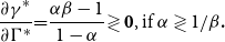 \begin{equation*} \frac {\partial \gamma ^{\ast }}{\partial \Gamma ^{\ast }}\mathbf {=}\frac {\alpha \beta -1}{1-\alpha }\mathbf {\gtrless 0}\text {, if }\alpha \gtrless 1/\beta \mathbf {.} \end{equation*}
To examine the dynamic property of this model, we linearize the dynamic system (41) and (42) around the steady state as follows:
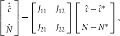 \begin{equation} \left [ \begin{array}{c} \overset{\centerdot }{\hat{c}} \\[5pt] \overset{\centerdot }{N}\end{array}\right ] =\left [ \begin{array}{c@{\quad}c} J_{11} & J_{12} \\[5pt] J_{21} & J_{22}\end{array}\right ] \left [ \begin{array}{c} \hat{c}-\hat{c}^{\ast } \\[5pt] N-N^{\ast }\end{array}\right ], \end{equation}
where $J_{11}=\left ( 1+\Theta \hat{c}^{\ast }\right ) (1-\tau _{\Pi })\frac{1-\alpha }{\beta -1}\frac{1-\theta }{\theta }\theta ^{\frac{2}{1-\theta }}\frac{\hat{c}^{\ast }L_{\hat{c}}}{N^{\ast }}\lt 0$
,
$J_{11}=\left ( 1+\Theta \hat{c}^{\ast }\right ) (1-\tau _{\Pi })\frac{1-\alpha }{\beta -1}\frac{1-\theta }{\theta }\theta ^{\frac{2}{1-\theta }}\frac{\hat{c}^{\ast }L_{\hat{c}}}{N^{\ast }}\lt 0$
, $J_{12}=\left ( 1+\Theta \hat{c}^{\ast }\right ) (1-\tau _{\Pi })\frac{1-\alpha }{\beta -1}\frac{1-\theta }{\theta }\theta ^{\frac{2}{1-\theta }}\frac{-\hat{c}^{\ast }L_{\hat{c}}}{\left ( N^{\ast }\right ) ^{2}}$ $\lt 0$
,
$\lt 0$
, $J_{21}=\frac{1}{\beta }\left ( -\frac{1}{\theta ^{2}}\theta ^{\frac{2}{1-\theta }}\frac{L^{\ast }}{N^{\ast }}+\Phi \frac{L_{\hat{c}}}{L^{\ast }}\right ) N^{\ast }\lt 0$
,
$J_{21}=\frac{1}{\beta }\left ( -\frac{1}{\theta ^{2}}\theta ^{\frac{2}{1-\theta }}\frac{L^{\ast }}{N^{\ast }}+\Phi \frac{L_{\hat{c}}}{L^{\ast }}\right ) N^{\ast }\lt 0$
, $J_{22}=-\frac{1}{\beta }\Phi \lt 0$
,
$J_{22}=-\frac{1}{\beta }\Phi \lt 0$
, $L_{\hat{c}}=\frac{-\Theta }{\left ( 1+\Theta \hat{c}^{\ast }\right ) ^{2}}$
, and
$L_{\hat{c}}=\frac{-\Theta }{\left ( 1+\Theta \hat{c}^{\ast }\right ) ^{2}}$
, and $\Phi \equiv \left ( \frac{1-\tau _{\Pi }}{\beta -1}+1\right ) \phi +\frac{\beta \lambda ^{\ast }\sigma (\lambda ^{\ast })}{1+\tilde{\lambda }}$
. It follows from (A5) that the trace and the determinant of the Jacobian matrix are as follows:
$\Phi \equiv \left ( \frac{1-\tau _{\Pi }}{\beta -1}+1\right ) \phi +\frac{\beta \lambda ^{\ast }\sigma (\lambda ^{\ast })}{1+\tilde{\lambda }}$
. It follows from (A5) that the trace and the determinant of the Jacobian matrix are as follows:
 \begin{equation*} \text{Tr}=\left ( 1+\Theta \hat {c}^{\ast }\right ) (1-\tau _{\Pi })\frac {1-\alpha }{\beta -1}\frac {1-\theta }{\theta }\theta ^{\frac {2}{1-\theta }}\frac {\hat {c}^{\ast }L_{\hat {c}}}{N^{\ast }}-\frac {1}{\beta }\Phi \lt 0, \end{equation*}
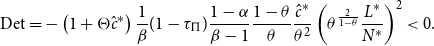 \begin{equation*} \text{Det}=-\left ( 1+\Theta \hat {c}^{\ast }\right ) \frac {1}{\beta }(1-\tau _{\Pi })\frac {1-\alpha }{\beta -1}\frac {1-\theta }{\theta }\frac {\hat {c}^{\ast }}{\theta ^{2}}\left ( \theta ^{\frac {2}{1-\theta }}\frac {L^{\ast }}{N^{\ast }}\right ) ^{2}\lt 0. \end{equation*}
Because there is one jump variable $\hat{c}$
and one state variable
$\hat{c}$
and one state variable $N$
in the model, the Routh−Hurwitz stability criterion indicates that the dynamic system is locally determinate.
$N$
in the model, the Routh−Hurwitz stability criterion indicates that the dynamic system is locally determinate.
APPENDIX B: COMPARATIVE STATICS
B.1. Effects of the dividend tax
From (27), we have $\lambda _{\tau _{D}}^{\ast }=\frac{\partial \lambda ^{\ast }}{\partial \tau _{D}}=\frac{1}{\Sigma }\frac{i^{E}}{1-\tau _{V}}\gt 0$
, where
$\lambda _{\tau _{D}}^{\ast }=\frac{\partial \lambda ^{\ast }}{\partial \tau _{D}}=\frac{1}{\Sigma }\frac{i^{E}}{1-\tau _{V}}\gt 0$
, where $\Sigma =\frac{1-\tau _{\Pi }}{1-\tau _{B}}\!\left [ 2\sigma ^{\prime }(\lambda ^{\ast })+\lambda ^{\ast }\sigma ^{\prime \prime }(\lambda ^{\ast })\right ]\! (1+\lambda ^{\ast })\gt 0$
. Accordingly, taking the partial derivative of (28) with respect to
$\Sigma =\frac{1-\tau _{\Pi }}{1-\tau _{B}}\!\left [ 2\sigma ^{\prime }(\lambda ^{\ast })+\lambda ^{\ast }\sigma ^{\prime \prime }(\lambda ^{\ast })\right ]\! (1+\lambda ^{\ast })\gt 0$
. Accordingly, taking the partial derivative of (28) with respect to $\tau _{D}$
yields
$\tau _{D}$
yields $\Gamma _{\tau _{D}}^{\ast }=\frac{1}{1+\lambda ^{\ast }}\frac{i^{E}}{1-\tau _{V}}\gt 0$
. Equipped with
$\Gamma _{\tau _{D}}^{\ast }=\frac{1}{1+\lambda ^{\ast }}\frac{i^{E}}{1-\tau _{V}}\gt 0$
. Equipped with $(\Psi ^{In})^{\ast }=(1-\tau _{\Pi })\alpha \frac{1-\theta }{\theta }\left ( \frac{x}{z}\right ) ^{\ast }$
,
$(\Psi ^{In})^{\ast }=(1-\tau _{\Pi })\alpha \frac{1-\theta }{\theta }\left ( \frac{x}{z}\right ) ^{\ast }$
, $(\Psi ^{En})^{\ast }=\frac{1-\tau _{\Pi }}{\beta }\left [ \frac{1-\theta }{\theta }\left ( \frac{x}{z}\right ) ^{\ast }-\phi \right ]$
, and (A1), we take the differentials of
$(\Psi ^{En})^{\ast }=\frac{1-\tau _{\Pi }}{\beta }\left [ \frac{1-\theta }{\theta }\left ( \frac{x}{z}\right ) ^{\ast }-\phi \right ]$
, and (A1), we take the differentials of $(\Psi ^{In})^{\ast }$
and
$(\Psi ^{In})^{\ast }$
and $(\Psi ^{En})^{\ast }$
with respect to
$(\Psi ^{En})^{\ast }$
with respect to $\tau _{D}$
, respectively, yielding
$\tau _{D}$
, respectively, yielding $\Psi _{\tau _{D}}^{In}=\frac{\partial (\Psi ^{In})^{\ast }}{\partial \tau _{D}}=\frac{\alpha (\beta -1)}{1-\alpha }\Gamma _{\tau _{D}}^{\ast }\gt 0$
and
$\Psi _{\tau _{D}}^{In}=\frac{\partial (\Psi ^{In})^{\ast }}{\partial \tau _{D}}=\frac{\alpha (\beta -1)}{1-\alpha }\Gamma _{\tau _{D}}^{\ast }\gt 0$
and $\Psi _{\tau _{D}}^{En}=\frac{\partial (\Psi ^{En})^{\ast }}{\partial \tau _{D}}=\frac{\beta -1}{\beta (1-\alpha )}\Gamma _{\tau _{D}}^{\ast }\gt 0$
. Moreover, differentiating (43) and (44) with respect to
$\Psi _{\tau _{D}}^{En}=\frac{\partial (\Psi ^{En})^{\ast }}{\partial \tau _{D}}=\frac{\beta -1}{\beta (1-\alpha )}\Gamma _{\tau _{D}}^{\ast }\gt 0$
. Moreover, differentiating (43) and (44) with respect to $\tau _{D}$
, respectively, we obtain:
$\tau _{D}$
, respectively, we obtain:
 \begin{equation*} \frac {\partial \gamma ^{\ast }}{\partial \tau _{D}}=\frac {\alpha \beta -1}{1-\alpha }\Gamma _{\tau _{D}}^{\ast }\gtrless 0, \, \text{if} \, \alpha \beta -1\gtrless 0, \end{equation*}
 \begin{equation*} \frac {\partial \pi ^{\ast }}{\partial \tau _{D}}=\left [ 1-\frac {\alpha (\beta -1)}{1-\alpha }\right ] \Gamma _{\tau _{D}}^{\ast }=\frac {1-\alpha \beta }{1-\alpha }\Gamma _{\tau _{D}}^{\ast }\lessgtr 0,\text { if }\alpha \beta -1\gtrless 0. \end{equation*}
Differentiating (A2), (A3), and (39) with respect to $\tau _{D}$
further yields:
$\tau _{D}$
further yields:
 \begin{equation*} \frac {\partial \hat {c}^{\ast }}{\partial \tau _{D}}=\frac {\theta ^{2}}{\left ( \frac {x}{z}\right ) ^{\ast }}\left [ \frac {\Phi \Gamma _{\tau _{D}}^{\ast }}{\Gamma ^{\ast }-(1-\tau _{B})\overline {i}+\rho +\frac {1-\tau _{\Pi }}{\beta -1}\phi }-\beta \frac {\sigma (\lambda ^{\ast })+\lambda ^{\ast }\sigma ^{\prime }(\lambda ^{\ast })\left ( 1+\lambda ^{\ast }\right ) }{\left ( 1+\lambda ^{\ast }\right ) ^{2}}\lambda _{\tau _{D}}^{\ast }\right ] \gtrless 0, \end{equation*}
 \begin{equation*} \frac {\partial N^{\ast }}{\partial \tau _{D}}=-N^{\ast }\Theta L^{\ast }\cdot \frac {\partial \hat {c}^{\ast }}{\partial \tau _{D}}-\frac {N^{\ast }}{(\Psi ^{In})^{\ast }}\frac {\alpha (\beta -1)}{1-\alpha }\Gamma _{\tau _{D}}^{\ast }\lessgtr 0. \end{equation*}
 \begin{equation*} \frac {\partial L^{\ast }}{\partial \tau _{D}}=-\Theta \!\left ( L^{\ast }\right ) ^{2}\cdot \frac {\partial \hat {c}^{\ast }}{\partial \tau _{D}}\lessgtr 0, \end{equation*}
B.2. Effects of the corporate tax
According to (27), we have $\lambda _{\tau _{\Pi }}^{\ast }=\frac{\partial \lambda ^{\ast }}{\partial \tau _{\Pi }}=\frac{1}{\Sigma }\left [ \overline{i}+\frac{\sigma (\lambda ^{\ast })+\lambda ^{\ast }\sigma ^{\prime }(\lambda ^{\ast })\left ( 1+\lambda ^{\ast }\right ) }{1-\tau _{B}}\right ] \gt 0$
. Taking the partial derivative of (28) with respect to
$\lambda _{\tau _{\Pi }}^{\ast }=\frac{\partial \lambda ^{\ast }}{\partial \tau _{\Pi }}=\frac{1}{\Sigma }\left [ \overline{i}+\frac{\sigma (\lambda ^{\ast })+\lambda ^{\ast }\sigma ^{\prime }(\lambda ^{\ast })\left ( 1+\lambda ^{\ast }\right ) }{1-\tau _{B}}\right ] \gt 0$
. Taking the partial derivative of (28) with respect to $\tau _{\Pi }$
yields
$\tau _{\Pi }$
yields $\Gamma _{\tau _{\Pi }}^{\ast }=\frac{-\lambda ^{\ast }}{1+\lambda ^{\ast }}\left [ \overline{i}+\frac{\sigma (\lambda ^{\ast })}{1-\tau _{B}}\right ] \lt 0$
. By taking the differentials of
$\Gamma _{\tau _{\Pi }}^{\ast }=\frac{-\lambda ^{\ast }}{1+\lambda ^{\ast }}\left [ \overline{i}+\frac{\sigma (\lambda ^{\ast })}{1-\tau _{B}}\right ] \lt 0$
. By taking the differentials of $(\Psi ^{In})^{\ast }$
and
$(\Psi ^{In})^{\ast }$
and $(\Psi ^{En})^{\ast }$
with respect to
$(\Psi ^{En})^{\ast }$
with respect to $\tau _{\Pi }$
, we can obtain
$\tau _{\Pi }$
, we can obtain $\Psi _{\tau _{\Pi }}^{In}=\frac{\partial (\Psi ^{In})^{\ast }}{\partial \tau _{\Pi }}=\frac{\alpha (\beta -1)}{1-\alpha }\left ( \Gamma _{\tau _{\Pi }}^{\ast }-\frac{\phi }{\beta -1}\right ) \lt 0$
and
$\Psi _{\tau _{\Pi }}^{In}=\frac{\partial (\Psi ^{In})^{\ast }}{\partial \tau _{\Pi }}=\frac{\alpha (\beta -1)}{1-\alpha }\left ( \Gamma _{\tau _{\Pi }}^{\ast }-\frac{\phi }{\beta -1}\right ) \lt 0$
and $\Psi _{\tau _{\Pi }}^{En}=\frac{\partial (\Psi ^{En})^{\ast }}{\partial \tau _{\Pi }}=\frac{\beta -1}{\beta \left ( 1-\alpha \right ) }\left ( \Gamma _{\tau _{\Pi }}^{\ast }-\frac{\alpha \phi }{\beta -1}\right ) \lt 0$
, respectively. Moreover, differentiating partially (43) and (44) with respect to
$\Psi _{\tau _{\Pi }}^{En}=\frac{\partial (\Psi ^{En})^{\ast }}{\partial \tau _{\Pi }}=\frac{\beta -1}{\beta \left ( 1-\alpha \right ) }\left ( \Gamma _{\tau _{\Pi }}^{\ast }-\frac{\alpha \phi }{\beta -1}\right ) \lt 0$
, respectively. Moreover, differentiating partially (43) and (44) with respect to $\tau _{\Pi }$
yields:
$\tau _{\Pi }$
yields:
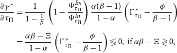 \begin{align*} \frac {\partial \gamma ^{\ast }}{\partial \tau _{\Pi }} &= \frac {1}{1-\frac {1}{\beta }}\left ( 1-\frac {\Psi _{\tau _{\Pi }}^{En}}{\Psi _{\tau _{\Pi }}^{In}}\right ) \frac {\alpha (\beta -1)}{1-\alpha }\left ( \Gamma _{\tau _{\Pi }}^{\ast }-\frac {\phi }{\beta -1}\right ) \\[5pt] & = \frac {\alpha \beta -\Xi }{1-\alpha }\left ( \Gamma _{\tau _{\Pi }}^{\ast }-\frac {\phi }{\beta -1}\right ) \lessgtr 0, \, \text {if }\alpha \beta -\Xi \gtrless 0, \end{align*}
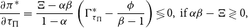 \begin{equation*} \frac {\partial \pi ^{\ast }}{\partial \tau _{\Pi }}=\frac {\Xi -\alpha \beta }{1-\alpha }\left ( \Gamma _{\tau _{\Pi }}^{\ast }-\frac {\phi }{\beta -1}\right ) \lessgtr 0, \, \text{if} \, \alpha \beta -\Xi \gtrless 0, \end{equation*}
where $\Xi =\frac{\Gamma _{\tau _{\Pi }}^{\ast }-\frac{\alpha \phi }{\beta -1}}{\Gamma _{\tau _{\Pi }}^{\ast }-\frac{\phi }{\beta -1}}\in (0,1)$
. In addition, differentiating partially (A2), (A3), and (39) with respect to
$\Xi =\frac{\Gamma _{\tau _{\Pi }}^{\ast }-\frac{\alpha \phi }{\beta -1}}{\Gamma _{\tau _{\Pi }}^{\ast }-\frac{\phi }{\beta -1}}\in (0,1)$
. In addition, differentiating partially (A2), (A3), and (39) with respect to $\tau _{\Pi }$
, respectively, yields:
$\tau _{\Pi }$
, respectively, yields:
 \begin{equation*} \frac {\partial \hat {c}^{\ast }}{\partial \tau _{\Pi }}=\frac {\theta ^{2}}{\left ( \frac {x}{z}\right ) ^{\ast }}\left [ \frac {\Phi\!\left ( \Gamma _{\tau _{\Pi }}^{\ast }-\frac {\phi }{\beta -1}\right ) }{\Gamma ^{\ast }\text {-}(1-\tau _{B})\overline {i}\text {+}\rho \text {+}\frac {1-\tau _{\Pi }}{\beta -1}\phi }\text {+}\frac {\phi }{\beta \text {-}1}-\beta \frac {\sigma (\lambda ^{\ast })\text {+}\lambda ^{\ast }\sigma ^{\prime }(\lambda ^{\ast })\left ( 1\text {+}\lambda ^{\ast }\right ) }{\left ( 1\text {+}\lambda ^{\ast }\right ) ^{2}}\lambda _{\tau _{\Pi }}^{\ast }\right ] \text {+}\frac {1\text {-}\hat {c}^{\ast }\text {-}\varphi \text {-}\theta ^{2}}{1-\tau _{\Pi }}\gtrless 0, \end{equation*}
 \begin{equation*} \frac {\partial N^{\ast }}{\partial \tau _{\Pi }}=-\frac {N^{\ast }}{1-\tau _{\Pi }}-N^{\ast }\Theta L^{\ast }\cdot \frac {\partial \hat {c}^{\ast }}{\partial \tau _{\Pi }}-\frac {N^{\ast }}{(\Psi ^{In})^{\ast }}\frac {\alpha (\beta -1)}{1-\alpha }\left ( \Gamma _{\tau _{\Pi }}^{\ast }-\frac {\phi }{\beta -1}\right ) \lessgtr 0, \end{equation*}
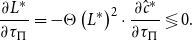 \begin{equation*} \frac {\partial L^{\ast }}{\partial \tau _{\Pi }}=-\Theta \left ( L^{\ast }\right ) ^{2}\cdot \frac {\partial \hat {c}^{\ast }}{\partial \tau _{\Pi }}\lessgtr 0. \end{equation*}
B.3. Effects of the bond income tax
From (27), we have $\tilde{\lambda }_{\tau _{B}}=\frac{\partial \lambda ^{\ast }}{\partial \tau _{B}}=\frac{-1}{\Sigma \left ( 1-\tau _{V}\right ) }\left \{ \overline{i}+\frac{1-\tilde{\tau }}{1-\tau _{B}}\left [ \sigma (\lambda ^{\ast })+\lambda ^{\ast }\sigma ^{\prime }(\lambda ^{\ast })\left ( 1+\lambda ^{\ast }\right ) \right ] \right \} \lt 0$
and, accordingly, taking the partial derivative of (28) with respect to
$\tilde{\lambda }_{\tau _{B}}=\frac{\partial \lambda ^{\ast }}{\partial \tau _{B}}=\frac{-1}{\Sigma \left ( 1-\tau _{V}\right ) }\left \{ \overline{i}+\frac{1-\tilde{\tau }}{1-\tau _{B}}\left [ \sigma (\lambda ^{\ast })+\lambda ^{\ast }\sigma ^{\prime }(\lambda ^{\ast })\left ( 1+\lambda ^{\ast }\right ) \right ] \right \} \lt 0$
and, accordingly, taking the partial derivative of (28) with respect to $\tau _{B}$
yields
$\tau _{B}$
yields $\Gamma _{\tau _{B}}^{\ast }=\frac{1}{1+\lambda ^{\ast }}[\frac{(1-\tau _{\Pi })\lambda ^{\ast }\sigma (\lambda ^{\ast })}{\left ( 1-\tau _{B}\right ) ^{2}}-\frac{\overline{i}}{1-\tau _{V}}]\gtreqless 0$
. Given that
$\Gamma _{\tau _{B}}^{\ast }=\frac{1}{1+\lambda ^{\ast }}[\frac{(1-\tau _{\Pi })\lambda ^{\ast }\sigma (\lambda ^{\ast })}{\left ( 1-\tau _{B}\right ) ^{2}}-\frac{\overline{i}}{1-\tau _{V}}]\gtreqless 0$
. Given that $(\Psi ^{In})^{\ast }=(1-\tau _{\Pi })\alpha \frac{1-\theta }{\theta }\left ( \frac{x}{z}\right ) ^{\ast }$
and
$(\Psi ^{In})^{\ast }=(1-\tau _{\Pi })\alpha \frac{1-\theta }{\theta }\left ( \frac{x}{z}\right ) ^{\ast }$
and $(\Psi ^{En})^{\ast }=\frac{1-\tau _{\Pi }}{\beta }(\frac{1-\theta }{\theta }\left ( \frac{x}{z}\right ) ^{\ast }-\phi )$
(together with (A1)), taking the differentials of
$(\Psi ^{En})^{\ast }=\frac{1-\tau _{\Pi }}{\beta }(\frac{1-\theta }{\theta }\left ( \frac{x}{z}\right ) ^{\ast }-\phi )$
(together with (A1)), taking the differentials of $(\Psi ^{In})^{\ast }$
and
$(\Psi ^{In})^{\ast }$
and $(\Psi ^{En})^{\ast }$
with respect to
$(\Psi ^{En})^{\ast }$
with respect to $\tau _{B}$
yields
$\tau _{B}$
yields $\Psi _{\tau _{B}}^{In}=\frac{\partial (\Psi ^{In})^{\ast }}{\partial \tau _{B}}=\frac{\alpha (\beta -1)}{1-\alpha }\left ( \Gamma _{\tau _{B}}^{\ast }+\overline{i}\right ) \gtrless 0$
and
$\Psi _{\tau _{B}}^{In}=\frac{\partial (\Psi ^{In})^{\ast }}{\partial \tau _{B}}=\frac{\alpha (\beta -1)}{1-\alpha }\left ( \Gamma _{\tau _{B}}^{\ast }+\overline{i}\right ) \gtrless 0$
and $\Psi _{\tau _{B}}^{En}=\frac{\partial (\Psi ^{En})^{\ast }}{\partial \tau _{B}}=\frac{\beta -1}{\beta \left ( 1-\alpha \right ) }\left ( \Gamma _{\tau _{B}}^{\ast }+\overline{i}\right ) \gtrless 0$
, respectively. Moreover, differentiating partially (43) and (44) with respect to
$\Psi _{\tau _{B}}^{En}=\frac{\partial (\Psi ^{En})^{\ast }}{\partial \tau _{B}}=\frac{\beta -1}{\beta \left ( 1-\alpha \right ) }\left ( \Gamma _{\tau _{B}}^{\ast }+\overline{i}\right ) \gtrless 0$
, respectively. Moreover, differentiating partially (43) and (44) with respect to $\tau _{B}$
, respectively, yields:
$\tau _{B}$
, respectively, yields:
 \begin{equation*} \frac {\partial \gamma ^{\ast }}{\partial \tau _{B}}=\frac {\alpha \beta -1}{1-\alpha }\left ( \Gamma _{\tau _{B}}^{\ast }+\overline {i}\right ) \gtrless 0,\ \text {if }(\alpha \beta -1)\left ( \Gamma _{\tau _{B}}^{\ast }+\overline {i}\right ) \gtrless 0, \end{equation*}
 \begin{equation*} \frac {\partial \pi ^{\ast }}{\partial \tau _{B}}=\frac {1-\alpha \beta }{1-\alpha }\Gamma _{\tau _{B}}^{\ast }-\frac {\alpha (\beta -1)}{1-\alpha }\overline {i}\lessgtr 0. \end{equation*}
Sequentially, differentiating partially (A2), (A3), and (39) with respect to $\tau _{B}$
yields:
$\tau _{B}$
yields:
 \begin{equation*} \frac {\partial \hat {c}^{\ast }}{\partial \tau _{B}}=\frac {\theta ^{2}}{\left ( \frac {x}{z}\right ) ^{\ast }}\left [ \frac {\Phi \left ( \Gamma _{\tau _{B}}^{\ast }+\overline {i}\right ) }{\Gamma ^{\ast }-(1-\tau _{B})\overline {i}+\rho +\frac {1-\tau _{\Pi }}{\beta -1}\phi }-\beta \frac {\sigma (\lambda ^{\ast })+\lambda ^{\ast }\sigma ^{\prime }(\lambda ^{\ast })\left ( 1+\lambda ^{\ast }\right ) }{\left ( 1+\lambda ^{\ast }\right ) ^{2}}\lambda _{\tau _{B}}^{\ast }\right ] \gtrless 0, \end{equation*}
 \begin{equation*} \frac {\partial N^{\ast }}{\partial \tau _{B}}=\frac {N^{\ast }(1-L^{\ast })\overline {i}}{(1+\tau _{c})+(1-\tau _{B})\overline {i}}-N^{\ast }\Theta L^{\ast }\cdot \frac {\partial \hat {c}^{\ast }}{\partial \tau _{B}}-\frac {N^{\ast }}{(\Psi ^{In})^{\ast }}\frac {\alpha (\beta -1)}{1-\alpha }\left ( \Gamma _{\tau _{B}}^{\ast }+\overline {i}\right ) \lessgtr 0, \end{equation*}
 \begin{equation*} \frac {\partial L^{\ast }}{\partial \tau _{B}}=\frac {L^{\ast }(1-L^{\ast })\overline {i}}{(1+\tau _{c})+(1-\tau _{B})\overline {i}}-\Theta \left ( L^{\ast }\right ) ^{2}\cdot \frac {\partial \hat {c}^{\ast }}{\partial \tau _{B}}\lessgtr 0. \end{equation*}
B.4. Effects of the nominal interest rate
From (27), we have $\lambda _{\overline{i}}^{\ast }=\frac{\partial \lambda ^{\ast }}{\partial \overline{i}}=\frac{1}{\Sigma }\frac{1-\tau _{B}}{1-\tau _{V}}\tilde{\tau }\gt 0$
. Taking the partial derivative of (28) with respect to
$\lambda _{\overline{i}}^{\ast }=\frac{\partial \lambda ^{\ast }}{\partial \overline{i}}=\frac{1}{\Sigma }\frac{1-\tau _{B}}{1-\tau _{V}}\tilde{\tau }\gt 0$
. Taking the partial derivative of (28) with respect to $\overline{i}$
yields
$\overline{i}$
yields $\Gamma _{\overline{i}}^{\ast }=\frac{1}{1+\lambda ^{\ast }}\left [ \left ( 1-\tau _{\Pi }\right ) \lambda ^{\ast }+\frac{1-\tau _{B}}{1-\tau _{V}}\right ] \gt 0$
. Given
$\Gamma _{\overline{i}}^{\ast }=\frac{1}{1+\lambda ^{\ast }}\left [ \left ( 1-\tau _{\Pi }\right ) \lambda ^{\ast }+\frac{1-\tau _{B}}{1-\tau _{V}}\right ] \gt 0$
. Given $(\Psi ^{In})^{\ast }$
,
$(\Psi ^{In})^{\ast }$
, $(\Psi ^{En})^{\ast }$
, and (A1), we take the differentials of
$(\Psi ^{En})^{\ast }$
, and (A1), we take the differentials of $(\Psi ^{In})^{\ast }$
and
$(\Psi ^{In})^{\ast }$
and $(\Psi ^{En})^{\ast }$
with respect to
$(\Psi ^{En})^{\ast }$
with respect to $\overline{i}$
and obtain
$\overline{i}$
and obtain $\Psi _{\overline{i}}^{In}=\frac{\partial (\Psi ^{In})^{\ast }}{\partial \overline{i}}=\frac{\alpha (\beta -1)}{1-\alpha }\left [ \Gamma _{\overline{i}}^{\ast }-(1-\tau _{B})\right ] \gtrless 0$
and
$\Psi _{\overline{i}}^{In}=\frac{\partial (\Psi ^{In})^{\ast }}{\partial \overline{i}}=\frac{\alpha (\beta -1)}{1-\alpha }\left [ \Gamma _{\overline{i}}^{\ast }-(1-\tau _{B})\right ] \gtrless 0$
and $\Psi _{\overline{i}}^{En}=\frac{\partial (\Psi ^{En})^{\ast }}{\partial \overline{i}}=\frac{\beta -1}{\beta (1-\alpha )}\left [ \Gamma _{\overline{i}}^{\ast }-(1-\tau _{B})\right ] \gtrless 0$
, respectively. Furthermore, differentiating partially (43) and (44) with respect to
$\Psi _{\overline{i}}^{En}=\frac{\partial (\Psi ^{En})^{\ast }}{\partial \overline{i}}=\frac{\beta -1}{\beta (1-\alpha )}\left [ \Gamma _{\overline{i}}^{\ast }-(1-\tau _{B})\right ] \gtrless 0$
, respectively. Furthermore, differentiating partially (43) and (44) with respect to $\overline{i}$
, respectively, yields:
$\overline{i}$
, respectively, yields:
 \begin{equation*} \frac {\partial \gamma ^{\ast }}{\partial \overline {i}}=\frac {\alpha \beta -1}{1-\alpha }\left [ \Gamma _{\overline {i}}^{\ast }-(1-\tau _{B})\right ] \gtrless 0, \, \text{if} \, \left ( \alpha \beta -1\right ) \left [ \Gamma _{\overline {i}}^{\ast }-(1-\tau _{B})\right ] \gtrless 0, \end{equation*}
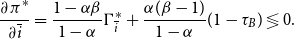 \begin{equation*} \frac {\partial \pi ^{\ast }}{\partial \overline {i}}=\frac {1-\alpha \beta }{1-\alpha }\Gamma _{\overline {i}}^{\ast }+\frac {\alpha (\beta -1)}{1-\alpha }(1-\tau _{B})\lessgtr 0. \end{equation*}
Then, differentiating partially (A2), (A3), and (39) with respect to $\overline{i}$
, respectively, yields:
$\overline{i}$
, respectively, yields:
 \begin{equation*} \frac {\partial \hat {c}^{\ast }}{\partial \overline {i}}=\frac {\theta ^{2}}{\left ( \frac {x}{z}\right ) ^{\ast }}\left \{ \frac {\Phi \left [ \Gamma _{\overline {i}}^{\ast }-(1-\tau _{B})\right ] }{\Gamma ^{\ast }-(1-\tau _{B})\overline {i}+\rho +\frac {1-\tau _{\Pi }}{\beta -1}\phi }-\beta \frac {\sigma (\lambda ^{\ast })+\lambda ^{\ast }\sigma ^{\prime }(\lambda ^{\ast })\left ( 1+\lambda ^{\ast }\right ) }{\left ( 1+\lambda ^{\ast }\right ) ^{2}}\lambda _{\overline {i}}^{\ast }\right \} \gtrless 0, \end{equation*}
 \begin{equation*} \frac {\partial N^{\ast }}{\partial \overline {i}}=-N^{\ast }\hat {c}^{\ast }L^{\ast }\frac {\delta }{1-\theta }\frac {1-\tau _{B}}{1-\tau _{L}}-N^{\ast }\Theta L^{\ast }\cdot \frac {\partial \hat {c}^{\ast }}{\partial \overline {i}}-\frac {N^{\ast }}{(\Psi ^{In})^{\ast }}\frac {\alpha (\beta -1)}{1-\alpha }\left [ \Gamma _{\overline {i}}^{\ast }-(1-\tau _{B})\right ] \lessgtr 0, \end{equation*}
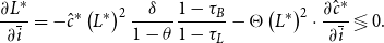 \begin{equation*} \frac {\partial L^{\ast }}{\partial \overline {i}}=-\hat {c}^{\ast }\left ( L^{\ast }\right ) ^{2}\frac {\delta }{1-\theta }\frac {1-\tau _{B}}{1-\tau _{L}}-\Theta \left ( L^{\ast }\right ) ^{2}\cdot \frac {\partial \hat {c}^{\ast }}{\partial \overline {i}}\lessgtr 0. \end{equation*}


