


1. Introduction
The distributional impact of government spending on agents’ disposable income has been an important research topic in the macroeconomics literature. Recently, Anderson et al. (Reference Anderson, D’Orey, Duvendack and Esposito2017) carry out a meta-regression analysis to synthesize empirical findings from $84$
econometric studies with more than
$84$
econometric studies with more than $900$
estimates that have quantified the aggregate effects of various categories of public expenditures on several measures of posttax income inequality. On the whole, these authors find a moderate and statistically significant inverse relationship between public spending and income inequality. Moreover, based on the panel data from multiple samples of OECD countries over the 1981–2005 period, Doerrenberg and Peichl (Reference Doerrenberg and Peichl2014) report that a 1% increase in the GDP share of total government purchases generates decreases in (i) the net-income Gini coefficient by 0.23%–0.38% per fixed effects panel regressions; or (ii) an inequality measure estimated from the University of Texas Inequality Project (UTIP) data by 0.328%–0.333% per the instrumental variable approach. Guzi and Kahanec (Reference Guzi and Kahanec2018) also empirically investigated this subject with a panel dataset from
$900$
estimates that have quantified the aggregate effects of various categories of public expenditures on several measures of posttax income inequality. On the whole, these authors find a moderate and statistically significant inverse relationship between public spending and income inequality. Moreover, based on the panel data from multiple samples of OECD countries over the 1981–2005 period, Doerrenberg and Peichl (Reference Doerrenberg and Peichl2014) report that a 1% increase in the GDP share of total government purchases generates decreases in (i) the net-income Gini coefficient by 0.23%–0.38% per fixed effects panel regressions; or (ii) an inequality measure estimated from the University of Texas Inequality Project (UTIP) data by 0.328%–0.333% per the instrumental variable approach. Guzi and Kahanec (Reference Guzi and Kahanec2018) also empirically investigated this subject with a panel dataset from $30$
advanced European economies for the time period of 2004–2015. Under two different sets of control variables, their fixed effects estimation yields that the resulting calculated elasticities of after-tax Gini with respect to government size (in absolute terms) are
$30$
advanced European economies for the time period of 2004–2015. Under two different sets of control variables, their fixed effects estimation yields that the resulting calculated elasticities of after-tax Gini with respect to government size (in absolute terms) are $0.22$
and
$0.22$
and $0.26$
, respectively—these results turn out to be quantitatively consistent with Doerrenberg and Peichl’s (Reference Doerrenberg and Peichl2014, Table 1) earlier estimates.Footnote 1 In sum, these previous studies, together with numerous references therein, illustrate that there exists a discernible negative correlation between total government expenditure and after-tax income inequality, and that the estimated calculated elasticities range over the interval
$0.26$
, respectively—these results turn out to be quantitatively consistent with Doerrenberg and Peichl’s (Reference Doerrenberg and Peichl2014, Table 1) earlier estimates.Footnote 1 In sum, these previous studies, together with numerous references therein, illustrate that there exists a discernible negative correlation between total government expenditure and after-tax income inequality, and that the estimated calculated elasticities range over the interval $[0.22$
,
$[0.22$
, $0.38]$
.
$0.38]$
.
The objective of our paper is to develop a tractable dynamic general equilibrium model that is able to yield qualitatively as well as quantitatively realistic net income inequality effects of government spending in accordance with the aforementioned empirical evidence. Therefore, this is a piece of positive macroeconomic research which abstracts from deriving the optimal fiscal policy and/or examining the related normative/welfare issues. Taking a modified version of García-Peñalosa and Turnovsky’s (Reference García-Peñalosa and Turnovsky2011) Ramsey model as the point of departure, we incorporate monopolistic competition and free entry/exit of intermediate goods-producing firms into an economy with infinitely lived heterogeneous households that differ only in their initial capital endowments.Footnote 2 Under the postulated homogenous and isoelastic preference formulation, we are able to analytically obtain the transitional dynamics and steady-state dispersions of wealth/capital and disposable income in terms of the economy-wide aggregate variables [Caselli and Ventura (Reference Caselli and Ventura2000)]. The production side of our macroeconomy consists of an intermediate good segment, whereby monopolistically competitive firms operate under preset constant overhead costs and a Cobb–Douglas production function using capital and labor as inputs. A final output is produced from the set of available differentiated intermediate goods in a perfectly competitive environment. For the baseline setting, public expenditures are assumed to be useless which do not contribute to firms’ production or agents’ utility functions. The government balances the budget at each instant of time by levying only lump-sum taxes on households to finance its purchases of final goods and services. These simplifications enable us to isolate how changes in the public-spending share affect the long-run distribution of after-tax income as well as facilitate direct comparisons with the above-cited empirical studies in a focused and transparent manner. To provide a useful reference point for the subsequent quantitative results, numerical experiments are also conducted for our model economy under perfect competition, as in García-Peñalosa and Turnovsky (Reference García-Peñalosa and Turnovsky2011).
We first analytically derive that at the model’s unique steady state, the standard deviation of agents’ disposable income is proportional to that of their relative capital stock by a positive scaling parameter as a function of the public-spending share. We then show that in response to an increase in the GDP proportion of government purchases, the long-run dispersion of after-tax income may rise or fall depending on the directions as well as the strengths of two distinct effects. On the one hand, since a higher government size raises the steady-state aggregate capital stock, the macroeconomy undertakes more capital investment along the unique convergent equilibrium path toward the new long-run distribution of wealth measured in terms of relative capital stock. During the transition instants of time, capital-rich households will choose to work less and slow down their wealth accumulation rate, whereas capital-poor individuals will supply more hours worked and accumulate their wealth at a faster rate. As a result, the new stationary equilibrium distribution of relative capital stock becomes less unequal than the initial counterpart—this is dubbed as the wealth/capital inequality effect that is always negative. On the other hand, we find that the sign for the above-mentioned scaling parameter is theoretically ambiguous, determined by whether the economy-wide labor supply (adjusted by nongovernmental expenditure share) rises or falls upon the occurrence of a larger public sector—this is dubbed as the adjusted-labor effect. When these two effects are of the same sign (opposite signs), the overall steady-state distributional consequence of an increase in government spending on households’ disposal income will be a lower (higher or lower) degree of inequality.
Given the inconclusive nature of the preceding theoretical results, a quantitative assessment is undertaken within a calibrated version of our macroeconomy. In addition to assigning benchmark values to model parameters, different levels of market competitiveness are considered to numerically gauge the importance of imperfectly competitive product markets. We first find that the adjusted-labor effect is negative for each parametric configuration under consideration. This, together with the unambiguously negative wealth/capital inequality effect, implies that a higher public-spending share will decrease the steady-state standard deviation of disposable income in our baseline setting. However, the resulting calculated elasticity of after-tax Gini with respect to public expenditures under perfect competition ( $=0.0515$
) is significantly lower than the estimated range of 0.22–0.38 reported by Doerrenberg and Peichl (Reference Doerrenberg and Peichl2014) and Guzi and Kahanec (Reference Guzi and Kahanec2018). When the degree of monopoly market power rises, the economy’s speed of convergence toward the new stationary state will be relatively slower, which in turn enhances the declining dispersion of agents’ relative capital distribution along the transition path. As a result, the wealth/capital inequality effect becomes stronger, but the calculated elasticities remain too low to be empirically realistic. In the context of our benchmark Ramsey model, it is shown that monopolistic competition alone does not lead to a quantitative match with the actual data on the long-run distributional consequences of public expenditures.
$=0.0515$
) is significantly lower than the estimated range of 0.22–0.38 reported by Doerrenberg and Peichl (Reference Doerrenberg and Peichl2014) and Guzi and Kahanec (Reference Guzi and Kahanec2018). When the degree of monopoly market power rises, the economy’s speed of convergence toward the new stationary state will be relatively slower, which in turn enhances the declining dispersion of agents’ relative capital distribution along the transition path. As a result, the wealth/capital inequality effect becomes stronger, but the calculated elasticities remain too low to be empirically realistic. In the context of our benchmark Ramsey model, it is shown that monopolistic competition alone does not lead to a quantitative match with the actual data on the long-run distributional consequences of public expenditures.
In light of these numerical findings from the baseline framework, we examine an otherwise identical monopolistically competitive Ramsey model with useful government purchases of goods and services, either being productive or utility-generating. While keeping other parameter values unchanged, incorporating productive public spending à la Barro (Reference Barro1990) results in a higher percentage increase of the stationary aggregate capital stock as the public expenditure share increases. This outcome will slow down the capital accumulation rate toward the new steady state, which in turn decreases the posttax income dispersion because of a stronger wealth/capital inequality effect. Under the logarithmically separable preference formulation in consumption and leisure, the perfectly competitive version of our model with a mild level of productive government-spending externalities delivers a calculated elasticity ( $=0.222$
) that is marginally above the lower bound of the estimated interval
$=0.222$
) that is marginally above the lower bound of the estimated interval $[0.22$
,
$[0.22$
, $0.38]$
. When either the monopolistic market power or each agent’s intertemporal elasticity of consumption substitution rises, the resulting elasticities of after-tax Gini with respect to government purchases will increase to 0.2301–0.3373, which are a much closer fit with the empirical evidence. We also find that under nonseparable utility-generating public expenditures à la García-Peñalosa and Turnovsky (Reference García-Peñalosa and Turnovsky2011), the long-run distribution of agents’ labor hours will become less unequal in response to a higher government size, regardless of whether private consumption and public goods are Edgeworth substitutes or complements. This in turn leads to a weaker wealth/capital inequality effect because of the negative correlation between the dispersion of labor supply and that of relative capital stock during the transition. In this environment, the calculated elasticities will be lower than those in the benchmark model with wasteful government purchases; hence, they are not empirically plausible either.
$0.38]$
. When either the monopolistic market power or each agent’s intertemporal elasticity of consumption substitution rises, the resulting elasticities of after-tax Gini with respect to government purchases will increase to 0.2301–0.3373, which are a much closer fit with the empirical evidence. We also find that under nonseparable utility-generating public expenditures à la García-Peñalosa and Turnovsky (Reference García-Peñalosa and Turnovsky2011), the long-run distribution of agents’ labor hours will become less unequal in response to a higher government size, regardless of whether private consumption and public goods are Edgeworth substitutes or complements. This in turn leads to a weaker wealth/capital inequality effect because of the negative correlation between the dispersion of labor supply and that of relative capital stock during the transition. In this environment, the calculated elasticities will be lower than those in the benchmark model with wasteful government purchases; hence, they are not empirically plausible either.
Overall, this paper shows that our calibrated monopolistically competitive Ramsey model with (i) a mild level of productive public-expenditure externalities and (ii) a sufficiently high intertemporal elasticity of substitution (IES) in consumption is able to generate qualitatively as well as quantitatively realistic net-income-inequality effects of government spending vis-à-vis recent econometric studies, for example, Doerrenberg and Peichl (Reference Doerrenberg and Peichl2014) and Guzi and Kahanec (Reference Guzi and Kahanec2018). In terms of relevant references, Chatterjee and Turnovsky (Reference Chatterjee and Turnovsky2012) examine an endogenously growing macroeconomy with public capital entering the representative firm’s production technology. Under lump-sum taxation (as in our analysis), these authors find that an increase in government spending on infrastructure will raise the long-run wealth/capital and income inequalities. These results, which are qualitatively inconsistent with the data and opposite to ours, imply that how productive public expenditures are considered matters. Subsequently, Klenert et al. (Reference Klenert, Mattauch, Edenhofer and Lessmann2018) studied an overlapping generations model with agent heterogeneities in saving propensities, income sources, and time preference rates and numerically show that the long-run wealth/capital and income inequality impacts of higher public investment can be positive, neutral, or negative, depending on whether government spending is financed through taxation on the households’ labor income, consumption expenditures, or capital income.
The remainder of this paper is organized as follows. Section 2 describes our baseline Ramsey macroeconomy, discusses its equilibrium conditions and distributional dynamics, and then analytically derive the Gini coefficient associated with the long-run distribution of agents’ disposable income. Section 3 theoretically as well as quantitatively examines the income-inequality effects of government spending within the benchmark model. Section 4 studies an otherwise identical monopolistically competitive economy with productive or utility-generating public expenditures of final goods and services. Section 5 concludes.
2. The economy
Our analysis begins with incorporating monopolistic competition and free entry/exit of intermediate goods-producing firms into a simplified version of García-Peñalosa and Turnovsky’s (Reference García-Peñalosa and Turnovsky2011) Ramsey model with heterogeneous households in continuous time. Agents live forever and derive utilities from consumption and leisure under a homogeneous and isoelastic preference formulation, and they only differ in terms of their initial capital endowments. On the production side of our macroeconomy, there is an intermediate-good segment in which monopolistically competitive firms operate with fixed setup costs and a constant returns-to-scale Cobb–Douglas production technology using capital and labor as inputs. The equilibrium size and measure of these intermediate-input producers are endogenously pinned down by the zero-profit condition. A final output (GDP) is produced from the set of available differentiated intermediate goods in a perfectly competitive environment. The government balances the budget at each instant of time by levying lump-sum taxes on households to finance its purchases of final goods and services. For the sake of analytical simplicity, public expenditures are postulated to be useless which do not contribute to firms’ production or agents’ utility functions within our baseline setting. In addition, population growth, non-unitary elasticity of substitution between capital and labor in production, as well as other forms of taxation (e.g., capital, labor, or consumption) are not considered. These simplifications streamline our exposition that will enable us to examine the distributional effects of government spending under imperfect competition in a focused and transparent manner.
2.1. Firms
The production side of our model economy consists of two segments. As in Devereux et al. (Reference Devereux, Head and Lapham1996, Reference Devereux, Head and Lapham2000), a single homogeneous final good $Y_{t}$
is produced from a continuum of intermediate inputs
$Y_{t}$
is produced from a continuum of intermediate inputs $x_{jt}$
with the following production technology:
$x_{jt}$
with the following production technology:
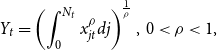 \begin{equation} Y_{t}=\left ( \int _{0}^{N_{t}}x_{jt}^{\rho }dj\right ) ^{\frac{1}{\rho }}, \, 0\lt \rho \lt 1, \end{equation}
where $N_{t}$
denotes the measure of (as well as the degree of variety for) intermediate goods utilized at time
$N_{t}$
denotes the measure of (as well as the degree of variety for) intermediate goods utilized at time $t$
, and
$t$
, and $\rho$
governs the elasticity of substitution between distinct intermediate inputs.Footnote 3 The final-good segment is postulated to be perfectly competitive, and we denote
$\rho$
governs the elasticity of substitution between distinct intermediate inputs.Footnote 3 The final-good segment is postulated to be perfectly competitive, and we denote $p_{jt}$
as the price of the
$p_{jt}$
as the price of the $j$
’th intermediate good relative to the final output. The final-goods-producing firms’ profit maximization condition yields that
$j$
’th intermediate good relative to the final output. The final-goods-producing firms’ profit maximization condition yields that
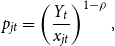 \begin{equation} p_{jt}=\left ( \frac{Y_{t}}{x_{jt}}\right ) ^{1-\rho }, \end{equation}
where the price elasticity of demand for $x_{jt}$
is
$x_{jt}$
is $\frac{1}{1-\rho }$
, and the resulting markup ratio of price over marginal cost, given by
$\frac{1}{1-\rho }$
, and the resulting markup ratio of price over marginal cost, given by $\frac{1}{\rho }$
, characterizes the degree of market power for intermediate-good producers. In the limiting case of
$\frac{1}{\rho }$
, characterizes the degree of market power for intermediate-good producers. In the limiting case of $\rho =1$
, all intermediate inputs are perfect substitutes for the production of
$\rho =1$
, all intermediate inputs are perfect substitutes for the production of $Y_{t}$
; therefore, the demand curve (2) will become perfectly elastic or horizontal.
$Y_{t}$
; therefore, the demand curve (2) will become perfectly elastic or horizontal.
Each intermediate good is produced by a monopolist with the Cobb–Douglas production specification in its own factor inputs:
 \begin{equation} x_{jt}=Ak_{jt}^{a}h_{jt}^{b}-Z, {\quad} A,a,b,Z\gt 0 \quad \textrm{and} \quad a+b=1, \end{equation}
where $A$
captures the technological state,
$A$
captures the technological state, $k_{jt}$
and
$k_{jt}$
and $h_{jt}$
are capital and labor services employed by the
$h_{jt}$
are capital and labor services employed by the $j$
’th intermediate-input firm, respectively, and
$j$
’th intermediate-input firm, respectively, and $Z$
represents a constant amount of intermediate goods that must be expended as fixed setup costs before any production is undertaken. Such overhead costs will affect noncompetitive firms’ potential incentive to enter the market, which in turn help determine the equilibrium size/quantity (as shown in (5)) and measure/variety (see (7)) of these producers. Since
$Z$
represents a constant amount of intermediate goods that must be expended as fixed setup costs before any production is undertaken. Such overhead costs will affect noncompetitive firms’ potential incentive to enter the market, which in turn help determine the equilibrium size/quantity (as shown in (5)) and measure/variety (see (7)) of these producers. Since $a+b=1$
, the incidence of
$a+b=1$
, the incidence of $Z\gt 0$
implies that the intermediate-goods technology (3) exhibits increasing returns-to-scale. We also note that when
$Z\gt 0$
implies that the intermediate-goods technology (3) exhibits increasing returns-to-scale. We also note that when $\rho =1$
and
$\rho =1$
and $Z=0$
, the economy’s production structure will collapse to one with only perfectly competitive final-goods-producing firms, as studied by García-Peñalosa and Turnovsky (Reference García-Peñalosa and Turnovsky2011).
$Z=0$
, the economy’s production structure will collapse to one with only perfectly competitive final-goods-producing firms, as studied by García-Peñalosa and Turnovsky (Reference García-Peñalosa and Turnovsky2011).
Using equations (2) and (3), together with the assumption that factor markets are perfectly competitive, it is straightforward to show that the first-order conditions for the $j$
’th intermediate-input producer’s profit maximization problem are as follows:
$j$
’th intermediate-input producer’s profit maximization problem are as follows:
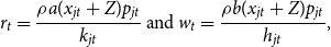 \begin{equation} r_{t}=\frac{\rho a(x_{jt}+Z)p_{jt}}{k_{jt}} \, \textrm{and} \, w_{t}=\frac{\rho b(x_{jt}+Z)p_{jt}}{h_{jt}}, \end{equation}
where $r_{t}$
is the capital rental rate and
$r_{t}$
is the capital rental rate and $w_{t}$
is the real wage rate. Under free entry and exit for intermediate goods-producing firms, their profit will be equal to zero at each instant of time. This zero-profit condition together with (4) yield the constant equilibrium quantity of intermediate input
$w_{t}$
is the real wage rate. Under free entry and exit for intermediate goods-producing firms, their profit will be equal to zero at each instant of time. This zero-profit condition together with (4) yield the constant equilibrium quantity of intermediate input $j$
:
$j$
:
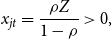 \begin{equation} x_{jt}=\frac{\rho Z}{1-\rho }\gt 0, \end{equation}
which also represents the $j$
’th intermediate-good producer’s size that turns out to be independent of any endogenous variable. In what follows, our analysis is restricted to the model’s symmetric equilibrium in which
$j$
’th intermediate-good producer’s size that turns out to be independent of any endogenous variable. In what follows, our analysis is restricted to the model’s symmetric equilibrium in which
 \begin{equation} p_{jt}=p_{t}\textrm{, }x_{jt}=x_{t},\textrm{ }k_{jt}=\frac{K_{t}}{N_{t}},\textrm{ }h_{jt}=\frac{H_{t}}{N_{t}},\textrm{ for all }j\in \lbrack 0,\textrm{ }N_{t}], \end{equation}
where $K_{t}\left ( =\int _{0}^{N_{t}}k_{jt}dj\right )$
and
$K_{t}\left ( =\int _{0}^{N_{t}}k_{jt}dj\right )$
and $H_{t}\left ( =\int _{0}^{N_{t}}h_{jt}dj\right )$
denote the total capital stock and labor hours demanded or employed by intermediate-input firms, respectively. Using equations (3), (5), and (6), it can be shown that the equilibrium measure/variety of intermediate-good producers is
$H_{t}\left ( =\int _{0}^{N_{t}}h_{jt}dj\right )$
denote the total capital stock and labor hours demanded or employed by intermediate-input firms, respectively. Using equations (3), (5), and (6), it can be shown that the equilibrium measure/variety of intermediate-good producers is
 \begin{equation} N_{t}=\left [ \frac{A\left ( 1-\rho \right ) }{Z}\right ] K_{t}^{a}H_{t}^{b}\gt 0. \end{equation}
Next, after substituting (6)–(7) into (1) and (3), we find that the economy’s reduced-form production function is given by:
 \begin{equation} Y_{t}=N_{t}^{\frac{1}{\rho }}x_{t}=\rho \left ( \frac{1-\rho }{Z}\right ) ^{\frac{1-\rho }{\rho }}\left ( AK_{t}^{a}H_{t}^{b}\right ) ^{\frac{1}{\rho }}, \end{equation}
where $\frac{a}{\rho }\lt 1$
to rule out the possibility of sustained endogenous growth and
$\frac{a}{\rho }\lt 1$
to rule out the possibility of sustained endogenous growth and $N_{t}^{\frac{1}{\rho }}$
represents a measure of economy-wide productivity. Since the monopolistic-markup parameter
$N_{t}^{\frac{1}{\rho }}$
represents a measure of economy-wide productivity. Since the monopolistic-markup parameter $\rho$
lies over the interval
$\rho$
lies over the interval $(0$
,
$(0$
, $1)$
, the aggregate technology (8) will exhibit increasing returns to an expansion in product variety
$1)$
, the aggregate technology (8) will exhibit increasing returns to an expansion in product variety $N_{t}$
[Bénassy (Reference Bénassy1996)], which can be interpreted as endogenously enhancing the economy’s total factor productivity. In addition, the level of aggregate returns-to-scale in production with respect to total capital and labor inputs is equal to
$N_{t}$
[Bénassy (Reference Bénassy1996)], which can be interpreted as endogenously enhancing the economy’s total factor productivity. In addition, the level of aggregate returns-to-scale in production with respect to total capital and labor inputs is equal to $\frac{1}{\rho }\gt 1$
.
$\frac{1}{\rho }\gt 1$
.
Finally, plugging (6) and (8) into (2) shows that the symmetric equilibrium price of each intermediate good is
 \begin{equation} p_{t}=N_{t}^{\frac{1-\rho }{\rho }}, \end{equation}
where $N_{t}$
is given by (7). We can then combine equations (4)–(9) to derive that the symmetric equilibrium factor prices are
$N_{t}$
is given by (7). We can then combine equations (4)–(9) to derive that the symmetric equilibrium factor prices are
 \begin{equation} r_{t}=a\frac{Y_{t}}{K_{t}}, \end{equation}
 \begin{equation} w_{t}=b\frac{Y_{t}}{H_{t}}, \end{equation}
hence, the capital and labor shares of national income are equal to $a$
and
$a$
and $b$
, respectively.
$b$
, respectively.
2.2. Households
The economy is inhabited by a large number of infinitely lived households whose population size is normalized to one for all $t$
. These heterogeneous agents are indexed by
$t$
. These heterogeneous agents are indexed by $i$
that is uniformly distributed over the interval
$i$
that is uniformly distributed over the interval $[0$
,
$[0$
, $1]$
. As in Turnovsky and García-Peñalosa (Reference Turnovsky and García-Peñalosa2008), individual
$1]$
. As in Turnovsky and García-Peñalosa (Reference Turnovsky and García-Peñalosa2008), individual $i$
is endowed with one unit of labor hour at each instant of time and an initial level of capital stock
$i$
is endowed with one unit of labor hour at each instant of time and an initial level of capital stock $K_{i0}$
and maximizes a discounted stream of utilities over its lifetime:
$K_{i0}$
and maximizes a discounted stream of utilities over its lifetime:
 \begin{equation} \int _{0}^{\infty }\underbrace{\frac{1}{\gamma }\left ( C_{it}\ell _{it}^{\eta }\right ) ^{\gamma }}_{\equiv \textrm{ }U_{it}}e^{-\beta t}dt,\, \,-\infty \lt \gamma \lt 1, \,\, \eta,\, \, \beta \gt 0,\, \, \textrm{and }\,\gamma \eta \lt 1, \end{equation}
where $C_{it}$
is consumption,
$C_{it}$
is consumption, $\ell _{it}$
is leisure,
$\ell _{it}$
is leisure, $\beta$
is the subjective rate of time preference,
$\beta$
is the subjective rate of time preference, $\frac{1}{1-\gamma }$
determines the IES in “effective consumption”
$\frac{1}{1-\gamma }$
determines the IES in “effective consumption” $C_{it}\ell _{it}^{\eta }$
, and
$C_{it}\ell _{it}^{\eta }$
, and $U_{it}$
is a homogenous utility function of degree
$U_{it}$
is a homogenous utility function of degree $\gamma \left ( 1+\eta \right )$
. Notice that when
$\gamma \left ( 1+\eta \right )$
. Notice that when $\gamma =0$
, each household’s preference formulation becomes separable and logarithmic in both consumption and leisure, that is,
$\gamma =0$
, each household’s preference formulation becomes separable and logarithmic in both consumption and leisure, that is, $U_{it}=\log C_{it}+\eta \log \ell _{it}$
.
$U_{it}=\log C_{it}+\eta \log \ell _{it}$
.
The budget constraint faced by individual $i$
is given by:
$i$
is given by:
 \begin{equation} \dot{K}_{it}=r_{t}K_{it}+w_{t}H_{it}+\pi _{it}-C_{it}-T_{it}-\delta K_{it},\, \,K_{i0}\gt 0\, \ \textrm{given,} \end{equation}
where $H_{it}\left ( =1-\ell _{it}\right )$
denotes hours worked,
$H_{it}\left ( =1-\ell _{it}\right )$
denotes hours worked, $\pi _{it}$
represents the profits as lump-sum dividends from agent
$\pi _{it}$
represents the profits as lump-sum dividends from agent $i$
’s ownership of intermediate-good firms,
$i$
’s ownership of intermediate-good firms, $T_{it}$
denotes lump-sum taxes collected by the government, and
$T_{it}$
denotes lump-sum taxes collected by the government, and $\delta$ $\in (0,1)$
is the capital depreciation rate. The first-order conditions for this particular household’s dynamic optimization problem are
$\in (0,1)$
is the capital depreciation rate. The first-order conditions for this particular household’s dynamic optimization problem are
 \begin{equation} C_{it}^{\gamma -1}\ell _{it}^{\eta \gamma }=\lambda _{it}, \end{equation}
 \begin{equation} \eta \frac{C_{it}}{\ell _{it}}=w_{t}, \end{equation}
 \begin{equation} \frac{\dot{\lambda }_{it}}{\lambda _{it}}=\beta +\delta -r_{t}, \end{equation}
 \begin{equation} \underset{t\rightarrow \infty }{\lim }\lambda _{it}K_{it}e^{-\beta t}=0, \end{equation}
where $\lambda _{it}$
denotes the costate variable that characterizes the shadow (utility) value of physical capital. In addition, (15) equates the slope of individual
$\lambda _{it}$
denotes the costate variable that characterizes the shadow (utility) value of physical capital. In addition, (15) equates the slope of individual $i$
’s indifference curve to the real wage, (16) is the consumption Euler equation, and (17) is the transversality condition. After substituting (15) into (13), the capital accumulation equation for household
$i$
’s indifference curve to the real wage, (16) is the consumption Euler equation, and (17) is the transversality condition. After substituting (15) into (13), the capital accumulation equation for household $i$
can be written as:
$i$
can be written as:
 \begin{equation} \frac{\dot{K}_{it}}{K_{it}}=r_{t}-\delta +\left ( 1-\frac{1+\eta }{\eta }\ell _{it}\right ) \frac{w_{t}}{K_{it}}+\frac{\pi _{it}-T_{it}}{K_{it}}. \end{equation}
2.3. Government
The government spends its total (lump-sum) tax revenues $T_{t}$
on goods and services produced by final-output producers and maintains a balanced budget at each instant of time. Hence, its instantaneous budget constraint is given by:
$T_{t}$
on goods and services produced by final-output producers and maintains a balanced budget at each instant of time. Hence, its instantaneous budget constraint is given by:
 \begin{equation} G_{t}=T_{t}=\int _{0}^{1}T_{it}di, \end{equation}
where $G_{t}$
is public expenditures that are postulated to be a constant fraction of the economy’s aggregate output:
$G_{t}$
is public expenditures that are postulated to be a constant fraction of the economy’s aggregate output:
 \begin{equation} G_{t}=gY_{t}, \ 0\lt g\lt 1, \end{equation}
where $Y_{t}$
is given by (8). Finally, combining the aggregated version of (13), together with
$Y_{t}$
is given by (8). Finally, combining the aggregated version of (13), together with $\pi _{it}=0$
for all
$\pi _{it}=0$
for all $i$
and
$i$
and $t$
, and (19) yields the following economy-wide resource constraint:
$t$
, and (19) yields the following economy-wide resource constraint:
 \begin{equation} C_{t}+I_{t}+G_{t}=Y_{t}, \end{equation}
where $C_{t}\left ( =\int _{0}^{1}C_{it}di\right )$
denotes total consumption spending and
$C_{t}\left ( =\int _{0}^{1}C_{it}di\right )$
denotes total consumption spending and $I_{t}\left ( =\int _{0}^{1}\left [ \dot{K}_{it}+\delta K_{it}\right ] di\right )$
represents total gross investment.
$I_{t}\left ( =\int _{0}^{1}\left [ \dot{K}_{it}+\delta K_{it}\right ] di\right )$
represents total gross investment.
2.4. Macroeconomic Equilibrium
This subsection derives the economy’s equilibrium allocations expressed in terms of aggregate variables. We first take the time derivative on individual $i$
’s marginal utility of consumption, given by (14), to obtain
$i$
’s marginal utility of consumption, given by (14), to obtain
 \begin{equation} (\gamma -1)\frac{\dot{C}_{it}}{C_{it}}+\eta \gamma \frac{\dot{\ell }_{it}}{\ell _{it}}=\frac{\dot{\lambda }_{it}}{\lambda _{it}}, \end{equation}
which is equal to $\beta +\delta -r_{t}$
that is independent of
$\beta +\delta -r_{t}$
that is independent of $i$
[see equation (16)]. This in turn implies that all agents choose the same growth rate for the shadow value of capital, regardless of how their capital endowments are initially distributed. We then take the time derivative on household
$i$
[see equation (16)]. This in turn implies that all agents choose the same growth rate for the shadow value of capital, regardless of how their capital endowments are initially distributed. We then take the time derivative on household $i$
’s labor supply decision (15) and follow Turnovsky and García-Peñalosa (Reference Turnovsky and García-Peñalosa2008, Appendix A.1) to find that
$i$
’s labor supply decision (15) and follow Turnovsky and García-Peñalosa (Reference Turnovsky and García-Peñalosa2008, Appendix A.1) to find that
 \begin{equation} \frac{\dot{C}_{it}}{C_{it}}=\frac{\dot{C}_{t}}{C_{t}}{ \ \textrm{and} \ }\frac{\dot{\ell }_{it}}{\ell _{it}}=\frac{\dot{\ell }_{t}}{\ell _{t}} \ \textrm{for all}\ i \ \textrm{and} \ t\textrm{,} \end{equation}
where $\ell _{t}\left ( =\int _{0}^{1}\ell _{it}di\right )$
denotes total leisure time. Equation (23) states that individual and aggregate quantities of consumption and leisure will grow at their respective common rates. In accordance with Caselli and Ventura (Reference Caselli and Ventura2000), the postulated homogenous and isoelastic preference formulation (12) results in macroeconomic equilibrium allocations that are independent of the wealth/capital distribution within our model and identical to those in the corresponding representative agent setting which begins with an exogenously given
$\ell _{t}\left ( =\int _{0}^{1}\ell _{it}di\right )$
denotes total leisure time. Equation (23) states that individual and aggregate quantities of consumption and leisure will grow at their respective common rates. In accordance with Caselli and Ventura (Reference Caselli and Ventura2000), the postulated homogenous and isoelastic preference formulation (12) results in macroeconomic equilibrium allocations that are independent of the wealth/capital distribution within our model and identical to those in the corresponding representative agent setting which begins with an exogenously given $K_{0}\left ( =\int _{0}^{1}K_{i0}di\right )$
. Moreover, the equalities of aggregate demand by intermediate goods-producing firms versus aggregate supply by heterogeneous households in the capital and labor markets are given by:
$K_{0}\left ( =\int _{0}^{1}K_{i0}di\right )$
. Moreover, the equalities of aggregate demand by intermediate goods-producing firms versus aggregate supply by heterogeneous households in the capital and labor markets are given by:
 \begin{equation} \int _{0}^{N_{t}}k_{jt}dj=K_{t}=\int _{0}^{1}K_{it}di, \end{equation}
 \begin{equation} \int _{0}^{N_{t}}h_{jt}dj=H_{t}=\int _{0}^{1}H_{it}di. \end{equation}
Finally, taking aggregation over each household’s first-order conditions as in (15) and (18), together with $\pi _{t}\left ( =\int _{0}^{1}\pi _{it}di\right ) =0$
and equations (8), (10)–(11), (19)–(20), and (24)–(25), yields that the economy-wide level of capital will accumulate over time according to
$\pi _{t}\left ( =\int _{0}^{1}\pi _{it}di\right ) =0$
and equations (8), (10)–(11), (19)–(20), and (24)–(25), yields that the economy-wide level of capital will accumulate over time according to
 \begin{equation} \frac{\dot{K}_{t}}{K_{t}}=\rho A^{^{\frac{1}{\rho }}}\left ( \frac{1-\rho }{Z}\right ) ^{\frac{1-\rho }{\rho }}\left [ (1-g)H_{t}-\frac{b}{\eta }(1-H_{t})\right ] K_{t}^{\frac{a}{\rho }-1}H_{t}^{\frac{b}{\rho }-1}-\delta,\, \,K_{0}\gt 0 \ \textrm{ given.} \end{equation}
In addition, we use the aggregated version of condition (15), as well as equations (8), (11), and (22)–(25), to obtain the evolution of aggregate labor hours:
 \begin{equation} \frac{\dot{H}_{t}}{H_{t}}=\frac{\beta +\delta +\left [ \frac{a(1-\gamma )}{\rho }\right ] \frac{\dot{K}_{t}}{K_{t}}-\rho aA^{^{\frac{1}{\rho }}}\left ( \frac{1-\rho }{Z}\right ) ^{\frac{1-\rho }{\rho }}K_{t}^{\frac{a}{\rho }-1}H_{t}^{\frac{b}{\rho }}}{(1-\gamma )\left ( 1-\frac{b}{\rho }\right ) +[1-\gamma (1+\eta )]\left ( \frac{H_{t}}{1-H_{t}}\right ) }. \end{equation}
It follows that our baseline model’s equilibrium conditions can be characterized by an autonomous pair of differential equations à la (26) and (27), indicating that the dynamics of aggregate capital $K_{t}$
and aggregate labor
$K_{t}$
and aggregate labor $H_{t}$
are not affected by the initial wealth/capital distribution.
$H_{t}$
are not affected by the initial wealth/capital distribution.
2.5. Steady State
By setting $\dot{K}_{t}=\dot{H}_{t}=0$
in (26) and (27), it is straightforward to show that our imperfectly competitive macroeconomy possesses a unique interior steady state given by:
$\dot{K}_{t}=\dot{H}_{t}=0$
in (26) and (27), it is straightforward to show that our imperfectly competitive macroeconomy possesses a unique interior steady state given by:
 \begin{equation} \tilde{H}=\frac{b(\beta +\delta )}{(\beta +\delta )[b+(1-g)\eta ]-a\eta \delta }, \end{equation}
 \begin{equation} \tilde{K}=\left [ A\left ( \frac{1-\rho }{Z}\right ) ^{1-\rho }\left ( \frac{\rho a}{\beta +\delta }\right ) ^{\rho }\tilde{H}^{b}\right ] ^{\frac{1}{\rho -a}}. \end{equation}
The remaining endogenous variables at the economy’s stationary state can then be derived accordingly. Furthermore, under the empirically realistic assumption that labor income accounts for a smaller percentage of GDP than households’ aggregate consumption spending, the steady-state version of (26) leads to the following inequality:Footnote 4
 \begin{equation} \tilde{H}\lt \frac{1}{1+\eta }, \end{equation}
which places an upper bound on the stationary economy-wide level of hours worked. From equation (28), it can then be shown that the effect on $\tilde{H}$
of a permanent change in the output share of government purchases
$\tilde{H}$
of a permanent change in the output share of government purchases $g$
is
$g$
is
 \begin{equation} \frac{\partial \tilde{H}}{\partial g}=\frac{b\eta (\beta +\delta )^{2}}{\left \{ (\beta +\delta )[b+(1-g)\eta ]-a\eta \delta \right \} ^{2}}\gt 0. \end{equation}
As it is well known in the modern macroeconomics literature, a higher national income share of public spending (financed by additional lump-sum taxes on households) will raise the steady-state labor supply because of a negative wealth effect. However, this response is independent of the monopolistic-markup parameter $\rho$
because it does not enter the expression for
$\rho$
because it does not enter the expression for $\tilde{H}$
. Since
$\tilde{H}$
. Since $\frac{\partial \tilde{K}}{\partial \tilde{H}}\gt 0$
per equation (29), we also note that the stationary level of aggregate capital stock becomes higher upon an increase in
$\frac{\partial \tilde{K}}{\partial \tilde{H}}\gt 0$
per equation (29), we also note that the stationary level of aggregate capital stock becomes higher upon an increase in $g$
.
$g$
.
2.6. Equilibrium Dynamics
In the neighborhood of the unique interior stationary state given by (28) and (29), our model’s equilibrium conditions can be approximated by the linearized dynamical system:
 \begin{equation} \left [ \begin{array}{l} \dot{K}_{t} \\ \dot{H}_{t}\end{array}\right ] =\underbrace{\left [ \begin{array}{ll} a_{11} & a_{12} \\ a_{21} & a_{22}\end{array}\right ] }_{\mathbf{J}}\left [ \begin{array}{l} K_{t}-\tilde{K} \\ H_{t}-\tilde{H}\end{array}\right ],{ \ }K_{0}\gt 0 \ \textrm{ given,} \end{equation}
where $\mathbf{J}$
is the Jacobian matrix of partial derivatives, and the analytical expressions for its elements are shown in Appendix. As in Turnovsky and García-Peñalosa (Reference Turnovsky and García-Peñalosa2008) and García-Peñalosa and Turnovsky (Reference García-Peñalosa and Turnovsky2011), our subsequent analysis will be restricted to environments in which the model’s steady state is a locally determinate saddle point. Since the first-order dynamical system (26)–(27) possesses one predetermined variable
$\mathbf{J}$
is the Jacobian matrix of partial derivatives, and the analytical expressions for its elements are shown in Appendix. As in Turnovsky and García-Peñalosa (Reference Turnovsky and García-Peñalosa2008) and García-Peñalosa and Turnovsky (Reference García-Peñalosa and Turnovsky2011), our subsequent analysis will be restricted to environments in which the model’s steady state is a locally determinate saddle point. Since the first-order dynamical system (26)–(27) possesses one predetermined variable $K_{t}$
, the economy displays saddle-path stability and equilibrium uniqueness if and only if the two real eigenvalues of
$K_{t}$
, the economy displays saddle-path stability and equilibrium uniqueness if and only if the two real eigenvalues of $\mathbf{J}$
are of opposite signs with
$\mathbf{J}$
are of opposite signs with $Det(\mathbf{J)}=a_{11}a_{22}-a_{12}a_{21}\lt 0$
. After some tedious but manageable algebra, we find that the requisite necessary and sufficient condition for local determinacy, expressed in terms of a lower bound on the monopolistic-markup parameter, is
$Det(\mathbf{J)}=a_{11}a_{22}-a_{12}a_{21}\lt 0$
. After some tedious but manageable algebra, we find that the requisite necessary and sufficient condition for local determinacy, expressed in terms of a lower bound on the monopolistic-markup parameter, is
 \begin{equation} \rho \gt \underbrace{\frac{b\eta (1-\gamma )[(b-g)\delta +(1-g)\beta ]}{\eta (1-\gamma )[(b-g)\delta +(1-g)\beta ]+b(\beta +\delta )[1-\gamma (1+\eta )]}}_{\equiv \textrm{ }\rho _{\min }}, \end{equation}
under which the Jacobian’s two eigenvalues are characterized by $\mu \lt 0\lt \upsilon$
. It follows that the stable branch of the economy’s saddle path can be written as:
$\mu \lt 0\lt \upsilon$
. It follows that the stable branch of the economy’s saddle path can be written as:
 \begin{equation} K_{t}=\tilde{K}+(K_{0}-\tilde{K})e^{\mu t}, \end{equation}
and
 \begin{equation} H_{t}=\tilde{H}+\frac{\mu -a_{11}}{a_{12}}(K_{t}-\tilde{K}), \end{equation}
where $a_{11}\lt 0$
and
$a_{11}\lt 0$
and $a_{12}\gt 0$
per the proof in Appendix.
$a_{12}\gt 0$
per the proof in Appendix.
Intuitively, an increase in capital stock will reduce its growth rate because of diminishing marginal product of capital inputs associated with the aggregate production function (8); thus, $\left. \frac{\partial \dot{K}_{t}}{\partial K_{t}}\right \vert _{\dot{K}_{t}\textrm{ }=\textrm{ }0}=a_{11}$
is negative. In addition, a higher level of hours worked raises the rate of return to investment [see equation (10)], which in turn will increase the accumulation rate of capital; thus,
$\left. \frac{\partial \dot{K}_{t}}{\partial K_{t}}\right \vert _{\dot{K}_{t}\textrm{ }=\textrm{ }0}=a_{11}$
is negative. In addition, a higher level of hours worked raises the rate of return to investment [see equation (10)], which in turn will increase the accumulation rate of capital; thus, $\left. \frac{\partial \dot{K}_{t}}{\partial H_{t}}\right \vert _{\dot{K}_{t}\textrm{ }=\textrm{ }0}=a_{12}$
is positive. On the other hand, the speed of convergence for the economy’s equilibrium path toward the stationary state is determined by the modulus of
$\left. \frac{\partial \dot{K}_{t}}{\partial H_{t}}\right \vert _{\dot{K}_{t}\textrm{ }=\textrm{ }0}=a_{12}$
is positive. On the other hand, the speed of convergence for the economy’s equilibrium path toward the stationary state is determined by the modulus of $\mu$
, whose magnitude depends on model parameters in a rather complicated manner. It follows that the sign for the stable arm of the saddle point, given by
$\mu$
, whose magnitude depends on model parameters in a rather complicated manner. It follows that the sign for the stable arm of the saddle point, given by $\frac{\mu -a_{11}}{a_{12}}$
, is theoretically ambiguous. For all the empirically plausible parameterizations that are considered in Sections 3.2 and 4, our model’s stable locus (35) is negatively sloped; therefore, labor hours are monotonically decreasing with respect to capital stock along the transition path.Footnote 5 Given this relationship holds at each instant of time, we obtain that the initial labor supply relative to its steady-state level is governed by:
$\frac{\mu -a_{11}}{a_{12}}$
, is theoretically ambiguous. For all the empirically plausible parameterizations that are considered in Sections 3.2 and 4, our model’s stable locus (35) is negatively sloped; therefore, labor hours are monotonically decreasing with respect to capital stock along the transition path.Footnote 5 Given this relationship holds at each instant of time, we obtain that the initial labor supply relative to its steady-state level is governed by:
 \begin{equation} H_{0}-\tilde{H}=\underbrace{\frac{\mu -a_{11}}{a_{12}}}_{\textrm{Negative}}(K_{0}-\tilde{K}). \end{equation}
Since $K_{0}$
is exogenously given and
$K_{0}$
is exogenously given and $\{ \mu$
,
$\{ \mu$
, $a_{11}$
,
$a_{11}$
, $a_{12}$
,
$a_{12}$
, $\tilde{K}$
,
$\tilde{K}$
, $\tilde{H}\}$
are functions of model parameters, equation (36) can be used to (endogenously) determine the unique value of
$\tilde{H}\}$
are functions of model parameters, equation (36) can be used to (endogenously) determine the unique value of $H_{0}$
that will place the economy on the convergent equilibrium trajectory.
$H_{0}$
that will place the economy on the convergent equilibrium trajectory.
2.7. After-Tax Income Inequality
This subsection analytically derives the economy’s income inequality measured by the Gini coefficient based on the steady-state distribution of households’ relative after-tax income. To this end, we follow García-Peñalosa and Turnovsky (Reference García-Peñalosa and Turnovsky2011) and postulate that the dynamic paths of individual and aggregate taxes-to-capital ratios are identical, that is, $\frac{T_{it}}{K_{it}}=\frac{T_{t}}{K_{t}}$
for all
$\frac{T_{it}}{K_{it}}=\frac{T_{t}}{K_{t}}$
for all $i$
and
$i$
and $t$
.Footnote 6 Using the definition of
$t$
.Footnote 6 Using the definition of $k_{it}\equiv \frac{K_{it}}{K_{t}}$
to denote agent
$k_{it}\equiv \frac{K_{it}}{K_{t}}$
to denote agent $i$
’s relative capital stock and
$i$
’s relative capital stock and $\pi _{it}=0$
because of free entry/exit of intermediate goods-producing firms, we combine equations (18) and (26) to derive that
$\pi _{it}=0$
because of free entry/exit of intermediate goods-producing firms, we combine equations (18) and (26) to derive that
 \begin{equation} \dot{k}_{it}=\frac{w_{t}}{K_{t}}\left \{ \left [ \frac{(1+\eta )H_{it}-1}{\eta }\right ] -\left [ \frac{(1+\eta )H_{t}-1}{\eta }\right ] k_{it}\right \} \textrm{, }\ k_{i0}\gt 0\ \textrm{ given.} \end{equation}
It follows that at the model’s stationary state with $\dot{k}_{it}=0$
,
$\dot{k}_{it}=0$
,
 \begin{equation} \tilde{H}_{i}-\tilde{H}=\left ( \tilde{H}-\frac{1}{1+\eta }\right ) \left ( \widetilde{k}_{i}-\underbrace{\widetilde{k}}_{=\textrm{ }1}\right ) \end{equation}
holds for each household, where $\tilde{H}-\frac{1}{1+\eta }\lt 0$
per the inequality of (30) and
$\tilde{H}-\frac{1}{1+\eta }\lt 0$
per the inequality of (30) and $\tilde{k}_{i}\equiv \frac{\tilde{K}_{i}}{\tilde{K}}$
. Since (38) states that the response of hours worked to relative capital is common across all agents, the resulting aggregate labor supply will depend only on the economy-wide level of capital, but not on its distribution among heterogeneous households. This equation also indicates that an agent with a higher relative capital stock will choose to work less and consume more leisure. It follows that the economy’s wealth/capital and labor hours are inversely related, which turns out to be qualitatively consistent with the empirical evidence documented by Holtz-Eakin et al. (Reference Holtz-Eakin, Joulfaian and Rosen1993) and Algan et al. (Reference Algan, Chéron, Hairault and Langot2003), among others. Since
$\tilde{k}_{i}\equiv \frac{\tilde{K}_{i}}{\tilde{K}}$
. Since (38) states that the response of hours worked to relative capital is common across all agents, the resulting aggregate labor supply will depend only on the economy-wide level of capital, but not on its distribution among heterogeneous households. This equation also indicates that an agent with a higher relative capital stock will choose to work less and consume more leisure. It follows that the economy’s wealth/capital and labor hours are inversely related, which turns out to be qualitatively consistent with the empirical evidence documented by Holtz-Eakin et al. (Reference Holtz-Eakin, Joulfaian and Rosen1993) and Algan et al. (Reference Algan, Chéron, Hairault and Langot2003), among others. Since $\frac{\dot{\ell }_{it}}{\ell _{it}}=\frac{\dot{\ell }_{t}}{\ell _{t}}$
[see equation (23)] and
$\frac{\dot{\ell }_{it}}{\ell _{it}}=\frac{\dot{\ell }_{t}}{\ell _{t}}$
[see equation (23)] and $H_{it}+\ell _{it}=\ell _{t}+H_{t}=1$
for all
$H_{it}+\ell _{it}=\ell _{t}+H_{t}=1$
for all $i$
and
$i$
and $t$
, condition (38) implies that
$t$
, condition (38) implies that
 \begin{equation} H_{it}=\phi _{i}H_{t}, \ \textrm{ where } \ \phi _{i}=\tilde{k}_{i}-\frac{\tilde{k}_{i}-1}{\left ( 1+\eta \right ) \tilde{H}}\gt 0 \ \textrm{ and } \ \int _{0}^{1}\phi _{i}di=1\textrm{,} \end{equation}
that is, household $i$
’s individual labor supply is a constant fraction of the economy’s aggregate counterpart at each instant of time.
$i$
’s individual labor supply is a constant fraction of the economy’s aggregate counterpart at each instant of time.
We then linearize the accumulation equation of relative capital stock (37) around the unique interior stationary state $\{\tilde{H}$
,
$\{\tilde{H}$
, $\tilde{K}$
,
$\tilde{K}$
, $\tilde{H}_{i}$
,
$\tilde{H}_{i}$
, $\tilde{k}_{i}\}$
to find thatFootnote 7
$\tilde{k}_{i}\}$
to find thatFootnote 7
 \begin{equation} \dot{k}_{it}=\frac{\tilde{w}}{\tilde{K}}\left \{ \frac{(1+\eta )(\phi _{i}-\tilde{k}_{i})(H_{t}-\tilde{H})}{\eta }+\left [ \frac{1-(1+\eta )\tilde{H}}{\eta }\right ] \left ( k_{it}-\tilde{k}_{i}\right ) \right \}, \end{equation}
where the steady-state real wage $\tilde{w}$
is a function of
$\tilde{w}$
is a function of $\tilde{K}$
and
$\tilde{K}$
and $\tilde{H}$
from (8) and (11). It is straightforward to show that the stable solution to the linearized differential equation (40) is given by:
$\tilde{H}$
from (8) and (11). It is straightforward to show that the stable solution to the linearized differential equation (40) is given by:
 \begin{equation} k_{it}=\tilde{k}_{i}+\frac{\tilde{w}}{\left ( \alpha -\mu \right ) \tilde{K}}\left ( \frac{1+\eta }{\eta }\right ) (\phi _{i}-\tilde{k}_{i})(H_{0}-\tilde{H})e^{\mu t}\textrm{,} \end{equation}
where $\alpha \equiv \frac{b\beta (1+\eta )}{b(1+\eta )-g\eta }\gt 0$
and
$\alpha \equiv \frac{b\beta (1+\eta )}{b(1+\eta )-g\eta }\gt 0$
and $\mu$
is the negative eigenvalue associated with the model’s Jacobian matrix as in (32).Footnote 8 Substituting the expression of
$\mu$
is the negative eigenvalue associated with the model’s Jacobian matrix as in (32).Footnote 8 Substituting the expression of $\phi _{i}$
from (39) into (41), together with
$\phi _{i}$
from (39) into (41), together with $\tilde{k}=1$
and
$\tilde{k}=1$
and $H_{t}=H_{0}e^{\mu t}$
, results in the equilibrium time path of
$H_{t}=H_{0}e^{\mu t}$
, results in the equilibrium time path of $k_{it}$
:
$k_{it}$
:
 \begin{equation} k_{it}-1=\Omega _{t}(\tilde{k}_{i}-1), \end{equation}
where
 \begin{equation} \Omega _{t}=1+\underbrace{\frac{\tilde{w}}{\eta \left ( \alpha -\mu \right ) \tilde{K}}}_{\textrm{Positive}}\left ( \frac{H_{t}}{\tilde{H}}-1\right ). \end{equation}
Setting $t=0$
in (42) yields that the standard deviation for the steady-state distribution of relative capital stock is given by:Footnote 9
$t=0$
in (42) yields that the standard deviation for the steady-state distribution of relative capital stock is given by:Footnote 9
 \begin{equation} \sigma _{\tilde{k}_{i}}=\frac{\sigma _{k_{i0}}}{\Omega _{0}}, \end{equation}
where the exogenously given $\sigma _{k_{i0}}\gt 0$
captures the dispersion of initial wealth/capital distribution and
$\sigma _{k_{i0}}\gt 0$
captures the dispersion of initial wealth/capital distribution and $\Omega _{0}\gt 0$
represents the value of the adjustment coefficient (43) that governs the evolution of
$\Omega _{0}\gt 0$
represents the value of the adjustment coefficient (43) that governs the evolution of $k_{it}$
at time
$k_{it}$
at time $0$
.Footnote 10
$0$
.Footnote 10
Next, we define the relative after-tax income of household $i$
at time
$i$
at time $t$
as
$t$
as $y_{it}^{a}\equiv \frac{r_{t}K_{it}\textrm{ }+\textrm{ }w_{t}H_{it}\textrm{ }-\textrm{ }T_{it}}{r_{t}K_{t}\textrm{ }+\textrm{ }w_{t}H_{t}\textrm{ }-\textrm{ }T_{t}}$
. Under the maintained assumption that
$y_{it}^{a}\equiv \frac{r_{t}K_{it}\textrm{ }+\textrm{ }w_{t}H_{it}\textrm{ }-\textrm{ }T_{it}}{r_{t}K_{t}\textrm{ }+\textrm{ }w_{t}H_{t}\textrm{ }-\textrm{ }T_{t}}$
. Under the maintained assumption that $\frac{T_{it}}{K_{it}}=\frac{T_{t}}{K_{t}}$
, in conjunction with the government’s balanced budget constraint
$\frac{T_{it}}{K_{it}}=\frac{T_{t}}{K_{t}}$
, in conjunction with the government’s balanced budget constraint $G_{t}=T_{t}=gY_{t}$
, it can be shown that the long-run standard deviation of agents’ disposable income isFootnote 11
$G_{t}=T_{t}=gY_{t}$
, it can be shown that the long-run standard deviation of agents’ disposable income isFootnote 11
 \begin{equation} \sigma _{\tilde{y}_{i}^{a}}=\underbrace{\left [ 1-\frac{b}{\left ( 1+\eta \right ) (1-g)\tilde{H}}\right ] }_{\equiv \textrm{ }\Psi \textrm{ }\in \textrm{ }(0,\textrm{ }1)}\underbrace{\frac{\sigma _{k_{i0}}}{\Omega _{0}}}_{=\textrm{ }\sigma _{\tilde{k}_{i}}}. \end{equation}
In light of inequality $\tilde{H}\lt \frac{1}{1+\eta }$
given by (30), the term inside the right-hand-side bracket
$\tilde{H}\lt \frac{1}{1+\eta }$
given by (30), the term inside the right-hand-side bracket $\Psi$
will be positive if
$\Psi$
will be positive if $b+g\lt 1$
—this parametric restriction is empirically realistic as the sum of labor income and public spending does not exceed total output within USA and many developed countries. Since
$b+g\lt 1$
—this parametric restriction is empirically realistic as the sum of labor income and public spending does not exceed total output within USA and many developed countries. Since $\eta \gt 0$
and
$\eta \gt 0$
and $0\lt b$
,
$0\lt b$
, $g$
,
$g$
, $\tilde{H}\lt 1$
, it is straightforward to obtain that
$\tilde{H}\lt 1$
, it is straightforward to obtain that $\Psi \lt 1$
; thus, equation (45) states that at the model’s stationary state, posttax income is more equally distributed than relative capital stock
$\Psi \lt 1$
; thus, equation (45) states that at the model’s stationary state, posttax income is more equally distributed than relative capital stock $\left ( \sigma _{\tilde{y}_{i}^{a}}\lt \sigma _{\tilde{k}_{i}}\right )$
. In addition, (44) and (45) together imply that the steady-state relative ranking on agents’ net income is identical to those of the long-run as well as the initial distributions of capital stock.
$\left ( \sigma _{\tilde{y}_{i}^{a}}\lt \sigma _{\tilde{k}_{i}}\right )$
. In addition, (44) and (45) together imply that the steady-state relative ranking on agents’ net income is identical to those of the long-run as well as the initial distributions of capital stock.
For the sake of analytical tractability, agents’ posttax income is postulated to be log-normally distributed, as in Milanovic (Reference Milanovic2002), López and Servén (Reference López and Servén2006), Pinkovsky and Sala-i-Martin (Reference Pinkovsky and Sala-i-Martin2009), and Liberati (Reference Liberati2015), among others. In this case, the following Gini coefficient (see Kleiber and Kotz (Reference Kleiber and Kotz2003), p. 117) that measures the after-tax income inequality can be constructed from the economy’s standard deviation of relative capital via equation (45):
 \begin{equation} Gini^{a}=2\underbrace{\int _{0}^{\frac{\sigma _{\tilde{y}_{i}^{a}}}{\sqrt{2}}}\frac{1}{\sqrt{2\pi }}e^{^{-\frac{u^{2}}{2}}}du}_{=\textrm{ }F\left ( \frac{\sigma _{\tilde{y}_{i}^{a}}}{\sqrt{2}}\right ) }-1, \end{equation}
where $F(\cdot )$
stands for the c.d.f. of a standard normal distribution.
$F(\cdot )$
stands for the c.d.f. of a standard normal distribution.
3. Government Spending and Income Inequality
This section examines the theoretical as well as quantitative interrelations between government spending and (after-tax) income inequality in our baseline macroeconomy with heterogeneous agents, endogenous entry and exit of intermediate goods-producing firms, and useless public expenditures. Since it is straightforward to show that $\sigma _{\tilde{y}_{i}^{a}}$
and
$\sigma _{\tilde{y}_{i}^{a}}$
and $Gini^{a}$
are positively correlated as per equation (46), we first use (45) to analytically decompose changes in the steady-state standard deviation of agents’ disposable income into two distinct components. Next, we conduct a quantitative investigation on the distributional effects of changing the government size within a calibrated version of our imperfectly competitive model and then confront the resulting numerical findings versus recent empirical estimates reported in Doerrenberg and Peichl (Reference Doerrenberg and Peichl2014) and Guzi and Kahanec (Reference Guzi and Kahanec2018), among others.
$Gini^{a}$
are positively correlated as per equation (46), we first use (45) to analytically decompose changes in the steady-state standard deviation of agents’ disposable income into two distinct components. Next, we conduct a quantitative investigation on the distributional effects of changing the government size within a calibrated version of our imperfectly competitive model and then confront the resulting numerical findings versus recent empirical estimates reported in Doerrenberg and Peichl (Reference Doerrenberg and Peichl2014) and Guzi and Kahanec (Reference Guzi and Kahanec2018), among others.
3.1. Theoretical analysis
Using equation (45) and the chain rule, we find that the long-run income dispersion effect of government purchases on goods and services is given by:
 \begin{equation} \frac{\partial \sigma _{\tilde{y}_{i}^{a}}}{\partial g}=\Psi \underbrace{\frac{\partial \sigma _{\tilde{k}_{i}}}{\partial g}}_{\lt \textrm{ }0}+\sigma _{\tilde{k}_{i}}\underbrace{\frac{\partial \Psi }{\partial g}}_{\gtrless \textrm{ }0}, \end{equation}
where
 \begin{equation} \frac{\partial \Psi }{\partial g}=\frac{a\eta \delta -b(\beta +\delta )}{\left ( \beta +\delta \right ) \left ( 1+\eta \right ) (1-g)^{2}}\textrm{.} \end{equation}
Since $\beta$
,
$\beta$
, $\delta$
,
$\delta$
, $\eta \gt 0$
, and
$\eta \gt 0$
, and $0\lt$ $g\lt 1$
, it is immediately clear that
$g\lt 1$
, it is immediately clear that
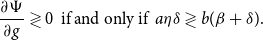 \begin{equation} \frac{\partial \Psi }{\partial g}\gtrless 0 \ \textrm{ if and only if } \ a\eta \delta \gtrless b(\beta +\delta ). \end{equation}
It follows that in response to a change in the output proportion of public spending, whether the resulting steady-state standard deviation of agents’ after-tax income is larger or smaller than that at the initial instant of time depends on the signs as well as strength of the associated long-run impacts on (i) the variability of relative capital stock as captured by $\frac{\partial \sigma _{\tilde{k}_{i}}}{\partial g}$
, and (ii) the aggregate labor hours adjusted by nongovernmental expenditure share
$\frac{\partial \sigma _{\tilde{k}_{i}}}{\partial g}$
, and (ii) the aggregate labor hours adjusted by nongovernmental expenditure share $(1-g)\tilde{H}$
as governed by
$(1-g)\tilde{H}$
as governed by $\frac{\partial \Psi }{\partial g}$
.
$\frac{\partial \Psi }{\partial g}$
.
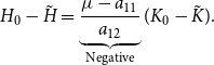
The underlying economic mechanism for the variability decomposition à la (47) can be understood as follows. Start our model from the original stationary allocations with $K_{0}=\tilde{K}$
and
$K_{0}=\tilde{K}$
and $H_{0}=\tilde{H}$
, as well as
$H_{0}=\tilde{H}$
, as well as $k_{i0}=$ $\tilde{k}_{i}$
for individual
$\tilde{k}_{i}$
for individual $i$
and then consider an increase in the GDP fraction of government purchases that generates the ensuing outcomes. First, since a larger government size raises the steady-state quantity of aggregate capital stock to a higher level denoted as
$i$
and then consider an increase in the GDP fraction of government purchases that generates the ensuing outcomes. First, since a larger government size raises the steady-state quantity of aggregate capital stock to a higher level denoted as $\hat{K}\gt$ $\tilde{K}$
[see equations (29) and (31)], the economy undertakes an expansion in capital accumulation along the transition path that will monotonically converge toward the long-run distribution of wealth/capital measured in terms of
$\tilde{K}$
[see equations (29) and (31)], the economy undertakes an expansion in capital accumulation along the transition path that will monotonically converge toward the long-run distribution of wealth/capital measured in terms of $\hat{k}_{i}\equiv \frac{\hat{K}_{i}}{\hat{K}}$
. In this case under a new public-spending share
$\hat{k}_{i}\equiv \frac{\hat{K}_{i}}{\hat{K}}$
. In this case under a new public-spending share $g^{\prime }$
, the beginning economy-wide amount of labor supply
$g^{\prime }$
, the beginning economy-wide amount of labor supply $H_{0}^{\prime }$
is larger than that at the new stationary state given by
$H_{0}^{\prime }$
is larger than that at the new stationary state given by $\hat{H}$
[see equation (36)], which in turn implies that the time-
$\hat{H}$
[see equation (36)], which in turn implies that the time- $0$
adjustment coefficient
$0$
adjustment coefficient $\Omega _{0}\gt 1$
per condition (43). It follows that as in (44), the resulting steady-state distribution of relative capital stock will be less unequal than the initial counterpart, that is,
$\Omega _{0}\gt 1$
per condition (43). It follows that as in (44), the resulting steady-state distribution of relative capital stock will be less unequal than the initial counterpart, that is, $\sigma _{\hat{k}_{i}}\lt \sigma _{k_{i0}}$
—this is dubbed as the wealth/capital inequality effect. Intuitively, after plugging the expression of
$\sigma _{\hat{k}_{i}}\lt \sigma _{k_{i0}}$
—this is dubbed as the wealth/capital inequality effect. Intuitively, after plugging the expression of $\phi _{i}$
from (39) into (41), we obtain that at
$\phi _{i}$
from (39) into (41), we obtain that at $t=0$
:
$t=0$
:
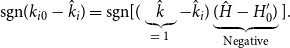 \begin{equation} \textrm{sgn}(k_{i0}-\hat{k}_{i})=\textrm{sgn}[(\underbrace{\hat{k}}_{=\textrm{ }1}-\hat{k}_{i})\underbrace{(\hat{H}-H_{0}^{\prime })}_{\textrm{Negative}}]. \end{equation}
For agents who possess the above-average level of aggregate wealth at the model’s new steady state $(\hat{k}_{i}\gt \hat{k})$
, the sign function of (50) shows that their relative capital stock will be decreasing on the convergent equilibrium trajectory with
$(\hat{k}_{i}\gt \hat{k})$
, the sign function of (50) shows that their relative capital stock will be decreasing on the convergent equilibrium trajectory with $k_{i0}\gt \hat{k}_{i}$
. On the contrary, (50) also yields that the relative wealth of individuals who end up with
$k_{i0}\gt \hat{k}_{i}$
. On the contrary, (50) also yields that the relative wealth of individuals who end up with $\hat{k}_{i}\lt \hat{k}$
will be increasing during the transition such that
$\hat{k}_{i}\lt \hat{k}$
will be increasing during the transition such that $k_{i0}\lt \hat{k}_{i}$
holds for these households. The aforementioned discussions altogether imply that the long-run distribution of wealth/capital will become less dispersed under a higher value of output share of public expenditures; hence,
$k_{i0}\lt \hat{k}_{i}$
holds for these households. The aforementioned discussions altogether imply that the long-run distribution of wealth/capital will become less dispersed under a higher value of output share of public expenditures; hence, $\frac{\partial \sigma _{\tilde{k}_{i}}}{\partial g}\lt 0$
.
$\frac{\partial \sigma _{\tilde{k}_{i}}}{\partial g}\lt 0$
.
Second, it is straightforward from the definition of $\Psi$
as shown in (45) to find that
$\Psi$
as shown in (45) to find that
 \begin{equation} \textrm{sgn}\left(\frac{\partial \Psi }{\partial g}\right)=\textrm{sgn}\left ( \frac{\partial \lbrack (1-g)\tilde{H}]}{\partial g}\right ), \end{equation}
where $\frac{\partial \Psi }{\partial g}$
is given by (48) with an indeterminate sign. This theoretical ambiguity is caused by two opposing forces generated from an increase in the public-spending share: a decrease in
$\frac{\partial \Psi }{\partial g}$
is given by (48) with an indeterminate sign. This theoretical ambiguity is caused by two opposing forces generated from an increase in the public-spending share: a decrease in $(1-g)$
versus a higher economy-wide level of hours worked in that
$(1-g)$
versus a higher economy-wide level of hours worked in that $\frac{\partial \tilde{H}}{\partial g}\gt 0$
à la (31)—this is dubbed as the adjusted-labor effect. It follows that it is uncertain a priori whether the long-run “adjusted” aggregate labor supply will rise or fall when the corresponding wealth/capital distribution becomes less unequal because of a higher
$\frac{\partial \tilde{H}}{\partial g}\gt 0$
à la (31)—this is dubbed as the adjusted-labor effect. It follows that it is uncertain a priori whether the long-run “adjusted” aggregate labor supply will rise or fall when the corresponding wealth/capital distribution becomes less unequal because of a higher $g$
, that is,
$g$
, that is, $\left ( 1-g^{\prime }\right ) \hat{H}\gtrless (1-g)\tilde{H}$
.
$\left ( 1-g^{\prime }\right ) \hat{H}\gtrless (1-g)\tilde{H}$
.
In sum, this subsection finds that upon an increase in the output proportion of government spending, the wealth/capital inequality effect always leads to a reduction in the long-run variability of relative capital stock, which in turn mitigates the extent of after-tax income inequality. Moreover, the adjusted-labor effect will further decrease $\sigma _{\tilde{y}_{i}^{a}}$
provided the necessary and sufficient condition for
$\sigma _{\tilde{y}_{i}^{a}}$
provided the necessary and sufficient condition for $\frac{\partial \Psi }{\partial g}\lt 0$
, given by (49), is satisfied. When these two effects are of opposite signs with
$\frac{\partial \Psi }{\partial g}\lt 0$
, given by (49), is satisfied. When these two effects are of opposite signs with $\frac{\partial \sigma _{\tilde{k}_{i}}}{\partial g}\lt 0$
and
$\frac{\partial \sigma _{\tilde{k}_{i}}}{\partial g}\lt 0$
and $\frac{\partial \Psi }{\partial g}\gt 0$
, the overall steady-state distributional impact of public expenditures on households’ disposal income is analytically ambiguous.
$\frac{\partial \Psi }{\partial g}\gt 0$
, the overall steady-state distributional impact of public expenditures on households’ disposal income is analytically ambiguous.
3.2. Quantitative analysis
In light of the inconclusive nature of the above theoretical analysis, this subsection undertakes a quantitative assessment on the long-run income-inequality effects of public spending within a calibrated version of our baseline macroeconomy. Specifically, the model is postulated to start at a stationary state with $K_{0}=\tilde{K}$
,
$K_{0}=\tilde{K}$
, $H_{0}=\tilde{H}$
, and
$H_{0}=\tilde{H}$
, and $k_{i0}=$ $\tilde{k}_{i}$
. For the benchmark parameterization, the capital and labor shares of national income,
$\tilde{k}_{i}$
. For the benchmark parameterization, the capital and labor shares of national income, $a$
and
$a$
and $b$
, are
$b$
, are $0.4$
and
$0.4$
and $0.6$
, respectively, the subjective rate of time preference
$0.6$
, respectively, the subjective rate of time preference $\beta$
is
$\beta$
is $0.04$
, the capital depreciation rate
$0.04$
, the capital depreciation rate $\delta$
is
$\delta$
is $0.06$
, the technological state
$0.06$
, the technological state $A$
and the fixed setup costs
$A$
and the fixed setup costs $Z$
under monopolistic competition are both normalized to
$Z$
under monopolistic competition are both normalized to $1$
, and the preference parameter
$1$
, and the preference parameter $\eta$
is set to be
$\eta$
is set to be $2.2951$
such that the initial steady-state level of aggregate labor hours is
$2.2951$
such that the initial steady-state level of aggregate labor hours is $0.3$
according to (28). As in García-Peñalosa and Turnovsky (Reference García-Peñalosa and Turnovsky2011), the beginning government size
$0.3$
according to (28). As in García-Peñalosa and Turnovsky (Reference García-Peñalosa and Turnovsky2011), the beginning government size $g$
is chosen to be
$g$
is chosen to be $0.15$
, and the IES associated with the household’s “effective consumption” à la (12) is selected to be
$0.15$
, and the IES associated with the household’s “effective consumption” à la (12) is selected to be $0.4$
, which in turn implies that
$0.4$
, which in turn implies that $\gamma =-1.5$
.
$\gamma =-1.5$
.
On the other hand, we note that $\frac{1}{\rho }$
is equal to the markup ratio of price over marginal cost with its empirical estimates ranging between
$\frac{1}{\rho }$
is equal to the markup ratio of price over marginal cost with its empirical estimates ranging between $1$
and
$1$
and $1.7$
; see Hall (Reference Hall1986), Domowitz et al. (Reference Domowitz, Hubbard and Petersen1988), Morrison (Reference Morrison1990) and Chirinko and Fazzari (Reference Chirinko and Fazzari1994), among others. It follows that the empirically plausible values of
$1.7$
; see Hall (Reference Hall1986), Domowitz et al. (Reference Domowitz, Hubbard and Petersen1988), Morrison (Reference Morrison1990) and Chirinko and Fazzari (Reference Chirinko and Fazzari1994), among others. It follows that the empirically plausible values of $\rho$
take on the interval
$\rho$
take on the interval $[0.59$
,
$[0.59$
, $1]$
. Moreover, (8) shows that the level of aggregate returns-to-scale in production is also given by
$1]$
. Moreover, (8) shows that the level of aggregate returns-to-scale in production is also given by $\frac{1}{\rho }$
. In this regard, Basu and Fernald (Reference Basu and Fernald1997, Table 3) present a point estimate of
$\frac{1}{\rho }$
. In this regard, Basu and Fernald (Reference Basu and Fernald1997, Table 3) present a point estimate of $1.03$
within the US private business economy, after correcting reallocation of productive inputs across industries, whereas Laitner and Stolyarov (Reference Laitner and Stolyarov2004) report a preferred range of 1.09–1.11 for the US economy. Based on these existing estimation results, the quantitative investigation below will explore parametric specifications with
$1.03$
within the US private business economy, after correcting reallocation of productive inputs across industries, whereas Laitner and Stolyarov (Reference Laitner and Stolyarov2004) report a preferred range of 1.09–1.11 for the US economy. Based on these existing estimation results, the quantitative investigation below will explore parametric specifications with $\rho =1$
(together with
$\rho =1$
(together with $Z=0$
for the perfectly competitive setting),
$Z=0$
for the perfectly competitive setting), $0.97$
and
$0.97$
and $0.9$
.
$0.9$
.
Our baseline measure of after-tax income inequality is calibrated to be the average Gini coefficient (based on disposable income, post taxes, and transfers) of USA, taken from OECD Income Distribution Database (2020), over the $2008$
–
$2008$
– $2017$
period. Accordingly,
$2017$
period. Accordingly, $Gini^{a}$
is set to be
$Gini^{a}$
is set to be $0.3876$
at the economy’s original stationary state.Footnote 12 We then use equation (46) to obtain the corresponding magnitude of
$0.3876$
at the economy’s original stationary state.Footnote 12 We then use equation (46) to obtain the corresponding magnitude of $\sigma _{\tilde{y}_{i}^{a}}\left ( =0.7165\right )$
, with which the initial steady-state standard deviation of relative capital stock can be derived from (45), specifically
$\sigma _{\tilde{y}_{i}^{a}}\left ( =0.7165\right )$
, with which the initial steady-state standard deviation of relative capital stock can be derived from (45), specifically $\sigma _{\tilde{k}_{i}}=2.506$
. Finally, under the maintained assumption that
$\sigma _{\tilde{k}_{i}}=2.506$
. Finally, under the maintained assumption that $k_{i0}=$ $\tilde{k}_{i}$
, condition (44) implies that the time-
$\tilde{k}_{i}$
, condition (44) implies that the time- $0$
adjustment coefficient
$0$
adjustment coefficient $\Omega _{0}=1$
for the benchmark calibration with
$\Omega _{0}=1$
for the benchmark calibration with $g=0.15$
.
$g=0.15$
.
3.2.1. Baseline results
Given the above-mentioned benchmark values of model parameters, Table 1 presents the steady-state effects on selected key macroeconomic aggregates as well as the wealth/capital and after-tax income inequalities of a 1% permanent increase in the output share of public expenditures. Its “ $g=0.15$
” columns present the beginning levels of these variables, together with the corresponding values of
$g=0.15$
” columns present the beginning levels of these variables, together with the corresponding values of $\Omega _{0}$
and
$\Omega _{0}$
and $\Psi$
, at the model’s original steady state under various degrees of market competitiveness, whereas the “
$\Psi$
, at the model’s original steady state under various degrees of market competitiveness, whereas the “ $g^{\prime }=0.16$
” columns report the resulting percentage changes relative to the initial counterparts. When
$g^{\prime }=0.16$
” columns report the resulting percentage changes relative to the initial counterparts. When $\rho =1$
and
$\rho =1$
and $Z=0$
, the economy’s production structure collapses to García-Peñalosa and Turnovsky’s (Reference García-Peñalosa and Turnovsky2011) perfectly competitive formulation with a single representative output-producing firm. Hence, equation (7) becomes degenerate, and we need to completely resolve this special case. As the monopolistic-markup parameter
$Z=0$
, the economy’s production structure collapses to García-Peñalosa and Turnovsky’s (Reference García-Peñalosa and Turnovsky2011) perfectly competitive formulation with a single representative output-producing firm. Hence, equation (7) becomes degenerate, and we need to completely resolve this special case. As the monopolistic-markup parameter $\rho$
decreases, our numerical simulations will ceteris paribus help gauge the quantitative importance of imperfect competition on income inequality.Footnote 13 Since the distributional effects of government spending are influenced by the dynamics of aggregate variables, the top six rows of Table 1 will display these impacts first.
$\rho$
decreases, our numerical simulations will ceteris paribus help gauge the quantitative importance of imperfect competition on income inequality.Footnote 13 Since the distributional effects of government spending are influenced by the dynamics of aggregate variables, the top six rows of Table 1 will display these impacts first.
Table 1. Benchmark model with useless government spending and $\gamma = -1.5$
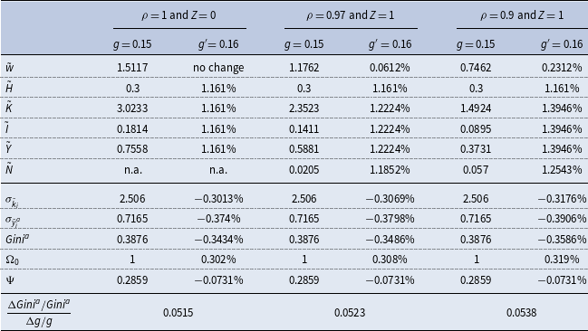
To understand the level effects shown in the upper portion of Table 1, we use the chain rule, combined with (8), (11), and (28)–(29), to find that the impact of a change in $g$
on the steady-state real wage rate
$g$
on the steady-state real wage rate $\tilde{w}$
is
$\tilde{w}$
is
 \begin{equation} \frac{\partial \tilde{w}}{\partial g}=\underbrace{\frac{(1-\rho )\tilde{w}}{(\rho -a)\tilde{H}}}_{=\textrm{ }\frac{\partial \tilde{w}}{\partial \tilde{H}}}\underbrace{\frac{\partial \tilde{H}}{\partial g}}_{\textrm{Positive}}, \end{equation}
where $a\lt \rho$
to ensure that our baseline model does not exhibit sustained endogenous growth à la (8), and
$a\lt \rho$
to ensure that our baseline model does not exhibit sustained endogenous growth à la (8), and $\frac{\partial \tilde{H}}{\partial g}$
is given by (31). It follows that
$\frac{\partial \tilde{H}}{\partial g}$
is given by (31). It follows that $\frac{\partial \tilde{w}}{\partial g}\gt \left ( =\right )$ $0$
when the markup ratio of price over marginal cost
$0$
when the markup ratio of price over marginal cost $\frac{1}{\rho }\gt \left ( =\right )$ $1$
. Intuitively, since the economy’s aggregate production function (8) displays constant returns-to-scale in
$1$
. Intuitively, since the economy’s aggregate production function (8) displays constant returns-to-scale in $K_{t}$
and
$K_{t}$
and $H_{t}$
under the perfectly competitive market structure (
$H_{t}$
under the perfectly competitive market structure ( $\rho =1$
and
$\rho =1$
and $Z=0$
), a higher labor supply shifting up the marginal product schedule for capital will increase investment and capital accumulation along the transition path. In the long run, there will be higher levels of aggregate capital and labor inputs, but the capital-to-labor ratio remains unchanged because of
$Z=0$
), a higher labor supply shifting up the marginal product schedule for capital will increase investment and capital accumulation along the transition path. In the long run, there will be higher levels of aggregate capital and labor inputs, but the capital-to-labor ratio remains unchanged because of $a+b=1$
; see Baxter and King (Reference Baxter and King1993, section III.B). It follows that capital, investment, and aggregate output all rise by the same percentage as labor hours
$a+b=1$
; see Baxter and King (Reference Baxter and King1993, section III.B). It follows that capital, investment, and aggregate output all rise by the same percentage as labor hours $\left ( =1.161\% \right )$
at the steady state. On the other hand, a constant long-run capital-to-labor ratio implies that the resulting relative factor price
$\left ( =1.161\% \right )$
at the steady state. On the other hand, a constant long-run capital-to-labor ratio implies that the resulting relative factor price $\frac{\tilde{w}}{\tilde{r}}$
is fixed. Since the steady-state capital rental rate
$\frac{\tilde{w}}{\tilde{r}}$
is fixed. Since the steady-state capital rental rate $\tilde{r}$ $( =\beta +\delta$
from equation (16) with
$( =\beta +\delta$
from equation (16) with $\dot{\lambda }_{it}=0)$
is invariant to movements in
$\dot{\lambda }_{it}=0)$
is invariant to movements in $g$
, the stationary level of real wage will not change either
$g$
, the stationary level of real wage will not change either $\left ( \frac{\partial \tilde{w}}{\partial g}=0\right )$
.
$\left ( \frac{\partial \tilde{w}}{\partial g}=0\right )$
.
In our monopolistically competitive specifications with $\rho \in (0$
,
$\rho \in (0$
, $1)$
and
$1)$
and $Z=1$
, just like the aforementioned discussions under perfect competition, a larger government size raises the long-run labor hours, capital stock, gross investment, and total output. However, their quantitative results are quite different, since more entries of intermediate-goods-producing firms will take place as per equation (7). Using (8) shows that the economy with
$Z=1$
, just like the aforementioned discussions under perfect competition, a larger government size raises the long-run labor hours, capital stock, gross investment, and total output. However, their quantitative results are quite different, since more entries of intermediate-goods-producing firms will take place as per equation (7). Using (8) shows that the economy with $\rho =0.97$
exhibits a higher aggregate output elasticity with respect to hours worked than that with
$\rho =0.97$
exhibits a higher aggregate output elasticity with respect to hours worked than that with $\rho =1$
, which in turn generates an endogenous enhancement of the steady-state labor productivity
$\rho =1$
, which in turn generates an endogenous enhancement of the steady-state labor productivity $\frac{\tilde{Y}}{\tilde{H}}$
. It follows from equation (11) that the real wage rate will rise (by
$\frac{\tilde{Y}}{\tilde{H}}$
. It follows from equation (11) that the real wage rate will rise (by $0.0612$
%) in the long run. In addition, given the parametric restriction of
$0.0612$
%) in the long run. In addition, given the parametric restriction of $a\lt \rho$
, a higher stationary level of economy-wide labor supply (by
$a\lt \rho$
, a higher stationary level of economy-wide labor supply (by $1.161$
%) leads to a more than proportional increase in the aggregate capital stock (by
$1.161$
%) leads to a more than proportional increase in the aggregate capital stock (by $1.2224$
%; see equation (29)) and the measure of intermediate-input firms (by
$1.2224$
%; see equation (29)) and the measure of intermediate-input firms (by $1.1852$
%). Finally, to maintain the constant capital rental rate at the steady state à la (10), total output will be increased by the same percentage as the capital stock in the long run.
$1.1852$
%). Finally, to maintain the constant capital rental rate at the steady state à la (10), total output will be increased by the same percentage as the capital stock in the long run.
In terms of the dispersion/inequality responses reported in the bottom portion of Table 1, we first note that the benchmark parameterization of $\{a$
,
$\{a$
, $b$
,
$b$
, $\beta$
,
$\beta$
, $\delta$
,
$\delta$
, $\eta \}$
described above satisfies the requisite condition (49) for
$\eta \}$
described above satisfies the requisite condition (49) for $\frac{\partial \Psi }{\partial g}\lt 0$
. In particular, the scaling parameter
$\frac{\partial \Psi }{\partial g}\lt 0$
. In particular, the scaling parameter $\Psi$
falls by
$\Psi$
falls by $0.0731$
% when the government size increases to
$0.0731$
% when the government size increases to $g^{\prime }=0.16$
within each parametric configuration under consideration. Per the decomposition equation (47), it follows that both the (unambiguously negative) wealth/capital inequality effect and the adjusted-labor effect will decrease the steady-state standard deviation of agents’ disposable income; hence, an increase in government purchases leads to a lower degree of after-tax income inequality. However, the resulting long-run reduction in income inequality is quantitatively small. For the most parsimonious formulation with perfect competition (
$g^{\prime }=0.16$
within each parametric configuration under consideration. Per the decomposition equation (47), it follows that both the (unambiguously negative) wealth/capital inequality effect and the adjusted-labor effect will decrease the steady-state standard deviation of agents’ disposable income; hence, an increase in government purchases leads to a lower degree of after-tax income inequality. However, the resulting long-run reduction in income inequality is quantitatively small. For the most parsimonious formulation with perfect competition ( $\rho =1$
and
$\rho =1$
and $Z=0$
), we find that a 1% expansion in the public-spending share will yield a decrease in
$Z=0$
), we find that a 1% expansion in the public-spending share will yield a decrease in $Gini^{a}$
by
$Gini^{a}$
by $0.3434\%$
, which in turn leads to a calculated elasticity (shown in the last row of Table 1) of
$0.3434\%$
, which in turn leads to a calculated elasticity (shown in the last row of Table 1) of $0.0515$
. This figure is significantly lower than the estimated range of 0.22–0.38 reported by Doerrenberg and Peichl (Reference Doerrenberg and Peichl2014) and Guzi and Kahanec (Reference Guzi and Kahanec2018).
$0.0515$
. This figure is significantly lower than the estimated range of 0.22–0.38 reported by Doerrenberg and Peichl (Reference Doerrenberg and Peichl2014) and Guzi and Kahanec (Reference Guzi and Kahanec2018).
With an imperfectly competitive production structure, Table 1 shows that the associated adjusted-labor effect (represented by $\frac{\Delta \Psi }{\Psi }=-0.0731\%$
) is quantitatively independent of the calibrated values for
$\frac{\Delta \Psi }{\Psi }=-0.0731\%$
) is quantitatively independent of the calibrated values for $\rho$
because it does not enter the expression of
$\rho$
because it does not enter the expression of $\tilde{H}$
or
$\tilde{H}$
or $\Psi$
. Moreover, as discussed earlier, the percentage increase in the long-run aggregate capital stock gets larger when the monopolistic-markup parameter
$\Psi$
. Moreover, as discussed earlier, the percentage increase in the long-run aggregate capital stock gets larger when the monopolistic-markup parameter $\rho$
falls further. It follows that the economy’s speed of convergence toward the new steady state will be slowed down, which in turn enhances the declining dispersion of agents’ relative capital distribution along the transition path. As a result, the wealth/capital inequality effect becomes stronger, since the absolute value for the percentage reduction in
$\rho$
falls further. It follows that the economy’s speed of convergence toward the new steady state will be slowed down, which in turn enhances the declining dispersion of agents’ relative capital distribution along the transition path. As a result, the wealth/capital inequality effect becomes stronger, since the absolute value for the percentage reduction in $\sigma _{\tilde{k}_{i}}$
rises with a higher degree of monopoly market power. The preceding analysis thus implies that upon an increase in the government size within our benchmark parameterization, the decrease in after-tax income inequality or
$\sigma _{\tilde{k}_{i}}$
rises with a higher degree of monopoly market power. The preceding analysis thus implies that upon an increase in the government size within our benchmark parameterization, the decrease in after-tax income inequality or $Gini^{a}$
will be ceteris paribus larger under imperfect competition than that for the corresponding perfectly competitive formulation. Nevertheless, the resulting elasticities of after-tax Gini with respect to public expenditures (
$Gini^{a}$
will be ceteris paribus larger under imperfect competition than that for the corresponding perfectly competitive formulation. Nevertheless, the resulting elasticities of after-tax Gini with respect to public expenditures ( $0.0523$
when
$0.0523$
when $\rho =0.97$
and
$\rho =0.97$
and $0.0538$
when
$0.0538$
when $\rho =0.9$
) remain too low to be empirically realistic. In sum, we have found that in the context of our baseline macroeconomy, monopolistic competition alone does not help deliver a quantitative match with the actual data on the long-run distributional consequences of government spending.
$\rho =0.9$
) remain too low to be empirically realistic. In sum, we have found that in the context of our baseline macroeconomy, monopolistic competition alone does not help deliver a quantitative match with the actual data on the long-run distributional consequences of government spending.
3.2.2 Sensitivity analysis
With regard to the sensitivity analysis, we find that the simulation results reported in Table 1 remain quantitatively robust to changes in $\{a$
,
$\{a$
, $b$
,
$b$
, $\beta$
,
$\beta$
, $\delta$
,
$\delta$
, $\eta$
,
$\eta$
, $g\}$
over their respective empirically plausible ranges, as well as to different initial values of
$g\}$
over their respective empirically plausible ranges, as well as to different initial values of $\{Gini^{a}$
,
$\{Gini^{a}$
, $\sigma _{\tilde{y}_{i}^{a}}$
,
$\sigma _{\tilde{y}_{i}^{a}}$
, $\sigma _{\tilde{k}_{i}}\}$
. For each household’s IES (IES
$\sigma _{\tilde{k}_{i}}\}$
. For each household’s IES (IES $=\frac{1}{1-\gamma }$
), many previous studies have adopted the interval of
$=\frac{1}{1-\gamma }$
), many previous studies have adopted the interval of $[\frac{1}{3}$
,
$[\frac{1}{3}$
, $1]$
in their quantitative investigation, so does our baseline parameterization with
$1]$
in their quantitative investigation, so does our baseline parameterization with $\gamma =-1.5$
. However, some empirical research suggests that the elasticity of intertemporal consumption substitution is higher than 1. For example, Vissing-Jørgensen and Attanasio (Reference Vissing-Jørgensen and Attanasio2003) report the point estimates of IES to be
$\gamma =-1.5$
. However, some empirical research suggests that the elasticity of intertemporal consumption substitution is higher than 1. For example, Vissing-Jørgensen and Attanasio (Reference Vissing-Jørgensen and Attanasio2003) report the point estimates of IES to be $1.03$
(with six instruments) and
$1.03$
(with six instruments) and $1.44$
(under one instrumental variable) for the group of all stock holders. Gruber (Reference Gruber2013) finds that the IES is around
$1.44$
(under one instrumental variable) for the group of all stock holders. Gruber (Reference Gruber2013) finds that the IES is around $2$
when endogenous tax rate movements are included in his cross-sectional estimation on US total nondurable consumption expenditures, and that this result is in line with Mulligan’s (Reference Mulligan2002) earlier estimates based on time series data of total returns to capital. Drawing on these estimation findings, Table 2 presents numerical results of our model economy under alternative calibrations with
$2$
when endogenous tax rate movements are included in his cross-sectional estimation on US total nondurable consumption expenditures, and that this result is in line with Mulligan’s (Reference Mulligan2002) earlier estimates based on time series data of total returns to capital. Drawing on these estimation findings, Table 2 presents numerical results of our model economy under alternative calibrations with $\gamma =-1$
(IES
$\gamma =-1$
(IES $=0.5$
);
$=0.5$
); $\gamma =0$
(IES
$\gamma =0$
(IES $=1$
); hence, the instantaneous utility function (12) is separable and logarithmic in consumption and leisure, and
$=1$
); hence, the instantaneous utility function (12) is separable and logarithmic in consumption and leisure, and $\gamma =0.4$
(IES
$\gamma =0.4$
(IES $=1.67$
), which is close to its highest possible value that satisfies the requisite condition
$=1.67$
), which is close to its highest possible value that satisfies the requisite condition $\gamma \eta \lt 1$
for the preference concavity in leisure.
$\gamma \eta \lt 1$
for the preference concavity in leisure.
Table 2. Benchmark model with useless government spending: sensitivity analysis under $\gamma = \{-1, 0, 0.4\}$
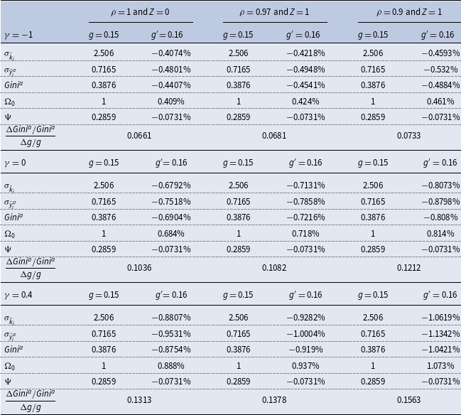
We note that since the steady-state expressions of aggregate labor hours $\tilde{H}$
and capital stock
$\tilde{H}$
and capital stock $\tilde{K}$
[see equations (28) and (29)], as well as the remaining economy-wide variables
$\tilde{K}$
[see equations (28) and (29)], as well as the remaining economy-wide variables $\{\tilde{w}$
,
$\{\tilde{w}$
, $\tilde{I}$
,
$\tilde{I}$
, $\tilde{Y}$
,
$\tilde{Y}$
, $\tilde{N}\}$
, are independent of changes in agents’ intertemporal elasticity of consumption substitution, the associated level effects from a higher public-spending share are quantitatively identical to those shown in the top six rows of Table 1. Accordingly, Table 2 will focus exclusively on the corresponding dispersion/inequality responses. It turns out that the magnitude of the adjusted-labor effect remains unchanged, that is,
$\tilde{N}\}$
, are independent of changes in agents’ intertemporal elasticity of consumption substitution, the associated level effects from a higher public-spending share are quantitatively identical to those shown in the top six rows of Table 1. Accordingly, Table 2 will focus exclusively on the corresponding dispersion/inequality responses. It turns out that the magnitude of the adjusted-labor effect remains unchanged, that is, $\frac{\Delta \Psi }{\Psi }=-0.0731\%$
, because variations of
$\frac{\Delta \Psi }{\Psi }=-0.0731\%$
, because variations of $\gamma$
do not affect the scaling parameter
$\gamma$
do not affect the scaling parameter $\Psi$
given by (45). On the other hand, a higher
$\Psi$
given by (45). On the other hand, a higher $\gamma$
or IES strengthens the intertemporal substitution effect of consumption across different instants of time, which in turn will reduce the accumulation rate of aggregate capital stock toward the new stationary state
$\gamma$
or IES strengthens the intertemporal substitution effect of consumption across different instants of time, which in turn will reduce the accumulation rate of aggregate capital stock toward the new stationary state $\hat{K}$
upon an expansion in
$\hat{K}$
upon an expansion in $g$
.Footnote 14 We numerically verify this result by finding
$g$
.Footnote 14 We numerically verify this result by finding $\frac{\partial \left \vert \mu \right \vert }{\partial \gamma }\lt 0$
, indicating that the stable eigenvalue’s modulus becomes smaller as the IES rises. Table 2 thus shows that when the government size is increased to
$\frac{\partial \left \vert \mu \right \vert }{\partial \gamma }\lt 0$
, indicating that the stable eigenvalue’s modulus becomes smaller as the IES rises. Table 2 thus shows that when the government size is increased to $g^{\prime }=0.16$
within each parametric specification, the resulting percentage increases of the adjustment coefficient, given by (43) with
$g^{\prime }=0.16$
within each parametric specification, the resulting percentage increases of the adjustment coefficient, given by (43) with $\frac{\partial \Omega _{0}}{\partial \left \vert \mu \right \vert }\lt 0$
, are ceteris paribus monotonically increasing with respect to
$\frac{\partial \Omega _{0}}{\partial \left \vert \mu \right \vert }\lt 0$
, are ceteris paribus monotonically increasing with respect to $\gamma$
. Using equations (44)–(46), it follows that the steady-state standard deviations of relative capital stock and after-tax income, as well as the Gini coefficient, will all fall further because of a stronger wealth/capital inequality effect.Footnote 15 Under
$\gamma$
. Using equations (44)–(46), it follows that the steady-state standard deviations of relative capital stock and after-tax income, as well as the Gini coefficient, will all fall further because of a stronger wealth/capital inequality effect.Footnote 15 Under $\rho =0.9$
and
$\rho =0.9$
and $\gamma =0.4$
, these outcomes in turn raise the calculated elasticity to
$\gamma =0.4$
, these outcomes in turn raise the calculated elasticity to $0.1563$
(shown in the last row of Table 2), which is still unrealistically low vis-à-vis estimation results of previous econometric studies.
$0.1563$
(shown in the last row of Table 2), which is still unrealistically low vis-à-vis estimation results of previous econometric studies.
4. Useful Government Spending
In the context of our baseline model studied above, government purchases are postulated to yield no substitution effects in that they do not influence the marginal conditions associated with the households’ consumption/savings nor the firms’ production decisions. However, the assumption of wasteful public spending, although commonly adopted in the academic literature for analytical simplicity, is not necessarily the most realistic—at least within USA and many developed countries. In this section, we will examine an identical monopolistically competitive macroeconomy, but with useful government expenditures on goods and services. On the economy’s supply side, government spending may enter the representative final-good producer’s production technology (1) as an externality that is complementary to intermediate inputs à la Barro (Reference Barro1990). On the economy’s demand side, public expenditure may enter household $i$
’s utility function (12) nonseparably as a positive preference externality à la García-Peñalosa and Turnovsky (Reference García-Peñalosa and Turnovsky2011). In what follows, numerical experiments are conducted to quantitatively assess the long-run distributional effects on agents’ after-tax income under either productive or utility-generating government purchases within our model economy.
$i$
’s utility function (12) nonseparably as a positive preference externality à la García-Peñalosa and Turnovsky (Reference García-Peñalosa and Turnovsky2011). In what follows, numerical experiments are conducted to quantitatively assess the long-run distributional effects on agents’ after-tax income under either productive or utility-generating government purchases within our model economy.
4.1. Productive Government Spending
In this case, a single homogeneous final output is produced by the following technology:
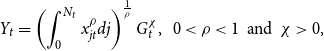 \begin{equation} Y_{t}=\left ( \int _{0}^{N_{t}}x_{jt}^{\rho }dj\right ) ^{\frac{1}{\rho }}G_{t}^{\chi },\textrm{ }\ 0\lt \rho \lt 1 \ \textrm{ and }\ \chi \gt 0, \end{equation}
where $\chi$
captures the degree of positive external effects that government expenditures exert on the final-good firm’s production process. Next, we follow the same solution procedure as in Section 2 to find that (i) the economy’s aggregate technology now becomes
$\chi$
captures the degree of positive external effects that government expenditures exert on the final-good firm’s production process. Next, we follow the same solution procedure as in Section 2 to find that (i) the economy’s aggregate technology now becomes
 \begin{equation} Y_{t}=\left [ \rho A^{\frac{1}{\rho }}g^{\chi }\left ( \frac{1-\rho }{Z}\right ) ^{\frac{1-\rho }{\rho }}K_{t}^{\frac{a}{\rho }}H_{t}^{\frac{b}{\rho }}\right ] ^{\frac{1}{1-\chi }}, \end{equation}
where $\frac{a}{\rho (1-\chi )}$ $\lt 1$
to eliminate the occurrence of persistent economic growth, and the resulting level of aggregate returns-to-scale in total capital and labor inputs is equal to
$\lt 1$
to eliminate the occurrence of persistent economic growth, and the resulting level of aggregate returns-to-scale in total capital and labor inputs is equal to $\frac{1}{\rho (1-\chi )}$
, which is higher than that of (8) under useless public spending; (ii) the autonomous pair of differential equations that govern the dynamic trajectories of
$\frac{1}{\rho (1-\chi )}$
, which is higher than that of (8) under useless public spending; (ii) the autonomous pair of differential equations that govern the dynamic trajectories of $K_{t}$
and
$K_{t}$
and $H_{t}$
are
$H_{t}$
are
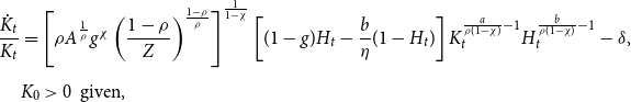 \begin{align} \frac{\dot{K}_{t}}{K_{t}}&=\left [ \rho A^{\frac{1}{\rho }}g^{\chi }\left ( \frac{1-\rho }{Z}\right ) ^{\frac{1-\rho }{\rho }}\right ] ^{\frac{1}{1-\chi }}\left [ (1-g)H_{t}-\frac{b}{\eta }(1-H_{t})\right ] K_{t}^{\frac{a}{\rho (1-\chi )}-1}H_{t}^{\frac{b}{\rho (1-\chi )}-1}-\delta,\nonumber \\[5pt] & K_{0}\gt 0\ \textrm{ given,} \end{align}
 \begin{equation} \frac{\dot{H}_{t}}{H_{t}}=\frac{\beta +\delta +\left [ \frac{a(1-\gamma )}{\rho (1-\chi )}\right ] \frac{\dot{K}_{t}}{K_{t}}-\frac{a}{K_{t}}\left [ \rho A^{\frac{1}{\rho }}g^{\chi }\left ( \frac{1-\rho }{Z}\right ) ^{\frac{1-\rho }{\rho }}K_{t}^{\frac{a}{\rho }}H_{t}^{\frac{b}{\rho }}\right ] ^{\frac{1}{1-\chi }}}{(1-\gamma )[1-\frac{b}{\rho (1-\chi )}]+[1-\gamma (1+\eta )]\left ( \frac{H_{t}}{1-H_{t}}\right ) }; \end{equation}
and (iii) the necessary and sufficient condition for saddle-path stability is given by:
 \begin{equation} \chi \lt \underbrace{1-\frac{b\eta (1-\gamma )[(b-g)\delta +(1-g)\beta ]}{\rho \left \{ \eta (1-\gamma )[(b-g)\delta +(1-g)\beta ]+b(\beta +\delta )[1-\gamma (1+\eta )]\right \} }}_{\equiv \textrm{ }\chi ^{\max }}. \end{equation}
Based on existing empirical estimates for the output elasticity of government spending that range from $0.03$
(Eberts, Reference Eberts1986) to
$0.03$
(Eberts, Reference Eberts1986) to $0.39$
(Aschauer, Reference Aschauer1989), a “conservative” figure of
$0.39$
(Aschauer, Reference Aschauer1989), a “conservative” figure of $\chi =0.1$
is adopted in our subsequent quantitative analyses. Table 3 presents the resulting dispersion and inequality effects under identical calibrations of
$\chi =0.1$
is adopted in our subsequent quantitative analyses. Table 3 presents the resulting dispersion and inequality effects under identical calibrations of $\{a$
,
$\{a$
, $b$
,
$b$
, $\beta$
,
$\beta$
, $\delta$
,
$\delta$
, $\eta \}$
as in the benchmark model, together with the monopolistic-markup parameter
$\eta \}$
as in the benchmark model, together with the monopolistic-markup parameter $\rho =\{1$
,
$\rho =\{1$
, $0.97$
,
$0.97$
, $0.9\}$
and the household’s IES
$0.9\}$
and the household’s IES $\gamma =\{-1$
,
$\gamma =\{-1$
, $0$
,
$0$
, $0.4\}$
, for ease of comparative comparisons with Table 2.Footnote 16
$0.4\}$
, for ease of comparative comparisons with Table 2.Footnote 16
Table 3. Productive government spending with $\chi = 0.1$
and
$\chi = 0.1$
and $ \gamma = \{-1, 0, 0.4\}$
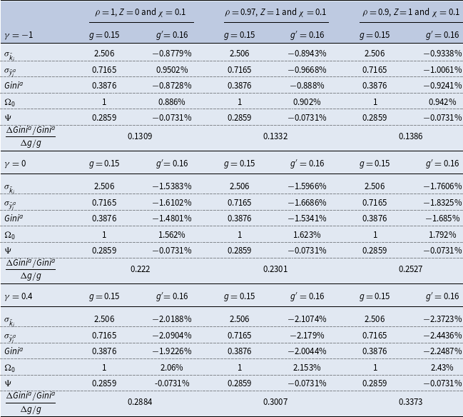
We first note that since the scaling parameter $\Psi$
defined in (45) is independent of
$\Psi$
defined in (45) is independent of $\chi$
, the magnitude of the adjusted-labor effect will remain unaffected (given by
$\chi$
, the magnitude of the adjusted-labor effect will remain unaffected (given by $\frac{\Delta \Psi }{\Psi }=-0.0731\%$
) upon an expansion in the government size across Tables 2 and 3. In addition, while keeping the values of other parameters the same, the percentage changes reported in the remaining “
$\frac{\Delta \Psi }{\Psi }=-0.0731\%$
) upon an expansion in the government size across Tables 2 and 3. In addition, while keeping the values of other parameters the same, the percentage changes reported in the remaining “ $g^{\prime }=0.16$
” cells, as well as the calculated elasticities, of Table 3 under
$g^{\prime }=0.16$
” cells, as well as the calculated elasticities, of Table 3 under $\chi =0.1$
are all larger (in absolute terms) than those corresponding to Table 2 with
$\chi =0.1$
are all larger (in absolute terms) than those corresponding to Table 2 with $\chi =0$
. Intuitively, although adding productive public expenditures does not affect the steady-state aggregate labor hours
$\chi =0$
. Intuitively, although adding productive public expenditures does not affect the steady-state aggregate labor hours $\tilde{H}$
per equation (28), the associated economy-wide level of capital stock is changed to
$\tilde{H}$
per equation (28), the associated economy-wide level of capital stock is changed to
 \begin{equation} \tilde{K}=\left \{ A\left ( \frac{1-\rho }{Z}\right ) ^{1-\rho }\left [ \rho g^{\chi }\left ( \frac{a}{\beta +\delta }\right ) ^{1-\chi }\right ] ^{\rho }\tilde{H}^{b}\right \} ^{\frac{1}{\rho \left ( 1-\chi \right ) -a}}. \end{equation}
It follows that a higher $g$
will raise the long-run total labor supply by the same proportion under either useless or productivity-augmenting government spending [see equation (31)]. However, a side-by-side comparison of (29) versus (58) yields that this equalized increase in
$g$
will raise the long-run total labor supply by the same proportion under either useless or productivity-augmenting government spending [see equation (31)]. However, a side-by-side comparison of (29) versus (58) yields that this equalized increase in $\tilde{H}$
leads to a larger response of the stationary-state aggregate capital stock (in percentage term) when
$\tilde{H}$
leads to a larger response of the stationary-state aggregate capital stock (in percentage term) when $\chi =0.1$
, because the relevant elasticity exponent
$\chi =0.1$
, because the relevant elasticity exponent $\frac{1}{\rho \left ( 1-\chi \right ) -a}\gt \frac{1}{\rho -a}$
when
$\frac{1}{\rho \left ( 1-\chi \right ) -a}\gt \frac{1}{\rho -a}$
when $0\lt \chi \lt 1-\frac{a}{\rho }$
to rule out the possibility of sustained endogenous growth. This outcome decreases the capital accumulation rate in that the economy’s convergence speed toward the new steady state (reflected by
$0\lt \chi \lt 1-\frac{a}{\rho }$
to rule out the possibility of sustained endogenous growth. This outcome decreases the capital accumulation rate in that the economy’s convergence speed toward the new steady state (reflected by $\frac{\partial \left \vert \mu \right \vert }{\partial \chi }\lt 0$
) along the stable arm of the equilibrium saddle path will be slowed down. As a result, the percentage increases in the time-
$\frac{\partial \left \vert \mu \right \vert }{\partial \chi }\lt 0$
) along the stable arm of the equilibrium saddle path will be slowed down. As a result, the percentage increases in the time- $0$
adjustment coefficient
$0$
adjustment coefficient $\Omega _{0}$
shown in Table 3 are higher than those in the matching parameterizations of Table 2. This implies that as
$\Omega _{0}$
shown in Table 3 are higher than those in the matching parameterizations of Table 2. This implies that as $\chi$
rises, the long-run distribution of relative capital stock will ceteris paribus become less unequal because of a stronger wealth/capital inequality effect: the absolute value for the percentage reduction in
$\chi$
rises, the long-run distribution of relative capital stock will ceteris paribus become less unequal because of a stronger wealth/capital inequality effect: the absolute value for the percentage reduction in $\sigma _{\tilde{k}_{i}}$
is monotonically increasing with the output elasticity of public expenditures. Consequently, the posttax income inequality
$\sigma _{\tilde{k}_{i}}$
is monotonically increasing with the output elasticity of public expenditures. Consequently, the posttax income inequality $\sigma _{\tilde{y}_{i}^{a}}$
and Gini coefficient
$\sigma _{\tilde{y}_{i}^{a}}$
and Gini coefficient $Gini^{a}$
are going to fall further as well.
$Gini^{a}$
are going to fall further as well.
In the context of a perfectly competitive macroeconomy ( $\rho =1$
and
$\rho =1$
and $Z=0$
), Table 3 shows that under the log-log utility function with
$Z=0$
), Table 3 shows that under the log-log utility function with $\gamma =0$
and useful public spending with
$\gamma =0$
and useful public spending with $\chi =0.1$
, a 1% expansion of
$\chi =0.1$
, a 1% expansion of $g$
will generate a decrease in
$g$
will generate a decrease in $Gini^{a}$
by
$Gini^{a}$
by $1.4801\%$
. This in turn leads to a calculated elasticity of
$1.4801\%$
. This in turn leads to a calculated elasticity of $0.222$
, which is just slightly above the lower bound of the estimated interval
$0.222$
, which is just slightly above the lower bound of the estimated interval $[0.22$
,
$[0.22$
, $0.38]$
that Doerrenberg and Peichl (Reference Doerrenberg and Peichl2014) and Guzi and Kahanec (Reference Guzi and Kahanec2018) have obtained. It follows that incorporating productive government expenditure alone into García-Peñalosa and Turnovsky’s (Reference García-Peñalosa and Turnovsky2011) Ramsey model (without deviating from perfect competition) is able to deliver a rather marginal quantitative match with the actual data on the long-run distributional impact of government purchases. Moreover, as discussed in Section 3, since an increase in the monopolistic market power (smaller
$0.38]$
that Doerrenberg and Peichl (Reference Doerrenberg and Peichl2014) and Guzi and Kahanec (Reference Guzi and Kahanec2018) have obtained. It follows that incorporating productive government expenditure alone into García-Peñalosa and Turnovsky’s (Reference García-Peñalosa and Turnovsky2011) Ramsey model (without deviating from perfect competition) is able to deliver a rather marginal quantitative match with the actual data on the long-run distributional impact of government purchases. Moreover, as discussed in Section 3, since an increase in the monopolistic market power (smaller $\rho$
) or each household’s intertemporal elasticity of consumption substitution (higher
$\rho$
) or each household’s intertemporal elasticity of consumption substitution (higher $\gamma$
) strengthens the wealth/capital inequality effect, the resulting elasticities of after-tax Gini with respect to public expenditures will be higher (
$\gamma$
) strengthens the wealth/capital inequality effect, the resulting elasticities of after-tax Gini with respect to public expenditures will be higher ( $0.2527$
when
$0.2527$
when $\rho =0.9$
and
$\rho =0.9$
and $\gamma =0$
;
$\gamma =0$
; $0.2884$
when
$0.2884$
when $\rho =1$
and
$\rho =1$
and $\gamma =0.4$
; and
$\gamma =0.4$
; and $0.3373$
when
$0.3373$
when $\rho =0.9$
and
$\rho =0.9$
and $\gamma =0.4$
) and thus provide a much closer fit with recent estimation results.
$\gamma =0.4$
) and thus provide a much closer fit with recent estimation results.
4.2. Utility-generating government spending
In this case, household $i$
’s discounted lifetime utilities are modified to
$i$
’s discounted lifetime utilities are modified to
 \begin{equation} \int _{0}^{\infty }\underbrace{\frac{1}{\gamma }\left ( C_{it}\ell _{it}^{\eta }G_{t}^{\theta }\right ) ^{\gamma }}_{\equiv \textrm{ }U_{it}}e^{-\beta t}dt,\, \,-\infty \lt \gamma \lt 1, \eta,\textrm{ }\theta,\textrm{ }\beta \gt 0,\, \, \textrm{and}\gamma \eta \lt 1, \end{equation}
where $\theta$
represents the degree of a positive preference externality that government spending exerts on the composite good
$\theta$
represents the degree of a positive preference externality that government spending exerts on the composite good $C_{it}\ell _{it}^{\eta }$
. When
$C_{it}\ell _{it}^{\eta }$
. When $\gamma =0$
, the time-
$\gamma =0$
, the time- $t$
utility function
$t$
utility function $U_{it}$
exhibits additive separability between private consumption, leisure, and public good; hence, the marginal utilities of
$U_{it}$
exhibits additive separability between private consumption, leisure, and public good; hence, the marginal utilities of $C_{t}$
and
$C_{t}$
and $\ell _{t}$
are independent of
$\ell _{t}$
are independent of $G_{t}$
. When
$G_{t}$
. When $\gamma \gt \left ( \lt \right )$ $0$
, the marginal utility of private consumption increases (decreases) with respect to government purchases; thus,
$0$
, the marginal utility of private consumption increases (decreases) with respect to government purchases; thus, $C_{t}$
and
$C_{t}$
and $G_{t}$
are Edgeworth complements (substitutes).
$G_{t}$
are Edgeworth complements (substitutes).
It is then straightforward to derive that (i) all the first-order conditions that characterize firms’ production decisions and factor demands, as shown in Section 2.1, will remain unaffected; (ii) the steady-state quantities of aggregate labor hours and capital stock, given by (28)–(29), are independent of the preference-externality parameter $\theta$
; and (iii) the autonomous pair of differential equations that determine the dynamic evolutions of
$\theta$
; and (iii) the autonomous pair of differential equations that determine the dynamic evolutions of $K_{t}$
and
$K_{t}$
and $H_{t}$
are equation (26) and
$H_{t}$
are equation (26) and
 \begin{equation} \frac{\dot{H}_{t}}{H_{t}}=\frac{\beta +\delta +\left [ \frac{a(1-\gamma -\theta \gamma )}{\rho }\right ] \frac{\dot{K}_{t}}{K_{t}}-\rho aA^{\frac{1}{\rho }}\left ( \frac{1-\rho }{Z}\right ) ^{\frac{1-\rho }{\rho }}K_{t}^{\frac{a}{\rho }-1}H_{t}^{\frac{b}{\rho }}}{\frac{b\theta \gamma }{\rho }+(1-\gamma )(1-\frac{b}{\rho })+[1-\gamma (1+\eta )]\left ( \frac{H_{t}}{1-H_{t}}\right ) }. \end{equation}
We also find that given $\theta \gt 0$
, this economy’s unique interior steady state always displays local determinacy over the interval
$\theta \gt 0$
, this economy’s unique interior steady state always displays local determinacy over the interval $\gamma \in \lbrack 0$
,
$\gamma \in \lbrack 0$
, $1)$
, and that the necessary and sufficient condition for saddle-path stability with
$1)$
, and that the necessary and sufficient condition for saddle-path stability with $\gamma \lt 0$
is
$\gamma \lt 0$
is
 \begin{equation} \theta \lt \underbrace{\frac{(\rho -b)(1-\frac{1}{\gamma })[(b-g)\delta +(1-g)\beta ]+\frac{\rho b(\beta +\delta )}{\eta }(1+\eta -\frac{1}{\gamma })}{b[(b-g)\delta +(1-g)\beta ]}}_{\equiv \textrm{ }\theta ^{\max }}. \end{equation}
Using García-Peñalosa and Turnovsky’s (Reference García-Peñalosa and Turnovsky2011) calibration of $\theta =0.3$
, Table 4 presents the associated dispersion/inequality effects under the same selected values of
$\theta =0.3$
, Table 4 presents the associated dispersion/inequality effects under the same selected values of $\{a$
,
$\{a$
, $b$
,
$b$
, $\beta$
,
$\beta$
, $\delta$
,
$\delta$
, $\eta \}$
per the baseline parameterization, in conjunction with
$\eta \}$
per the baseline parameterization, in conjunction with $\rho =\{1$
,
$\rho =\{1$
, $0.97$
,
$0.97$
, $0.9\}$
and
$0.9\}$
and $\gamma =\{-1$
,
$\gamma =\{-1$
, $0$
,
$0$
, $0.4\}$
. We first note that as the preference formulation (59) become logarithmically separable in private consumption and public good (
$0.4\}$
. We first note that as the preference formulation (59) become logarithmically separable in private consumption and public good ( $\gamma =0$
), the inclusion of utility-enhancing government purchases does not yield any impact on the model’s equilibrium conditions and distributional dynamics. It follows that the numerical results reported in Tables 2 and 4 are identical when the household’s IES is equal to
$\gamma =0$
), the inclusion of utility-enhancing government purchases does not yield any impact on the model’s equilibrium conditions and distributional dynamics. It follows that the numerical results reported in Tables 2 and 4 are identical when the household’s IES is equal to $1$
. On the other hand, since
$1$
. On the other hand, since $\theta$
does not enter the expression for the scaling parameter
$\theta$
does not enter the expression for the scaling parameter $\Psi$
, the resulting size of the adjusted-labor effect remains unchanged upon an increase in the public-spending share within Tables 2 and 4.
$\Psi$
, the resulting size of the adjusted-labor effect remains unchanged upon an increase in the public-spending share within Tables 2 and 4.
Table 4. Utility-generating government spending with $\theta = 0.3$
and
$\theta = 0.3$
and $\gamma = \{-1, 0, 0.4\}$
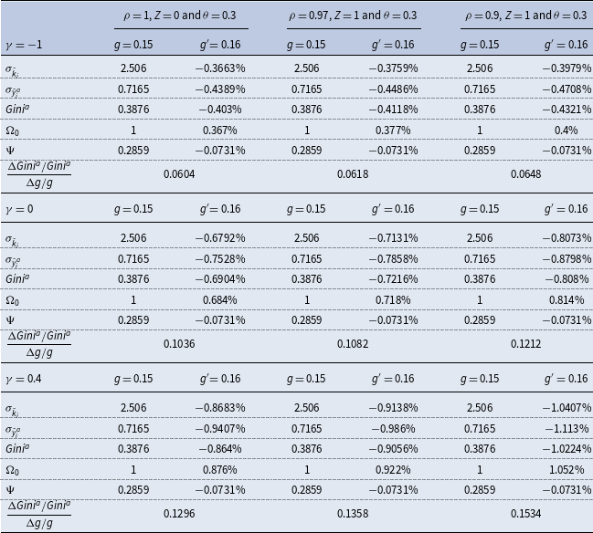
Table 4 also shows that when $\gamma =-1$
, the percentage reductions in the steady-state standard deviations of relative capital stock and posttax income, as well as the Gini coefficient, are all smaller (in absolute terms) under
$\gamma =-1$
, the percentage reductions in the steady-state standard deviations of relative capital stock and posttax income, as well as the Gini coefficient, are all smaller (in absolute terms) under $\theta =0.3$
than those corresponding to Table 2 with
$\theta =0.3$
than those corresponding to Table 2 with $\theta =0$
. In this environment with
$\theta =0$
. In this environment with $C_{t}$
and
$C_{t}$
and $G_{t}$
as Edgeworth substitutes, a higher
$G_{t}$
as Edgeworth substitutes, a higher $g$
leads to decreases in the marginal utilities of private consumption and leisure, which in turn induces each agent to work harder along the transition path such that the long-run distribution of individual hours worked will become less unequal. Using equations (38) and (39), it can be derived that there exists a negative correlation between the dispersion of labor supply and that of wealth/capitalFootnote 17 because relatively poor (wealthy) households choose to accumulate their capital more rapidly (slowly) during the transition. Consequently, the resulting wealth/capital inequality effect is weakened upon an increase in the government size. The same intuitive explanation is applicable to the setting with
$g$
leads to decreases in the marginal utilities of private consumption and leisure, which in turn induces each agent to work harder along the transition path such that the long-run distribution of individual hours worked will become less unequal. Using equations (38) and (39), it can be derived that there exists a negative correlation between the dispersion of labor supply and that of wealth/capitalFootnote 17 because relatively poor (wealthy) households choose to accumulate their capital more rapidly (slowly) during the transition. Consequently, the resulting wealth/capital inequality effect is weakened upon an increase in the government size. The same intuitive explanation is applicable to the setting with $\gamma =0.4$
, as the stationary-state standard deviation of labor hours will decline as well when private consumption and public good are preference complements. Thanks to a weaker wealth/capital inequality effect, the calculated elasticities of
$\gamma =0.4$
, as the stationary-state standard deviation of labor hours will decline as well when private consumption and public good are preference complements. Thanks to a weaker wealth/capital inequality effect, the calculated elasticities of $Gini^{a}$
with respect to public spending under either nonseparable specification of utility-generating government expenditure (
$Gini^{a}$
with respect to public spending under either nonseparable specification of utility-generating government expenditure ( $\gamma \neq 0$
), as shown in the top and bottom portions of Table 4, are lower than those in Table 2 for the benchmark model. It follows that these numerical elasticity results are not empirically plausible compared to recent estimates found by Doerrenberg and Peichl (Reference Doerrenberg and Peichl2014) and Guzi and Kahanec (Reference Guzi and Kahanec2018). Overall, this paper shows that under (i) a mild level of productive public-expenditure externalities (
$\gamma \neq 0$
), as shown in the top and bottom portions of Table 4, are lower than those in Table 2 for the benchmark model. It follows that these numerical elasticity results are not empirically plausible compared to recent estimates found by Doerrenberg and Peichl (Reference Doerrenberg and Peichl2014) and Guzi and Kahanec (Reference Guzi and Kahanec2018). Overall, this paper shows that under (i) a mild level of productive public-expenditure externalities ( $\chi =0.1$
) and (ii) a sufficiently high intertemporal elasticity of consumption substitution (
$\chi =0.1$
) and (ii) a sufficiently high intertemporal elasticity of consumption substitution ( $\gamma \geq 0$
), our calibrated monopolistically competitive Ramsey model is able to generate qualitatively as well as quantitatively realistic net-income-inequality effects of government spending vis-à-vis previous econometric studies.
$\gamma \geq 0$
), our calibrated monopolistically competitive Ramsey model is able to generate qualitatively as well as quantitatively realistic net-income-inequality effects of government spending vis-à-vis previous econometric studies.
5. Conclusion
Recent empirical studies have documented that there exists a discernible negative correlation between aggregate public expenditures and net-income inequality and that the estimated calculated elasticities of after-tax Gini with respect to government size range over the interval $[0.22$
,
$[0.22$
, $0.38]$
. Motivated by these stylized facts, this paper examines the distributional impact of government spending on agents’ disposable income, not only theoretically but also quantitatively, in a tractable monopolistically competitive Ramsey model with heterogeneous households and free entry/exit of intermediate goods-producing firms. We analytically show that upon an increase in the GDP fraction of government purchases, whether the long-run distribution of disposable income becomes more or less unequal is governed by the direction and size of the (unambiguously negative) wealth/capital inequality effect versus those of the (positive or negative) adjusted-labor effect. In a calibrated version of the model economy, our baseline setting correctly yields that a higher wasteful public-spending share will decrease the steady-state dispersion of posttax income, but the resulting calculated elasticities as shown in Tables 1 and 2 are too low to be empirically realistic. In light of these numerical findings, an otherwise identical monopolistically competitive Ramsey macroeconomy with useful government purchases of final goods and services is analyzed. We find that under (i) a mild level of productive public-spending externalities and (ii) a sufficiently high IES in consumption, our augmented model is able to generate qualitatively as well as quantitatively consistent net-income-inequality effects of government expenditures vis-à-vis the estimation results reported by Doerrenberg and Peichl (Reference Doerrenberg and Peichl2014) and Guzi and Kahanec (Reference Guzi and Kahanec2018).
$0.38]$
. Motivated by these stylized facts, this paper examines the distributional impact of government spending on agents’ disposable income, not only theoretically but also quantitatively, in a tractable monopolistically competitive Ramsey model with heterogeneous households and free entry/exit of intermediate goods-producing firms. We analytically show that upon an increase in the GDP fraction of government purchases, whether the long-run distribution of disposable income becomes more or less unequal is governed by the direction and size of the (unambiguously negative) wealth/capital inequality effect versus those of the (positive or negative) adjusted-labor effect. In a calibrated version of the model economy, our baseline setting correctly yields that a higher wasteful public-spending share will decrease the steady-state dispersion of posttax income, but the resulting calculated elasticities as shown in Tables 1 and 2 are too low to be empirically realistic. In light of these numerical findings, an otherwise identical monopolistically competitive Ramsey macroeconomy with useful government purchases of final goods and services is analyzed. We find that under (i) a mild level of productive public-spending externalities and (ii) a sufficiently high IES in consumption, our augmented model is able to generate qualitatively as well as quantitatively consistent net-income-inequality effects of government expenditures vis-à-vis the estimation results reported by Doerrenberg and Peichl (Reference Doerrenberg and Peichl2014) and Guzi and Kahanec (Reference Guzi and Kahanec2018).
Our analysis can be extended in several directions. In particular, it would be worthwhile to incorporate specific categories of government expenditures that have been found to exert statistically significant effects on income inequality into our Ramsey model, such as social security and public spending on welfare, education, and public health, among others. Moreover, while this paper focuses exclusively on the spending side of government budget, it would also be valuable to examine the distributional consequences of distortionary (capital or labor) income taxation. These possible extensions will enhance our understanding of how distinct types of government purchases and/or different fiscal policy rules affect income inequality within a monopolistic competitive macroeconomy. We plan to pursue these research projects in the near future.
Acknowledgements
We thank Stephen Turnovsky (Co-Editor), an anonymous referee, Been-Lon Chen, Yi-Ting Chen, YiLi Chien, Miroslav Gabrovski, Sharon Harrison, and Victor Ortego-Marti for helpful comments and discussions. Financial support provided by the Academia Sinica Investigator Award and the Ministry of Science and Technology, R.O.C., is gratefully acknowledged by Chang. Part of this research was conducted while Guo was a visiting research fellow of economics at Academia Sinica, Taipei, Taiwan, whose hospitality is greatly appreciated. Of course, all remaining errors are our own.
Appendix A
It can be shown that the elements which make up the benchmark model’s Jacobian matrix $\mathbf{J}$
as shown in (32) are as follows:
$\mathbf{J}$
as shown in (32) are as follows:
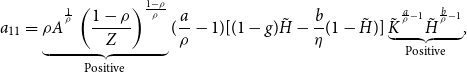 \begin{align} a_{11}& =\underbrace{\rho A^{^{\frac{1}{\rho }}}\left ( \frac{1-\rho }{Z}\right ) ^{\frac{1-\rho }{\rho }}}_{\textrm{Positive}}(\frac{a}{\rho }-1)[(1-g)\tilde{H}-\frac{b}{\eta }(1-\tilde{H})]\underbrace{\tilde{K}^{^{\frac{a}{\rho }-1}}\tilde{H}^{^{\frac{b}{\rho }-1}}}_{\textrm{Positive}}, \end{align}
 \begin{align} a_{12}& =\underbrace{\rho bA^{^{\frac{1}{\rho }}}\left ( \frac{1-\rho }{Z}\right ) ^{\frac{1-\rho }{\rho }}}_{\textrm{Positive}}\left \{ \frac{1}{\rho }[(1-g)\tilde{H}-\frac{b}{\eta }(1-\tilde{H})]+\frac{1}{\eta }\right \} \underbrace{\tilde{K}^{^{\frac{a}{\rho }}}\tilde{H}^{^{\frac{b}{\rho }-2}}}_{\textrm{Positive}}, \end{align}
 \begin{align} a_{21}& =\frac{\rho aA^{^{\frac{1}{\rho }}}\left ( \frac{1-\rho }{Z}\right ) ^{\frac{1-\rho }{\rho }}(\frac{a}{\rho }-1)\left \{ \left [ \frac{(1-\gamma )(1-g)}{\rho }-1\right ] \tilde{H}-\frac{b(1-\gamma )}{\rho \eta }(1-\tilde{H})\right \} \tilde{K}^{^{\frac{a}{\rho }-2}}\tilde{H}^{^{\frac{b}{\rho }}}}{(1-\gamma )(1-\frac{b}{\rho })+[1-\gamma (1+\eta )]\left ( \frac{\tilde{H}}{1-\tilde{H}}\right ) }, \end{align}
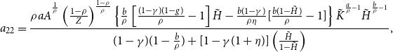 \begin{align} a_{22}& =\frac{\rho aA^{^{\frac{1}{\rho }}}\left ( \frac{1-\rho }{Z}\right ) ^{\frac{1-\rho }{\rho }}\left \{ \frac{b}{\rho }\left [ \frac{(1-\gamma )(1-g)}{\rho }-1\right ] \tilde{H}-\frac{b(1-\gamma )}{\rho \eta }[\frac{b(1-\tilde{H})}{\rho }-1]\right \} \tilde{K}^{^{\frac{a}{\rho }-1}}\tilde{H}^{^{\frac{b}{\rho }-1}}}{(1-\gamma )(1-\frac{b}{\rho })+[1-\gamma (1+\eta )]\left ( \frac{\tilde{H}}{1-\tilde{H}}\right ) }, \end{align}
where $\tilde{H}$
and
$\tilde{H}$
and $\tilde{K}$
are given by (28) and (29), respectively.
$\tilde{K}$
are given by (28) and (29), respectively.
Using the steady-state version of the aggregate capital accumulation equation (26) with $\dot{K}_{t}=0$
, it is straightforward to show that
$\dot{K}_{t}=0$
, it is straightforward to show that
 \begin{equation} (1-g)\tilde{H}-\frac{b}{\eta }(1-\tilde{H})=\frac{\delta }{\rho A^{^{\frac{1}{\rho }}}\left ( \frac{1-\rho }{Z}\right ) ^{\frac{1-\rho }{\rho }}\tilde{K}^{^{\frac{a}{\rho }-1}}\tilde{H}^{^{\frac{b}{\rho }-1}}}\gt 0, \end{equation}
which, combined with $\frac{a}{\rho }\lt 1$
to rule out sustained long-run economic growth, leads to
$\frac{a}{\rho }\lt 1$
to rule out sustained long-run economic growth, leads to $a_{11}\lt 0$
. In addition, condition (A5) together with
$a_{11}\lt 0$
. In addition, condition (A5) together with $\eta \gt 0$
and
$\eta \gt 0$
and $\rho \in (0,$ $1)$
imply that
$1)$
imply that $a_{12}\gt 0$
.
$a_{12}\gt 0$
. $\blacksquare$


