


1 Introduction
While machine learning (ML) systems have revolutionized many aspects of human lives, the growing evidence of algorithmic bias necessitates the need for fairness-aware ML. ML algorithms rely on the training data to make predictions that often have high societal impacts, such as determining the likelihood of convicted criminals re-offending (Dressel & Farid, Reference Dressel and Farid2018). Thus, algorithms that are trained on a biased representation of the actual population could disproportionately disadvantage a specific group or groups. Although most examples of algorithmic bias in ML occur due to the training data, recent work shows that the algorithm itself can introduce bias or amplify existing bias (Kamishima et al., Reference Kamishima, Akaho, Asoh and Sakuma2012; Baeza-Yates, Reference Baeza-Yates2018; Cunningham & Delany, Reference Cunningham, Delany, Heintz, Milano and O’Sullivan2020; Hooker et al., Reference Hooker, Moorosi, Clark, Bengio and Denton2020; Blanzeisky & Cunningham, Reference Blanzeisky and Cunningham2021). When the bias occurs due to the data, it is sometimes euphemistically called negative legacy; it is called underestimation when it is due to the algorithm (Kamishima et al., Reference Kamishima, Akaho, Asoh and Sakuma2012; Cunningham & Delany, Reference Cunningham, Delany, Heintz, Milano and O’Sullivan2020).
Over the past few years, several approaches to mitigate bias in ML have been proposed (Caton & Haas, Reference Caton and Haas2020). One strategy is to modify an algorithm’s objective function to account for one or more fairness measures. For example, one can enforce a fairness measure as a constraint directly into the algorithm’s optimization function (Zemel et al., Reference Zemel, Wu, Swersky, Pitassi, Dwork, Dasgupta and McAllester2013). From this perspective, algorithmic bias can be formulated as a multi-objective optimization problem (MOOP), where the objective is usually to maintain good predictive accuracy while ensuring fair outcomes across sensitive groups. The main challenge with these approaches is that they usually result in a non-convex optimization function (Goel et al., Reference Goel, Yaghini and Faltings2018). Although convexity is often required for algorithmic convenience, there are several possible approaches to address this issue; Zafar et al. (Reference Zafar, Valera, Rodriguez and Gummadi2015) use the co-variance between sensitive attribute and target feature as a proxy for a convex approximate measure of fairness, Zafar et al. (Reference Zafar, Valera, Gomez Rodriguez and Gummadi2017) convert non-convex fairness constraint into a Disciplined Convex-Concave Program (DCCP) and leverage recent advances in convex-concave programming to solve it, while Cotter et al. (Reference Cotter, Friedlander, Goh and Gupta2016) utilizes majorization-minimization procedure for (approximately) optimizing non-convex function.
In this paper, we focus on mitigating underestimation bias. Specifically, we formulate underestimation as a MOOP and propose a remediation strategy using Pareto Simulated Annealing (PSA) to simultaneously optimize the algorithm on two objectives: (1) maximizing prediction accuracy; (2) ensuring little to no underestimation bias. Since the optimization in MOOP is usually a compromise between multiple competing solutions (in our case, accuracy and underestimation), the main objective is to use Pareto optimality to find a set of optimal solutions created by the two competing criteria (Mas-Colell et al., Reference Mas-Colell, Whinston and Green1995).
The specifics of the proposed remediation strategy are presented in more detail in Section 4. Before that, the relevant background on key concepts used in this paper is reviewed in Sections 2 and 3. The paper concludes in Section 5 with an assessment of how this repair strategy works on two synthetic and two real datasets.
2 Bias in machine learning
Existing research in ML bias can generally be categorized into two groups: bias discovery and bias mitigation (Zliobaite, Reference Zliobaite2017). Most literature on bias discovery focuses on quantifying bias and developing a theoretical understanding of the social and legal aspects of ML bias, while bias prevention focuses on technical approaches to mitigate biases in ML systems. Several notions to quantify fairness have been proposed (Caton & Haas, Reference Caton and Haas2020). One of the accepted measure of unfairness is Disparate Impact (DIs) (Feldman et al., Reference Feldman, Friedler, Moeller, Scheidegger and Venkatasubramanian2015):
 \begin{equation} \mathrm{DI}_S \leftarrow \frac{P[\hat{Y}= 1 | S = 0]}{P[\hat{Y} = 1 \vert S = 1]}
< \tau\end{equation}
\begin{equation} \mathrm{DI}_S \leftarrow \frac{P[\hat{Y}= 1 | S = 0]}{P[\hat{Y} = 1 \vert S = 1]}
< \tau\end{equation}
 $\mathrm{DI}_S$
is defined as the ratio of desirable outcomes
$\mathrm{DI}_S$
is defined as the ratio of desirable outcomes
 $\hat{Y}$
predicted for the protected group
$\hat{Y}$
predicted for the protected group
 $S = 0$
compared with that for the majority
$S = 0$
compared with that for the majority
 $S = 1$
.
$S = 1$
.
 $\tau = 0.8$
is the 80% rule, that is the proportion of desirable outcomes for the minority should be within 80% of those for the majority. However, this measure emphasizes fairness for the protected group without explicitly taking into account the source of the bias.
$\tau = 0.8$
is the 80% rule, that is the proportion of desirable outcomes for the minority should be within 80% of those for the majority. However, this measure emphasizes fairness for the protected group without explicitly taking into account the source of the bias.
As stated in Section 1, it is worth emphasizing the difference between negative legacy and underestimation as sources of bias in ML. Negative legacy refers to problems with the data while underestimation refers to the bias due to the algorithm. Negative legacy may be due to labeling errors or poor sampling; however, it is likely to reflect discriminatory practices in the past. On the other hand, underestimation occurs when the algorithm focuses on strong signals in the data thereby missing more subtle phenomena (Cunningham & Delany, Reference Cunningham, Delany, Heintz, Milano and O’Sullivan2020). Recent work shows that underestimation occurs when an algorithm underfits the training data due to a combination of limitations in training data and model capacity issues (Kamishima et al., Reference Kamishima, Akaho, Asoh and Sakuma2012; Cunningham & Delany, Reference Cunningham, Delany, Heintz, Milano and O’Sullivan2020; Blanzeisky & Cunningham, Reference Blanzeisky and Cunningham2021). It has also been shown that irreducible error, regularization and feature and class imbalance can contribute to this underestimation (Blanzeisky & Cunningham, Reference Blanzeisky and Cunningham2021).
If a classifier is unbiased in algorithmic terms at the class level, the proportion of a class in the predictions should be roughly the same as the proportion in the observations. It is well known that class imbalance in the training data can be accentuated in predictions (Japkowicz & Stephen, Reference Japkowicz and Stephen2002). This can be quantified using an underestimation score (US) as follows:
 \begin{equation} \mathrm{US} = \frac{P[\hat{Y} = 1]} { P[Y = 1]}\end{equation}
A US score significantly less than 1 would indicate that a classifier is under-predicting the Y = 1 class. This US score does not consider what is happening for protected or unprotected groups. For this we define
 $\mathrm{US}_{S=0}$
in line with
$\mathrm{US}_{S=0}$
in line with
 $\mathrm{DI}_S$
:
$\mathrm{DI}_S$
:
 \begin{equation} \mathrm{US}_{S=0} \leftarrow \frac{P[\hat{Y}= 1 | S = 0]}{P[Y = 1 | S = 0]}\end{equation}
This is the ratio of desirable outcomes predicted by the classifier for the protected group compared with what is actually present in the data (Cunningham & Delany, Reference Cunningham, Delany, Heintz, Milano and O’Sullivan2020). If
 $\mathrm{US}_{S=0} <1$
the classifier is under-predicting desirable outcomes for the minority. It is worth nothing that
$\mathrm{US}_{S=0} <1$
the classifier is under-predicting desirable outcomes for the minority. It is worth nothing that
 $\mathrm{US}_{S=0} = 1$
does not necessarily mean that the classifier is not biased against the minority group (i.e. poor
$\mathrm{US}_{S=0} = 1$
does not necessarily mean that the classifier is not biased against the minority group (i.e. poor
 $\mathrm{DI}_S$
score).
$\mathrm{DI}_S$
score).
An alternative underestimation score used by Kamishima et al. (Reference Kamishima, Akaho, Asoh and Sakuma2012) that considers divergences between overall actual and predicted distributions for all groups S is the underestimation index (UEI) based on the Hellinger distance:
 \begin{equation} \mathrm{UEI} = \sqrt{1-\sum_{y,s\in D} \sqrt{P[\hat{Y}=y,S=s]\times P[Y=y,S=s]}}\end{equation}
Here y and s are the possible values of Y and S respectively. This Hellinger distance is preferred to KL-divergence because it is bounded in the range [0,1] and KL-divergence has the potential to be infinite.
 $\mathrm{UEI} = 0$
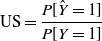
indicates that there is no difference between the probability distribution of the training samples and prediction made by a classifier (no underestimation). Although this notion is useful when quantifying the extent to which a model’s prediction deviates from the training samples, it does not directly tell us how the protected group is doing. This phenomenon is clearly illustrated in Figure 1.
$\mathrm{UEI} = 0$
indicates that there is no difference between the probability distribution of the training samples and prediction made by a classifier (no underestimation). Although this notion is useful when quantifying the extent to which a model’s prediction deviates from the training samples, it does not directly tell us how the protected group is doing. This phenomenon is clearly illustrated in Figure 1.
Figure 1. A comparison on the two underestimation measures UEI and US
 $_{\textrm{S}}$
on the four datasets summarized in Table 1. The UEI score is an aggregate score across all feature/outcomes and as such can hide detail of the impact on the protected group (S=0). This is evident when we compare the Recidivism and Adult scores.
$_{\textrm{S}}$
on the four datasets summarized in Table 1. The UEI score is an aggregate score across all feature/outcomes and as such can hide detail of the impact on the protected group (S=0). This is evident when we compare the Recidivism and Adult scores.
Figure 1 shows the UEI and US scores for the protected (
 $\mathrm{US}_{S = 0}$
) and unprotected groups (
$\mathrm{US}_{S = 0}$
) and unprotected groups (
 $\mathrm{US}_{S = 1}$
), and the overall underestimation score at a class level (US) of predictions made by logistic regression classifier on the four datasets introduced in Section 5. If our particular concern is the unprotected group it is clear that underestimation is not consistently captured by UEI. For instance, the UEI scores for the Adult and Recidivism datasets are similar at 0.09 and 0.08 respectively but the outcomes for the minority (
$\mathrm{US}_{S = 1}$
), and the overall underestimation score at a class level (US) of predictions made by logistic regression classifier on the four datasets introduced in Section 5. If our particular concern is the unprotected group it is clear that underestimation is not consistently captured by UEI. For instance, the UEI scores for the Adult and Recidivism datasets are similar at 0.09 and 0.08 respectively but the outcomes for the minority (
 $\mathrm{US}_{S = 0}$
) are very different (Adult: 0.28, Recidivism: 0.65). Because UEI considers all feature/class combinations it can sometimes obscure how the protected group is faring. Nevertheless, if our algorithmic objective is to ensure that distributions in predictions align with distributions in the training data UEI is an appropriate metric. The lesson from Figure 1 is that we should also consider US scores to really understand what is going on.
$\mathrm{US}_{S = 0}$
) are very different (Adult: 0.28, Recidivism: 0.65). Because UEI considers all feature/class combinations it can sometimes obscure how the protected group is faring. Nevertheless, if our algorithmic objective is to ensure that distributions in predictions align with distributions in the training data UEI is an appropriate metric. The lesson from Figure 1 is that we should also consider US scores to really understand what is going on.
A further lesson from Figure 1 is that underestimation for the minority group
 $\mathrm{US}_{S = 0}$
can differ significantly from the overall underestimation due to class imbalance (US). For all four datasets
$\mathrm{US}_{S = 0}$
can differ significantly from the overall underestimation due to class imbalance (US). For all four datasets
 $\mathrm{US}_{S = 0} <$
US; for the Adult dataset the difference is particularly evident. So when we have algorithmic bias due to class imbalance, the effect can be exacerbated for minority groups.
$\mathrm{US}_{S = 0} <$
US; for the Adult dataset the difference is particularly evident. So when we have algorithmic bias due to class imbalance, the effect can be exacerbated for minority groups.
2.1 Relationship between underestimation and accuracy
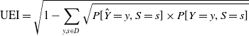
In this section, we examine the relationship between underestimation and accuracy. A trade-off between accuracy and fairness is almost taken as a given in the existing literature on fairness in machine learning (Dutta et al., Reference Dutta, Wei, Yueksel, Chen, Liu and Varshney2020). To further support this finding, we investigate the search space explored by our framework on a synthetic dataset. It is clear from Figure 2 that underestimation and accuracy is indeed orthogonal of each other. A Pearson correlation coefficient of –0.995 indicates a strong negative relationship between underestimation and accuracy. In addition, the conflicting nature of accuracy and underestimation (UEI) is also confirmed by the Pareto front in Figure 3. Hence, the problem of underestimation bias can be formulated as a multi-objective optimization problem where the two competing objectives are accuracy and underestimation. In the next section, we provide background information on multi-objective optimization.

Figure 2. Relationship between underestimation index (UEI) and accuracy.
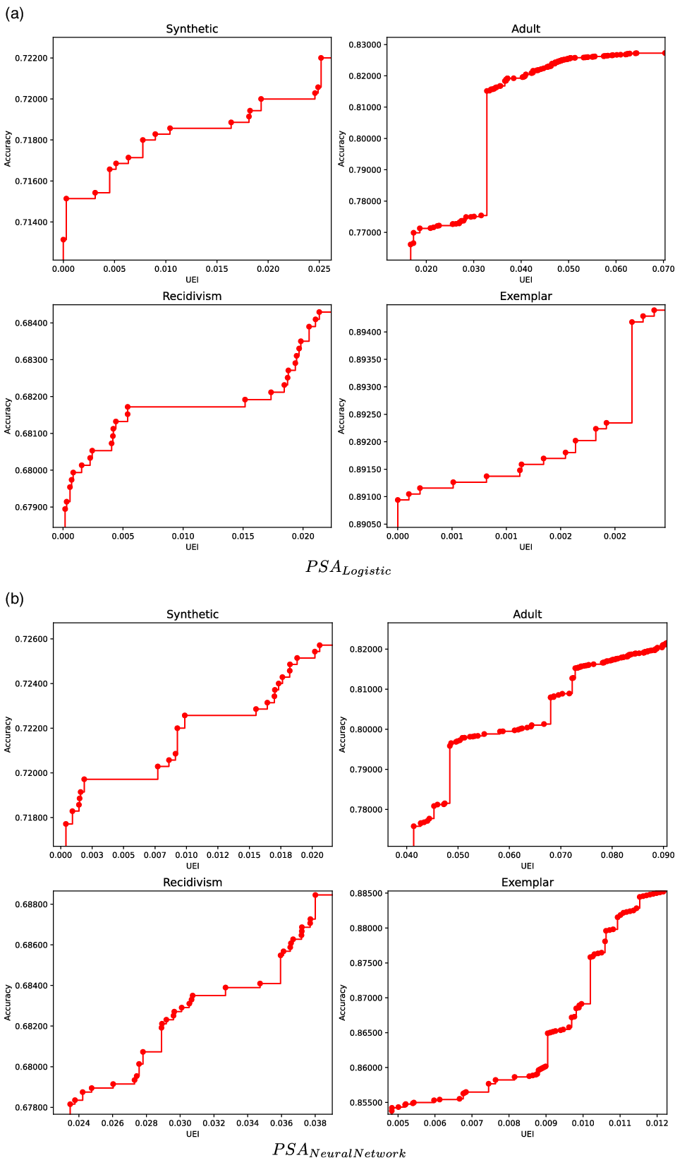
Figure 3. Pareto fronts obtained using Pareto Simulated Annealing on four datasets.
3 Multi-objective optimization
Multi-objective optimization problems (MOOPs) are problems where two or more objective functions have to be simultaneously optimized. Given two or more objective functions
 $c_{i}$
for
$c_{i}$
for
 $i = 1,2,...,m$
, MOOP can generally be formulated as:
$i = 1,2,...,m$
, MOOP can generally be formulated as:
 \begin{equation} \min_x (c_{1}(x),c_{2}(x),c_{3}(x),...,c_{m}(x))\end{equation}
As stated in Section 1, ensuring fairness while optimizing for accuracy in ML algorithms can be formulated as an MOOP. If the objective is to produce fair classifiers then there are two objective functions, accuracy and UEI. We have seen in Section 2.1 that these criteria are in conflict so we can expect scenarios where no improvement in one objective is possible without making things worse in the other. When there is no single solution that dominates in both criteria, the concept of Pareto optimality is used to find a set of non-dominated solutions created by the two competing criteria (Mas-Colell et al., Reference Mas-Colell, Whinston and Green1995). This set of solutions is also referred to as the Pareto set; example Pareto sets are shown in Figure 3. Pareto optimization cannot be computed efficiently in many cases as they are often of exponential size. Thus, approximation methods for them are frequently used. Various methods to solve MOOP have been proposed (Deb, Reference Deb2014). One strategy is to use meta-heuristics to solve multi-objective combinatorial optimization problems. A comprehensive study on multi-objective optimization by meta-heuristics can be found in Jaszkiewicz (Reference Jaszkiewicz2001). These algorithms are usually based on employing evolutionary optimization algorithms due to its gradient-free mechanism and the local optima avoidance.
3.1 Simulated annealing
Simulated annealing (SA) is a single-objective meta-heuristic to approximate a global optimization function with a very large search space (Kirkpatrick et al., Reference Kirkpatrick, Gelatt and Vecchi1983). SA is similar to stochastic hill-climbing but with provision to allow for worse solutions to be accepted with some probability (Foley et al., Reference Foley, Greene and Cunningham2010). Inspired by the natural process of annealing solids in metallurgy, the acceptance of inferiors solutions is controlled by a temperature variable T so that it will becomes increasingly unlikely as the system cools down. This will allow SA to escape from local minima, which is often desirable when optimizing non-convex functions.
Given an objective function c(x), initial solution x, and initial temperature T, the simulated annealing process consists of first finding a neighbor
 $\bar{x}$
as a candidate solution by perturbing the initial solution x. If the candidate solution
$\bar{x}$
as a candidate solution by perturbing the initial solution x. If the candidate solution
 $\bar{x}$
improves on x, then it is accepted with a probability of 1. In contrast, if
$\bar{x}$
improves on x, then it is accepted with a probability of 1. In contrast, if
 $\bar{x}$
is worse than x, it may still be accepted with a probability
$\bar{x}$
is worse than x, it may still be accepted with a probability
 $P(x,\bar{x},T)$
. The acceptance probability for inferior solutions follows a Boltzmann probability distribution and can be defined as (Czyzżak & Jaszkiewicz, Reference Czyzżak and Jaszkiewicz1998):
$P(x,\bar{x},T)$
. The acceptance probability for inferior solutions follows a Boltzmann probability distribution and can be defined as (Czyzżak & Jaszkiewicz, Reference Czyzżak and Jaszkiewicz1998):
 \begin{equation} P(x,\bar{x},T) = \min \left( 1,exp\left(\frac{c(x) - c(\bar{x})}{T}\right) \right)\end{equation}
This stochastic search process is repeated
 $n_{iter}$
times for each temperature T, while the decrease in T is controlled by a cooling rate
$n_{iter}$
times for each temperature T, while the decrease in T is controlled by a cooling rate
 $\alpha$
. The process stops once changes stop being accepted.
$\alpha$
. The process stops once changes stop being accepted.
3.2 Pareto simulated annealing
Pareto Simulated Annealing (PSA) is an extension of SA for handling MOOP by exploiting the idea of constructing an estimated Pareto set (Amine, Reference Amine2019). Instead of starting with one solution, PSA initializes a set of solutions. Candidate solutions are generated from this set to obtain a diversified Pareto front. PSA aggregates the acceptance probability for all the competing criteria so that the acceptance probability of inferior solutions is defined as (Czyzżak & Jaszkiewicz, Reference Czyzżak and Jaszkiewicz1998):
 \begin{equation} P(x,\bar{x},T,\lambda) = \min \left \{ 1,exp\left(\frac{\sum_{i=0}^{m} \lambda_{i} (c_{i}(x) - c_{i}(\bar{x}))}{T}\right) \right\}\end{equation}
where m is the number of objectives to be optimized and
 $\lambda$
is a weight vector that represents the varying magnitude of importance of the objectives. Depending on the units of the criteria, it may be desirable to normalize the function so that the movement of a function in one solution when compared with the function in the original solution are treated as percentage improvements (Foley et al., Reference Foley, Greene and Cunningham2010). In other words, the differences in particular objectives for acceptance criteria probability calculation are aggregated with a simple weighted sum. It is worth noting that the temperature T is dependent on the range of the objective functions.
$\lambda$
is a weight vector that represents the varying magnitude of importance of the objectives. Depending on the units of the criteria, it may be desirable to normalize the function so that the movement of a function in one solution when compared with the function in the original solution are treated as percentage improvements (Foley et al., Reference Foley, Greene and Cunningham2010). In other words, the differences in particular objectives for acceptance criteria probability calculation are aggregated with a simple weighted sum. It is worth noting that the temperature T is dependent on the range of the objective functions.
PSA has shown significant success for many applications; designing optimal water distribution networks (Cunha & Marques, Reference Cunha and Marques2020), optimizing control cabinet layout (Pllana et al., Reference Pllana, Memeti and Kolodziej2019), optimizing for accuracy and sparseness in non-negative matrix factorization (Foley et al., Reference Foley, Greene and Cunningham2010), etc. Furthermore, there are several variants of PSA in the literature. Implementation details of these variants can be found in (Amine, Reference Amine2019).
4 Training for accuracy and underestimation
Given a dataset D(X, Y), the goal of supervised ML is to learn an input-output mapping function
 $f\,{:}\, X\,{\rightarrow}\,Y$
that will generalize well on unseen data. From the optimization perspective, the learning process can be viewed as finding the mapping that performs best in terms of how good the prediction model f(X) does with regard to the expected outcome Y. For example, logistic regression, a well-studied algorithm for classification, can be formulated as an optimization problem where the objective is to learn the best mapping of feature vector X to the target feature Y through a probability distribution:
$f\,{:}\, X\,{\rightarrow}\,Y$
that will generalize well on unseen data. From the optimization perspective, the learning process can be viewed as finding the mapping that performs best in terms of how good the prediction model f(X) does with regard to the expected outcome Y. For example, logistic regression, a well-studied algorithm for classification, can be formulated as an optimization problem where the objective is to learn the best mapping of feature vector X to the target feature Y through a probability distribution:
 \begin{equation} P(Y = 1|X,\theta) = \frac{1}{1+e^{- \theta^T \cdot X}}\end{equation}
where
 $\theta$
, the regression coefficients are obtained by solving an optimization problem to minimize log loss
$\theta$
, the regression coefficients are obtained by solving an optimization problem to minimize log loss
 $L_{\theta}$
:
$L_{\theta}$
:
 \begin{equation} L_{\theta} = -y \cdot log(P(Y = 1|X,\theta)) + (1-y) \cdot log(1-P(Y = 1|X,\theta))\end{equation}
Solving this optimization problem directly without any explicit consideration of fairness could result in a model in which predictions show significant bias against a particular social group. To address this issue, one could directly modify the loss function in 9 by adding a fairness constraint, see for example Zafar et al. (Reference Zafar, Valera, Rodriguez and Gummadi2015). The optimization is typically performed using variants of stochastic gradient descent (SGD). However, directly incorporating a fairness constraint into the loss function often results in a non-convex loss function. Consequently, optimizers that rely on the gradient of the loss function will struggle to converge due to the fact that non-convex functions have potentially many local minima (or maxima) and saddle points. Furthermore, many single objective optimization problems are NP-hard, and thus it is reasonable to expect that generating efficient solutions for MOOP is not easy (Czyzżak & Jaszkiewicz, Reference Czyzżak and Jaszkiewicz1998). Due to this complexity, we propose a multi-objective optimization strategy using PSA to optimize for accuracy and underestimation.
To illustrate the effectiveness of PSA to mitigate underestimation, we implement PSA for logistic regression and neural networks. The aim is to find a set of
 $\theta$
parameters that gives the highest accuracy and lowest UEI. The details of the model are described in the next subsection (see Section 4.1). Given a dataset
$\theta$
parameters that gives the highest accuracy and lowest UEI. The details of the model are described in the next subsection (see Section 4.1). Given a dataset
 $\mathcal{D}(X,Y,S)$
, where X represents the feature vector, target label Y and sensitive attribute S, let
$\mathcal{D}(X,Y,S)$
, where X represents the feature vector, target label Y and sensitive attribute S, let
 $\hat{Y}$
be the prediction output of a model
$\hat{Y}$
be the prediction output of a model
 $\mathcal{M}(\theta,X,S)$
. The optimization problem can be formally defined as:
$\mathcal{M}(\theta,X,S)$
. The optimization problem can be formally defined as:
 \begin{equation} \theta = arg\max_\theta \left( Acc(Y,\hat{Y}),\frac{1}{UEI(Y,\hat{Y},S)} \right)\end{equation}
where
 $Acc(Y,\hat{Y})$
represents the accuracy of classification prediction:
$Acc(Y,\hat{Y})$
represents the accuracy of classification prediction:
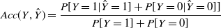 \begin{equation} Acc(Y,\hat{Y}) = \frac{P[Y=1|\hat{Y}=1] + P[Y= 0|\hat{Y}= 0]]}{P[Y=1] + P[Y = 0]}\end{equation}
The high-level description of our framework is presented in Algorithm 1. The exact implementation can be found on Github.Footnote 1 Our algorithm is a modification of the PSA algorithm in (Czyzżak & Jaszkiewicz, Reference Czyzżak and Jaszkiewicz1998) tailored to optimize for accuracy and UEI. It is worth noting that the choice of an appropriate cooling rate and initial temperature is crucial in order to ensure success of the algorithm (Amine, Reference Amine2019).

Algorithm 1: High-level pseudocode for Pareto Simulated Annealing algorithm to mitigate underestimation.
Given an initial temperatures T, perturbation scale
 $\beta$
and cooling rate
$\beta$
and cooling rate
 $\alpha$
, the PSA process consists of two loops (See line 5 and 6 in Algorithm 1); the first loop begins by randomly creating a set of solutions
$\alpha$
, the PSA process consists of two loops (See line 5 and 6 in Algorithm 1); the first loop begins by randomly creating a set of solutions
 $Set_{\theta}$
with each solution representing a current solution
$Set_{\theta}$
with each solution representing a current solution
 $\theta$
. Then, for each
$\theta$
. Then, for each
 $\theta$
in
$\theta$
in
 $Set_{\theta}$
, a candidate solution
$Set_{\theta}$
, a candidate solution
 $\bar{\theta}$
is created by perturbing one of its dimensions with Gaussian noise
$\bar{\theta}$
is created by perturbing one of its dimensions with Gaussian noise
 $X \sim \mathcal{N}(0,\beta^2)$
. The candidate solution is accepted as the current best solution if it is better than the initial solution. If the candidate solution is dominated by the current best solution, it will only be accepted if
$X \sim \mathcal{N}(0,\beta^2)$
. The candidate solution is accepted as the current best solution if it is better than the initial solution. If the candidate solution is dominated by the current best solution, it will only be accepted if
 $P(\theta,\bar{\theta},T)$
is larger than a random value sampled from a uniform distribution
$P(\theta,\bar{\theta},T)$
is larger than a random value sampled from a uniform distribution
 $\mathcal{U}(0,1)$
. Since the objective is to find the best solution
$\mathcal{U}(0,1)$
. Since the objective is to find the best solution
 $\theta$
that gives the best accuracy and UEI score, we set
$\theta$
that gives the best accuracy and UEI score, we set
 $\lambda$
to 1. This process is repeated for some iterations (see line 6). The second loop repeats this overall process (first loop) and iteratively decrease the temperature by a cooling rate
$\lambda$
to 1. This process is repeated for some iterations (see line 6). The second loop repeats this overall process (first loop) and iteratively decrease the temperature by a cooling rate
 $\alpha$
until no further changes to the best solution occur. The PSA algorithm will return a set of solutions
$\alpha$
until no further changes to the best solution occur. The PSA algorithm will return a set of solutions
 $Set_{Pareto}$
. We will then use the concept of Pareto optimality to select solutions that are non-dominated in terms of both criteria, referred to as the Pareto set (Amine, Reference Amine2019). A solution is said to be Pareto optimal if it is impossible to make one criterion better without making another criterion worse.
$Set_{Pareto}$
. We will then use the concept of Pareto optimality to select solutions that are non-dominated in terms of both criteria, referred to as the Pareto set (Amine, Reference Amine2019). A solution is said to be Pareto optimal if it is impossible to make one criterion better without making another criterion worse.
There are advantages and disadvantages to using PSA to mitigate underestimation. First, one could directly incorporate fairness constraints as the objective functions to be optimized without having to use a proxy convex function as an approximate measure of how good the predictions of a model is in terms of the expected outcome Y. Second, PSA is straightforward to implement and its characteristic of accepting inferior solutions allows escaping from local minima/maxima, which is often desirable when the search space is large and the optimization functions are not convex. However, one limitation of PSA is that its implementation is problem-dependent, and the choice of appropriate parameters is itself a challenging task. Thus, preliminary experiments are often required (Amine, Reference Amine2019).
4.1 Model details
We evaluated our framework on two classifiers: logistic regression and neural networks. In logistic regression, the solution
 $\theta$
is simply a vector of beta coefficients of size
$\theta$
is simply a vector of beta coefficients of size
 $m + 1$
, where m is the number of features in the training data and an additional intercept coefficient. For our neural network we consider an architecture that has five nodes in one hidden layer. Thus, the number of parameters to be estimated
$m + 1$
, where m is the number of features in the training data and an additional intercept coefficient. For our neural network we consider an architecture that has five nodes in one hidden layer. Thus, the number of parameters to be estimated
 $|\theta|$
is
$|\theta|$
is
 $ ((m + 1) \times 5) + 5$
. For instance, for the Exemplar dataset which has 18 features, the number of parameters in the neural network is
$ ((m + 1) \times 5) + 5$
. For instance, for the Exemplar dataset which has 18 features, the number of parameters in the neural network is
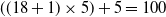 $((18 + 1) \times 5) + 5 = 100$
parameters.
$((18 + 1) \times 5) + 5 = 100$
parameters.
5 Experiments
In this section, we experimentally validate our framework described in Section 4 on four datasets. Evaluations on bias in ML are necessarily limited because of the availability of relevant datasets. Our evaluation considers the synthetic dataset introduced in Feldman et al. (Reference Feldman, Friedler, Moeller, Scheidegger and Venkatasubramanian2015), the synthetic exemplar dataset in Blanzeisky et al. (Reference Blanzeisky, Cunningham and Kennedy2021), the reduced version of the Adult dataset (Kohavi, Reference Kohavi1996) and the ProPublica Recidivism dataset (Dressel & Farid, Reference Dressel and Farid2018). These datasets have been extensively studied in fairness research because there is clear evidence of negative legacy. Summary statistics for these datasets are provided in Table 1.
Table 1. Summary details of the four datasets
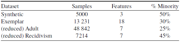
The prediction task for the Adult dataset is to determine whether a person earns more or less than
 $\$$
50 000 per year based on their demographic information. We remove all the other categorical features in the Adult dataset except the sensitive attribute Sex. The reduced and anonymized version of the Recidivism dataset includes seven features and the target variable is Recidivism. The goal of our experiment is to learn an underestimation-free classifier while maintaining a high accuracy score when Gender, Age, Sex and Caucasian as sensitive features S for the Synthetic, Exemplar, Adult and Recidivism datasets, respectively.
$\$$
50 000 per year based on their demographic information. We remove all the other categorical features in the Adult dataset except the sensitive attribute Sex. The reduced and anonymized version of the Recidivism dataset includes seven features and the target variable is Recidivism. The goal of our experiment is to learn an underestimation-free classifier while maintaining a high accuracy score when Gender, Age, Sex and Caucasian as sensitive features S for the Synthetic, Exemplar, Adult and Recidivism datasets, respectively.
5.1 Generating pareto fronts
To illustrate the effectiveness of the proposed strategy, we compare against classifiers optimized using Stochastic Gradient Descent (SGD) from scikit-learnFootnote 2 as baselines. Specifically, we tested our framework on two classifiers: logistic regression (
 $\mathrm{PSA}_{Logistic}$
) and neural networks (
$\mathrm{PSA}_{Logistic}$
) and neural networks (
 $\mathrm{PSA}_{NeuralNetwork}$
) and compare performance against the SGD variants of each classifier (
$\mathrm{PSA}_{NeuralNetwork}$
) and compare performance against the SGD variants of each classifier (
 $\mathrm{SGD}_{Logistic}$
,
$\mathrm{SGD}_{Logistic}$
,
 $\mathrm{SGD}_{NeuralNetwork}$
).
$\mathrm{SGD}_{NeuralNetwork}$
).
For each of the datasets we use a 70:30 train test split. Figure 3 shows the Pareto front obtained by
 $\mathrm{PSA}_{Logistic}$
and
$\mathrm{PSA}_{Logistic}$
and
 $\mathrm{PSA}_{NeuralNetwork}$
on the training sets. For this example, we set the parameters for the PSA algorithm 1 as follows:
$\mathrm{PSA}_{NeuralNetwork}$
on the training sets. For this example, we set the parameters for the PSA algorithm 1 as follows:
-
Initial temperature ( T ): 0.1. This parameter controls the exploration phase of PSA because it directly impacts the likelihood of accepting inferior solutions. It allows PSA to move freely about the search space with the hope that PSA finds a region with the best local minimum to exploit.
-
Perturbation scale (
 $\beta$
): 0.1. This parameter is relative to bounds of the search space. It allows PSA to generate a candidate solution where the mean is the initial solution and the standard deviation is defined by this parameter
$\beta$
.
$\beta$
): 0.1. This parameter is relative to bounds of the search space. It allows PSA to generate a candidate solution where the mean is the initial solution and the standard deviation is defined by this parameter
$\beta$
. -
Cooling rate (
$\alpha$
): 0.95. It controls the exploitation phase of the search process by reducing the stochasticity and forcing the search to converge to a minimum. Setting
$\alpha$
to 0.95 typically causes PSA to converge after
$\sim$
80 iterations (step 5 in Algorithm 1). -
Number of iterations (
$n_{iter}$
): 1000 successes or 10 000 attempts. For each temperature, PSA will repeat generating and evaluating candidate solutions until 1000 better solutions are found or 10 000 attempts have been made. -
Size of the initial solutions set (
$|Set_{\theta}|$
): 3. The value of this parameter will determine the quality of the Pareto front produced.


Finding a suitable and reasonable trade-off between exploration and exploitation is crucial for the success of PSA in mitigating underestimation. The main objective is to find the best set of parameters that will allow PSA to explore large enough search space while ensuring the algorithm converges to near-optimal solution within reasonable time. Our preliminary experiments suggest that the initial temperature T has to be set such that the likelihood of accepting worse solutions starts high at the beginning of the search and decreases with the progress of the search, giving the algorithm the opportunity to first locate the region for the global optima, escaping local optima, then iteratively progresses to the optima itself. With these parameters, a typical run will consider between 100 000 and 500 000 solutions. We can see from the Pareto fronts that the two criteria are in conflict. For logistic regression, for all but the Adult dataset, PSA finds models that eliminate underestimation (UEI = 0) on the training data. If we look closely at the x axes, we see that this is being achieved with a loss of 1% to 2% in classification accuracy. The neural network results are not quite so good, possibly because of the larger parameter space.
A close examination of the two Pareto fronts for the Adult dataset suggests that eliminating underestimation is more challenging for this task. No models are found that bring the UEI score to zero.
5.2 Assessing generalization performance
We turn now to considering the generalization performance of these models on the test data that has been held back. For all evaluations, the policy has been to select models with lowest UEI on the training data, these would be the models on the bottom left of the Parteo fronts. The accuracy and UEI scores for these models on the test data are shown in Figure 4 and accuracy and
 $\mathrm{US}_{S=0}$
scores are shown in Figure 5.
$\mathrm{US}_{S=0}$
scores are shown in Figure 5.
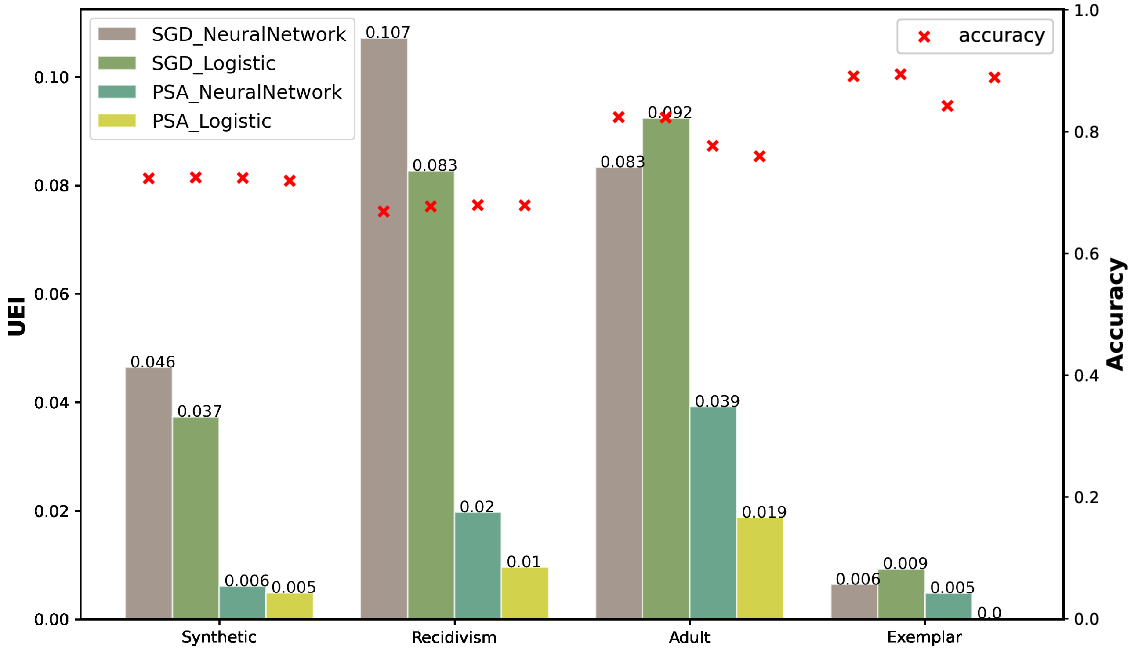
Figure 4. UEI and accuracy scores for the four models on the test data.
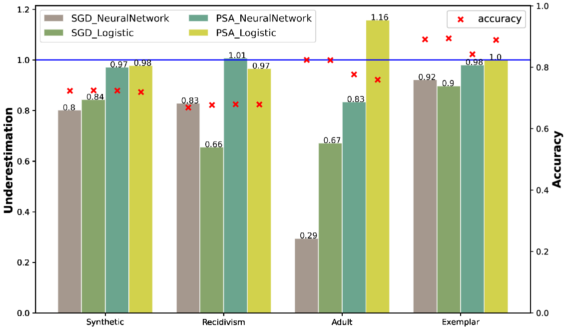
Figure 5.
 $US_{S=0}$
and accuracy scores for the four models on the test data.
$US_{S=0}$
and accuracy scores for the four models on the test data.
A UEI score of zero indicates that the model is predicting distributions that match those in the test data across all feature/class combinations. Figure 4 shows excellent results in these terms for the Synthetic, Recidivism and Exemplar datasets. The results for Adult are not perfect but are a significant improvement over the SGD models.
The
 $\mathrm{US}_{S=0}$
results are presented in Figure 5 to see how PSA is doing for the desirable outcome for the protected group, the thing we really care about. Bias against the protected group is effectively eliminated for all but the Adult dataset. Curiously, for this dataset,
$\mathrm{US}_{S=0}$
results are presented in Figure 5 to see how PSA is doing for the desirable outcome for the protected group, the thing we really care about. Bias against the protected group is effectively eliminated for all but the Adult dataset. Curiously, for this dataset,
 $\mathrm{PSA}_{Logistic}$
overshoots the mark while
$\mathrm{PSA}_{Logistic}$
overshoots the mark while
 $\mathrm{PSA}_{NeuralNetwork}$
falls significantly short.
$\mathrm{PSA}_{NeuralNetwork}$
falls significantly short.
Finally, it is interesting to note that these good underestimation results on the training data are achieved with very little loss in accuracy. The 1% to 2% impact on accuracy we see on the training data does not show up on the test data, perhaps because there is less overfitting.
6 Conclusion and future work
In this paper we present a multi-objective optimization strategy using Pareto Simulated Annealing that optimizes for both accuracy and underestimation. We demonstrate that our framework can achieve near-perfect underestimation as measured by UEI and
 $\mathrm{US}_{S=0}$
while maintaining adequate accuracy on three of the four datasets. On the fourth dataset (Adult) underestimation is improved a the cost of a small drop in accuracy.
$\mathrm{US}_{S=0}$
while maintaining adequate accuracy on three of the four datasets. On the fourth dataset (Adult) underestimation is improved a the cost of a small drop in accuracy.
For our future work we propose to extend this research in a number of areas:
-
Apply PSA to other learning models, for example naive Bayes and decision trees. Our formulation for applying PSA to logistic regression and neural networks is relatively straight forward. A similar strategy should also work for naive Bayes. However, developing a strategy for perturbing candidate solutions for decision trees (step 7 in Algorithm 1) will require some experimentation.
-
Evaluate other meta-heuristic strategies such as Particle Swarm Optimization (PSO). Would other methods be more effective for exploring very large parameter spaces?
-
Find other synthetic and real datasets to evaluate these methods.
Competing interests declaration
The authors declare none
Acknowledgements
This work was funded by Science Foundation Ireland through the SFI Centre for Research Training in Machine Learning (Grant No.18/CRT/6183) with support from Microsoft Ireland.


 Open access