


1 Introduction
Del Pezzo surfaces over $\mathbb {Q}$
often contain infinitely many rational points. Over the past 20 years, Manin’s conjecture [Reference Franke, Manin and Tschinkel16, Reference Peyre22] for the asymptotic behavior of the number of rational points of bounded anticanonical height has been confirmed for some smooth and many singular del Pezzo surfaces (see [Reference de la Bretèche4, Reference de la Bretèche, Browning and Derenthal5, Reference de la Bretèche, Browning and Peyre6] for some milestones and [Reference Arzhantsev, Derenthal, Hausen and Laface1, § 6.4.1] for many further references), in most cases using universal torsors, often combined with advanced analytic techniques.
$\mathbb {Q}$
often contain infinitely many rational points. Over the past 20 years, Manin’s conjecture [Reference Franke, Manin and Tschinkel16, Reference Peyre22] for the asymptotic behavior of the number of rational points of bounded anticanonical height has been confirmed for some smooth and many singular del Pezzo surfaces (see [Reference de la Bretèche4, Reference de la Bretèche, Browning and Derenthal5, Reference de la Bretèche, Browning and Peyre6] for some milestones and [Reference Arzhantsev, Derenthal, Hausen and Laface1, § 6.4.1] for many further references), in most cases using universal torsors, often combined with advanced analytic techniques.
In recent years, a conjectural framework for the density of integral points has emerged in the work of Chambert-Loir and Tschinkel [Reference Chambert-Loir and Tschinkel7]. The purpose of this paper is to initiate a systematic investigation of integral points of bounded height on del Pezzo surfaces. Only a few of them are covered by general results for equivariant compactifications of vector groups [Reference Chambert-Loir and Tschinkel8] or the incomplete work on toric varieties [Reference Chambert-Loir and Tschinkel9] (see also [Reference Wilsch25]); most del Pezzo surfaces are out of reach of this harmonic analysis approach since they are not equivariant compactifications of algebraic groups [Reference Derenthal and Loughran13, Reference Derenthal and Loughran14]. Del Pezzo surfaces are inaccessible to the circle method, which gives asymptotic formulas for integral points only on high-dimensional complete intersections [Reference Birch3], [Reference Chambert-Loir and Tschinkel7, § 5.4]. Therefore, we adapt the universal torsor method to integral points in order to confirm new cases of an integral analogue of Manin’s conjecture. See also [Reference Wilsch24] for a three-dimensional example.
As rational and integral points coincide on a projective variety X, the study of the latter becomes interesting on its own on an integral model of the complement $X\setminus Z$
of an appropriate boundary Z. Our first result (Theorem 10 in Section 2) is a general treatment of possible boundaries on singular del Pezzo surfaces of low degree. For singular cubic surfaces, Z must be an
$X\setminus Z$
of an appropriate boundary Z. Our first result (Theorem 10 in Section 2) is a general treatment of possible boundaries on singular del Pezzo surfaces of low degree. For singular cubic surfaces, Z must be an $\mathbf {A}$
-singularity; for singular quartic del Pezzo surfaces, Z must be an
$\mathbf {A}$
-singularity; for singular quartic del Pezzo surfaces, Z must be an $\mathbf {A}$
-singularity or a line passing only through
$\mathbf {A}$
-singularity or a line passing only through $\mathbf {A}$
-singularities. Furthermore,
$\mathbf {A}$
-singularities. Furthermore, $\mathbf {A}_1$
-singularities behave differently than other
$\mathbf {A}_1$
-singularities behave differently than other $\mathbf {A}$
-singularities.
$\mathbf {A}$
-singularities.
Therefore, a good starting point seems to be a quartic del Pezzo surface that contains an $\mathbf {A}_1$
- and an
$\mathbf {A}_1$
- and an $\mathbf {A}_3$
-singularity and three lines, which is neither toric [Reference Derenthal12, Remark 6] nor a compactification of
$\mathbf {A}_3$
-singularity and three lines, which is neither toric [Reference Derenthal12, Remark 6] nor a compactification of $\mathbb {G}_{\mathrm {a}}^2$
[Reference Derenthal and Loughran13]. For each boundary Z admissible in the sense of Theorem 10, we get an associated counting problem and prove an asymptotic formula of the shape
$\mathbb {G}_{\mathrm {a}}^2$
[Reference Derenthal and Loughran13]. For each boundary Z admissible in the sense of Theorem 10, we get an associated counting problem and prove an asymptotic formula of the shape
 $$\begin{align*}c B (\log B)^{b-1} \end{align*}$$
(Theorem 1), encountering a range of different phenomena when dealing with the different types of boundary. These asymptotic formulas admit a geometric interpretation (Theorem 2). In particular, the leading constant c consists of Tamagawa numbers as defined in [Reference Chambert-Loir and Tschinkel7] and combinatorial constants (analogous to the constant $\alpha $
defined by Peyre for rational points) as defined in [Reference Chambert-Loir and Tschinkel9] for toric varieties and studied in greater generality in [Reference Wilsch25]; this is the first result applying this combinatorial construction in a nontoric setting.
$\alpha $
defined by Peyre for rational points) as defined in [Reference Chambert-Loir and Tschinkel9] for toric varieties and studied in greater generality in [Reference Wilsch25]; this is the first result applying this combinatorial construction in a nontoric setting.
1.1 The counting problem
Let $S \subset \mathbb {P}^4_{\mathbb {Q}}$
be the quartic del Pezzo surface defined by
$S \subset \mathbb {P}^4_{\mathbb {Q}}$
be the quartic del Pezzo surface defined by
 $$ \begin{align} x_0^2+x_0x_3+x_2x_4=x_1x_3-x_2^2=0 \end{align} $$
over $\mathbb {Q}$
, with an
$\mathbb {Q}$
, with an $\mathbf {A}_1$
-singularity
$\mathbf {A}_1$
-singularity $Q_1=(0:1:0:0:0)$
and an
$Q_1=(0:1:0:0:0)$
and an $\mathbf {A}_3$
-singularity
$\mathbf {A}_3$
-singularity $Q_2=(0:0:0:0:1)$
. Let
$Q_2=(0:0:0:0:1)$
. Let $\mathcal {S} \subset \mathbb {P}^4_{\mathbb {Z}}$
be its integral model defined by the same equations over
$\mathcal {S} \subset \mathbb {P}^4_{\mathbb {Z}}$
be its integral model defined by the same equations over $\mathbb {Z}$
.
$\mathbb {Z}$
.
The closure of every rational point $P \in S(\mathbb {Q})$
is an integral point
$P \in S(\mathbb {Q})$
is an integral point $\overline {P} \in \mathcal {S}(\mathbb {Z})$
; both are represented (uniquely up to sign) by coprime
$\overline {P} \in \mathcal {S}(\mathbb {Z})$
; both are represented (uniquely up to sign) by coprime $(x_0,\dots ,x_4) \in \mathbb {Z}^5 \setminus \{0\}$
satisfying the defining equations (1). Recall that studying integral points becomes interesting only when we choose a boundary
$(x_0,\dots ,x_4) \in \mathbb {Z}^5 \setminus \{0\}$
satisfying the defining equations (1). Recall that studying integral points becomes interesting only when we choose a boundary $\mathcal {Z}$
to consider integral points on
$\mathcal {Z}$
to consider integral points on $\mathcal {S} \setminus \mathcal {Z}$
, and that the types of boundaries in Theorem 10 for our case are the singularities and the lines; we start with the former. To do so, let
$\mathcal {S} \setminus \mathcal {Z}$
, and that the types of boundaries in Theorem 10 for our case are the singularities and the lines; we start with the former. To do so, let $Z_1=Q_1$
,
$Z_1=Q_1$
, $Z_2=Q_2$
; in addition to these, we study the boundary
$Z_2=Q_2$
; in addition to these, we study the boundary $Z_3=Q_1\cup Q_2$
, which goes beyond the setting of weak del Pezzo pairs described in the beginning of the following section. Let
$Z_3=Q_1\cup Q_2$
, which goes beyond the setting of weak del Pezzo pairs described in the beginning of the following section. Let $\mathcal {Z}_i=\overline {Z_i}$
and
$\mathcal {Z}_i=\overline {Z_i}$
and $\mathcal {U}_i = \mathcal {S} \setminus \mathcal {Z}_i$
. Hence,
$\mathcal {U}_i = \mathcal {S} \setminus \mathcal {Z}_i$
. Hence, $\overline {P}$
lies in
$\overline {P}$
lies in $\mathcal {U}_3(\mathbb {Z})$
, say, if and only if it is does not reduce to one of the singularities modulo any prime p. In other words, a representative
$\mathcal {U}_3(\mathbb {Z})$
, say, if and only if it is does not reduce to one of the singularities modulo any prime p. In other words, a representative $(x_0,\dots ,x_4)$
of a point in
$(x_0,\dots ,x_4)$
of a point in $\mathcal {U}_i(\mathbb {Z})$
satisfies the integrality condition
$\mathcal {U}_i(\mathbb {Z})$
satisfies the integrality condition
 $$ \begin{align} \begin{aligned} \gcd(x_0,x_2,x_3,x_4)=1,\qquad &\text{if }i=1,\\ \gcd(x_0,x_1,x_2,x_3)=1,\qquad &\text{if }i=2, \text{ or}\\ \gcd(x_0,x_2,x_3,x_4)=1\quad\text{and}\quad \gcd(x_0,x_1,x_2,x_3)=1,\qquad &\text{if }i=3. \end{aligned} \end{align} $$
Since the sets $\mathcal {U}_i(\mathbb {Z})$
of integral points are clearly infinite, we consider integral points of bounded height. We work with the height functions
$\mathcal {U}_i(\mathbb {Z})$
of integral points are clearly infinite, we consider integral points of bounded height. We work with the height functions
 $$ \begin{align} \begin{aligned} H_1(\overline{P}) &=\max\{\left\lvert x_0\right\rvert,\left\lvert x_2\right\rvert,\left\lvert x_3\right\rvert,\left\lvert x_4\right\rvert\},\\ H_2(\overline{P}) &=\max\{\left\lvert x_0\right\rvert,\left\lvert x_1\right\rvert,\left\lvert x_2\right\rvert,\left\lvert x_3\right\rvert\},\qquad \text{and}\\ H_3(\overline{P}) &=\max\{\left\lvert x_0\right\rvert,\left\lvert x_2\right\rvert,\left\lvert x_3\right\rvert, \min\{\left\lvert x_1\right\rvert,\left\lvert x_4\right\rvert\}\} \end{aligned} \end{align} $$
because they can be interpreted as log-anticanonical heights on a minimal desingularization, as we shall see below (Lemma 14).
It turns out that the number of integral points of bounded height is dominated by the integral points on the three lines
 $$ \begin{align} L_1=\{x_0=x_2=x_3=0\},\ L_2=\{x_0=x_1=x_2=0\},\ L_3=\{x_0+x_3=x_1=x_2=0\}; \end{align} $$
in fact, there are infinitely many integral points of height $1$
on some of them. Therefore, we count integral points only in their complement
$1$
on some of them. Therefore, we count integral points only in their complement $V = S \setminus \{x_2=0\}$
. Hence, we are interested in the asymptotic behavior of
$V = S \setminus \{x_2=0\}$
. Hence, we are interested in the asymptotic behavior of
 $$ \begin{align} N_i(B) = \# \{\overline{P} \in \mathcal{U}_i(\mathbb{Z}) \cap V(\mathbb{Q}) \mid H_i(\overline{P}) \le B\}, \end{align} $$
the number of integral points of bounded log-anticanonical height that are not contained in the lines. Explicitly, this is
 $$ \begin{align} N_i(B) = \# \{(x_0,\dots,x_4) \in \mathbb{Z}^5 \setminus \{0\} \mid (1),\ (2),\ x_2> 0,\ H_i(x_0:\dots:x_4) \le B\}. \end{align} $$
Recall that the second type of boundary is a line, resulting in $Z_4=L_1,Z_5 = L_2, Z_6 \,{=}\, L_3$
with the notation in equation (4). Let
$Z_4=L_1,Z_5 = L_2, Z_6 \,{=}\, L_3$
with the notation in equation (4). Let $\mathcal {Z}_i=\overline {Z_i}$
in
$\mathcal {Z}_i=\overline {Z_i}$
in $\mathcal {S}$
and
$\mathcal {S}$
and $\mathcal {U}_i=\mathcal {S} \setminus \mathcal {Z}_i$
for
$\mathcal {U}_i=\mathcal {S} \setminus \mathcal {Z}_i$
for $i=4,5,6$
. Analogously to the first three cases, a point
$i=4,5,6$
. Analogously to the first three cases, a point $(x_0:\dots :x_4)\in S$
with coprime
$(x_0:\dots :x_4)\in S$
with coprime $x_0,\dots ,x_4 \in \mathbb {Z}$
lies in
$x_0,\dots ,x_4 \in \mathbb {Z}$
lies in $\mathcal {U}_i(\mathbb {Z})$
if and only if
$\mathcal {U}_i(\mathbb {Z})$
if and only if
 $$ \begin{align} \begin{aligned} \gcd(x_0,x_2,x_3)=1, \qquad &\text{if }i=4,\\ \gcd(x_0,x_1,x_2)=1, \qquad &\text{if }i=5, \text{ or}\\ \gcd(x_0+x_3,x_1,x_2)=1, \qquad &\text{if }i=6. \end{aligned} \end{align} $$
We work with the heights
 $$ \begin{align*} H_4(\overline{P}) &= \max\{|x_0|,|x_2|,|x_3|\},\\ H_5(\overline{P}) &= \max\{|x_0|,|x_1|,|x_2|\},\qquad \text{and}\\ H_6(\overline{P}) &= \max\{|x_0+x_3|,|x_1|,|x_2|\}, \end{align*} $$
which will again turn out to be log-anticanonical on a minimal desingularization. Let $N_i(B)$
for
$N_i(B)$
for $i=4,5,6$
be defined as in equation (5). They satisfy descriptions as in equation (6), with the integrality condition (2) replaced by condition (7).
$i=4,5,6$
be defined as in equation (5). They satisfy descriptions as in equation (6), with the integrality condition (2) replaced by condition (7).
Our second result consists of asymptotic formulas for these counting problems.
Theorem 1. As $B \to \infty $
, we have
$B \to \infty $
, we have
 $$ \begin{align*} N_1(B) &= \frac{13}{4320} \left(\prod_p \left(1-\frac 1 p\right)^5\left(1+\frac 5 p\right)\right) B (\log B)^5 + O(B (\log B)^4 \log\log B), \\ N_2(B) & = \frac{1}{32} \left(\prod_p \left(1-\frac 1 p\right)^3\left(1+\frac 3 p\right)\right) B (\log B)^4 + O(B(\log B)^3 \log\log B),\\ N_3(B) & = \frac 1 8 \left(\prod_p \left(1-\frac 1 p\right)^2\left(1+\frac 2 p-\frac 1 {p^2}\right)\right) B (\log B)^3 + O(B(\log B)^2 \log\log B), \\ N_4(B) &= 2 \left(\prod_p \left(1-\frac 1 p\right)\left(1+\frac 1 p\right)\right) B (\log B)^2 + O(B \log B \log\log B), \quad \text{and}\\ N_5(B) = N_6(B) &= \frac{7}{24} \left(\prod_p \left(1-\frac 1 p\right)^2\left(1+\frac 2 p\right)\right) B (\log B)^3 + O(B(\log B)^2 \log\log B). \end{align*} $$
Cases 5 and 6 are symmetric: the involutive automorphism
 $$ \begin{align} (x_0,x_1,x_2,x_3,x_4)\mapsto (x_0+x_3,-x_1,x_2,-x_3,x_4) \end{align} $$
of S exchanges the lines $L_2$
and
$L_2$
and $L_3$
and the height functions
$L_3$
and the height functions $H_5$
and
$H_5$
and $H_6$
, while leaving
$H_6$
, while leaving $V=S\setminus \{x_2=0\}$
invariant, whence
$V=S\setminus \{x_2=0\}$
invariant, whence $N_5(B)=N_6(B)$
.
$N_5(B)=N_6(B)$
.
1.2 The expected asymptotic formula
Similarly to the case of rational points [Reference Batyrev and Tschinkel2, Reference Peyre22], our asymptotic formulas for the number of integral points of bounded height should be interpreted on a desingularization $\rho \colon \widetilde {S} \to S$
. Here,
$\rho \colon \widetilde {S} \to S$
. Here, $\widetilde {S}$
is a weak del Pezzo surface, that is, a smooth projective surface whose anticanonical bundle
$\widetilde {S}$
is a weak del Pezzo surface, that is, a smooth projective surface whose anticanonical bundle $\omega _{\widetilde {S}}^\vee $
is big and nef (but not ample in our case).
$\omega _{\widetilde {S}}^\vee $
is big and nef (but not ample in our case).
To interpret the number of points on $\mathcal {U}_i = \mathcal {S} \setminus \mathcal {Z}_i$
, we study a desingularization
$\mathcal {U}_i = \mathcal {S} \setminus \mathcal {Z}_i$
, we study a desingularization $\widetilde {U}_i = \widetilde {S} \setminus D_i$
of
$\widetilde {U}_i = \widetilde {S} \setminus D_i$
of $U_i$
, where
$U_i$
, where $D_i=\rho ^{-1}(Z_i)$
is a reduced effective divisor with strict normal crossings. In the context of integral points, the log-anticanonical bundle
$D_i=\rho ^{-1}(Z_i)$
is a reduced effective divisor with strict normal crossings. In the context of integral points, the log-anticanonical bundle $\omega _{\widetilde {S}}(D_i)^\vee $
assumes the role of the anticanonical bundle. From this point of view, Theorem 1 can be interpreted in the framework described in [Reference Chambert-Loir and Tschinkel7].
$\omega _{\widetilde {S}}(D_i)^\vee $
assumes the role of the anticanonical bundle. From this point of view, Theorem 1 can be interpreted in the framework described in [Reference Chambert-Loir and Tschinkel7].
The minimal desingularization $\rho : \widetilde {S} \to S$
is an iterated blowup of
$\rho : \widetilde {S} \to S$
is an iterated blowup of $\mathbb {P}^2_{\mathbb {Q}}$
in five points. The analogous blowup of
$\mathbb {P}^2_{\mathbb {Q}}$
in five points. The analogous blowup of $\mathbb {P}^2_{\mathbb {Z}}$
results in an integral model
$\mathbb {P}^2_{\mathbb {Z}}$
results in an integral model $\rho \colon \widetilde {\mathcal {S}} \to \mathcal {S}$
(see section Section 3 for more details). Then
$\rho \colon \widetilde {\mathcal {S}} \to \mathcal {S}$
(see section Section 3 for more details). Then $D_1$
,
$D_1$
, $D_2$
are the divisors above
$D_2$
are the divisors above $Q_1,Q_2$
, respectively, and
$Q_1,Q_2$
, respectively, and $D_3=D_1+D_2$
is the one over both; see Figure 1 for their dual graph (Dynkin diagram). Our discussion is simplified by the fact that the pairs
$D_3=D_1+D_2$
is the one over both; see Figure 1 for their dual graph (Dynkin diagram). Our discussion is simplified by the fact that the pairs $(\widetilde {S},D_i)$
are split, in the sense that
$(\widetilde {S},D_i)$
are split, in the sense that $\operatorname {\mathrm {Pic}}\widetilde {S} \to \operatorname {\mathrm {Pic}}\widetilde {S}_{\overline {\mathbb {Q}}}$
is an isomorphism and [Reference Harpaz18, Definition 1.6] holds, and by the fact that we are working over
$\operatorname {\mathrm {Pic}}\widetilde {S} \to \operatorname {\mathrm {Pic}}\widetilde {S}_{\overline {\mathbb {Q}}}$
is an isomorphism and [Reference Harpaz18, Definition 1.6] holds, and by the fact that we are working over $\mathbb {Q}$
. Let
$\mathbb {Q}$
. Let $\widetilde {U}_i,\widetilde {\mathcal {U}}_i$
be the complement of
$\widetilde {U}_i,\widetilde {\mathcal {U}}_i$
be the complement of $D_i,\overline {D_i}$
in
$D_i,\overline {D_i}$
in $\widetilde {S},\widetilde {\mathcal {S}}$
, respectively, where
$\widetilde {S},\widetilde {\mathcal {S}}$
, respectively, where $\overline {D_i}$
is the Zariski closure of
$\overline {D_i}$
is the Zariski closure of $D_i$
in
$D_i$
in $\widetilde {\mathcal {S}}$
. The preimage of the complement V of the lines on S is the complemenent
$\widetilde {\mathcal {S}}$
. The preimage of the complement V of the lines on S is the complemenent $\widetilde {V}$
of all negative curves on
$\widetilde {V}$
of all negative curves on $\widetilde {S}$
.
$\widetilde {S}$
.
This leads to the reinterpretation of our counting problem as
 $$ \begin{align*} N_i(B) = \#\{\overline{P} \in \widetilde{\mathcal{U}}_i(\mathbb{Z}) \cap \widetilde{V}(\mathbb{Q}) \mid H_i(\rho(\overline{P})) \le B\} \end{align*} $$
on the minimal desingularization, and we prove in Lemma 14 that $H_i \circ \rho $
is a log-anticanonical height function on
$H_i \circ \rho $
is a log-anticanonical height function on $\widetilde {\mathcal {U}}_i(\mathbb {Z}) \cap \widetilde {V}(\mathbb {Q})$
. Note that the log-anticanonical bundle
$\widetilde {\mathcal {U}}_i(\mathbb {Z}) \cap \widetilde {V}(\mathbb {Q})$
. Note that the log-anticanonical bundle $\omega _{\widetilde {S}}(D_i)^\vee $
is big and nef for
$\omega _{\widetilde {S}}(D_i)^\vee $
is big and nef for $i=1,2,4,5,6$
but big and not nef for
$i=1,2,4,5,6$
but big and not nef for $i=3$
(Lemma 12); the unusual shape of
$i=3$
(Lemma 12); the unusual shape of $H_3$
is clearly related to this.
$H_3$
is clearly related to this.
From the shape of asymptotic formulas in previous results [Reference Chambert-Loir and Tschinkel9, Reference Chambert-Loir and Tschinkel8, Reference Takloo-Bighash and Tschinkel23, Reference Wilsch24] and the study of volume asymptotics in [Reference Chambert-Loir and Tschinkel7], we expect that
 $$ \begin{align*} N_i(B) \sim c_{i,\mathrm{fin}}c_{i,\infty} B (\log B)^{b_i-1}, \end{align*} $$
where the leading constant can be decomposed into a finite part $c_{i,\mathrm {fin}}$
and an Archimedean part
$c_{i,\mathrm {fin}}$
and an Archimedean part $c_{i,\infty }$
that we shall describe and determine in Section 6 precisely.
$c_{i,\infty }$
that we shall describe and determine in Section 6 precisely.
The finite part
 $$ \begin{align} c_{i,\mathrm{fin}} = \prod_p \left(1-\frac 1 p \right)^{\operatorname{\mathrm{rk}}\operatorname{\mathrm{Pic}}\widetilde{U}_i} \tau_{(\widetilde{S},D_i), p}(\widetilde{\mathcal{U}}_i(\mathbb{Z}_p)), \end{align} $$
which behaves similarly as in the case of rational points, is defined as an Euler product of convergence factors and p-adic Tamagawa numbers. We compute the latter as p-adic integrals over $\widetilde {\mathcal {U}}_i(\mathbb {Z}_p)$
(Lemma 24); they turn out to be simply
$\widetilde {\mathcal {U}}_i(\mathbb {Z}_p)$
(Lemma 24); they turn out to be simply $\#\widetilde {\mathcal {U}}_i(\mathbb {F}_p)/p^{\dim S}$
. This reflects the fact that integral points should be distributed evenly in the set
$\#\widetilde {\mathcal {U}}_i(\mathbb {F}_p)/p^{\dim S}$
. This reflects the fact that integral points should be distributed evenly in the set $\widetilde {\mathcal {U}}_i(\mathbb {Z}_p)$
, which has positive and finite volume with respect to the modified Tamagawa measure
$\widetilde {\mathcal {U}}_i(\mathbb {Z}_p)$
, which has positive and finite volume with respect to the modified Tamagawa measure $\tau _{(\widetilde {S},D_i),p}$
defined in [Reference Chambert-Loir and Tschinkel7]. (However, we do not prove such an equidistribution result here.)
$\tau _{(\widetilde {S},D_i),p}$
defined in [Reference Chambert-Loir and Tschinkel7]. (However, we do not prove such an equidistribution result here.)
On the other hand, 100% of the integral points are arbitrarily close to the boundary with respect to the real-analytic topology, ordered by height. This makes the analysis of $c_{i,\infty }$
much more delicate than for rational points. More precisely, the points close to the minimal strata of the boundary—that is, the intersection of a maximal set of intersecting components of
$c_{i,\infty }$
much more delicate than for rational points. More precisely, the points close to the minimal strata of the boundary—that is, the intersection of a maximal set of intersecting components of $D_i$
—should dominate the counting function. These strata are encoded in the (analytic) Clemens complex
$D_i$
—should dominate the counting function. These strata are encoded in the (analytic) Clemens complex $\mathcal {C}^{\mathrm {an}}_{\mathbb {R}}(D_i)$
. For a split surface, the vertices of this Clemens complex correspond to the irreducible components of the boundary divisor
$\mathcal {C}^{\mathrm {an}}_{\mathbb {R}}(D_i)$
. For a split surface, the vertices of this Clemens complex correspond to the irreducible components of the boundary divisor $D_i$
, and there is an edge for each intersection point of two divisors. The Archimedean constant
$D_i$
, and there is an edge for each intersection point of two divisors. The Archimedean constant
 $$ \begin{align} c_{i,\infty} = \sum_A \alpha_{i,A} \tau_{i,D_A,\infty}(D_A(\mathbb{R})) \end{align} $$
is a sum over the faces A of maximal dimension of the Clemens complex, which correspond to the minimal strata $D_A$
of
$D_A$
of $D_i$
. For each maximal-dimensional face A, we have a product of a rational factor
$D_i$
. For each maximal-dimensional face A, we have a product of a rational factor $\alpha _{i,A}$
and an Archimedean Tamagawa number
$\alpha _{i,A}$
and an Archimedean Tamagawa number $\tau _{i,D_A,\infty }(D_A(\mathbb {R}))$
coming from a residue measure as defined in [Reference Chambert-Loir and Tschinkel7]. This measure can be interpreted as a real density, which is supported on
$\tau _{i,D_A,\infty }(D_A(\mathbb {R}))$
coming from a residue measure as defined in [Reference Chambert-Loir and Tschinkel7]. This measure can be interpreted as a real density, which is supported on $D_A(\mathbb {R})$
and should measure the distribution of points in neighborhoods of open subsets of
$D_A(\mathbb {R})$
and should measure the distribution of points in neighborhoods of open subsets of $D_A(\mathbb {R})$
. From another point of view, the set
$D_A(\mathbb {R})$
. From another point of view, the set $\widetilde {S}(\mathbb {R})$
has infinite volume with respect to a modified measure
$\widetilde {S}(\mathbb {R})$
has infinite volume with respect to a modified measure $\tau _{(\widetilde {S},D_i),\infty }$
as above, and
$\tau _{(\widetilde {S},D_i),\infty }$
as above, and $\tau _{i,D_A,\infty }(D_A(\mathbb {R}))$
appears in the leading constant of the asymptotic volume of height balls with respect to said measure (cf. [Reference Chambert-Loir and Tschinkel7, Propositions 2.5.1, 4.2.4]).
$\tau _{i,D_A,\infty }(D_A(\mathbb {R}))$
appears in the leading constant of the asymptotic volume of height balls with respect to said measure (cf. [Reference Chambert-Loir and Tschinkel7, Propositions 2.5.1, 4.2.4]).
In the first case, the Clemens complex consists of only one vertex corresponding to the boundary divisor above the $\mathbf {A}_1$
-singularity
$\mathbf {A}_1$
-singularity $Q_1$
, and integral points accumulate near it (Figure 2). In the second and third case, the maximal-dimensional faces
$Q_1$
, and integral points accumulate near it (Figure 2). In the second and third case, the maximal-dimensional faces $A_1,A_2$
of the Clemens complex correspond to the two intersection points
$A_1,A_2$
of the Clemens complex correspond to the two intersection points $D_{A_1},D_{A_2}$
of the divisors above the
$D_{A_1},D_{A_2}$
of the divisors above the $\mathbf {A}_3$
-singularity, and ‘most’ integral points are very close to these two intersection points (Figure 3). Correspondingly, the Archimedean Tamagawa number is the volume of the boundary divisor in the first case, and it is the volume of the two intersection points in the second and third cases. In the remaining cases, it similarly is a volume of intersection points (Lemma 25).
$\mathbf {A}_3$
-singularity, and ‘most’ integral points are very close to these two intersection points (Figure 3). Correspondingly, the Archimedean Tamagawa number is the volume of the boundary divisor in the first case, and it is the volume of the two intersection points in the second and third cases. In the remaining cases, it similarly is a volume of intersection points (Lemma 25).
Figure 1 The Clemens complex of $D_3$
is the disjoint union of those of
$D_3$
is the disjoint union of those of $D_1$
(left) and
$D_1$
(left) and $D_2$
(right). It is the Dynkin diagram of the
$D_2$
(right). It is the Dynkin diagram of the $\mathbf {A}_1$
- and
$\mathbf {A}_1$
- and $\mathbf {A}_3$
-singularities
$\mathbf {A}_3$
-singularities $Q_1,Q_2$
.
$Q_1,Q_2$
.
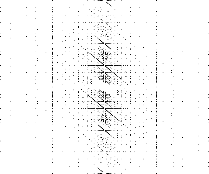
Figure 2 Integral points on $\widetilde {\mathcal {U}}_1$
of height
$\widetilde {\mathcal {U}}_1$
of height $\le 90$
. The boundary divisor is the central vertical line. Some horizontal and diagonal lines look accumulating, but in fact are not: They contain
$\le 90$
. The boundary divisor is the central vertical line. Some horizontal and diagonal lines look accumulating, but in fact are not: They contain $\sim c^\prime B$
points, which is less than the
$\sim c^\prime B$
points, which is less than the $c B(\log B)^5$
points on U; the constants
$c B(\log B)^5$
points on U; the constants $c^\prime $
can however be up to
$c^\prime $
can however be up to $2$
, while the constant c in our main theorem is numerically
$2$
, while the constant c in our main theorem is numerically $\approx 0.0003$
.
$\approx 0.0003$
.

Figure 3 Integral points on $\widetilde {\mathcal {U}}_2$
of height
$\widetilde {\mathcal {U}}_2$
of height $\le 60$
in neighborhoods of
$\le 60$
in neighborhoods of $D_{A_1}$
(left) and
$D_{A_1}$
(left) and $D_{A_2}$
(right). Most points are close to the three boundary divisors, which are the central horizontal line and two vertical lines here.
$D_{A_2}$
(right). Most points are close to the three boundary divisors, which are the central horizontal line and two vertical lines here.
The rational factor $\alpha _{i,A}$
is particularly interesting in our examples. It is introduced in [Reference Chambert-Loir and Tschinkel9] for toric varieties and generalized in [Reference Wilsch25] to be
$\alpha _{i,A}$
is particularly interesting in our examples. It is introduced in [Reference Chambert-Loir and Tschinkel9] for toric varieties and generalized in [Reference Wilsch25] to be
 $$ \begin{align} \alpha_{i,A} = \operatorname{\mathrm{vol}}\{x \in (\operatorname{\mathrm{Eff}}\widetilde{U}_{i,A})^\vee \mid \langle x, \omega_{\widetilde{S}}(D_i)^\vee|_{\widetilde{U}_{i,A}}\rangle = 1\}, \end{align} $$
where $\widetilde {U}_{i,A}$
is the subvariety consisting of
$\widetilde {U}_{i,A}$
is the subvariety consisting of $\widetilde {U}_i$
and the divisors corresponding to A. For vector groups [Reference Chambert-Loir and Tschinkel8] and wonderful compactifications [Reference Takloo-Bighash and Tschinkel23], the effective cone is generated by the boundary divisors and simplicial, which makes the treatment of this factor easy. In [Reference Wilsch24], it behaves similarly as Peyre’s
$\widetilde {U}_i$
and the divisors corresponding to A. For vector groups [Reference Chambert-Loir and Tschinkel8] and wonderful compactifications [Reference Takloo-Bighash and Tschinkel23], the effective cone is generated by the boundary divisors and simplicial, which makes the treatment of this factor easy. In [Reference Wilsch24], it behaves similarly as Peyre’s $\alpha $
for projective varieties since the boundary has just one component; it is also much simpler since the Picard number is
$\alpha $
for projective varieties since the boundary has just one component; it is also much simpler since the Picard number is $2$
. Our second and following cases behave in a different way since the Clemens complex is not a simplex, providing the first nontrivial treatment of this factor for a nontoric variety. Here, it turns out that the resulting polytopes for the different maximal faces fit together to one polytope whose volume appears in the leading constant of the counting problem (Lemma 28). In case
$2$
. Our second and following cases behave in a different way since the Clemens complex is not a simplex, providing the first nontrivial treatment of this factor for a nontoric variety. Here, it turns out that the resulting polytopes for the different maximal faces fit together to one polytope whose volume appears in the leading constant of the counting problem (Lemma 28). In case $4$
, one of the polytopes has volume
$4$
, one of the polytopes has volume $0$
, making this an example for the obstruction [Reference Wilsch25, Theorem 2.4.1 (i)] to the existence of integral points near the corresponding minimal stratum of the boundary (Remark 27).
$0$
, making this an example for the obstruction [Reference Wilsch25, Theorem 2.4.1 (i)] to the existence of integral points near the corresponding minimal stratum of the boundary (Remark 27).
The exponent of $\log B$
is expected to be
$\log B$
is expected to be $b_i-1$
, where
$b_i-1$
, where
 $$ \begin{align} b_i = \operatorname{\mathrm{rk}}\operatorname{\mathrm{Pic}}\widetilde{U}_i - \operatorname{\mathrm{rk}} \mathbb{Q}[U_i]/\mathbb{Q}^\times + \dim \mathcal{C}^{\mathrm{an}}_{\mathbb{R}}(D_i) + 1. \end{align} $$
Here, $\dim \mathcal {C}^{\mathrm {an}}_{\mathbb {R}}(D_i) + 1$
is the maximal number of components of the boundary divisor
$\dim \mathcal {C}^{\mathrm {an}}_{\mathbb {R}}(D_i) + 1$
is the maximal number of components of the boundary divisor $D_i$
that meet in the same point, and
$D_i$
that meet in the same point, and $\mathbb {Q}[U_i]^\times = \mathbb {Q}^\times $
in each case. While the obstruction described in [Reference Wilsch25] can lead to this number being smaller than expected if it affects all maximal-dimensional faces of the Clemens complex, this does not happen in our fourth case as there are three unobstructed faces remaining.
$\mathbb {Q}[U_i]^\times = \mathbb {Q}^\times $
in each case. While the obstruction described in [Reference Wilsch25] can lead to this number being smaller than expected if it affects all maximal-dimensional faces of the Clemens complex, this does not happen in our fourth case as there are three unobstructed faces remaining.
We can reformulate Theorem 1 as follows.
Theorem 2. For $i \in \{1,\dots ,6\}$
, we have
$i \in \{1,\dots ,6\}$
, we have
 $$ \begin{align} N_i(B) = c_{i,\infty} c_{i,\mathrm{fin}} B(\log B)^{b_i-1}(1+o(1)) \end{align} $$
as $B \to \infty $
, where the constants
$B \to \infty $
, where the constants $c_{i,\infty }$
,
$c_{i,\infty }$
, $c_{i,\mathrm {fin}}$
and
$c_{i,\mathrm {fin}}$
and $b_i$
are as in equations (9), (10) and (12), respectively.
$b_i$
are as in equations (9), (10) and (12), respectively.
This confirms the expectations extracted from [Reference Chambert-Loir and Tschinkel7, Reference Chambert-Loir and Tschinkel9, Reference Wilsch25].
1.3 Strategy of the proof
In Section 2, we define and classify weak del Pezzo pairs $(\widetilde {S},D)$
, which have big and nef log-anticanonical bundle
$(\widetilde {S},D)$
, which have big and nef log-anticanonical bundle $\omega _{\widetilde {S}}(D)^\vee $
(Theorem 10).
$\omega _{\widetilde {S}}(D)^\vee $
(Theorem 10).
In Section 3, we describe a universal torsor on the minimal desingularization of S, we show that our height functions are log-anticanonical, and we describe them in terms of Cox coordinates. This leads to a completely explicit counting problem on the universal torsor (Lemma 15), with a $(2^{\operatorname {\mathrm {rk}}\operatorname {\mathrm {Pic}}\widetilde {U}_i}:1)$
-map to our set of integral points of bounded height: roughly, the torsor variables corresponding to the boundary divisors must be
$(2^{\operatorname {\mathrm {rk}}\operatorname {\mathrm {Pic}}\widetilde {U}_i}:1)$
-map to our set of integral points of bounded height: roughly, the torsor variables corresponding to the boundary divisors must be $\pm 1$
, and in the case of a big and base point free (whence nef) log-anticanonical class, the height function
$\pm 1$
, and in the case of a big and base point free (whence nef) log-anticanonical class, the height function $H_i$
is given by monomials in the Cox ring of log-anticanonical degree. The third case seems to be one of the first examples of the universal torsor method with respect to a height for a divisor class that is big and not nef.
$H_i$
is given by monomials in the Cox ring of log-anticanonical degree. The third case seems to be one of the first examples of the universal torsor method with respect to a height for a divisor class that is big and not nef.
In Section 4, we estimate the number of points in our counting problem on the universal torsor using analytic techniques. Here, we approximate summations over the torsor variables by real integrals $V_{i,0}(B)$
; the coprimality conditions lead to an Euler product that agrees with
$V_{i,0}(B)$
; the coprimality conditions lead to an Euler product that agrees with $c_{i,\mathrm {fin}}$
(Lemmas 16 and 17). This step is similar to the case of rational points treated in [Reference Derenthal11]; hence, we shall be very brief.
$c_{i,\mathrm {fin}}$
(Lemmas 16 and 17). This step is similar to the case of rational points treated in [Reference Derenthal11]; hence, we shall be very brief.
In Section 5, to complete the proof of Theorem 1, our goal is to transform $V_{i,0}(B)$
into
$V_{i,0}(B)$
into $2^{\operatorname {\mathrm {rk}}\operatorname {\mathrm {Pic}}\widetilde {U}_i} C_i B(\log B)^{b_i-1}$
, where
$2^{\operatorname {\mathrm {rk}}\operatorname {\mathrm {Pic}}\widetilde {U}_i} C_i B(\log B)^{b_i-1}$
, where $C_i$
is the product of the volume of a polytope (which turns out to be
$C_i$
is the product of the volume of a polytope (which turns out to be $\sum \alpha _{i,A}$
) and a real density (which agrees with the Archimedean Tamagawa numbers
$\sum \alpha _{i,A}$
) and a real density (which agrees with the Archimedean Tamagawa numbers $\tau _{i,D_A,\infty }(D_A(\mathbb {R}))$
), up to a negligible error term. In the first case, there is a complication due to an inhomogeneous expression (with respect to the grading by the Picard group) in the domain of
$\tau _{i,D_A,\infty }(D_A(\mathbb {R}))$
), up to a negligible error term. In the first case, there is a complication due to an inhomogeneous expression (with respect to the grading by the Picard group) in the domain of $V_{1,0}$
(Lemma 18 and more importantly Lemma 19); here, a subtle estimation is necessary. In the third case, we modify the height function
$V_{1,0}$
(Lemma 18 and more importantly Lemma 19); here, a subtle estimation is necessary. In the third case, we modify the height function $H_3$
to
$H_3$
to $H_3'$
(which coincides essentially with
$H_3'$
(which coincides essentially with $H_2$
) as in Lemma 20. These extra complications have never appeared in the universal torsor method for rational points; we believe that they are typical for integral points and nonnef heights.
$H_2$
) as in Lemma 20. These extra complications have never appeared in the universal torsor method for rational points; we believe that they are typical for integral points and nonnef heights.
In Section 6, we prove Theorem 2 by explicitly computing the expected constants discussed in Section 1.2.
2 Classification of weak del Pezzo pairs
For us, a weak del Pezzo pair $(\widetilde {S},D)$
consists of a smooth projective surface
$(\widetilde {S},D)$
consists of a smooth projective surface $\widetilde {S}$
with a reduced effective divisor D with strict normal crossings such that the log-anticanonical bundle
$\widetilde {S}$
with a reduced effective divisor D with strict normal crossings such that the log-anticanonical bundle $\omega _{\widetilde {S}}(D)^\vee $
is big and nef. The aim of this section is to study the possible choices of divisors D on a weak del Pezzo surface
$\omega _{\widetilde {S}}(D)^\vee $
is big and nef. The aim of this section is to study the possible choices of divisors D on a weak del Pezzo surface $\widetilde {S}$
that render the pair
$\widetilde {S}$
that render the pair $(\widetilde {S},D)$
weak del Pezzo in this sense.
$(\widetilde {S},D)$
weak del Pezzo in this sense.
Remark 3. Considering pairs $(X,D)$
is standard when studying integral points: While rational and integral points coincide on complete varieties as a consequence of the valuative criterion for properness, the study of integral points becomes a distinct problem on an integral model
$(X,D)$
is standard when studying integral points: While rational and integral points coincide on complete varieties as a consequence of the valuative criterion for properness, the study of integral points becomes a distinct problem on an integral model $\mathcal {U}$
of a noncomplete variety U. Then one passes to a compactification, more precisely, a smooth projective variety X containing U such that the boundary
$\mathcal {U}$
of a noncomplete variety U. Then one passes to a compactification, more precisely, a smooth projective variety X containing U such that the boundary $D = X \setminus U$
is a reduced effective divisor with strict normal crossings. In particular, the pair
$D = X \setminus U$
is a reduced effective divisor with strict normal crossings. In particular, the pair $(X,D)$
is smooth and divisorially log terminal.
$(X,D)$
is smooth and divisorially log terminal.
The goal is then to count the number of points on $\mathcal {U}$
of bounded log-anticanonical height (that is, with respect to
$\mathcal {U}$
of bounded log-anticanonical height (that is, with respect to $\omega _X(D)^\vee $
), excluding any strict subvarieties (or, more generally, thin subsets) whose points would contribute to the main term. Setting
$\omega _X(D)^\vee $
), excluding any strict subvarieties (or, more generally, thin subsets) whose points would contribute to the main term. Setting $D=0$
then recovers the setting of Manin’s conjecture on rational points.
$D=0$
then recovers the setting of Manin’s conjecture on rational points.
Remark 4. In its original form [Reference Franke, Manin and Tschinkel16, Reference Peyre21], Manin’s conjecture makes a prediction about the number of rational points on smooth Fano varieties: smooth projective varieties whose anticanonical bundle is ample. These conditions can be relaxed—for example, only requiring that the anticanonical be big and nef, viz. to weak Fano varieties and the two-dimensional varieties thereof, weak del Pezzo surfaces. Weak del Pezzo surfaces $\widetilde {S}$
are precisely the smooth del Pezzo surfaces
$\widetilde {S}$
are precisely the smooth del Pezzo surfaces $\widetilde {S} = S$
and the minimal desingularizations
$\widetilde {S} = S$
and the minimal desingularizations $\rho \colon \widetilde {S}\to S$
of del Pezzo surfaces with only
$\rho \colon \widetilde {S}\to S$
of del Pezzo surfaces with only $\mathbf {ADE}$
-singularities [Reference Demazure10].
$\mathbf {ADE}$
-singularities [Reference Demazure10].
Since $\rho $
is a crepant resolution—that is,
$\rho $
is a crepant resolution—that is, $\omega _{\widetilde {S}} = \rho ^* \omega _S$
—counting points on S of bounded anticanonical height amounts to counting points on
$\omega _{\widetilde {S}} = \rho ^* \omega _S$
—counting points on S of bounded anticanonical height amounts to counting points on $\widetilde {S}$
of bounded anticanonical height after excluding points on the exceptional locus. By [Reference Batyrev and Tschinkel2, Reference Peyre22], an asymptotic formula for the number of rational points on S should be interpreted in terms of its minimal desingularization
$\widetilde {S}$
of bounded anticanonical height after excluding points on the exceptional locus. By [Reference Batyrev and Tschinkel2, Reference Peyre22], an asymptotic formula for the number of rational points on S should be interpreted in terms of its minimal desingularization $\widetilde {S}$
; for example, the Picard rank
$\widetilde {S}$
; for example, the Picard rank $\rho $
of
$\rho $
of $\widetilde {S}$
appears in the expected asymptotic formula. The number of rational points of bounded height has been shown to conform to the same prediction as in Manin’s conjecture for many weak del Pezzo surfaces (see the references in [Reference Arzhantsev, Derenthal, Hausen and Laface1, § 6.4.1]).
$\widetilde {S}$
appears in the expected asymptotic formula. The number of rational points of bounded height has been shown to conform to the same prediction as in Manin’s conjecture for many weak del Pezzo surfaces (see the references in [Reference Arzhantsev, Derenthal, Hausen and Laface1, § 6.4.1]).
Generalizing the question even further, it suffices to assume that the anticanonical bundle is big to guarantee that the number of rational points of bounded anticanonical height outside a suitable divisor is finite. Adding some conditions that make Peyre’s constant well-defined leads to the notion of an almost Fano variety [Reference Peyre22, Définition 3.1], for which it makes sense to ask whether Manin’s conjecture holds. While this is known to be the case for some of them, Lehmann, Sengupta, and Tanimoto showed that one cannot expect the conjecture to be true in general in this widest setting [Reference Lehmann, Sengupta and Tanimoto19, Remark 1.1, Example 5.17].
To simplify the exposition, let $\widetilde {S}$
be a weak del Pezzo surface whose degree d is at most
$\widetilde {S}$
be a weak del Pezzo surface whose degree d is at most $7$
. Let
$7$
. Let $D=\sum _{\alpha \in \mathcal {A}} D_\alpha \subset \widetilde {S}$
be a reduced and effective divisor with strict normal crossings and irreducible components
$D=\sum _{\alpha \in \mathcal {A}} D_\alpha \subset \widetilde {S}$
be a reduced and effective divisor with strict normal crossings and irreducible components $D_\alpha $
.
$D_\alpha $
.
Lemma 5. The log-anticanonical bundle $\omega _{\widetilde {S}}(D)^\vee $
is nef if and only if all of the following conditions hold:
$\omega _{\widetilde {S}}(D)^\vee $
is nef if and only if all of the following conditions hold:
-
(i) If E is a $(-2)$
-curve and
$D_\alpha .E>0$
for some
$\alpha \in \mathcal {A}$
, then
$E \subset D$
.
$(-2)$
-curve and
$D_\alpha .E>0$
for some
$\alpha \in \mathcal {A}$
, then
$E \subset D$
. -
(ii) If E is an arbitrary negative curve meeting two different
$D_\alpha ,D_\beta $
or one
$D_\gamma \subset D$
with multiplicity
$D_\gamma .E\ge 2$
(with
$\alpha ,\beta ,\gamma \in \mathcal {A}$
), then
$E \subset D$
. -
(iii) If E is a negative curve, then
$$\begin{align*}\sum_{\substack{\alpha \in \mathcal{A} \\ D_\alpha \ne E }} D_\alpha. E \le 2. \end{align*}$$


Proof. Recall that a divisor is nef if its intersection with all negative curves is nonnegative. If E is a $(-2)$
-curve, then
$(-2)$
-curve, then
 $$\begin{align*}(-K-D).E = -K.E-D.E = 0 + 2\delta_{E \subset D} - \sum_{\substack{\alpha \in \mathcal{A} \\ D_\alpha \ne E }}D_\alpha. E, \end{align*}$$
and this number is nonnegative if and only if (i) and (iii) hold for E. If E is a $(-1)$
-curve, then
$(-1)$
-curve, then
 $$\begin{align*}(-K-D).E = -K.E-D.E = 1 + \delta_{E \in D} - \sum_{\substack{\alpha \in \mathcal{A} \\ D_\alpha \ne E }}D_\alpha. E, \end{align*}$$
and this number is nonnegative if and only if (ii) and (iii) hold for E.
Remark 6. If $\rho \colon \widetilde {S}\to S$
is the minimal desingularization of a singular del Pezzo surface, then Lemma 5 shows: If one of the
$\rho \colon \widetilde {S}\to S$
is the minimal desingularization of a singular del Pezzo surface, then Lemma 5 shows: If one of the $(-2)$
-curves above a singularity
$(-2)$
-curves above a singularity $Q \in S$
is in D, then by Lemma 5 (i) all curves above this singularity must be in D. Similarly, if a
$Q \in S$
is in D, then by Lemma 5 (i) all curves above this singularity must be in D. Similarly, if a $(-1)$
-curve whose image in S contains a singularity Q is in D, then all
$(-1)$
-curve whose image in S contains a singularity Q is in D, then all $(-2)$
-curves above Q must be in D. By Lemma 5 (iii), Q must be an
$(-2)$
-curves above Q must be in D. By Lemma 5 (iii), Q must be an $\mathbf {A}$
-singularity in both cases.
$\mathbf {A}$
-singularity in both cases.
The surface $\widetilde {S}$
can be described by a sequence of
$\widetilde {S}$
can be described by a sequence of $r=9-\deg \widetilde {S}$
blowups
$r=9-\deg \widetilde {S}$
blowups
 $$ \begin{align*} \widetilde{S} = \widetilde{S}^{(r)} \xrightarrow{\pi_r} \widetilde{S}^{(r-1)}\to \dots \to \widetilde{S}^{(1)} \xrightarrow{\pi_1} \widetilde{S}^{(0)} = \mathbb{P}^2, \end{align*} $$
where $\pi _i$
is the blowup in a point
$\pi _i$
is the blowup in a point $p_i$
that does not lie on a
$p_i$
that does not lie on a $(-2)$
-curve on
$(-2)$
-curve on $\widetilde {S}^{(i-1)}$
. Let
$\widetilde {S}^{(i-1)}$
. Let $\pi \colon \widetilde {S} \to \mathbb {P}^2$
be their composition. Let
$\pi \colon \widetilde {S} \to \mathbb {P}^2$
be their composition. Let $\ell _0=\pi ^*\ell $
, where
$\ell _0=\pi ^*\ell $
, where $\ell $
is the class of a line on
$\ell $
is the class of a line on $\mathbb {P}^2$
, and for
$\mathbb {P}^2$
, and for $1\le i\le r$
, let
$1\le i\le r$
, let $\ell _i=(\pi _{i+1}\cdots \pi _{r})^{*}E^{(i)}$
, where
$\ell _i=(\pi _{i+1}\cdots \pi _{r})^{*}E^{(i)}$
, where $E^{(i)}$
is the exceptional divisor of the ith blowup
$E^{(i)}$
is the exceptional divisor of the ith blowup $\pi _i$
. Then the Picard group of
$\pi _i$
. Then the Picard group of $\widetilde {S}$
is freely generated by the classes
$\widetilde {S}$
is freely generated by the classes $\ell _0,\dots ,\ell _r$
. The intersection form is given by
$\ell _0,\dots ,\ell _r$
. The intersection form is given by $\ell _i.\ell _j=0$
for
$\ell _i.\ell _j=0$
for $i\ne j$
,
$i\ne j$
, $\ell _0^2=1$
, and
$\ell _0^2=1$
, and $\ell _i^2=-1$
for
$\ell _i^2=-1$
for $i\ge 1$
. Let P be the image of an exceptional divisor of one of the the blowups in
$i\ge 1$
. Let P be the image of an exceptional divisor of one of the the blowups in $\mathbb {P}^2$
and
$\mathbb {P}^2$
and $n_P$
be the number of exceptional curves mapped to P. Then these negative curves form a chain, the first
$n_P$
be the number of exceptional curves mapped to P. Then these negative curves form a chain, the first $n_P-1$
of which are
$n_P-1$
of which are $(-2)$
-curves whose classes have the form
$(-2)$
-curves whose classes have the form $\ell _{i_1} - \ell _{i_2}$
, …,
$\ell _{i_1} - \ell _{i_2}$
, …, $\ell _{i_{s-1}}-\ell _{i_s}$
followed by a
$\ell _{i_{s-1}}-\ell _{i_s}$
followed by a $(-1)$
-curve whose class has the form
$(-1)$
-curve whose class has the form $\ell _{i_s}$
. The anticanonical class is
$\ell _{i_s}$
. The anticanonical class is $3\ell _0 - \ell _1 - \cdots - \ell _r$
, and we fix an anticanonical divisor
$3\ell _0 - \ell _1 - \cdots - \ell _r$
, and we fix an anticanonical divisor $-K$
. Denote by
$-K$
. Denote by $[F]$
the class of a divisor or line bundle F in the Picard group. For
$[F]$
the class of a divisor or line bundle F in the Picard group. For $L_1,L_2\in \operatorname {\mathrm {Pic}} (\widetilde {S})_{\mathbb {R}}$
, we write
$L_1,L_2\in \operatorname {\mathrm {Pic}} (\widetilde {S})_{\mathbb {R}}$
, we write $L_1 \le L_2$
if their difference
$L_1 \le L_2$
if their difference $L_2 - L_1$
is in the effective cone.
$L_2 - L_1$
is in the effective cone.
Lemma 7. Let $L\in \operatorname {\mathrm {Pic}}(\widetilde {S})$
.
$L\in \operatorname {\mathrm {Pic}}(\widetilde {S})$
.
-
(i) If
$L\le \sum _{1\le j \le r} a_j \ell _j$
for some
$a_1,\dots ,a_r\in \mathbb {Z}$
, then L is not big. -
(ii) If
$L\le \ell _0 - \ell _i$
for some
$i \ge 1$
, then L is not nef or not big.


Proof. For the first statement, we just have to note that $-\varepsilon \ell _0 + \sum _{1\le j \le k} a_j \ell _j$
is not effective for any
$-\varepsilon \ell _0 + \sum _{1\le j \le k} a_j \ell _j$
is not effective for any $\varepsilon>0$
. Turning to the second statement, assume for contradiction that L is big and nef. Note that
$\varepsilon>0$
. Turning to the second statement, assume for contradiction that L is big and nef. Note that $\ell _0 - \ell _i$
has nonnegative intersection with all
$\ell _0 - \ell _i$
has nonnegative intersection with all $(-1)$
-curves.
$(-1)$
-curves.
If $\ell _0-\ell _i$
has (strictly) negative intersection with a
$\ell _0-\ell _i$
has (strictly) negative intersection with a $(-2)$
-curve E, then this curve needs to have class
$(-2)$
-curve E, then this curve needs to have class $[E]=\ell _i - \ell _j$
for some
$[E]=\ell _i - \ell _j$
for some $j\ne i$
(cf. [Reference Manin20, Theorem 25.5.3]). Writing
$j\ne i$
(cf. [Reference Manin20, Theorem 25.5.3]). Writing $\ell _0 - \ell _i = L + [F]$
with effective F, we get
$\ell _0 - \ell _i = L + [F]$
with effective F, we get $F.E<0$
, so
$F.E<0$
, so $E \subset F$
, and
$E \subset F$
, and $L \le \ell _0 - \ell _i - [E] = \ell _0 - \ell _j$
. The only negative curves that could have negative intersection with
$L \le \ell _0 - \ell _i - [E] = \ell _0 - \ell _j$
. The only negative curves that could have negative intersection with $\ell _0-\ell _j$
have class
$\ell _0-\ell _j$
have class $\ell _j - \ell _k$
. As curves of classes
$\ell _j - \ell _k$
. As curves of classes $\ell _i - \ell _j$
,
$\ell _i - \ell _j$
, $\ell _j - \ell _k$
, etc., are contracted to a single point by
$\ell _j - \ell _k$
, etc., are contracted to a single point by $\pi $
, we can eventually find an
$\pi $
, we can eventually find an $\ell _{i'}$
with
$\ell _{i'}$
with $L\le \ell _0 - \ell _{i'}$
and such that
$L\le \ell _0 - \ell _{i'}$
and such that $\ell _0-\ell _{i'}$
has nonnegative intersection with all negative curves. Then
$\ell _0-\ell _{i'}$
has nonnegative intersection with all negative curves. Then $\ell _0 -\ell _{i'}$
is nef. But
$\ell _0 -\ell _{i'}$
is nef. But $(\ell _0-\ell _{i'})^2=0$
, whence it cannot be big.
$(\ell _0-\ell _{i'})^2=0$
, whence it cannot be big.
Proposition 8. Assume that $\deg \widetilde {S}\le 4$
. If
$\deg \widetilde {S}\le 4$
. If $\omega _{\widetilde {S}}(D)^\vee $
is big and nef, then D is contained in the union of all negative curves.
$\omega _{\widetilde {S}}(D)^\vee $
is big and nef, then D is contained in the union of all negative curves.
Proof. Assume for contradiction that D contains a nonnegative curve C, but that $-K-D$
is big and nef. In particular,
$-K-D$
is big and nef. In particular, $-K-D^\prime $
is big for all
$-K-D^\prime $
is big for all $D^\prime \subset D$
. Since C is nonnegative, it is the strict transform of a curve
$D^\prime \subset D$
. Since C is nonnegative, it is the strict transform of a curve $C_0$
on
$C_0$
on $\mathbb {P}^2$
. Then
$\mathbb {P}^2$
. Then
 $$ \begin{align*} [C]=d \ell_0 - \sum_{i=1}^r a_i \ell_i, \end{align*} $$
where $d=\deg C_0$
and
$d=\deg C_0$
and $a_i=C.\ell _i$
.
$a_i=C.\ell _i$
.
We first reduce to the case of $C_0$
being a line. If
$C_0$
being a line. If $d\ge 3$
, then
$d\ge 3$
, then $[-K-C] \le \sum _{1\le i \le r} a_i \ell _i$
, which is not big by Lemma 7 (i). If
$[-K-C] \le \sum _{1\le i \le r} a_i \ell _i$
, which is not big by Lemma 7 (i). If $C_0$
is a nondegenerate conic, then
$C_0$
is a nondegenerate conic, then $a_1,\dots ,a_r\le 1$
since
$a_1,\dots ,a_r\le 1$
since $C_0$
has multiplicity
$C_0$
has multiplicity $\le 1$
in all images of the exceptional divisors. Moreover, since
$\le 1$
in all images of the exceptional divisors. Moreover, since $C^2 \ge 0$
, at most four of the
$C^2 \ge 0$
, at most four of the $a_i$
are nonzero. It follows that
$a_i$
are nonzero. It follows that $[-K-C]\le \ell _0 - \ell _j$
, so
$[-K-C]\le \ell _0 - \ell _j$
, so $-K-D$
is not big or not nef by Lemma 7 (ii).
$-K-D$
is not big or not nef by Lemma 7 (ii).
Let $C_0$
be a line. As the self-intersection of C is nonnegative,
$C_0$
be a line. As the self-intersection of C is nonnegative, $[C]=\ell _0 - \ell _j$
for some j or
$[C]=\ell _0 - \ell _j$
for some j or $[C]=\ell _0$
. In the first case,
$[C]=\ell _0$
. In the first case, $C_0$
contains the center
$C_0$
contains the center $P=\pi _1 \cdots \pi _j(p_j)$
of a blowup. If
$P=\pi _1 \cdots \pi _j(p_j)$
of a blowup. If $n_P>1$
, then
$n_P>1$
, then $\pi ^{-1}(P)$
contains
$\pi ^{-1}(P)$
contains $(-2)$
-curves. Appealing to Lemma 5 (i), the first
$(-2)$
-curves. Appealing to Lemma 5 (i), the first $(-2)$
-curve must be contained in D, as must the remaining
$(-2)$
-curve must be contained in D, as must the remaining $(-2)$
-curves by repeated applications. Let
$(-2)$
-curves by repeated applications. Let $E_0$
be the sum of these
$E_0$
be the sum of these $(-2)$
-curves. Then
$(-2)$
-curves. Then $C'=C+E_0\subset D$
is of class
$C'=C+E_0\subset D$
is of class $[C']=\ell _0 -\ell _{j'}$
, where
$[C']=\ell _0 -\ell _{j'}$
, where $\ell _{j'}$
is the class of the final
$\ell _{j'}$
is the class of the final $(-1)$
-curve in the chain. If
$(-1)$
-curve in the chain. If $n_P=1$
or
$n_P=1$
or $[C]=\ell _0$
, set
$[C]=\ell _0$
, set $E_0=0$
and
$E_0=0$
and $C'=C$
; in the first case, set
$C'=C$
; in the first case, set $j'=j$
; in the latter case, fix an arbitrary
$j'=j$
; in the latter case, fix an arbitrary $j'$
and note that
$j'$
and note that $[C]\le \ell _0 - \ell _{j'}$
. Then
$[C]\le \ell _0 - \ell _{j'}$
. Then $C'$
satisfies the conditions in Lemma 5 for all negative curves in the preimage of P by this construction, and it does the same for all other curves contracted by
$C'$
satisfies the conditions in Lemma 5 for all negative curves in the preimage of P by this construction, and it does the same for all other curves contracted by $\pi $
as it does not meet them. For what remains, we distinguish three cases.
$\pi $
as it does not meet them. For what remains, we distinguish three cases.
Case 1. The curve C does not meet any of the remaining $(-2)$
-curves, and
$(-2)$
-curves, and $C.E\le 1$
for all remaining
$C.E\le 1$
for all remaining $(-1)$
-curves. Then
$(-1)$
-curves. Then $(-K-C')$
is nef by Lemma 5. But
$(-K-C')$
is nef by Lemma 5. But $(-K-C')^2\le 4 - (r - 1) \le 0$
, so it cannot be big.
$(-K-C')^2\le 4 - (r - 1) \le 0$
, so it cannot be big.
Case 2. The curve C meets one of the remaining $(-2)$
-curves E. Then
$(-2)$
-curves E. Then $E\subset D$
by Lemma 5 (i). Since E is the strict transform of a curve in
$E\subset D$
by Lemma 5 (i). Since E is the strict transform of a curve in $\mathbb {P}^2$
, its class satisfies
$\mathbb {P}^2$
, its class satisfies $[E]= l_0 -l_{i_1} - l_{i_2} - l_{i_3}$
for some pairwise different
$[E]= l_0 -l_{i_1} - l_{i_2} - l_{i_3}$
for some pairwise different $i_1, i_2, i_3$
or
$i_1, i_2, i_3$
or $[E] \ge 2 \ell _0 + \sum a_i\ell _i$
for some
$[E] \ge 2 \ell _0 + \sum a_i\ell _i$
for some $a_i\in \mathbb {Z}$
. In the first case,
$a_i\in \mathbb {Z}$
. In the first case, $[-K-C-E]\le \ell _0 - \ell _k$
for
$[-K-C-E]\le \ell _0 - \ell _k$
for $k\ne i_i,i_2,i_3,j$
, and in the second case,
$k\ne i_i,i_2,i_3,j$
, and in the second case, $[-K-C-E] \le \sum _{1 \le i \le r} a_i\ell _i$
. In both cases,
$[-K-C-E] \le \sum _{1 \le i \le r} a_i\ell _i$
. In both cases, $-K-D$
is not big or not nef by Lemma 7 (ii) or (i), respectively.
$-K-D$
is not big or not nef by Lemma 7 (ii) or (i), respectively.
Case 3. The curve C meets a $(-1)$
-curve E with
$(-1)$
-curve E with $C.E\ge 2$
. By Lemma 5 (ii),
$C.E\ge 2$
. By Lemma 5 (ii), $E\subset D$
. As E is the strict transform of a curve on
$E\subset D$
. As E is the strict transform of a curve on $\mathbb {P}^2$
, its class verifies
$\mathbb {P}^2$
, its class verifies $[E]\ge [F]$
for a
$[E]\ge [F]$
for a $(-2)$
-class
$(-2)$
-class $[F]$
of the same shape as in the previous case; hence,
$[F]$
of the same shape as in the previous case; hence, $-K-D$
is not big or not nef.
$-K-D$
is not big or not nef.
Remark 9. The assumption $\deg \widetilde {S} \le 4$
in Proposition 8 is necessary: Let
$\deg \widetilde {S} \le 4$
in Proposition 8 is necessary: Let $\widetilde {S}$
be a smooth del Pezzo surface of degree at least
$\widetilde {S}$
be a smooth del Pezzo surface of degree at least $5$
that is a blowup of
$5$
that is a blowup of $\mathbb {P}^2$
in at most
$\mathbb {P}^2$
in at most $4$
points in general position. Then the strict transform D of a line that meets precisely one of these points is an example of a nonnegative curve such that
$4$
points in general position. Then the strict transform D of a line that meets precisely one of these points is an example of a nonnegative curve such that $\omega _{\widetilde {S}}(D)^\vee $
is big and nef.
$\omega _{\widetilde {S}}(D)^\vee $
is big and nef.
Theorem 10. Let $\widetilde {S}$
be a weak del Pezzo surface of degree
$\widetilde {S}$
be a weak del Pezzo surface of degree $d \le 4$
. Precisely the following choices of a reduced effective divisor D make
$d \le 4$
. Precisely the following choices of a reduced effective divisor D make $(\widetilde {S},D)$
a weak del Pezzo pair.
$(\widetilde {S},D)$
a weak del Pezzo pair.
-
(i) The divisor D can be zero.
-
(ii) If
$3 \le d \le 4$
, then D can consist of all
$(-2)$
-curves corresponding to one
$\mathbf {A}$
-singularity. -
(iii) If
$d= 4$
, then D can consist of a
$(-1)$
-curve and all
$(-2)$
-curves corresponding to all singularities on its image in the anticanonical model, provided that those singularities are
$\mathbf {A}$
-singularities and all curves in D form a chain.


Proof. Let D be a reduced effective divisor such that $-K-D$
is big and nef. By Proposition 8,
$-K-D$
is big and nef. By Proposition 8, $D=\sum E_i$
has to be supported on negative curves. Consider the complete subgraph G of the Dynkin diagram on the vertices corresponding to components of D. By Lemma 5 (iii), each of its connected components is a path or a cycle. Let
$D=\sum E_i$
has to be supported on negative curves. Consider the complete subgraph G of the Dynkin diagram on the vertices corresponding to components of D. By Lemma 5 (iii), each of its connected components is a path or a cycle. Let $N_1$
be the number of
$N_1$
be the number of $(-1)$
-curves in D, and
$(-1)$
-curves in D, and $N_2$
be the number of
$N_2$
be the number of $(-2)$
-curves. Then
$(-2)$
-curves. Then $v=N_1+N_2$
is the number of vertices of G, and denote by e its number of edges.
$v=N_1+N_2$
is the number of vertices of G, and denote by e its number of edges.
The self-intersection of the log-anticanonical divisor is
 $$\begin{align*}(-K-D)^2 = K^2 + \sum_i E_i^2 + 2 \sum_i E_i.K + 2\sum_{i<j} E_i.E_j. \end{align*}$$
As $-K.E$
is zero for
$-K.E$
is zero for $(-2)$
-curves and
$(-2)$
-curves and $1$
for
$1$
for $(-1)$
-curves, we get
$(-1)$
-curves, we get
 $$ \begin{align} (-K-D)^2 = d + 2(e-v) - N_1. \end{align} $$
Since $-K-D$
is big and nef, this self-intersection must be positive.
$-K-D$
is big and nef, this self-intersection must be positive.
If G is connected and not a cycle, then $e=v-1$
, so
$e=v-1$
, so $d -2-N_1>0$
. In case
$d -2-N_1>0$
. In case $d=4$
, this leaves us with
$d=4$
, this leaves us with $N_1 \le 1$
, in case
$N_1 \le 1$
, in case $d=3$
with
$d=3$
with $N_1 = 0$
, and in case
$N_1 = 0$
, and in case $d\le 2$
with an immediate contradiction. In each case, the resulting divisors satisfy the asserted description using Remark 6 and that the graph is a path.
$d\le 2$
with an immediate contradiction. In each case, the resulting divisors satisfy the asserted description using Remark 6 and that the graph is a path.
It remains to prove that G has to be connected and not a cycle. If G is not connected and does not contain a cycle, then $(-K-D)^2 = d-4-N_1 \le 0$
, so
$(-K-D)^2 = d-4-N_1 \le 0$
, so $-K-D$
cannot be big, leaving only the case of graphs G containing a cycle, in which case
$-K-D$
cannot be big, leaving only the case of graphs G containing a cycle, in which case $d-N_1>0$
for
$d-N_1>0$
for $-K-D$
to be big.
$-K-D$
to be big.
For $N_1=0$
, we note that only Dynkin diagrams of type
$N_1=0$
, we note that only Dynkin diagrams of type $\mathbf {A}$
,
$\mathbf {A}$
, $\mathbf D$
, and
$\mathbf D$
, and $\mathbf E$
appear as intersection graphs of
$\mathbf E$
appear as intersection graphs of $(-2)$
-curves, and these do not contain double edges nor more general cycles.
$(-2)$
-curves, and these do not contain double edges nor more general cycles.
If $N_1=1$
, then
$N_1=1$
, then $d\ge 2$
. The sum
$d\ge 2$
. The sum $E_2$
of the
$E_2$
of the $(-2)$
-curves in D forms a
$(-2)$
-curves in D forms a $(-2)$
-class since
$(-2)$
-class since $E_2^2 = -2N_2 + 2(s-1)=-2$
and
$E_2^2 = -2N_2 + 2(s-1)=-2$
and $-K.E_2=0$
. As the Weyl group acts transitively on
$-K.E_2=0$
. As the Weyl group acts transitively on $(-1)$
-curves and leaves the intersection pairing invariant, we can assume that
$(-1)$
-curves and leaves the intersection pairing invariant, we can assume that $[E_1]=\ell _1$
. Now
$[E_1]=\ell _1$
. Now $\ell _1.[E_2]\ge 2$
, and so the
$\ell _1.[E_2]\ge 2$
, and so the $(-2)$
-class needs to have the form
$(-2)$
-class needs to have the form $3\ell _0 - 2\ell _1 - \ell _2 - \cdots - \ell _8$
. But such a class does not exist if
$3\ell _0 - 2\ell _1 - \ell _2 - \cdots - \ell _8$
. But such a class does not exist if $d\ge 2$
(cf. [Reference Manin20, Theorem 25.5.3]).
$d\ge 2$
(cf. [Reference Manin20, Theorem 25.5.3]).
If $N_1 = 2$
, then
$N_1 = 2$
, then $d\ge 3$
. In this case, the anticanonical model contracts
$d\ge 3$
. In this case, the anticanonical model contracts $(-2)$
-curves and maps
$(-2)$
-curves and maps $(-1)$
-curves to lines. The resulting two lines then need to intersect with multiplicity
$(-1)$
-curves to lines. The resulting two lines then need to intersect with multiplicity $2$
, an impossibility.
$2$
, an impossibility.
Finally, if $N_1=3$
, then
$N_1=3$
, then $d = 4$
. In this case, the anticanonical model
$d = 4$
. In this case, the anticanonical model $\phi \colon \widetilde {S}\to S = Q_1 \cap Q_2 \subset \mathbb {P}^4$
is a (possibly singular) intersection of two quadrics, still contracting all
$\phi \colon \widetilde {S}\to S = Q_1 \cap Q_2 \subset \mathbb {P}^4$
is a (possibly singular) intersection of two quadrics, still contracting all $(-2)$
-curves and mapping all
$(-2)$
-curves and mapping all $(-1)$
-curves to lines. The resulting three lines need to intersect pairwise. If they were contained in a plane P, this plane would intersect
$(-1)$
-curves to lines. The resulting three lines need to intersect pairwise. If they were contained in a plane P, this plane would intersect $Q_1$
in three lines, an impossibility. So the three lines intersect in a point Q. The tangent space at Q needs to contain each plane containing two of these lines, whence Q is singular. Then
$Q_1$
in three lines, an impossibility. So the three lines intersect in a point Q. The tangent space at Q needs to contain each plane containing two of these lines, whence Q is singular. Then $\widetilde {S}\to S$
factors through the blowup Y of
$\widetilde {S}\to S$
factors through the blowup Y of $\mathbb {P}^4$
in Q. The strict transforms of the lines do not intersect on Y, and thus the
$\mathbb {P}^4$
in Q. The strict transforms of the lines do not intersect on Y, and thus the $(-1)$
-curves on
$(-1)$
-curves on $\widetilde {S}$
do not intersect. It follows that each of them intersects a
$\widetilde {S}$
do not intersect. It follows that each of them intersects a $(-2)$
-curve above Q. Hence, the
$(-2)$
-curve above Q. Hence, the $(-2)$
-curves are contained in D, and at least one of them needs to intersect three other negative curves in D. Now, Lemma 5 (iii) implies that
$(-2)$
-curves are contained in D, and at least one of them needs to intersect three other negative curves in D. Now, Lemma 5 (iii) implies that $-K-D$
cannot be nef.
$-K-D$
cannot be nef.
Conversely, if D is one of the divisors in the statement, then it is nef by Lemma 5, and its self-intersection is positive by equation (14); hence, it is also big.
3 Passage to a universal torsor
As in the introduction, let $S \subset \mathbb {P}^4_{\mathbb {Q}}$
be the singular quartic del Pezzo surface defined by the equations (1). By [Reference Derenthal12, 15] (but using the notation and numbering of [Reference Derenthal11, Section 8]), a Cox ring of its minimal desingularization
$S \subset \mathbb {P}^4_{\mathbb {Q}}$
be the singular quartic del Pezzo surface defined by the equations (1). By [Reference Derenthal12, 15] (but using the notation and numbering of [Reference Derenthal11, Section 8]), a Cox ring of its minimal desingularization $\widetilde {S}$
is
$\widetilde {S}$
is
 $$ \begin{align} R=\mathbb{Q}[\eta_1,\dots,\eta_9]/(\eta_1\eta_9+\eta_2\eta_8+\eta_4\eta_5^3\eta_6^2\eta_7) \end{align} $$
with grading
 $$ \begin{align} \begin{aligned} \deg\eta_1&=\ell_5,\quad \deg\eta_2 =\ell_4,\quad \deg\eta_3=\ell_0-\ell_1-\ell_4-\ell_5,\\ \deg\eta_4&=\ell_1-\ell_2,\quad \deg\eta_5=\ell_3,\quad \deg\eta_6=\ell_2-\ell_3,\\ \deg\eta_7&=\ell_0-\ell_1-\ell_2-\ell_3,\quad \deg\eta_8=\ell_0-\ell_4,\quad \deg\eta_9=\ell_0-\ell_5 \end{aligned} \end{align} $$
for a certain basis $\ell _0,\dots ,\ell _5$
of
$\ell _0,\dots ,\ell _5$
of $\operatorname {\mathrm {Pic}}\widetilde {S}$
. See Figure 4 for the dual graph of the divisors
$\operatorname {\mathrm {Pic}}\widetilde {S}$
. See Figure 4 for the dual graph of the divisors $E_i$
corresponding to
$E_i$
corresponding to $\eta _i$
.
$\eta _i$
.

Figure 4 Configuration of the divisors $E_i$
and the faces
$E_i$
and the faces $A_i$
of the Clemens complexes. The
$A_i$
of the Clemens complexes. The $(-1)$
-curves are represented by squares and the
$(-1)$
-curves are represented by squares and the $(-2)$
-curves by circles.
$(-2)$
-curves by circles.
The minimal desingularization $\widetilde {S}$
can be described as a certain sequence of five iterated blowups of
$\widetilde {S}$
can be described as a certain sequence of five iterated blowups of $\mathbb {P}^2_{\mathbb {Q}}$
in rational points [Reference Derenthal11]: first blow up three points
$\mathbb {P}^2_{\mathbb {Q}}$
in rational points [Reference Derenthal11]: first blow up three points $P_1$
,
$P_1$
, $P_2$
,
$P_2$
, $P_4$
on a line
$P_4$
on a line $l_3$
, resulting in exceptional curves
$l_3$
, resulting in exceptional curves $E_1$
,
$E_1$
, $E_2$
and
$E_2$
and $E_4'$
; then blow up the intersection of
$E_4'$
; then blow up the intersection of $E_4'$
with a line
$E_4'$
with a line $l_7$
, resulting in an exceptional curve
$l_7$
, resulting in an exceptional curve $E_6'$
; then blow up the intersection of
$E_6'$
; then blow up the intersection of $E_6'$
with the strict transform of
$E_6'$
with the strict transform of $l_7$
, resulting in an exceptional curve
$l_7$
, resulting in an exceptional curve $E_5$
. With this description,
$E_5$
. With this description, $E_3$
is the strict transform of
$E_3$
is the strict transform of $l_3$
,
$l_3$
, $E_4$
that of
$E_4$
that of $E_4'$
,
$E_4'$
, $E_6$
that of
$E_6$
that of $E_6'$
,
$E_6'$
, $E_7$
that of
$E_7$
that of $l_7$
,
$l_7$
, $E_8$
that of a general line through
$E_8$
that of a general line through $P_2$
and
$P_2$
and $E_9$
that of a line through
$E_9$
that of a line through $P_1$
such that
$P_1$
such that $E_7,E_8,E_9$
meet in one point, recovering the above grading using a basis as before Lemma 7.
$E_7,E_8,E_9$
meet in one point, recovering the above grading using a basis as before Lemma 7.
With a point of view coming from S, the divisor $D_1=E_7$
is the
$D_1=E_7$
is the $(-2)$
-curve on
$(-2)$
-curve on $\widetilde {S}$
above the singularity
$\widetilde {S}$
above the singularity $Q_1$
on S, the divisor
$Q_1$
on S, the divisor $D_2=E_3+E_4+E_6$
is the sum of the
$D_2=E_3+E_4+E_6$
is the sum of the $(-2)$
-curves above
$(-2)$
-curves above $Q_2$
, the divisor
$Q_2$
, the divisor $D_3=D_1+D_2=E_3+E_4+E_6+E_7$
is the sum of all
$D_3=D_1+D_2=E_3+E_4+E_6+E_7$
is the sum of all $(-2)$
-curves, and
$(-2)$
-curves, and $E_5,E_2,E_1$
are the
$E_5,E_2,E_1$
are the $(-1)$
-curves that are the strict transforms of the three lines
$(-1)$
-curves that are the strict transforms of the three lines $L_1,L_2,L_3$
on S as in equation (4), respectively, while
$L_1,L_2,L_3$
on S as in equation (4), respectively, while $E_8$
and
$E_8$
and $E_9$
correspond to the two further generators of the Cox ring. The divisors
$E_9$
correspond to the two further generators of the Cox ring. The divisors
 $$ \begin{align*} D_4=E_3+\cdots+E_7,\quad D_5=E_2+E_3+E_4+E_6,\quad \text{and} \quad D_6=E_1+E_3+E_4+E_6 \end{align*} $$
lie above the lines $L_1$
,
$L_1$
, $L_2$
and
$L_2$
and $L_3$
, respectively. Since
$L_3$
, respectively. Since $V \subset S$
is the complement of the lines, which contain the singularities, its preimage
$V \subset S$
is the complement of the lines, which contain the singularities, its preimage $\widetilde {V} \subset \widetilde {S}$
is the complement of the negative curves
$\widetilde {V} \subset \widetilde {S}$
is the complement of the negative curves $E_1,\dots ,E_7$
.
$E_1,\dots ,E_7$
.
The irrelevant ideal of R is $I_{\mathrm {irr}}=\prod (\eta _i,\eta _j)$
, where the product runs over all pairs
$I_{\mathrm {irr}}=\prod (\eta _i,\eta _j)$
, where the product runs over all pairs $i < j$
such that there is no edge between
$i < j$
such that there is no edge between $E_i$
and
$E_i$
and $E_j$
in Figure 4. The sections
$E_j$
in Figure 4. The sections
 $$ \begin{align} L_0=\{\eta_2\eta_3\eta_4\eta_5\eta_6\eta_7\eta_8,\ \eta_1^2\eta_2^2\eta_3^3\eta_4^2\eta_6,\ \eta_1\eta_2\eta_3^2\eta_4^2\eta_5^2\eta_6^2\eta_7,\ \eta_3\eta_4^2\eta_5^4\eta_6^3\eta_7^2,\ \eta_7\eta_8\eta_9 \} \end{align} $$
have anticanonical degree and define the morphism $\rho : \widetilde {S}\to S$
.
$\rho : \widetilde {S}\to S$
.
As in [Reference Frei and Pieropan17, Proposition 4.1(i)], let $\widetilde {\mathcal {S}}$
be the integral model defined by the corresponding sequence of blowups of
$\widetilde {\mathcal {S}}$
be the integral model defined by the corresponding sequence of blowups of $\mathbb {P}^2_{\mathbb {Z}}$
, and recall
$\mathbb {P}^2_{\mathbb {Z}}$
, and recall $\widetilde {\mathcal {U}}_i=\mathcal {S}-\overline {D_i}$
. Consider the open subscheme
$\widetilde {\mathcal {U}}_i=\mathcal {S}-\overline {D_i}$
. Consider the open subscheme $\mathcal {Y}$
of the spectrum of
$\mathcal {Y}$
of the spectrum of
 $$ \begin{align*} R_{\mathbb{Z}}=\mathbb{Z}[\eta_1,\dots,\eta_9]/(\eta_1\eta_9+\eta_2\eta_8+\eta_4\eta_5^3\eta_6^2\eta_7) \end{align*} $$
defined as the complement of $\mathbb {V}(I_{\mathrm {irr}}\cap R_{\mathbb {Z}})$
. By [Reference Frei and Pieropan17, Proposition 4.1(ii)],
$\mathbb {V}(I_{\mathrm {irr}}\cap R_{\mathbb {Z}})$
. By [Reference Frei and Pieropan17, Proposition 4.1(ii)], $\mathcal {Y}$
is a
$\mathcal {Y}$
is a $\mathbb {G}_{\mathrm {m},\mathbb {Z}}^6$
-torsor over
$\mathbb {G}_{\mathrm {m},\mathbb {Z}}^6$
-torsor over $\widetilde {\mathcal {S}}$
via a morphism
$\widetilde {\mathcal {S}}$
via a morphism $\pi :\mathcal {Y}\to \widetilde {\mathcal {S}}$
; here, the action of
$\pi :\mathcal {Y}\to \widetilde {\mathcal {S}}$
; here, the action of $\mathbb {G}_{\mathrm {m},\mathbb {Z}}^6$
on
$\mathbb {G}_{\mathrm {m},\mathbb {Z}}^6$
on $\mathcal {Y}$
is given by the degrees of the coordinates
$\mathcal {Y}$
is given by the degrees of the coordinates $(\eta _1,\dots ,\eta _9)$
in
$(\eta _1,\dots ,\eta _9)$
in $\operatorname {\mathrm {Pic}} \widetilde {S} \cong \mathbb {Z}^6$
in equation (16); see [Reference Frei and Pieropan17, Construction 3.1] for details. This torsor defines an explicit parametrization of integral points by lattice points.
$\operatorname {\mathrm {Pic}} \widetilde {S} \cong \mathbb {Z}^6$
in equation (16); see [Reference Frei and Pieropan17, Construction 3.1] for details. This torsor defines an explicit parametrization of integral points by lattice points.
Lemma 11. Let $i\in \{1,\dots ,6\}$
, and
$i\in \{1,\dots ,6\}$
, and $\mathcal {Y}_i=\pi ^{-1}(\widetilde {\mathcal {U}}_i)\subset \mathcal {Y}$
. Then
$\mathcal {Y}_i=\pi ^{-1}(\widetilde {\mathcal {U}}_i)\subset \mathcal {Y}$
. Then $\pi \colon \mathcal {Y}_i\to \widetilde {\mathcal {U}}_i$
is a
$\pi \colon \mathcal {Y}_i\to \widetilde {\mathcal {U}}_i$
is a $\mathbb {G}_{\mathrm {m},\mathbb {Z}}^6$
-torsor. This morphism induces a
$\mathbb {G}_{\mathrm {m},\mathbb {Z}}^6$
-torsor. This morphism induces a $2^6$
-to-
$2^6$
-to- $1$
-correspondence
$1$
-correspondence
 $$\begin{align*}\mathcal{Y}_i(\mathbb{Z})\cap \pi^{-1}(\widetilde{V})(\mathbb{Q}) \to \widetilde{\mathcal{U}}_i(\mathbb{Z})\cap \widetilde{V}(\mathbb{Q}), \end{align*}$$
and we have
 $$\begin{align*}\mathcal{Y}_i(\mathbb{Z})\cap \pi^{-1}(\widetilde{V})(\mathbb{Q}) = \{ \boldsymbol{\eta} \in \mathbb{Z}^9 \mid{} \text{(18),~(19),~(20) hold},\ \eta_1\cdots\eta_7 \ne 0, \}, \end{align*}$$
where
 $$ \begin{align} &\eta_1\eta_9+\eta_2\eta_8+\eta_4\eta_5^3\eta_6^2\eta_7=0, \end{align} $$
 $$ \begin{align} &\gcd(\eta_i,\eta_j)=1 \qquad \text{if }E_i \text{ and } E_j \text{ do not share an edge in Figure 4},\ and \end{align} $$
 $$ \begin{align} &|\eta_j| = 1 \qquad \text{ if } E_j \subset \left\lvert D_i\right\rvert. \end{align} $$
Proof. Since $\pi $
is a
$\pi $
is a $\mathbb {G}_{\mathrm {m},\mathbb {Z}}^6$
-torsor so are its restrictions to the open subschemes
$\mathbb {G}_{\mathrm {m},\mathbb {Z}}^6$
-torsor so are its restrictions to the open subschemes $\widetilde {\mathcal {U}}_i$
. Integral points
$\widetilde {\mathcal {U}}_i$
. Integral points $\boldsymbol {\eta }\in \operatorname {\mathrm {Spec}} R_{\mathbb {Z}}$
are lattice points
$\boldsymbol {\eta }\in \operatorname {\mathrm {Spec}} R_{\mathbb {Z}}$
are lattice points $(\eta _1,\dots ,\eta _9)\in \mathbb {Z}^9$
satisfying the equation in the Cox ring. Such a point is integral on the complement of
$(\eta _1,\dots ,\eta _9)\in \mathbb {Z}^9$
satisfying the equation in the Cox ring. Such a point is integral on the complement of $\mathbb {V}(I_{\mathrm {irr}})=\bigcup \mathbb {V}(\eta _i,\eta _j)$
—the union running over all
$\mathbb {V}(I_{\mathrm {irr}})=\bigcup \mathbb {V}(\eta _i,\eta _j)$
—the union running over all $i,j$
which do not share an edge in Figure 4—if it does not reduce to any of the
$i,j$
which do not share an edge in Figure 4—if it does not reduce to any of the $\mathbb {V}(\eta _i,\eta _j)$
for any prime, that is, if the gcd-condition (19) holds.
$\mathbb {V}(\eta _i,\eta _j)$
for any prime, that is, if the gcd-condition (19) holds.
Integral points on $\mathcal {Y}_1\subset \mathcal {Y}$
are precisely those which do not reduce to
$\mathcal {Y}_1\subset \mathcal {Y}$
are precisely those which do not reduce to $\pi ^{-1}(E_7)=\mathbb {V}(\eta _7)$
at any place; that is, they are those points satisfying
$\pi ^{-1}(E_7)=\mathbb {V}(\eta _7)$
at any place; that is, they are those points satisfying $\eta _7\in \{\pm 1\}$
. Analogously, integral points on
$\eta _7\in \{\pm 1\}$
. Analogously, integral points on $\mathcal {Y}_2$
are those satisfying
$\mathcal {Y}_2$
are those satisfying $\eta _3,\eta _4,\eta _6\in \{\pm 1\}$
, integral points on
$\eta _3,\eta _4,\eta _6\in \{\pm 1\}$
, integral points on $\mathcal {Y}_3$
are those satisfying
$\mathcal {Y}_3$
are those satisfying $\eta _3,\eta _4,\eta _6,\eta _7\in \{\pm 1\}$
and similarly for
$\eta _3,\eta _4,\eta _6,\eta _7\in \{\pm 1\}$
and similarly for $\mathcal {Y}_4, \mathcal {Y}_5, \mathcal {Y}_6$
. The preimage of
$\mathcal {Y}_4, \mathcal {Y}_5, \mathcal {Y}_6$
. The preimage of $\widetilde {V}$
in the universal torsor is the complement of
$\widetilde {V}$
in the universal torsor is the complement of $\eta _1\cdots \eta _7=0$
.
$\eta _1\cdots \eta _7=0$
.
We now turn to studying the log-anticanonical bundles and the height functions associated with them. Recall that the case $D_6$
can be reduced to
$D_6$
can be reduced to $D_5$
by symmetry as in (8).
$D_5$
by symmetry as in (8).
Lemma 12. The only nonzero reduced effective divisors $D\subset \widetilde {S}$
such that
$D\subset \widetilde {S}$
such that $\omega _{\widetilde {S}}(D)^\vee $
is big and nef are
$\omega _{\widetilde {S}}(D)^\vee $
is big and nef are $D_i$
for
$D_i$
for $i \in \{1,2,4,5,6\}$
. Consider the sets
$i \in \{1,2,4,5,6\}$
. Consider the sets
 $$ \begin{align*} &M_1= \{\eta_2\eta_3\eta_4\eta_5\eta_6\eta_8,\eta_1\eta_2\eta_3^2\eta_4^2\eta_5^2\eta_6^2,\eta_3\eta_4^2\eta_5^4\eta_6^3\eta_7,\eta_8\eta_9\},\\ & M_2 = \{\eta_2\eta_5\eta_7\eta_8,\eta_1^2\eta_2^2\eta_3^2\eta_4, \eta_4\eta_5^4\eta_6^2\eta_7^2\},\\ &M_4=\{\eta_2\eta_8, \eta_1\eta_2\eta_3\eta_4\eta_5\eta_6, \eta_4\eta_5^3\eta_6^2\eta_7\}, \quad \text{and}\\ &M_5=\{\eta_5\eta_7\eta_8,\eta_1^2\eta_2\eta_3^2\eta_4,\eta_1\eta_3\eta_4\eta_5^2\eta_6\eta_7\} \end{align*} $$
of monomials in the Cox ring R of degree $\omega _{\widetilde {S}}(D_i)^\vee $
for
$\omega _{\widetilde {S}}(D_i)^\vee $
for $i=1,2,4,5$
, respectively. For
$i=1,2,4,5$
, respectively. For $\boldsymbol {\eta }\in \mathbb {Z}^9$
satisfying equation (19), none of these sets can vanish simultaneously modulo a prime p. The respective log-anticanonical bundles are base point free.
$\boldsymbol {\eta }\in \mathbb {Z}^9$
satisfying equation (19), none of these sets can vanish simultaneously modulo a prime p. The respective log-anticanonical bundles are base point free.
The log-anticanonical bundle $\omega _{\widetilde {S}}(D_3)^\vee $
is big, but not nef, whence not base point free. It has a representation
$\omega _{\widetilde {S}}(D_3)^\vee $
is big, but not nef, whence not base point free. It has a representation $\omega _{\widetilde {S}}(D_3)^\vee \cong \mathcal {L}_1 \otimes \mathcal {L}_2^\vee $
as a quotient of the nef bundles
$\omega _{\widetilde {S}}(D_3)^\vee \cong \mathcal {L}_1 \otimes \mathcal {L}_2^\vee $
as a quotient of the nef bundles $\mathcal {L}_1$
and
$\mathcal {L}_1$
and $\mathcal {L}_2$
whose sections are elements of degree
$\mathcal {L}_2$
whose sections are elements of degree $4\ell _0-\ell _1-\ell _2$
and
$4\ell _0-\ell _1-\ell _2$
and $3\ell _0-\ell _1-\ell _2-\ell _3$
in the Cox ring, respectively. Consider the sets of Cox ring elements
$3\ell _0-\ell _1-\ell _2-\ell _3$
in the Cox ring, respectively. Consider the sets of Cox ring elements
 $$ \begin{align*} L_2 &= \eta_1\eta_2L_0 \cup \{\eta_4^2 \eta_5^6 \eta_6^4 \eta_7^3\} && \text{of degree }\mathcal{L}_2,\\ L_3 &= \{\eta_2\eta_5\eta_8, \eta_1\eta_2\eta_3\eta_4\eta_5^2\eta_6, \eta_4 \eta_5^4 \eta_6^2 \eta_7\} && \text{of degree }\omega_{\widetilde{S}}(D_3)^\vee, \text{ and}\\ L_1 &= L_2 L_3 \cup \{\eta_1^3 \eta_2^3 \eta_3^2 \eta_4 \eta_8 \eta_9\} && \text{of degree }\mathcal{L}_1. \end{align*} $$
Then neither $L_1$
nor
$L_1$
nor $L_2$
can vanish simultaneously modulo a prime p.
$L_2$
can vanish simultaneously modulo a prime p.
Proof. The first statement is a special case of Theorem 10.
For the first set, assume that $p\mid \eta _8\eta _9$
for a prime p. Then
$p\mid \eta _8\eta _9$
for a prime p. Then $p\nmid \eta _3\cdots \eta _6$
, since the corresponding divisors
$p\nmid \eta _3\cdots \eta _6$
, since the corresponding divisors $E_3,\dots ,E_6$
share an edge with neither
$E_3,\dots ,E_6$
share an edge with neither $E_8$
nor
$E_8$
nor $E_9$
in Figure 4, while at most one of
$E_9$
in Figure 4, while at most one of $\eta _1,\eta _2,\eta _7$
can be divisible by p. Hence, the second or third section is not divisible by p.
$\eta _1,\eta _2,\eta _7$
can be divisible by p. Hence, the second or third section is not divisible by p.
For the second set, assume that $p\mid \eta _2\eta _5\eta _7\eta _8$
. If
$p\mid \eta _2\eta _5\eta _7\eta _8$
. If $p\mid \eta _5\eta _7$
, then
$p\mid \eta _5\eta _7$
, then $p\nmid \eta _1^2\eta _2^2\eta _3^2\eta _4$
; if
$p\nmid \eta _1^2\eta _2^2\eta _3^2\eta _4$
; if $p\mid \eta _2\eta _8$
and
$p\mid \eta _2\eta _8$
and $p\nmid \eta _7$
, then
$p\nmid \eta _7$
, then $p\nmid \eta _4\eta _5^3\eta _6^2\eta _7$
. Regarding the case
$p\nmid \eta _4\eta _5^3\eta _6^2\eta _7$
. Regarding the case $i=4$
, if
$i=4$
, if $p\mid \eta _2\eta _8$
, then
$p\mid \eta _2\eta _8$
, then $p\nmid \eta _4\eta _5^3\eta _6^2\eta _7$
. For
$p\nmid \eta _4\eta _5^3\eta _6^2\eta _7$
. For $i=5$
, assume
$i=5$
, assume $p\mid \eta _5\eta _7\eta _8$
. If
$p\mid \eta _5\eta _7\eta _8$
. If $p\mid \eta _5\eta _7$
, then
$p\mid \eta _5\eta _7$
, then $p\nmid \eta _1^2\eta _2\eta _3^2\eta _4$
; if
$p\nmid \eta _1^2\eta _2\eta _3^2\eta _4$
; if $p\mid \eta _8$
and
$p\mid \eta _8$
and $p\nmid \eta _7$
, then
$p\nmid \eta _7$
, then $p\nmid \eta _1\eta _3\eta _4\eta _5^2\eta _6\eta _7$
.
$p\nmid \eta _1\eta _3\eta _4\eta _5^2\eta _6\eta _7$
.
Turning to $L_2$
, we know that the anticanonical sections in equation (17) cannot be divisible by p simultaneously, so for all sections in
$L_2$
, we know that the anticanonical sections in equation (17) cannot be divisible by p simultaneously, so for all sections in $L_2$
to be be divisible by p simultaneously,
$L_2$
to be be divisible by p simultaneously, $p\mid \eta _1\eta _2$
. But then
$p\mid \eta _1\eta _2$
. But then $p\nmid \eta _4^2 \eta _5^6 \eta _6^4 \eta _7^3$
.
$p\nmid \eta _4^2 \eta _5^6 \eta _6^4 \eta _7^3$
.
Lastly, assume that the monomials in $L_1$
are divisible by p so that p in particular divides all monomials in
$L_1$
are divisible by p so that p in particular divides all monomials in $L_2L_3$
. Since p cannot divide all monomials in
$L_2L_3$
. Since p cannot divide all monomials in $L_2$
, it has to divide all monomials in
$L_2$
, it has to divide all monomials in $L_3$
. If follows that
$L_3$
. If follows that $p\mid \eta _2\eta _5\eta _8$
. If
$p\mid \eta _2\eta _5\eta _8$
. If $p\mid \eta _2$
, then the last monomial in
$p\mid \eta _2$
, then the last monomial in $L_3$
cannot be zero modulo p. If
$L_3$
cannot be zero modulo p. If $p\mid \eta _8$
, then p can divide only one of
$p\mid \eta _8$
, then p can divide only one of $\eta _2$
or
$\eta _2$
or $\eta _7$
but none of the remaining variables in the latter two sections of
$\eta _7$
but none of the remaining variables in the latter two sections of $L_3$
, so one of those two sections is nonzero modulo p. So
$L_3$
, so one of those two sections is nonzero modulo p. So $p\mid \eta _5$
. Now p can divide at most one of
$p\mid \eta _5$
. Now p can divide at most one of $\eta _6$
and
$\eta _6$
and $\eta _7$
but none of the remaining variables, and so the last section of
$\eta _7$
but none of the remaining variables, and so the last section of $L_1$
is nonzero modulo p, a contradiction.
$L_1$
is nonzero modulo p, a contradiction.
By the same arguments (replacing vanishing modulo p by vanishing over $\overline {\mathbb {Q}}$
), the log-anticanonical bundles
$\overline {\mathbb {Q}}$
), the log-anticanonical bundles $\omega _{\widetilde {S}}(D_i)^\vee $
for
$\omega _{\widetilde {S}}(D_i)^\vee $
for $i=1,2,4,5$
and the bundles
$i=1,2,4,5$
and the bundles $\mathcal {L}_1$
and
$\mathcal {L}_1$
and $\mathcal {L}_2$
are base point free, whence nef. On the other hand,
$\mathcal {L}_2$
are base point free, whence nef. On the other hand, $\omega _{\widetilde {S}}(D_3)^\vee $
is not nef since its intersection number with
$\omega _{\widetilde {S}}(D_3)^\vee $
is not nef since its intersection number with $E_5$
is
$E_5$
is $-1$
.
$-1$
.
Lemma 13. For $i \in \{1,\dots ,5\}$
, the morphism
$i \in \{1,\dots ,5\}$
, the morphism $\rho \colon \widetilde {S}\to S$
induces bijections
$\rho \colon \widetilde {S}\to S$
induces bijections
 $$ \begin{align*} \widetilde{\mathcal{U}}_i(\mathbb{Z}) \cap \widetilde{V}(\mathbb{Q}) \to \mathcal{U}_i(\mathbb{Z})\cap V(\mathbb{Q}). \end{align*} $$
Proof. Consider the morphism $f\colon \mathcal {Y}\to \mathbb {P}^4_{\mathbb {Z}}$
defined by
$f\colon \mathcal {Y}\to \mathbb {P}^4_{\mathbb {Z}}$
defined by $\boldsymbol {\eta }\mapsto (s_0(\boldsymbol {\eta }):\dots :s_4(\boldsymbol {\eta }))$
with the anticanonical sections
$\boldsymbol {\eta }\mapsto (s_0(\boldsymbol {\eta }):\dots :s_4(\boldsymbol {\eta }))$
with the anticanonical sections $s_j$
in equation (17). We only have to show that equation (19) holds for
$s_j$
in equation (17). We only have to show that equation (19) holds for $\boldsymbol {\eta }$
if and only if the corresponding gcd-condition in (2), resp. in (7), holds for
$\boldsymbol {\eta }$
if and only if the corresponding gcd-condition in (2), resp. in (7), holds for $f(\boldsymbol {\eta })$
. To this end, we note that
$f(\boldsymbol {\eta })$
. To this end, we note that $\eta _1\eta _2 \eta _3\eta _4\eta _5^2\eta _6\eta _7$
is in the radical of the ideal generated by
$\eta _1\eta _2 \eta _3\eta _4\eta _5^2\eta _6\eta _7$
is in the radical of the ideal generated by $M_2$
as in Lemma 12, so the gcd-condition (2) can be rewritten as
$M_2$
as in Lemma 12, so the gcd-condition (2) can be rewritten as
 $$\begin{align*}\left\lvert\eta_7\right\rvert\gcd\{m(\boldsymbol{\eta}) \mid m \in M_1\} = 1 \quad \text{and}\quad \left\lvert\eta_3\eta_4\eta_6\right\rvert \gcd\{m(\boldsymbol{\eta}) \mid m \in M_2\} = 1. \end{align*}$$
By Lemma 12, these gcds are one, and so the claim follows for $i\in \{1,2\}$
. Since
$i\in \{1,2\}$
. Since $\mathcal {U}_3$
and
$\mathcal {U}_3$
and $\widetilde {\mathcal {U}}_3$
are the intersections of the respective open subschemes within the first two cases, the assertion follows for
$\widetilde {\mathcal {U}}_3$
are the intersections of the respective open subschemes within the first two cases, the assertion follows for $i=3$
. The cases
$i=3$
. The cases $i=4$
and
$i=4$
and $i=5$
can be proved using an analogous reformulation of the first two conditions in equation (7).
$i=5$
can be proved using an analogous reformulation of the first two conditions in equation (7).
These sets of sections define adelic metrics on line bundles isomorphic to $\omega _{\widetilde {S}}(D_i)^\vee $
for
$\omega _{\widetilde {S}}(D_i)^\vee $
for $i \in \{1,2,4,5\}$
and the line bundles
$i \in \{1,2,4,5\}$
and the line bundles $\mathcal {L}_1$
and
$\mathcal {L}_1$
and $\mathcal {L}_2$
, and the latter two metrics induce one on
$\mathcal {L}_2$
, and the latter two metrics induce one on $\mathcal {L}_1\otimes \mathcal {L}_2^\vee \cong \omega _{\widetilde {S}}(D_3)^\vee $
. The metrics on the bundles isomorphic to the log-anticanonical bundles then induce log-anticanonical height functions
$\mathcal {L}_1\otimes \mathcal {L}_2^\vee \cong \omega _{\widetilde {S}}(D_3)^\vee $
. The metrics on the bundles isomorphic to the log-anticanonical bundles then induce log-anticanonical height functions $\widetilde {H}_i$
for
$\widetilde {H}_i$
for $i \in \{1,\dots ,5\}$
.
$i \in \{1,\dots ,5\}$
.
Lemma 14. For $\boldsymbol {\eta } = (\eta _1,\dots ,\eta _9) \in \mathbb {R}^9$
satisfying (18) and (20), let
$\boldsymbol {\eta } = (\eta _1,\dots ,\eta _9) \in \mathbb {R}^9$
satisfying (18) and (20), let
 $$ \begin{align*} \mathcal{H}_i(\boldsymbol{\eta}) = \begin{cases} \max\{|\eta_2\eta_3\eta_4\eta_5\eta_6\eta_8|,|\eta_1\eta_2\eta_3^2\eta_4^2\eta_5^2\eta_6^2|, |\eta_3\eta_4^2\eta_5^4\eta_6^3|,|\eta_8\eta_9|\}, & i=1;\\ \max\{|\eta_2\eta_5\eta_7\eta_8|,|\eta_1^2\eta_2^2|,|\eta_5^4\eta_7^2|\}, & i=2;\\ \max\{|\eta_2\eta_5\eta_8|,|\eta_1\eta_2\eta_5^2|,|\eta_5^4|, \min\{\left\lvert\eta_1^2\eta_2^2\right\rvert,|\eta_8\eta_9| \}\}, & i=3;\\ \max\{|\eta_2\eta_8|,|\eta_1\eta_2|,1\}, & i=4;\\ \max\{|\eta_1^2|,|\eta_1\eta_5^2\eta_7|,|\eta_5\eta_7\eta_8|\}, & i=5. \end{cases} \end{align*} $$
For $\boldsymbol {\eta } \in \mathcal {Y}_i(\mathbb {Z}) \cap \pi ^{-1}(\widetilde {V})(\mathbb {Q})$
, we have
$\boldsymbol {\eta } \in \mathcal {Y}_i(\mathbb {Z}) \cap \pi ^{-1}(\widetilde {V})(\mathbb {Q})$
, we have $\mathcal {H}_i(\boldsymbol {\eta }) = \widetilde {H}_i(\pi (\boldsymbol {\eta })) = H_i(\rho (\pi (\boldsymbol {\eta })))$
, where
$\mathcal {H}_i(\boldsymbol {\eta }) = \widetilde {H}_i(\pi (\boldsymbol {\eta })) = H_i(\rho (\pi (\boldsymbol {\eta })))$
, where $H_i$
is the height in equation (3) and
$H_i$
is the height in equation (3) and $\widetilde {H}_i$
is the log-anticanonical height on
$\widetilde {H}_i$
is the log-anticanonical height on $\widetilde {S}(\mathbb {Q})$
induced by the sections in Lemma 12.
$\widetilde {S}(\mathbb {Q})$
induced by the sections in Lemma 12.
Proof. For $i\in \{1,2,4,5\}$
, the metrics induce height functions
$i\in \{1,2,4,5\}$
, the metrics induce height functions $\widetilde {H}_i(x)=H_{\mathbb {P}^{N_i}}(f_i(x))$
verifying
$\widetilde {H}_i(x)=H_{\mathbb {P}^{N_i}}(f_i(x))$
verifying $f_i(\pi (\boldsymbol {\eta })) = (m_0(\boldsymbol {\eta }): \dots : m_{N_i}(\boldsymbol {\eta }))$
for the sections
$f_i(\pi (\boldsymbol {\eta })) = (m_0(\boldsymbol {\eta }): \dots : m_{N_i}(\boldsymbol {\eta }))$
for the sections $m_0,\dots ,m_{N_i}\in M_i$
constructed in Lemma 12, so
$m_0,\dots ,m_{N_i}\in M_i$
constructed in Lemma 12, so
 $$\begin{align*}H_i(\pi(\boldsymbol{\eta})) = \prod_v \max_{m\in M_i}\{\left\lvert m(\boldsymbol{\eta})\right\rvert_v\}. \end{align*}$$
By the same lemma, the p-adic contributions to this product are $1$
, whence
$1$
, whence $\widetilde {H}_i(\pi (\boldsymbol {\eta })) = \mathcal {H}_i(\boldsymbol {\eta })$
.
$\widetilde {H}_i(\pi (\boldsymbol {\eta })) = \mathcal {H}_i(\boldsymbol {\eta })$
.
To check that these height functions coincide with the ones defined in the introduction, we note that, for example, for a point in $\mathcal {Y}_1(\mathbb {Z})$
we have
$\mathcal {Y}_1(\mathbb {Z})$
we have $\eta _7\in \{\pm 1\}$
, and thus
$\eta _7\in \{\pm 1\}$
, and thus $|\eta _2\eta _3\eta _4\eta _5\eta _6\eta _8|=|\eta _2\eta _3\eta _4\eta _5\eta _6\eta _7\eta _8|=|x_0|$
. We get analogous identities for the other coordinates and cases. There is no section corresponding to
$|\eta _2\eta _3\eta _4\eta _5\eta _6\eta _8|=|\eta _2\eta _3\eta _4\eta _5\eta _6\eta _7\eta _8|=|x_0|$
. We get analogous identities for the other coordinates and cases. There is no section corresponding to $x_2$
in the second height function, but, for integral points on
$x_2$
in the second height function, but, for integral points on $\mathcal {Y}_2$
, we have
$\mathcal {Y}_2$
, we have $\left\lvert x_2\right\rvert =\sqrt {\left\lvert \eta _1^2\eta _2^2\right\rvert \left\lvert \eta _5^4\eta _7^2\right\rvert }=\sqrt {\left\lvert x_1x_3\right\rvert }$
; hence, it can never contribute to the maximum.
$\left\lvert x_2\right\rvert =\sqrt {\left\lvert \eta _1^2\eta _2^2\right\rvert \left\lvert \eta _5^4\eta _7^2\right\rvert }=\sqrt {\left\lvert x_1x_3\right\rvert }$
; hence, it can never contribute to the maximum.
The case $i=3$
is more complicated. The log-anticanonical height function
$i=3$
is more complicated. The log-anticanonical height function $\widetilde {H}_3$
induced by the metrics on
$\widetilde {H}_3$
induced by the metrics on $\mathcal {L}_1$
and
$\mathcal {L}_1$
and $\mathcal {L}_2$
satisfies
$\mathcal {L}_2$
satisfies
 $$ \begin{align*} \widetilde{H}_3(\pi(\boldsymbol{\eta}))=\frac{\max_{s\in L_1} \left\lvert s(\boldsymbol{\eta})\right\rvert}{\max_{s\in L_2} \left\lvert s(\boldsymbol{\eta})\right\rvert} = \max\left\{ \max_{s \in L_3} \left\lvert s(\boldsymbol{\eta})\right\rvert, \frac{\left\lvert\eta_1^3 \eta_2^3 \eta_3^2 \eta_4 \eta_8 \eta_9\right\rvert}{\max_{s \in L_2} \left\lvert s(\boldsymbol{\eta})\right\rvert} \right\} \end{align*} $$
by an analogous argument as in the previous cases. Now note that, for $\boldsymbol {\eta } \in \mathcal {Y}_3(\mathbb {Z}) \cap \pi ^{-1}(\widetilde {V})(\mathbb {Q})$
, we can simplify this to
$\boldsymbol {\eta } \in \mathcal {Y}_3(\mathbb {Z}) \cap \pi ^{-1}(\widetilde {V})(\mathbb {Q})$
, we can simplify this to
 $$ \begin{align} \widetilde H_3(\pi(\boldsymbol{\eta}))= \max\{\left\lvert\eta_2\eta_5\eta_8\right\rvert, \left\lvert\eta_1\eta_2\eta_5^2\right\rvert, \left\lvert\eta_5^4\right\rvert, \min\{\left\lvert\eta_1^2\eta_2^2\right\rvert, \left\lvert\eta_8\eta_9\right\rvert\}\}. \end{align} $$
Indeed, $\eta _3,\eta _4,\eta _6,\eta _7$
have absolute value
$\eta _3,\eta _4,\eta _6,\eta _7$
have absolute value $1$
and the remaining variables absolute value at least one. Then
$1$
and the remaining variables absolute value at least one. Then
 $$\begin{align*}\frac{\left\lvert\eta_1^3 \eta_2^3 \eta_3^2 \eta_4 \eta_8 \eta_9\right\rvert}{\max_{s \in L_2} \left\lvert s(\boldsymbol{\eta})\right\rvert} \le \min\{\left\lvert\eta_1^2\eta_2^2\right\rvert, \left\lvert\eta_8\eta_9\right\rvert\} \end{align*}$$
follows from $\eta _1^3\eta _2^3\eta _3^4\eta _4^2\eta _6, \eta _1\eta _2\eta _7\eta _8\eta _9\in L_2$
. Now assume that
$\eta _1^3\eta _2^3\eta _3^4\eta _4^2\eta _6, \eta _1\eta _2\eta _7\eta _8\eta _9\in L_2$
. Now assume that $\eta _1^2\eta _2^2$
is larger than the other three terms in the maximum in equation (21); then the maximum over
$\eta _1^2\eta _2^2$
is larger than the other three terms in the maximum in equation (21); then the maximum over $L_2$
can only be attained by
$L_2$
can only be attained by $\eta _1^3\eta _2^3\eta _3^4\eta _4^2\eta _6$
or
$\eta _1^3\eta _2^3\eta _3^4\eta _4^2\eta _6$
or $\eta _1\eta _2\eta _7\eta _8\eta _9$
, and the inverse inequality follows.
$\eta _1\eta _2\eta _7\eta _8\eta _9$
, and the inverse inequality follows.
Finally, we note that $\left\lvert \eta _3\right\rvert =\left\lvert \eta _4\right\rvert =\left\lvert \eta _6\right\rvert =\left\lvert \eta _7\right\rvert =1$
implies
$\left\lvert \eta _3\right\rvert =\left\lvert \eta _4\right\rvert =\left\lvert \eta _6\right\rvert =\left\lvert \eta _7\right\rvert =1$
implies $\left\lvert \eta _1^2\eta _2^2\right\rvert =\left\lvert x_1\right\rvert $
and
$\left\lvert \eta _1^2\eta _2^2\right\rvert =\left\lvert x_1\right\rvert $
and $\left\lvert \eta _8\eta _9\right\rvert =\left\lvert x_4\right\rvert $
.
$\left\lvert \eta _8\eta _9\right\rvert =\left\lvert x_4\right\rvert $
.
Lemma 15. For $i \in \{1,\dots ,5\}$
, we have
$i \in \{1,\dots ,5\}$
, we have
 $$ \begin{align*} N_i(B) = \frac{1}{2^{6-\#D_i}}\#\left\{ (\eta_1\dots,\eta_9) \in \mathbb{Z}^{9}\ \left|\ \begin{aligned} & \text{(18), (19) hold},\ \eta_j = 1\text{ if }E_j \subset D_i,\\ & \eta_1\cdots\eta_7 \ne 0,\ \mathcal{H}_i(\eta_1,\dots,\eta_9) \le B \end{aligned}\right.\right\}, \end{align*} $$
where $\#D_i$
denotes the number of irreducible components of
$\#D_i$
denotes the number of irreducible components of $D_i$
.
$D_i$
.
Proof. We combine Lemma 11 and Lemma 14. The $\#D_i$
coordinates
$\#D_i$
coordinates $\eta _j$
belonging to irreducible components
$\eta _j$
belonging to irreducible components $E_j\subset D_i$
satisfy
$E_j\subset D_i$
satisfy $\left\lvert \eta _j\right\rvert =1$
. By symmetry, we can further assume that
$\left\lvert \eta _j\right\rvert =1$
. By symmetry, we can further assume that $\eta _j=1$
, making the
$\eta _j=1$
, making the $2^6$
-to-
$2^6$
-to- $1$
-correspondence from Lemma 11 a
$1$
-correspondence from Lemma 11 a $2^{6-\#D_i}$
-to-
$2^{6-\#D_i}$
-to- $1$
-correspondence.
$1$
-correspondence.
4 Counting
In our counting process, we treat $\eta _9$
as a dependent variable using the torsor equation from (15), which we regard as a congruence modulo the coefficient
$\eta _9$
as a dependent variable using the torsor equation from (15), which we regard as a congruence modulo the coefficient $\eta _1$
of
$\eta _1$
of $\eta _9$
. First, we sum over
$\eta _9$
. First, we sum over $\eta _8$
and then over the remaining variables. Since this is similar to the case of rational points in [Reference Derenthal11], we shall be brief.
$\eta _8$
and then over the remaining variables. Since this is similar to the case of rational points in [Reference Derenthal11], we shall be brief.
In this section, we use the notation
 $$ \begin{align*} \boldsymbol{\eta}^{(i)} = (\eta_j)_{j \in J_i} = \begin{cases} (\eta_1,\dots,\eta_6), &i=1;\\ (\eta_1,\eta_2,\eta_5,\eta_7), &i=2;\\ (\eta_1,\eta_2,\eta_5), &i=3;\\ (\eta_1,\eta_2), &i=4;\\ (\eta_1,\eta_5,\eta_7), &i=5 \end{cases} \end{align*} $$
for $(7-\#D_i)$
-uples indexed by
$(7-\#D_i)$
-uples indexed by
 $$ \begin{align} J_i=\{j \in \{1,\dots,7\} \mid E_j \not\subset D_i\}. \end{align} $$
We write $\mathcal {H}_i(\boldsymbol {\eta }^{(i)},\eta _8)$
for
$\mathcal {H}_i(\boldsymbol {\eta }^{(i)},\eta _8)$
for $\mathcal {H}_i(\eta _1,\dots ,\eta _9)$
, where
$\mathcal {H}_i(\eta _1,\dots ,\eta _9)$
, where $\eta _j=1$
whenever
$\eta _j=1$
whenever $E_j \subset D_i$
and where
$E_j \subset D_i$
and where $\eta _9$
is expressed in terms of
$\eta _9$
is expressed in terms of $\eta _1,\dots ,\eta _8$
using the torsor equation (18), assuming
$\eta _1,\dots ,\eta _8$
using the torsor equation (18), assuming $\eta _1\ne 0$
.
$\eta _1\ne 0$
.
Lemma 16. For $i \in \{1,\dots , 5\}$
, we have
$i \in \{1,\dots , 5\}$
, we have
 $$ \begin{align*} N_i(B) = \frac{1}{2^{6-\#D_i}} \sum_{\boldsymbol{\eta}^{(i)} \in \mathbb{Z}_{\ne 0}^{J_i}} \theta_1(\boldsymbol{\eta}^{(i)})V_{i,1}(\boldsymbol{\eta}^{(i)};B) + O(B \log B) \end{align*} $$
with
 $$ \begin{align*} V_{i,1}(\boldsymbol{\eta}^{(i)};B) = \int_{\mathcal{H}_i(\boldsymbol{\eta}^{(i)},\eta_8) \le B} \frac{\mathop{}\!\mathrm{d} \eta_8}{|\eta_1|} \end{align*} $$
and
 $$ \begin{align*} \theta_1(\boldsymbol{\eta}^{(i)}) = \prod_p \theta_{1,p}(I_p(\boldsymbol{\eta}^{(i)})), \end{align*} $$
where $I_p(\boldsymbol {\eta }^{(i)}) = \{j \in J_i \mid p \mid \eta _j\}$
and
$I_p(\boldsymbol {\eta }^{(i)}) = \{j \in J_i \mid p \mid \eta _j\}$
and
 $$ \begin{align*} \theta_{1,p}(I) = \begin{cases} 1, & I = \emptyset, \{1\}, \{2\}, \{7\};\\ 1-\frac 1 p, & I = \{4\}, \{5\}, \{6\}, \{1,3\}, \{2,3\}, \{3,4\}; \{4,6\}, \{5,6\}, \{5,7\};\\ 1- \frac 2 p, & I = \{3\};\\ 0, & \text{otherwise.} \end{cases} \end{align*} $$
Proof. The proof is as in [Reference Derenthal11, Lemma 8.4], with slightly different height functions and some $\eta _i=1$
, which leads to different error terms. In the first case, using the second height condition, the error term is
$\eta _i=1$
, which leads to different error terms. In the first case, using the second height condition, the error term is
 $$ \begin{align*} \ll \sum_{\eta_1, \dots, \eta_6} 2^{\omega(\eta_3)+\omega(\eta_3\eta_4\eta_5\eta_6)} \ll \sum_{\eta_2, \dots, \eta_6} \frac{2^{\omega(\eta_3)+\omega(\eta_3\eta_4\eta_5\eta_6)}B}{|\eta_2\eta_3^2\eta_4^2\eta_5^2\eta_6^2|} \ll B\log B. \end{align*} $$
In the second case, using the second and the third height conditions, it is
 $$ \begin{align*} \ll \sum_{\eta_1, \eta_2, \eta_5, \eta_7} 2^{\omega(\eta_5)} \ll \sum_{\eta_1, \eta_5} \frac{2^{\omega(\eta_5)}B}{|\eta_1\eta_5^2|} \ll B\log B. \end{align*} $$
In the third case, using the second height condition, it is
 $$ \begin{align*} \ll \sum_{\eta_1, \eta_2, \eta_5} 2^{\omega(\eta_5)} \ll \sum_{\eta_1, \eta_5} \frac{2^{\omega(\eta_5)}B}{|\eta_1\eta_5^2|} \ll B\log B. \end{align*} $$
The remaining cases are very similar.
Lemma 17. For $i \in \{1,\dots , 5\}$
, we have
$i \in \{1,\dots , 5\}$
, we have
 $$ \begin{align*} N_i(B) =\frac{1}{2^{6-\#D_i}}\left(\prod_p \omega_{i,p}\right) V_{i,0}(B) + O(B(\log B)^{b_i-2}\log \log B) \end{align*} $$
with
 $$ \begin{align*} V_{i,0}(B) =\int_{|\eta_j| \ge 1 \ \forall j \in J_i} V_{i,1}(\boldsymbol{\eta}^{(i)};B) \mathop{}\!\mathrm{d} \boldsymbol{\eta}^{(i)} \end{align*} $$
and
 $$ \begin{align*} \omega_{i,p} = \begin{cases} \left(1-\frac 1 p\right)^{6-\#D_i}\left(1+\frac{6-\#D_i} p\right), & i \in \{1,2,4,5,6\};\\[4pt] \left(1-\frac 1 p\right)^2\left(1+\frac 2 p-\frac 1{p^2}\right), &i=3. \end{cases} \end{align*} $$
Proof. In the first case, by equation (18), the last height condition is
 $$ \begin{align} |(\eta_2\eta_8^2+\eta_4\eta_5^3\eta_6^2\eta_8)/\eta_1| \le B. \end{align} $$
Hence, by [Reference Derenthal11, Lemma 5.1(4)],
 $$ \begin{align*} V_{1,1}(\eta_1, \dots, \eta_6;B) \ll \frac{B^{1/2}}{|\eta_1\eta_2|^{1/2}} = \frac{B}{|\eta_1\eta_2\eta_3\eta_4\eta_5\eta_6|} \left(\frac{B}{|\eta_1\eta_2\eta_3^2\eta_4^2\eta_5^2\eta_6^2|}\right)^{-1/2}. \end{align*} $$
In the second case, we use
 $$ \begin{align*} V_{2,1}(\eta_1, \eta_2, \eta_5, \eta_7; B) \ll \frac{B}{|\eta_1\eta_2\eta_5\eta_7|}. \end{align*} $$
In the third case, we use
 $$ \begin{align*} V_{3,1}(\eta_1, \eta_2, \eta_5; B) \ll \frac{B}{|\eta_1\eta_2\eta_5|}. \end{align*} $$
Therefore, [Reference Derenthal11, Proposition 4.3, Corollary 7.10] gives the result in the first three cases. The final cases are similar to the second and third cases.
5 Volume asymptotics
We must show that the real integrals $V_{i,0}(B)$
in Lemma 17 grow of order
$V_{i,0}(B)$
in Lemma 17 grow of order $B(\log B)^{b_i-1}$
. In the first and third case, this is more subtle than for rational points.
$B(\log B)^{b_i-1}$
. In the first and third case, this is more subtle than for rational points.
Lemma 18. We have $|V_{1,0}'(B)-V_{1,0}(B)|\ll B (\log B)^4$
, where
$|V_{1,0}'(B)-V_{1,0}(B)|\ll B (\log B)^4$
, where
 $$ \begin{align*} V_{1,0}'(B) = \int_{\substack{|\eta_2|,\dots,|\eta_6|\ge 1\\ \mathcal{H}_1'(\eta_1,\dots,\eta_6,\eta_8) \le B}} \frac{\mathop{}\!\mathrm{d} \eta_1 \dots \mathop{}\!\mathrm{d} \eta_6 \mathop{}\!\mathrm{d} \eta_8}{|\eta_1|} \end{align*} $$
with
 $$ \begin{align*} \mathcal{H}_1'(\eta_1,\dots,\eta_6,\eta_8) = \max\left\{ \begin{aligned} &|\eta_2\eta_3\eta_4\eta_5\eta_6\eta_8|,|\eta_1\eta_2\eta_3^2\eta_4^2\eta_5^2\eta_6^2|,\\ &|\eta_3\eta_4^2\eta_5^4\eta_6^3|,|\eta_2\eta_8^2/\eta_1|,|\eta_2\eta_3^2\eta_4^2\eta_5^2\eta_6^2| \end{aligned} \right\}. \end{align*} $$
Proof. We must show that adding the condition $|\eta _2\eta _3^2\eta _4^2\eta _5^2\eta _6^2| \le B$
, removing the condition
$|\eta _2\eta _3^2\eta _4^2\eta _5^2\eta _6^2| \le B$
, removing the condition $|\eta _1| \ge 1$
, and replacing equation (23) by
$|\eta _1| \ge 1$
, and replacing equation (23) by $|\eta _2\eta _8^2/\eta _1| \le B$
in the integration domain changes the integral by
$|\eta _2\eta _8^2/\eta _1| \le B$
in the integration domain changes the integral by $\ll B(\log B)^4$
.
$\ll B(\log B)^4$
.
Adding the condition $|\eta _2\eta _3^2\eta _4^2\eta _5^2\eta _6^2| \le B$
does not change
$|\eta _2\eta _3^2\eta _4^2\eta _5^2\eta _6^2| \le B$
does not change $V_{1,0}(B)$
since this inequality follows from
$V_{1,0}(B)$
since this inequality follows from $|\eta _1| \ge B$
and the second height condition. Afterwards, we can remove the condition
$|\eta _1| \ge B$
and the second height condition. Afterwards, we can remove the condition $|\eta _1| \ge 1$
from
$|\eta _1| \ge 1$
from $V_{1,0}(B)$
since this changes the integral by
$V_{1,0}(B)$
since this changes the integral by
 $$ \begin{align*} \int_{\substack{|\eta_1|\le 1,\ |\eta_2|,\dots,|\eta_6|\ge 1\\ \mathcal{H}_1(\eta_1,\dots,\eta_6,\eta_8)\le B\\ |\eta_2\eta_3^2\eta_4^2\eta_5^2\eta_6^2| \le B}} \frac{\mathop{}\!\mathrm{d} \eta_1 \dots \mathop{}\!\mathrm{d} \eta_6 \mathop{}\!\mathrm{d} \eta_8}{|\eta_1|} \ll \int_{\substack{|\eta_1| \le 1,\ |\eta_2|,\dots,|\eta_6|\ge 1\\ |\eta_2\eta_3^2\eta_4^2\eta_5^2\eta_6^2| \le B}} \frac{B^{1/2} \mathop{}\!\mathrm{d} \eta_1 \dots \mathop{}\!\mathrm{d} \eta_6}{|\eta_1\eta_2|^{1/2}}, \end{align*} $$
where we estimate the integral over $\eta _8$
as in the proof of Lemma 17. Now we observe that the new condition
$\eta _8$
as in the proof of Lemma 17. Now we observe that the new condition $|\eta _2\eta _3^2\eta _4^2\eta _5^2\eta _6^2| \le B$
together with
$|\eta _2\eta _3^2\eta _4^2\eta _5^2\eta _6^2| \le B$
together with $|\eta _2|,\dots ,|\eta _6| \ge 1$
implies
$|\eta _2|,\dots ,|\eta _6| \ge 1$
implies $|\eta _2|,\dots ,|\eta _6|\le B$
; all these conditions and
$|\eta _2|,\dots ,|\eta _6|\le B$
; all these conditions and $|\eta _1|\le 1$
allow us to bound the error as required.
$|\eta _1|\le 1$
allow us to bound the error as required.
Finally, we must replace equation (23) by $|\eta _2\eta _8^2/\eta _1| \le B$
. A comparison of
$|\eta _2\eta _8^2/\eta _1| \le B$
. A comparison of $\mathcal {H}_1$
in Cox coordinates (Lemma 14) with
$\mathcal {H}_1$
in Cox coordinates (Lemma 14) with $H_1$
as in equation (3) motivates the transformation
$H_1$
as in equation (3) motivates the transformation
 $$ \begin{align} \eta_8=\frac{B}{\eta_2\eta_3\eta_4\eta_5\eta_6}x_0,\quad \eta_1=\frac{B}{\eta_2\eta_3^2\eta_4^2\eta_5^2\eta_6^2} x_2, \end{align} $$
which turns $\frac {\mathop {}\!\mathrm {d} \eta _1 \mathop {}\!\mathrm {d} \eta _8}{|\eta _1|}$
into
$\frac {\mathop {}\!\mathrm {d} \eta _1 \mathop {}\!\mathrm {d} \eta _8}{|\eta _1|}$
into $\frac {B\mathop {}\!\mathrm {d} x_0 \mathop {}\!\mathrm {d} x_2}{|x_2\eta _2\eta _3\eta _4\eta _5\eta _6|}$
, and the transformation
$\frac {B\mathop {}\!\mathrm {d} x_0 \mathop {}\!\mathrm {d} x_2}{|x_2\eta _2\eta _3\eta _4\eta _5\eta _6|}$
, and the transformation $\eta _3 =\frac {B}{\eta _4^2\eta _5^4\eta _6^3} x_3$
, which turns
$\eta _3 =\frac {B}{\eta _4^2\eta _5^4\eta _6^3} x_3$
, which turns $\frac {\mathop {}\!\mathrm {d} \eta _3}{|\eta _3|}$
into
$\frac {\mathop {}\!\mathrm {d} \eta _3}{|\eta _3|}$
into $\frac {\mathop {}\!\mathrm {d} x_3}{|x_3|}$
. These transformations turn
$\frac {\mathop {}\!\mathrm {d} x_3}{|x_3|}$
. These transformations turn $\mathcal {H}_1(\eta _1,\dots ,\eta _6,\eta _8) \le B$
into
$\mathcal {H}_1(\eta _1,\dots ,\eta _6,\eta _8) \le B$
into
 $$ \begin{align*} |x_0|,|x_2|,|x_3|,|x_0(x_0+x_3)/x_2| \le 1. \end{align*} $$
Furthermore, they turn $|\eta _3| \ge 1$
and
$|\eta _3| \ge 1$
and $|\eta _2\eta _3^2\eta _4^2\eta _5^2\eta _6^2| \le B$
(which imply
$|\eta _2\eta _3^2\eta _4^2\eta _5^2\eta _6^2| \le B$
(which imply $|\eta _2\eta _4^2\eta _5^2\eta _6^2| \le B$
) into a condition
$|\eta _2\eta _4^2\eta _5^2\eta _6^2| \le B$
) into a condition $X_3 \le |x_3| \le X_3'$
for certain
$X_3 \le |x_3| \le X_3'$
for certain $X_3$
and
$X_3$
and $X_3'$
, whose values (depending on
$X_3'$
, whose values (depending on $\eta _2,\eta _4,\eta _5,\eta _5,B$
) will not matter to us. Altogether, this shows that
$\eta _2,\eta _4,\eta _5,\eta _5,B$
) will not matter to us. Altogether, this shows that
 $$ \begin{align*} V_{1,0}(B) = \int_{\substack{|\eta_2|, |\eta_4|, |\eta_5|, |\eta_6| \ge 1\\|\eta_2 \eta_4^2 \eta_5^2 \eta_6^2|\le B}} W(\eta_2,\eta_4,\eta_5,\eta_6,B) \frac{B\mathop{}\!\mathrm{d} \eta_2 \mathop{}\!\mathrm{d} \eta_4 \mathop{}\!\mathrm{d} \eta_5 \mathop{}\!\mathrm{d} \eta_6}{|\eta_2\eta_4\eta_5\eta_6|} + O(B(\log B)^4) \end{align*} $$
with
 $$ \begin{align*} W(\eta_2,\eta_4,\eta_5,\eta_6,B) = \int_{\substack{ |x_0|,|x_2|,|x_3|,|x_0(x_0+x_3)/x_2| \le 1\\ X_3 \le |x_3| \le X_3' }} \frac{\mathop{}\!\mathrm{d} x_0 \mathop{}\!\mathrm{d} x_2 \mathop{}\!\mathrm{d} x_3}{|x_2 x_3|}\text{.} \end{align*} $$
Now the following Lemma 19 shows that we can replace $|x_0(x_0+x_3)/x_2|\le 1$
by
$|x_0(x_0+x_3)/x_2|\le 1$
by $|x_0^2/x_2| \le 1$
with an error of
$|x_0^2/x_2| \le 1$
with an error of $O(1)$
. We plug this back into
$O(1)$
. We plug this back into $V_{1,0}(B)$
and observe that the integral of
$V_{1,0}(B)$
and observe that the integral of $O(1)\cdot B/|\eta _2\eta _4\eta _5\eta _6|$
is
$O(1)\cdot B/|\eta _2\eta _4\eta _5\eta _6|$
is $\ll B(\log B)^4$
, while the inverse of our previous transformations turn the main term into
$\ll B(\log B)^4$
, while the inverse of our previous transformations turn the main term into $V_{1,0}'(B)$
since they turn
$V_{1,0}'(B)$
since they turn $|x_0^2/x_2| \le 1$
into
$|x_0^2/x_2| \le 1$
into $|\eta _2\eta _8^2/\eta _1| \le B$
and since we can remove the condition
$|\eta _2\eta _8^2/\eta _1| \le B$
and since we can remove the condition $|\eta _2 \eta _4^2 \eta _5^2 \eta _6^2|\le B$
, which is implied by the others.
$|\eta _2 \eta _4^2 \eta _5^2 \eta _6^2|\le B$
, which is implied by the others.
To complete the proof of Lemma 18, we show:
Lemma 19. We have $W(\eta _2,\eta _4,\eta _5,\eta _6,B) = W'(\eta _2,\eta _4,\eta _5,\eta _6,B)+O(1)$
, where
$W(\eta _2,\eta _4,\eta _5,\eta _6,B) = W'(\eta _2,\eta _4,\eta _5,\eta _6,B)+O(1)$
, where
 $$ \begin{align*} W'(\eta_2,\eta_4,\eta_5,\eta_6,B) = \int_{\substack{ |x_0|,|x_2|,|x_3|,|x_0^2/x_2| \le 1\\ X_3 \le |x_3| \le X_3' }} \frac{\mathop{}\!\mathrm{d} x_0 \mathop{}\!\mathrm{d} x_2 \mathop{}\!\mathrm{d} x_3}{|x_2 x_3|}\text{.} \end{align*} $$
Proof. As a first step, we integrate over $x_2$
to get
$x_2$
to get
 $$ \begin{align} W(\eta_2,\eta_4,\eta_5,\eta_6,B) = \int_{\substack{ |x_0(x_0+x_3)| \le 1 \\ |x_0|,|x_3| \le 1 \\ X_3 \le |x_3| \le X_3' }} (-2\log |x_0| - 2 \log |x_0+x_3|) \frac{\mathop{}\!\mathrm{d} x_0 \mathop{}\!\mathrm{d} x_3}{|x_3|} \end{align} $$
and shall integrate the two terms individually.
To determine the integral over the first one, we remove the condition $|x_0(x_0+x_3)| \le 1$
, introducing an error of at most
$|x_0(x_0+x_3)| \le 1$
, introducing an error of at most
 $$\begin{align*}|R_1(\eta_2,\eta_4,\eta_5,\eta_6,B)| \le 4 \int_{\substack{ x_0,|x_3| \le 1, x_0\ge 0\\ |x_0(x_0+x_3)| \ge 1 \\ }} -\log x_0 \frac{\mathop{}\!\mathrm{d} x_0 \mathop{}\!\mathrm{d} x_3}{|x_3|} \end{align*}$$
by using the symmetry in the signs of $x_0$
and
$x_0$
and $x_3$
. The last inequality implies that
$x_3$
. The last inequality implies that $x_3$
has a distance of at least
$x_3$
has a distance of at least $1/|x_0|$
(which is
$1/|x_0|$
(which is $\geq 1$
) from
$\geq 1$
) from $-x_0$
. Since
$-x_0$
. Since $x_0>0$
and
$x_0>0$
and $x_3>-1$
, it cannot be smaller, and thus
$x_3>-1$
, it cannot be smaller, and thus $-x_0+1/x_0 \le x_3 \le 1$
holds. We thus get
$-x_0+1/x_0 \le x_3 \le 1$
holds. We thus get
 $$ \begin{align*} |R_1(\eta_2,\eta_4,\eta_5,\eta_6,B)| &\ll \int_{0\leq x_0 \leq 1} -\log x_0 \left(\int_{-x_0+\frac{1}{x_0}\le x_3 \le 1} \frac{\mathop{}\!\mathrm{d} x_3}{|x_3|} \right) \mathop{}\!\mathrm{d} x_0 \\ & \ll \int_{0\leq x_0 \leq \frac{\sqrt{5}-1}{2}} \left| \log x_0 \log \left(-x_0 + \frac{1}{x_0}\right)\right| \mathop{}\!\mathrm{d} x_0 \ll 1\text{.} \end{align*} $$
We can now integrate the first term in equation (25) over $x_0$
and get
$x_0$
and get
 $$ \begin{align} \int_{\substack{ |x_0|,|x_3|, |x_0(x_0+x_3)| \le 1 \\ X_3 \le |x_3| \le X_3' }} -2\log |x_0| \frac{\mathop{}\!\mathrm{d} x_0 \mathop{}\!\mathrm{d} x_3}{|x_3|} = \int_{\substack{ |x_3| \le 1 \\ X_3\le |x_3| \le X_3' }} 4 \frac{\mathop{}\!\mathrm{d} x_3}{|x_3|} + O(1)\text{.} \end{align} $$
To treat the second term, we begin with a change of variables $x_0'=x_0+x_3$
and add the condition
$x_0'=x_0+x_3$
and add the condition $|x_0'|\le 1$
, introducing an error of at most
$|x_0'|\le 1$
, introducing an error of at most
 $$ \begin{align*} |R_2(\eta_2,\eta_4,\eta_5,\eta_6,B)| \le \int_{\substack{ |x_0'-x_3|,|x_3|, |x_0'(x_0'-x_3)| \le 1 \\ x_0'> 1 }} 4 \log x_0' \frac{\mathop{}\!\mathrm{d} x_0' \mathop{}\!\mathrm{d} x_3}{|x_3|}\text{,} \end{align*} $$
again using the symmetry of the integral. The third condition implies $|x_3-x_0'| \leq 1/|x_0'| < 1$
—that is,
$|x_3-x_0'| \leq 1/|x_0'| < 1$
—that is, $x_0' - 1/x_0' < x_3$
—and thus we get
$x_0' - 1/x_0' < x_3$
—and thus we get
 $$ \begin{align*} |R_2(\eta_2,\eta_4,\eta_5,\eta_6,B)| & \ll \int_{x_0'> 1} \log x_0' \left(\int_{x_0'-\frac{1}{x_0'}}^{1} \frac{\mathop{}\!\mathrm{d} x_3}{|x_3|} \right) \mathop{}\!\mathrm{d} x_0' \\ & \ll \int_{1< x_0' \le 2} \log x_0' \left\lvert\log\left(x_0'-\frac{1}{x_0'}\right)\right\rvert \mathop{}\!\mathrm{d} x_0' \ll 1\text{.} \end{align*} $$
(For the second inequality, note that $x_0' - 1/x_0'\le 1$
implies
$x_0' - 1/x_0'\le 1$
implies $x_0'\le 2$
.) Thus, the second term of equation (25) is
$x_0'\le 2$
.) Thus, the second term of equation (25) is
 $$\begin{align*}\int_{\substack{ |x_0'(x_0'-x_3)| , |x_0'|,|x_0'-x_3|,|x_3| \le 1 \\ X_3 \le |x_3| \le X_3' }} - 2 \log |x_0'| \frac{\mathop{}\!\mathrm{d} x_0' \mathop{}\!\mathrm{d} x_3}{|x_3|} +O(1)\text{.} \end{align*}$$
The condition $|x_0'(x_0'-x_3)|\le 1$
is implied by the second and third condition, so we can remove it. Removing
$|x_0'(x_0'-x_3)|\le 1$
is implied by the second and third condition, so we can remove it. Removing $|x_0'-x_3|\le 1$
introduces an error of at most
$|x_0'-x_3|\le 1$
introduces an error of at most
 $$\begin{align*}|R_3(\eta_2,\eta_4,\eta_5,\eta_6,B)| \le \int_{\substack{ x_0',|x_3| \le 1\\ |x_0'-x_3|> 1\\ x_0'\ge 0 }} - 2 \log x_0' \frac{\mathop{}\!\mathrm{d} x_0' \mathop{}\!\mathrm{d} x_3}{|x_3|} \end{align*}$$
by the symmetry of the integral. The conditions imply $-1 \le x_3 \le x_0'-1$
and thus
$-1 \le x_3 \le x_0'-1$
and thus
 $$ \begin{align*} |R_3(\eta_2,\eta_4,\eta_5,\eta_6,B)| &\ll \int_{0 \le x_0' \le 1} - \log x_0' \left(\int_{-1}^{x_0'-1} \frac{\mathop{}\!\mathrm{d} x_3}{|x_3|} \right) \mathop{}\!\mathrm{d} x_0'\\ & \ll \int_{0 \le x_0' \le 1} \log x_0' \log|x_0'-1|\mathop{}\!\mathrm{d} x_0' \ll 1\text{.} \end{align*} $$
Thus, the integral of the second summand of equation (25) is
 $$ \begin{align} \int_{\substack{ |x_0'|,|x_3| \le 1 \\ X_3 \le |x_3| \le X_3' }} - 2 \log |x_0'| \frac{\mathop{}\!\mathrm{d} x_0' \mathop{}\!\mathrm{d} x_3}{|x_3|} +O(1) = \int_{\substack{ |x_3| \le 1 \\ X_3 \le |x_3| \le X_3'}} 4 \frac{\mathop{}\!\mathrm{d} x_3}{|x_3|} +O(1)\text{.} \end{align} $$
Since
 $$ \begin{align} \int_{|x_0|,|x_2|,|x_0^2/x_2| \le 1} \frac{\mathop{}\!\mathrm{d} x_0 \mathop{}\!\mathrm{d} x_2}{|x_2|} = 8, \end{align} $$
Lemma 20. We have $|V_{3,0}'(B)-V_{3,0}(B)|\ll B (\log B)^2$
, where
$|V_{3,0}'(B)-V_{3,0}(B)|\ll B (\log B)^2$
, where
 $$ \begin{align*} V_{3,0}'(B)= \int_{\substack{|\eta_1|,|\eta_2|,|\eta_5|\ge 1,\\\mathcal{H}_3'(\eta_1,\eta_2,\eta_5,\eta_8) \le B}} \frac{\mathop{}\!\mathrm{d} \eta_1 \mathop{}\!\mathrm{d} \eta_2 \mathop{}\!\mathrm{d} \eta_5 \mathop{}\!\mathrm{d} \eta_8}{|\eta_1|} \end{align*} $$
with
 $$ \begin{align*} \mathcal{H}_3'(\eta_1,\eta_2,\eta_5,\eta_8)=\max\{|\eta_2\eta_5\eta_8|,|\eta_1\eta_2\eta_5^2|,|\eta_5^4|,\left\lvert\eta_1^2\eta_2^2\right\rvert\}. \end{align*} $$
Proof. The difference that we must estimate is the integral over
 $$\begin{align*}\left\lvert\eta_2\eta_5\eta_8\right\rvert, \left\lvert\eta_1\eta_2\eta_5^2\right\rvert, \left\lvert\eta_5^4\right\rvert, \left\lvert(\eta_2\eta_8^2+\eta_5^3\eta_8)/\eta_1\right\rvert \le B \le \left\lvert\eta_1^2\eta_2^2\right\rvert. \end{align*}$$
Using the condition $\left\lvert (\eta _2\eta _8^2+\eta _5^3\eta _8)/\eta _1\right\rvert \le B$
in [Reference Derenthal11, Lemma 5.1(4)], we have
$\left\lvert (\eta _2\eta _8^2+\eta _5^3\eta _8)/\eta _1\right\rvert \le B$
in [Reference Derenthal11, Lemma 5.1(4)], we have
 $$ \begin{align*} |V_{3,0}'(B)-V_{3,0}(B)| \ll \int_{\substack{|\eta_1|,|\eta_2|,|\eta_5|\ge 1\\|\eta_1\eta_2\eta_5^2| \le B}} \frac{B^{1/2} \mathop{}\!\mathrm{d}\eta_1 \mathop{}\!\mathrm{d}\eta_2 \mathop{}\!\mathrm{d}\eta_5}{|\eta_1\eta_2|^{1/2}}. \end{align*} $$
The remaining conditions imply $|\eta _1|,|\eta _2|\le B$
. Now the result follows by integrating first over
$|\eta _1|,|\eta _2|\le B$
. Now the result follows by integrating first over $|\eta _5| \le (B/|\eta _1\eta _2|)^{1/2}$
and then over
$|\eta _5| \le (B/|\eta _1\eta _2|)^{1/2}$
and then over $1 \le |\eta _1|,|\eta _2| \le B$
.
$1 \le |\eta _1|,|\eta _2| \le B$
.
Lemma 21. We have
 $$ \begin{align*} V_{1,0}'(B) &= 2^5 C_1 B (\log B)^5,\quad V_{2,0}(B) = 2^3 C_2 B (\log B)^4,\quad V_{3,0}'(B) = 2^2 C_3 B (\log B)^3,\\ V_{4,0}(B) &= 2 C_4 B (\log B)^2,\quad \text{and}\ \quad V_{5,0}(B) = 2^2 C_5 B (\log B)^3 \end{align*} $$
with
 $$ \begin{align*} C_1 & = 8 \operatorname{\mathrm{vol}}\left\{ (t_2,\dots, t_6) \in \mathbb{R}_{\ge{}0}^5 \ \left|\ \begin{aligned} &t_2+2t_3+2t_4+2t_5+2t_6 \le 1,\\ &t_3+2t_4+4t_5+3t_6 \le 1 \end{aligned}\right.\right\} = \frac{13}{4320}, \\ C_2 & = 4 \operatorname{\mathrm{vol}}\{ (t_1,t_2,t_5,t_7) \in \mathbb{R}_{\ge{}0}^4 \mid{} 2t_1+2t_2 \le 1,\ 4t_5+2t_7 \le 1 \} = \frac{1}{32}, \\ C_3 & = 4 \operatorname{\mathrm{vol}}\{ (t_1,t_2,t_5) \in \mathbb{R}_{\ge{}0}^3 \mid{} 2t_1+2t_2 \le 1,\ 4t_5 \le 1 \} = \frac{1}{8}, \\ C_4 & = 4 \operatorname{\mathrm{vol}}\{(t_1,t_2) \in \mathbb{R}_{\ge{}0}^2 \mid t_1+t_2 \le 1\} = 2,\quad \text{and}\\ C_5 & = 4 \operatorname{\mathrm{vol}}\{ (t_1,t_5,t_7) \in \mathbb{R}_{\ge{}0}^3 \mid{} 2t_1 \le 1,\ t_1+2t_5+t_7 \le 1 \} = \frac{7}{24}. \end{align*} $$
Proof. Again, we apply the coordinate change (24), which shows that
 $$ \begin{align*} V_{1,0}'(B)= \int_{\substack{ |\eta_2|, |\eta_3|, |\eta_4|, |\eta_5|, |\eta_6| \ge 1\\ |\eta_3 \eta_4^2 \eta_5^4 \eta_6^3 |, |\eta_2 \eta_3^2 \eta_4^2 \eta_5^2\eta_6^2|\le B }} \frac{B\mathop{}\!\mathrm{d} \eta_2 \mathop{}\!\mathrm{d} \eta_3 \mathop{}\!\mathrm{d} \eta_4 \mathop{}\!\mathrm{d} \eta_5 \mathop{}\!\mathrm{d} \eta_6}{|\eta_2\eta_3\eta_4\eta_5\eta_6|}\cdot \int_{|x_0|,|x_2|,|x_0^2/x_2| \le 1} \frac{\mathop{}\!\mathrm{d} x_0 \mathop{}\!\mathrm{d} x_2}{|x_2|} \text{.} \end{align*} $$
The integral over $x_0,x_2$
is
$x_0,x_2$
is $8$
by equation (28). Restricting to positive
$8$
by equation (28). Restricting to positive $\eta _i$
introduces a factor of
$\eta _i$
introduces a factor of $2^5$
. Substituting
$2^5$
. Substituting $\eta _i = B^{t_i}$
turns
$\eta _i = B^{t_i}$
turns $\mathop {}\!\mathrm {d}\eta _i/\eta _i$
into
$\mathop {}\!\mathrm {d}\eta _i/\eta _i$
into $\log B \mathop {}\!\mathrm {d} t_i$
, and we thus arrive at
$\log B \mathop {}\!\mathrm {d} t_i$
, and we thus arrive at
 $$ \begin{align*} V_{1,0}'(B) =2^5 \int_{\substack{ t_2,t_3,t_4,t_5,t_6 \ge 0\\ t_3 + 2 t_4 + 4 t_5 + 3 t_6 \le 1\\ t_2 + 2 t_3 + 2 t_4 + 2 t_5 + 2 t_6 \le 1 }} 8 B(\log B)^5\mathop{}\!\mathrm{d} t_2 \mathop{}\!\mathrm{d} t_3 \mathop{}\!\mathrm{d} t_4 \mathop{}\!\mathrm{d} t_5 \mathop{}\!\mathrm{d} t_6. \end{align*} $$
This integral can be interpreted as the volume of a polytope, which we compute using Magma.
For the second case, using the first height condition yields
 $$ \begin{align*} V_{2,0}(B) &= 2\int_{|\eta_1|,|\eta_2|,|\eta_5|,|\eta_7| \ge 1,\ |\eta_1^2\eta_2^2|,|\eta_5^4\eta_7^2|\le B} \frac{B \mathop{}\!\mathrm{d}\eta_1 \mathop{}\!\mathrm{d}\eta_2 \mathop{}\!\mathrm{d}\eta_5 \mathop{}\!\mathrm{d}\eta_7}{|\eta_1\eta_2\eta_5\eta_7|}. \end{align*} $$
We proceed as in the first case; here, we can compute the volume by hand. The final two cases are analogous.
For the third case, we observe that $|\eta _1\eta _2\eta _5^2|$
can be ignored in the definition of
$|\eta _1\eta _2\eta _5^2|$
can be ignored in the definition of $\mathcal {H}_3'$
since it is the geometric average of
$\mathcal {H}_3'$
since it is the geometric average of $|\eta _1^2\eta _2^2|$
and
$|\eta _1^2\eta _2^2|$
and $|\eta _5^4|$
. Now the computation is very similar to the second case.
$|\eta _5^4|$
. Now the computation is very similar to the second case.
Plugging this into Lemma 17 (after applying Lemma 18 and Lemma 20 in the first and third cases) completes the proof of Theorem 1.
6 The leading constant
We show that Theorem 1 can be abstractly formulated as Theorem 2. Part of the leading constants (9) are p-adic Tamagawa volumes $\tau _{(\widetilde {S},D_i),p}(\widetilde {\mathcal {U}}_i(\mathbb {Z}_p))$
as defined in [Reference Chambert-Loir and Tschinkel7, §§ 2.1.10, 2.4.3]. These measures are similar to the usual Tamagawa volumes studied in the context of rational points, except for factors
$\tau _{(\widetilde {S},D_i),p}(\widetilde {\mathcal {U}}_i(\mathbb {Z}_p))$
as defined in [Reference Chambert-Loir and Tschinkel7, §§ 2.1.10, 2.4.3]. These measures are similar to the usual Tamagawa volumes studied in the context of rational points, except for factors $\left\lVert 1_{D_i}\right\rVert _p$
that are constant and equal to
$\left\lVert 1_{D_i}\right\rVert _p$
that are constant and equal to $1$
on the set of p-adic integral points at almost all places (in fact, at all finite places in our cases). Over the reals, the analogous volumes, when evaluated on the full space of real points, would be infinite. Instead, residue measures
$1$
on the set of p-adic integral points at almost all places (in fact, at all finite places in our cases). Over the reals, the analogous volumes, when evaluated on the full space of real points, would be infinite. Instead, residue measures $\tau _{i,D_A,\infty }$
supported on minimal strata
$\tau _{i,D_A,\infty }$
supported on minimal strata $D_A(\mathbb {R})$
of the boundary divisors appear in the leading constant (10), cf. [Reference Chambert-Loir and Tschinkel7, § 2.1.12]. These can be interpreted as a density function for the set of integral points (100% of which are in arbitrarily small real-analytic neighborhoods of the boundary; hence, a density function has to be supported on the boundary), cf. [Reference Chambert-Loir and Tschinkel8, 3.5.8], or the leading constant of an asymptotic expansion of the volume of height balls with respect to
$D_A(\mathbb {R})$
of the boundary divisors appear in the leading constant (10), cf. [Reference Chambert-Loir and Tschinkel7, § 2.1.12]. These can be interpreted as a density function for the set of integral points (100% of which are in arbitrarily small real-analytic neighborhoods of the boundary; hence, a density function has to be supported on the boundary), cf. [Reference Chambert-Loir and Tschinkel8, 3.5.8], or the leading constant of an asymptotic expansion of the volume of height balls with respect to $\tau _{(\widetilde {S},D_i),\infty }$
, cf. [Reference Chambert-Loir and Tschinkel7, Theorem 4.7].
$\tau _{(\widetilde {S},D_i),\infty }$
, cf. [Reference Chambert-Loir and Tschinkel7, Theorem 4.7].
In addition, we have to compute factors $\alpha _{i,A}$
as in equation (11) (cf. [Reference Wilsch25]), similar to Peyre’s in the case of rational points [Reference Peyre22]. Again, there is one of these factors associated with any minimal stratum A of the boundary.
$\alpha _{i,A}$
as in equation (11) (cf. [Reference Wilsch25]), similar to Peyre’s in the case of rational points [Reference Peyre22]. Again, there is one of these factors associated with any minimal stratum A of the boundary.
In order to compute the Tamagawa volumes, we work with the chart
 $$ \begin{align*} f\colon V'=\widetilde{S} \setminus \mathbb{V}(\eta_1\eta_2\eta_3\eta_4\eta_5\eta_6) &\to \mathbb{A}^2_{\mathbb{Q}},\\ (\eta_1:\eta_2:\eta_3:\eta_4:\eta_5:\eta_6:\eta_7:\eta_8:\eta_9) &\mapsto \left(\eta_7 \cdot \frac{\eta_5^2\eta_6}{\eta_1\eta_2\eta_3},\eta_8\cdot \frac{1}{\eta_1\eta_3\eta_4\eta_5\eta_6}\right) \end{align*} $$
and its inverse $g\colon \mathbb {A}^2_{\mathbb {Q}} \to \widetilde {S}$
,
$g\colon \mathbb {A}^2_{\mathbb {Q}} \to \widetilde {S}$
,
 $$\begin{align*}(x,y) \mapsto (1:1:1:1:1:1:x:y:-x-y)\text{.} \end{align*}$$
Note that the two elements
 $$\begin{align*}\eta_7 \cdot \frac{\eta_5^2\eta_6}{\eta_1\eta_2\eta_3}\quad \text{and}\quad \eta_8\cdot \frac{1}{\eta_1\eta_3\eta_4\eta_5\eta_6} \end{align*}$$
have degree $0$
in the field of fractions of the Cox ring. The rational map they define is thus invariant under the torus action and descends to
$0$
in the field of fractions of the Cox ring. The rational map they define is thus invariant under the torus action and descends to $\widetilde {S}$
.
$\widetilde {S}$
.
Lemma 22. The images of the sets of p-adic integral points are
 $$ \begin{align*} f(\widetilde{\mathcal{U}}_1(\mathbb{Z}_p)\cap V'(\mathbb{Q}_p)) &= \{(x,y) \in \mathbb{Q}_p^2 \mid |x| \ge 1 \text{ or } |xy^2|\ge 1 \}, \\ f(\widetilde{\mathcal{U}}_2(\mathbb{Z}_p)\cap V'(\mathbb{Q}_p)) &= \{(x,y) \in \mathbb{Q}_p^2 \mid |y| \le 1\text{ or } |xy^2| \le 1 \text { or } |x+y|\le 1\} \\ &=\{|y|\le 1\} \cup \{|y|> 1,\ |xy^2| \le 1\} \cup \{|y| > 1,\ |x+y|\le 1\},\\ f(\widetilde{\mathcal{U}}_3(\mathbb{Z}_p)\cap V'(\mathbb{Q}_p)) &= f(\widetilde{\mathcal{U}}_1(\mathbb{Z}_p)\cap V'(\mathbb{Q}_p)) \cap f(\widetilde{\mathcal{U}}_2(\mathbb{Z}_p)\cap V'(\mathbb{Q}_p))\\ &=\{|y|\le 1,\ |x|\ge 1\} \cup \{|y| > 1,\ |xy^2|=1\} \cup \{|y| > 1,\ |x+y|\le 1\},\\ f(\widetilde{\mathcal{U}}_4(\mathbb{Z}_p)\cap V'(\mathbb{Q}_p)) &= \{\left\lvert x\right\rvert\ge 1, \left\lvert y\right\rvert\le 1\} \cup \{\left\lvert y\right\rvert>1, \left\lvert x+y\right\rvert\le 1\}, \qquad \text{and} \\ f(\widetilde{\mathcal{U}}_5(\mathbb{Z}_p)\cap V'(\mathbb{Q}_p)) &= \{\left\lvert x\right\rvert,\left\lvert y\right\rvert\le 1\} \cup \{\left\lvert y\right\rvert>1, \left\lvert xy^2\right\rvert\le 1\} \cup \{\left\lvert y\right\rvert>1, \left\lvert x+y\right\rvert\le 1\}. \end{align*} $$
Here, the unions are disjoint.
Proof. Consider the image $(x,y)$
of an integral point
$(x,y)$
of an integral point $\pi (\eta _1,\dots ,\eta _9) \in \widetilde {\mathcal {U}}_1(\mathbb {Z}_p)$
. Assume
$\pi (\eta _1,\dots ,\eta _9) \in \widetilde {\mathcal {U}}_1(\mathbb {Z}_p)$
. Assume ${|x|< 1}$
. Then
${|x|< 1}$
. Then $\eta _5 \not \in \mathbb {Z}_p^\times $
or
$\eta _5 \not \in \mathbb {Z}_p^\times $
or $\eta _6 \not \in \mathbb {Z}_p^\times $
(since
$\eta _6 \not \in \mathbb {Z}_p^\times $
(since $\eta _7\in \mathbb {Z}_p^\times $
). In both cases, the coprimality conditions imply
$\eta _7\in \mathbb {Z}_p^\times $
). In both cases, the coprimality conditions imply $\eta _8\in \mathbb {Z}_p^\times $
, and thus
$\eta _8\in \mathbb {Z}_p^\times $
, and thus $|xy^2|=|\eta _7\eta _8^2/ \eta _1^3 \eta _2 \eta _3^3 \eta _4^2 \eta _6 | \ge 1$
.
$|xy^2|=|\eta _7\eta _8^2/ \eta _1^3 \eta _2 \eta _3^3 \eta _4^2 \eta _6 | \ge 1$
.
On the other hand, let us consider a point $(x,y)$
in the above set and construct an integral point
$(x,y)$
in the above set and construct an integral point $(\eta _1,\dots ,\eta _9)$
on the torsor with
$(\eta _1,\dots ,\eta _9)$
on the torsor with $f(\pi (\eta _1,\dots ,\eta _9))=(x,y)$
. If
$f(\pi (\eta _1,\dots ,\eta _9))=(x,y)$
. If $|x| < 1$
, we distinguish two cases for
$|x| < 1$
, we distinguish two cases for $|y|$
:
$|y|$
:
-
(i) If
$1/|x|^{1/2} \le |y| < 1/|x|$
, let
$\eta _5=xy$
,
$\eta _6=1/xy^2$
,
$\eta _9=-1-x/y$
and the remaining coordinates be
$1$
. Then
$\eta _9 \in -1 + p\mathbb {Z}_p\subset \mathbb {Z}_p^\times $
since
$|x/y|\le |x|^{1/2} < 1$
, and thus the coprimality conditions are satisfied. -
(ii) If
$1/|x|\le |y|$
, let
$\eta _4=1/xy$
,
$\eta _6=x$
,
$\eta _9=-1-x/y$
, and let all the other coordinates be
$1$
. Since
$|x/y| \le |x|^2 < 1$
, we again have
$\eta _9 \in -1+p\mathbb {Z}_p\subset \mathbb {Z}_p^\times $
, and thus the coprimality conditions hold.


If $|x| \ge 1$
, we distinguish three cases for
$|x| \ge 1$
, we distinguish three cases for $|y|$
.
$|y|$
.
-
(i) If
$|y| < 1$
, let
$\eta _2=1/x$
,
$\eta _8=y$
,
$\eta _9=-1-y/x$
and the remaining coordinates be
$1$
. Then
$\eta _9\in -1+p\mathbb {Z}_p \subset \mathbb {Z}_p^\times $
since
$|y/x| < 1$
. -
(ii) If
$1 \le |y| < |x|$
, let
$\eta _3=1/y$
,
$\eta _2=y/x$
,
$\eta _9=-1-y/x$
and the remaining coordinates be
$1$
. Again, we have
$|y/x| < 1$
so that
$\eta _9\in -1+p\mathbb {Z}_p\subset \mathbb {Z}_p^\times $
. -
(iii) Finally, if
$|x|\le |y|$
, let
$\eta _3=1/x$
,
$\eta _4=x/y$
,
$\eta _1=-1-x/y$
and the remaining coordinates be
$1$
. If
$|y|> |x|$
, we have
$\eta _1\in -1+p\mathbb {Z}_p\subset \mathbb {Z}_p^\times $
; if
$|x|=|y|$
, we have
$\eta _4\in \mathbb {Z}_p^\times $
. In both cases, the coprimality conditions on the torsor are satisfied.


We now turn to $\widetilde {\mathcal {U}}_2$
. Let
$\widetilde {\mathcal {U}}_2$
. Let $(x,y)$
be in the image of the set of integral points. If
$(x,y)$
be in the image of the set of integral points. If $|y|>1$
, we have either
$|y|>1$
, we have either $|\eta _5|<1$
or
$|\eta _5|<1$
or $|\eta _1|<1$
. In the first case, we get
$|\eta _1|<1$
. In the first case, we get $|xy^2|=|\eta _7\eta _8^2/\eta _1^3\eta _2|=|\eta _7|\le 1$
(since all other variables have to be units); for the second case, we note that
$|xy^2|=|\eta _7\eta _8^2/\eta _1^3\eta _2|=|\eta _7|\le 1$
(since all other variables have to be units); for the second case, we note that
 $$\begin{align*}x+y = \frac{\eta_4\eta_5^3\eta_6^2\eta_7 + \eta_2\eta_8}{\eta_1\eta_2\eta_3\eta_4\eta_5\eta_6} = - \frac{\eta_1\eta_9}{\eta_1\eta_2\eta_3\eta_4\eta_6}, \end{align*}$$
and thus $|x+y|=|\eta _9|\le 1$
(since all other variables have to be units).
$|x+y|=|\eta _9|\le 1$
(since all other variables have to be units).
On the other hand, let $(x,y)$
be in the set on the right-hand side in the statement of the lemma. We want to construct an integral point on the torsor lying above
$(x,y)$
be in the set on the right-hand side in the statement of the lemma. We want to construct an integral point on the torsor lying above $(x,y)$
. If
$(x,y)$
. If $|y|\le 1$
and
$|y|\le 1$
and $|x|\le 1$
, let
$|x|\le 1$
, let $\eta _8=y$
,
$\eta _8=y$
, $\eta _7=x$
,
$\eta _7=x$
, $\eta _9=-x-y$
and the remaining variables be
$\eta _9=-x-y$
and the remaining variables be $1$
, which satisfies the coprimality conditions. If
$1$
, which satisfies the coprimality conditions. If $|y|\le 1$
and
$|y|\le 1$
and $|x|>1$
, let
$|x|>1$
, let $\eta _8=y$
,
$\eta _8=y$
, $\eta _2=1/x$
,
$\eta _2=1/x$
, $\eta _9=-1-y/x$
and the remaining variables be
$\eta _9=-1-y/x$
and the remaining variables be $1$
. Then
$1$
. Then $\eta _9\in -1-p\mathbb {Z}_p\subset \mathbb {Z}_p^\times $
, so
$\eta _9\in -1-p\mathbb {Z}_p\subset \mathbb {Z}_p^\times $
, so $(\eta _1,\dots ,\eta _9)$
is integral. Let now
$(\eta _1,\dots ,\eta _9)$
is integral. Let now $|y|>1$
. If
$|y|>1$
. If $|xy^2|\le 1$
, let
$|xy^2|\le 1$
, let $\eta _5=1/y$
,
$\eta _5=1/y$
, $\eta _7=xy^2$
,
$\eta _7=xy^2$
, $\eta _9=-1-xy$
and the remaining variables be
$\eta _9=-1-xy$
and the remaining variables be $1$
; again,
$1$
; again, $\eta _9\in \mathbb {Z}_p^\times $
. Finally, if
$\eta _9\in \mathbb {Z}_p^\times $
. Finally, if $|x+y|\le 1$
, let
$|x+y|\le 1$
, let $\eta _1=1/x$
,
$\eta _1=1/x$
, $\eta _9=-x-y$
,
$\eta _9=-x-y$
, $\eta _8=-\eta _1\eta _9-1$
and the remaining variables be
$\eta _8=-\eta _1\eta _9-1$
and the remaining variables be $1$
. Then
$1$
. Then $\eta _8\in \mathbb {Z}_p^\times $
, so
$\eta _8\in \mathbb {Z}_p^\times $
, so $(\eta _1,\dots ,\eta _9)$
is integral, and, since
$(\eta _1,\dots ,\eta _9)$
is integral, and, since $\eta _8/\eta _1=(-\eta _1\eta _9-1)/\eta _1 = x+y-x=y$
, it indeed lies above
$\eta _8/\eta _1=(-\eta _1\eta _9-1)/\eta _1 = x+y-x=y$
, it indeed lies above $(x,y)$
. For the disjoint union description of
$(x,y)$
. For the disjoint union description of $\widetilde {\mathcal {U}}_2$
, we just have to observe that
$\widetilde {\mathcal {U}}_2$
, we just have to observe that $|y|>1$
and
$|y|>1$
and $|xy^2| \le 1$
implies
$|xy^2| \le 1$
implies $|x|=|y|^{-2}<1$
, while
$|x|=|y|^{-2}<1$
, while $|y|>1$
and
$|y|>1$
and $|x+y|\le 1$
implies
$|x+y|\le 1$
implies $|x|=|y|>1$
.
$|x|=|y|>1$
.
The third set consists of points that are integral with respect to both $Q_1$
and
$Q_1$
and $Q_2$
. Therefore, we obtain it as the intersection of the previous two sets. For the description of
$Q_2$
. Therefore, we obtain it as the intersection of the previous two sets. For the description of $\widetilde {\mathcal {U}}_3$
as a disjoint union, we start with the one of
$\widetilde {\mathcal {U}}_3$
as a disjoint union, we start with the one of $\widetilde {\mathcal {U}}_2$
and intersect each set with
$\widetilde {\mathcal {U}}_2$
and intersect each set with $\widetilde {\mathcal {U}}_1$
. Here,
$\widetilde {\mathcal {U}}_1$
. Here, $|y| \le 1$
implies
$|y| \le 1$
implies $|x|\ge 1$
since otherwise
$|x|\ge 1$
since otherwise $|xy^2|<1$
. Furthermore,
$|xy^2|<1$
. Furthermore, $|y|>1$
and
$|y|>1$
and $|xy^2|\le 1$
implies
$|xy^2|\le 1$
implies $|x|<1$
; hence,
$|x|<1$
; hence, $|xy^2|\ge 1$
must hold. Finally,
$|xy^2|\ge 1$
must hold. Finally, $|y|>1$
and
$|y|>1$
and $|x+y|\le 1$
implies
$|x+y|\le 1$
implies $|x|=|y|>1$
.
$|x|=|y|>1$
.
The final two cases are analogous.
Lemma 23. Let v be a place of $\mathbb {Q}$
. For the measures
$\mathbb {Q}$
. For the measures $\tau _{(\widetilde {S},D_i),v}$
defined in [Reference Chambert-Loir and Tschinkel7, § 2.4.3], we have
$\tau _{(\widetilde {S},D_i),v}$
defined in [Reference Chambert-Loir and Tschinkel7, § 2.4.3], we have
 $$ \begin{align*} \mathop{}\!\mathrm{d} f_*\tau_{(\widetilde{S},D_1),v} &= \frac{1}{|x|\max\{|y|,1,|x|,|y(y+x)|\}} \mathop{}\!\mathrm{d} x \mathop{}\!\mathrm{d} y, \\ \mathop{}\!\mathrm{d} f_*\tau_{(\widetilde{S},D_2),v} &= \frac{1}{\max\{|xy|,1,|x^2|\}} \mathop{}\!\mathrm{d} x \mathop{}\!\mathrm{d} y, \\ \mathop{}\!\mathrm{d} f_*\tau_{(\widetilde{S},D_3),v} &= \frac{1}{|x|\max\{|y|,1,|x|,M(x,y)\}} \mathop{}\!\mathrm{d} x \mathop{}\!\mathrm{d} y,\\ \mathop{}\!\mathrm{d} f_*\tau_{(\widetilde{S},D_4),v} &= \frac{1}{\left\lvert x\right\rvert\max\{\left\lvert y\right\rvert, 1, \left\lvert x\right\rvert\}} \mathop{}\!\mathrm{d} x \mathop{}\!\mathrm{d} y, \qquad \text{and}\\ \mathop{}\!\mathrm{d} f_*\tau_{(\widetilde{S},D_5),v} &= \frac{1}{\max\{\left\lvert xy\right\rvert, 1, \left\lvert x\right\rvert\}} \mathop{}\!\mathrm{d} x \mathop{}\!\mathrm{d} y, \end{align*} $$
where
 $$\begin{align*}M(x,y) = \min\left\{ \frac{\left\lvert y(x+y)\right\rvert}{\left\lvert x^3\right\rvert}, \frac{\left\lvert x+y\right\rvert}{\left\lvert x\right\rvert}, \left\lvert y(x+y)\right\rvert, \left\lvert x^{-1}\right\rvert\right\}, \end{align*}$$
and all absolute values are $\left\lvert \cdot \right\rvert =\left\lvert \cdot \right\rvert _v$
.
$\left\lvert \cdot \right\rvert =\left\lvert \cdot \right\rvert _v$
.
Proof. In the first case, we have
 $$ \begin{align} \mathop{}\!\mathrm{d} f_*\tau_{(\widetilde{S},D_1),v} = \|(\mathop{}\!\mathrm{d} x \wedge \mathop{}\!\mathrm{d} y) \otimes 1_{E_7} \|_{\omega_{\widetilde{S}}(D),v}^{-1} \mathop{}\!\mathrm{d} x \mathop{}\!\mathrm{d} y. \end{align} $$
To make sense of this, we need a metric on the log-canonical bundle, not just on a line bundle isomorphic to it. To this end, we consider the isomorphism between the canonical bundle $\omega _{\widetilde {S}}$
and the line bundle whose meromorphic sections are elements of degree
$\omega _{\widetilde {S}}$
and the line bundle whose meromorphic sections are elements of degree $\omega _{\widetilde {S}}$
of the field of fractions of the Cox ring that maps
$\omega _{\widetilde {S}}$
of the field of fractions of the Cox ring that maps $\mathop {}\!\mathrm {d} x \wedge \mathop {}\!\mathrm {d} y$
to
$\mathop {}\!\mathrm {d} x \wedge \mathop {}\!\mathrm {d} y$
to $1/\eta _1^2\eta _2^2\eta _3^3\eta _4^2\eta _6$
; in addition, we consider the isomorphisms between
$1/\eta _1^2\eta _2^2\eta _3^3\eta _4^2\eta _6$
; in addition, we consider the isomorphisms between $\mathcal {O}(E_i)$
and the line bundles whose sections are elements of the Cox ring mapping
$\mathcal {O}(E_i)$
and the line bundles whose sections are elements of the Cox ring mapping $1_{E_i}$
to
$1_{E_i}$
to $\eta _i$
. Together, these induce an isomorphism from each
$\eta _i$
. Together, these induce an isomorphism from each $\omega _{\widetilde {S}}(D_1)$
to the line bundle whose sections are functions of the Cox ring of degree
$\omega _{\widetilde {S}}(D_1)$
to the line bundle whose sections are functions of the Cox ring of degree $\omega _{\widetilde {S}}(D_1)$
, and we can pull back the adelic metric we constructed along this isomorphism (and similarly for the log-canonical bundles in the remaining cases). In Cox coordinates, the norm in equation (29) at a point
$\omega _{\widetilde {S}}(D_1)$
, and we can pull back the adelic metric we constructed along this isomorphism (and similarly for the log-canonical bundles in the remaining cases). In Cox coordinates, the norm in equation (29) at a point $\boldsymbol {\eta }$
is
$\boldsymbol {\eta }$
is
 $$ \begin{align} \frac{|\eta_1^2\eta_2^2\eta_3^3\eta_4^2\eta_6|}{|\eta_7| \max\{|\eta_2\eta_3\eta_4\eta_5\eta_6\eta_8|,|\eta_1\eta_2\eta_3^2\eta_4^2\eta_5^2\eta_6^2|,|\eta_3\eta_4^2\eta_5^4\eta_6^3\eta_7|,|\eta_8\eta_9|\}}. \end{align} $$
In the second case, we can analogously determine the norm
 $$\begin{align*}\|(\mathop{}\!\mathrm{d} x \wedge \mathop{}\!\mathrm{d} y) \otimes 1_{E_3} \otimes 1_{E_4} \otimes 1_{E_6}\|_{\omega_{\widetilde{S}}(D_2),v}^{-1} \end{align*}$$
in Cox coordinates:
 $$ \begin{align} \frac{1}{|\eta_3\eta_4\eta_6|} \frac{|\eta_1^2\eta_2^2\eta_3^3\eta_4^2\eta_6|}{ \max\{|\eta_2\eta_5\eta_7\eta_8|,|\eta_1^2\eta_2^2\eta_3^2\eta_4|,|\eta_4\eta_5^4\eta_6^2\eta_7^2|\}}. \end{align} $$
In the third case, the norm
 $$\begin{align*}\|(\mathop{}\!\mathrm{d} x \wedge \mathop{}\!\mathrm{d} y) \otimes 1_{E_3} \otimes 1_{E_4} \otimes 1_{E_6} \otimes 1_{E_7}\|_{\omega_{\widetilde{S}}(D_3),v}^{-1} \end{align*}$$
at a point $\boldsymbol {\eta }$
in Cox coordinates is
$\boldsymbol {\eta }$
in Cox coordinates is
 $$ \begin{align} \frac{1}{|\eta_3\eta_4\eta_6\eta_7|} \frac{|\eta_1^2\eta_2^2\eta_3^3\eta_4^2\eta_6|}{ \max\{|\eta_2\eta_5\eta_8|,|\eta_1\eta_2\eta_3\eta_4\eta_5^2\eta_6|,|\eta_4\eta_5^4\eta_6^2\eta_7|, M_0(\boldsymbol{\eta})\}} \end{align} $$
with
 $$ \begin{align*} M_0(\boldsymbol{\eta}) = \frac{\left\lvert\eta_1^3 \eta_2^3 \eta_3^2 \eta_4 \eta_8 \eta_9\right\rvert}{\max_{s \in B} \{\left\lvert s(\boldsymbol{\eta})\right\rvert\}}. \end{align*} $$
Then $M_0(g(x,y))=M(x,y)$
as above after removing terms that can never contribute to the minimum.
$M_0(g(x,y))=M(x,y)$
as above after removing terms that can never contribute to the minimum.
In the remaining two cases, the norms of interest are
 $$ \begin{align*} &\frac{ 1 }{ \left\lvert\eta_3\eta_4\eta_5\eta_6\eta_7\right\rvert } \frac{|\eta_1^2\eta_2^2\eta_3^3\eta_4^2\eta_6|}{\max\{\eta_2\eta_8, \eta_1\eta_2\eta_3\eta_4\eta_5\eta_6, \eta_4\eta_5^3\eta_6^2\eta_7\}} \quad \text{and}\\ & \frac{1}{\left\lvert\eta_2\eta_3\eta_4\eta_6\right\rvert} \frac{|\eta_1^2\eta_2^2\eta_3^3\eta_4^2\eta_6|}{\max\{\left\lvert\eta_5\eta_7\eta_8\right\rvert,\left\lvert\eta_1^2\eta_2\eta_3^2\eta_4\right\rvert,\left\lvert\eta_1\eta_3\eta_4\eta_5^2\eta_6\eta_7\right\rvert\}}, \end{align*} $$
respectively.
Lemma 24. Let p be a finite prime. Then
 $$ \begin{align*} \tau_{(\widetilde{S},D_i),p}(\widetilde{\mathcal{U}}_i(\mathbb{Z}_p))= \begin{cases} 1+\frac{6-\#D_i}{p}, &i=1,2,4,5;\\ 1+\frac{2}{p}-\frac{1}{p^2}, &i=3. \end{cases} \end{align*} $$
Proof. We compute
 $$ \begin{align} \tau_{(\widetilde{S},D_i),p}(\widetilde{\mathcal{U}}_i(\mathbb{Z}_p))=\int_{f(\widetilde{\mathcal{U}}_i(\mathbb{Z}_p)\cap V'(\mathbb{Q}_p))} \mathop{}\!\mathrm{d} f_*\tau_{(\widetilde{S},D_i),p} \end{align} $$
for $i\in \{1,\dots ,5\}$
. For
$i\in \{1,\dots ,5\}$
. For $i=1$
, the previous two lemmas transform this into
$i=1$
, the previous two lemmas transform this into
 $$\begin{align*}\int_{\substack{x,y\in\mathbb{Q}_p\\|x|\ge 1 \text{ or }|xy^2| \ge 1}} \frac{1}{|x|\max\{|y|,1,|x|,|y(y+x)|\}} \mathop{}\!\mathrm{d} x \mathop{}\!\mathrm{d} y. \end{align*}$$
Subdividing the domain of integration into the regions with $|x|>|y|$
,
$|x|>|y|$
, $|x|=|y|$
, and
$|x|=|y|$
, and $|x|<|y|$
in order to simplify the denominator, we get
$|x|<|y|$
in order to simplify the denominator, we get
 $$ \begin{align} \begin{aligned} &\int_{\substack{|y|<|x|\\|x|\ge 1}} \frac{1}{|x|\max\{|x|,|xy|\}}\mathop{}\!\mathrm{d} x \mathop{}\!\mathrm{d} y + \int_{\substack{|y|=|x|\\|x|\ge 1}} \frac{1}{|x|\max\{|x|,|y(y+x)|\}} \mathop{}\!\mathrm{d} x \mathop{}\!\mathrm{d} y \\ &\qquad + \int_{\substack{|x| < |y|\\ |xy^2| \ge 1}} \frac{1}{|xy^2|} \mathop{}\!\mathrm{d} x \mathop{}\!\mathrm{d} y \end{aligned} \end{align} $$
after simplifying the description of the domains ( $|x|<1$
would imply
$|x|<1$
would imply $|xy^2| \le |x|^3<1$
in the first two cases;
$|xy^2| \le |x|^3<1$
in the first two cases; $|y|^2<1/|x|$
would imply
$|y|^2<1/|x|$
would imply $|y|^2 <1/|x| \le 1 \le |x|^2 < |y|^2 $
in the third case).
$|y|^2 <1/|x| \le 1 \le |x|^2 < |y|^2 $
in the third case).
The first of the integrals in equation (34) is
 $$ \begin{align} &\int_{|x|\ge 1} \frac{1}{|x|^2} \int_{|y|<|x|} \frac{1}{\max\{1,|y|\}} \mathop{}\!\mathrm{d} y \mathop{}\!\mathrm{d} x = \int_{|x|\ge 1} \frac{1}{|x|^2} \left(\frac{1}{p} + \int_{1\le |y| < |x|} \frac{1}{|y|} \mathop{}\!\mathrm{d} y\right) \mathop{}\!\mathrm{d} x \nonumber\\ & \quad = \int_{|x|\ge 1} \frac{1}{|x|^2}\left(\frac{1}{p} + \left(1-\frac{1}{p}\right)|v(x)| \right) \mathop{}\!\mathrm{d} x = \frac{1}{p} + \sum_{\delta\ge 0} \left(1-\frac{1}{p}\right)^2\frac{\delta}{p^\delta} = \frac{2}{p} \text{,} \end{align} $$
while the second integral is
 $$ \begin{align} \int_{\substack{|y+x|\le \frac{1}{p} \\ |x|\ge 1}} \frac{1}{|x|^2} + \int_{\substack{|y+x| \ge 1 \\ |x|\ge 1, |y| = |x|}} \frac{1}{|xy(x+y)|}. \end{align} $$
The first integral in equation (36) is $\frac {1}{p}\int _{|x|\ge 1}\frac {1}{|x|^2}\mathop {}\!\mathrm {d} x = \frac {1}{p}$
. Turning to the second one, we note that
$\frac {1}{p}\int _{|x|\ge 1}\frac {1}{|x|^2}\mathop {}\!\mathrm {d} x = \frac {1}{p}$
. Turning to the second one, we note that $|x| = |y|$
is implied by the ultrametric triangle inequality if
$|x| = |y|$
is implied by the ultrametric triangle inequality if $|x+y|<|x|$
. The set of
$|x+y|<|x|$
. The set of $y\in \mathbb {Q}_p$
with
$y\in \mathbb {Q}_p$
with $|x+y|=|x|$
and
$|x+y|=|x|$
and $|y|=|x|$
has volume
$|y|=|x|$
has volume $|x|-2|x|/p$
since the two sets
$|x|-2|x|/p$
since the two sets $\{y \mid |y-0|< |x|\}$
and
$\{y \mid |y-0|< |x|\}$
and $\{y \mid |y+x|< |x|\}$
have volume
$\{y \mid |y+x|< |x|\}$
have volume $|x|/p$
and are disjoint (because
$|x|/p$
and are disjoint (because $|y|<|x|$
implies
$|y|<|x|$
implies $|y+x|=|x|$
). We thus get
$|y+x|=|x|$
). We thus get
 $$ \begin{align*} &\int_{|x| \ge 1} \frac{1}{|x|^2} \left(\sum_{0\leq \delta< |v(x)|} \left(1-\frac{1}{p}\right)\frac{p^\delta}{p^\delta} + \left(1-\frac{2}{p}\right)\frac{|x|}{|x|}\right) \mathop{}\!\mathrm{d} x \\ & \quad = \int_{|x| \ge 1} \frac{1}{|x|^2} \left( \left(1-\frac{1}{p}\right)|v(x)| + \left(1-\frac{2}{p}\right) \right)\mathop{}\!\mathrm{d} x = \frac{1}{p} + 1-\frac{2}{p} = 1 - \frac{1}{p}\text{,} \end{align*} $$
computing the integral over x similarly as in equation (35). The second integral in equation (34) thus evaluates to $1$
. Finally, the third integral in equation (34) is
$1$
. Finally, the third integral in equation (34) is
 $$ \begin{align*} &\int \frac{1}{|y|^2} \int_{1/|y|^2 \le |x| < |y|} \frac{1}{|x|} \mathop{}\!\mathrm{d} x \mathop{}\!\mathrm{d} y = \int_{|y|\ge 1} \frac{1}{|y|^2} \sum_{-2|v(y)|\le \delta < |v(y)|} \left(1-\frac{1}{p}\right) \mathop{}\!\mathrm{d} y \\ & \quad = \int_{|y| \ge 1} \left(1-\frac{1}{p} \right) \frac{3|v(y)|}{|y|^2} = \frac{3}{p}\text{,} \end{align*} $$
again computed analogously to the previous ones. Adding the three terms in equation (34), we arrive at our claim for $i=1$
.
$i=1$
.
For $i=2$
, we get
$i=2$
, we get
 $$ \begin{align*} &\int_{|y|\le 1\text{, } |xy^2| \le 1 \text {, or } |x+y|\le 1} \frac{1}{|x|\max\{|y|,|x^{-1}|,|x|\}} \mathop{}\!\mathrm{d} x \mathop{}\!\mathrm{d} y \\ & \quad = \int_{|y|\le 1} \frac{1}{\max\{1,|x^2|\}} \mathop{}\!\mathrm{d} x \mathop{}\!\mathrm{d} y + \int_{\substack{|y|> 1 \\ |x+y|\le 1}} \frac{1}{|y^2|} \mathop{}\!\mathrm{d} x \mathop{}\!\mathrm{d} y + \int_{\substack{|y|> 1 \\ |x|\le 1/|y|^2}} \mathop{}\!\mathrm{d} x \mathop{}\!\mathrm{d} y \end{align*} $$
for the integral (33) (since $|x|=|y|$
in the second case). The first integral is then
$|x|=|y|$
in the second case). The first integral is then
 $$\begin{align*}1 + \int_{|x|>1}\frac{1}{|x^2|} \mathop{}\!\mathrm{d} x = 1+\frac{1}{p}, \end{align*}$$
while the other two integrals are
 $$\begin{align*}\int_{|y|>1}\frac{1}{|y^2|} \mathop{}\!\mathrm{d} y = \frac{1}{p}. \end{align*}$$
For $i=3$
, we compute the integral on the right hand side of equation (33) to be
$i=3$
, we compute the integral on the right hand side of equation (33) to be
 $$ \begin{align*} &\int_{f(\widetilde{\mathcal{U}}_3(\mathbb{Z}_p)\cap V'(\mathbb{Q}_p))} \frac{1}{|x|\max\{|y|,1,|x|,M(g(x,y))\}} \mathop{}\!\mathrm{d} x \mathop{}\!\mathrm{d} y \\ & \quad = \int_{|y|\le 1,\ |x| \ge 1} \frac{1}{|x^2|} \mathop{}\!\mathrm{d} x \mathop{}\!\mathrm{d} y + \int_{\substack{|y|> 1 \\ |x+y|\le 1}} \frac{1}{|y^2|} \mathop{}\!\mathrm{d} x \mathop{}\!\mathrm{d} y + \int_{\substack{|y|> 1 \\ |x|= 1/|y|^2}} \mathop{}\!\mathrm{d} x \mathop{}\!\mathrm{d} y \end{align*} $$
(again using that $|x|=|y|$
in the second case). The first integral is then
$|x|=|y|$
in the second case). The first integral is then
 $$\begin{align*}\int_{|x| \ge 1}\frac{1}{|x^2|} \mathop{}\!\mathrm{d} x = 1, \end{align*}$$
while the second one is
 $$\begin{align*}\int_{|y|>1}\frac{1}{|y^2|} \mathop{}\!\mathrm{d} y = \frac{1}{p}, \end{align*}$$
and the third one is
 $$ \begin{align*} \left(1-\frac 1 p\right)\int_{|y|>1} \frac{1}{|y^2|} \mathop{}\!\mathrm{d} y = \frac{1}{p} - \frac{1}{p^2}. \end{align*} $$
The final two cases are similar: for $i=4$
, the integrals over the two disjoint sets in Lemma 22 are
$i=4$
, the integrals over the two disjoint sets in Lemma 22 are $1$
and
$1$
and $p^{-1}$
, respectively, while, for
$p^{-1}$
, respectively, while, for $i=5$
, the integrals over the three disjoint sets are
$i=5$
, the integrals over the three disjoint sets are $1$
,
$1$
, $p^{-1}$
and
$p^{-1}$
and $p^{-1}$
, respectively.
$p^{-1}$
, respectively.
The remaining parts of the constant are associated with maximal faces of the Clemens complex. Recall from Section 1.2 and Figure 1 that the Clemens complex of the geometrically irreducible divisor $D_1$
consists of just one vertex
$D_1$
consists of just one vertex $E_7$
. For
$E_7$
. For $D_2$
, we have three vertices corresponding to its components, and two
$D_2$
, we have three vertices corresponding to its components, and two $1$
-simplices
$1$
-simplices $A_1=\{E_3,E_4\}$
and
$A_1=\{E_3,E_4\}$
and $A_2=\{E_4,E_6\}$
between the intersecting exceptional curves (Figures 1 and 4). The Clemens complex for
$A_2=\{E_4,E_6\}$
between the intersecting exceptional curves (Figures 1 and 4). The Clemens complex for $D_3=D_1+D_2$
is the disjoint union of the previous two cases; its maximal-dimensional faces are again
$D_3=D_1+D_2$
is the disjoint union of the previous two cases; its maximal-dimensional faces are again $A_1$
and
$A_1$
and $A_2$
. For
$A_2$
. For $D_4$
, they are
$D_4$
, they are $A_1,\dots ,A_4$
, and for
$A_1,\dots ,A_4$
, and for $D_5$
, they are
$D_5$
, they are $A_1,A_2,A_5$
(Figure 4).
$A_1,A_2,A_5$
(Figure 4).
For a face A of the Clemens complexes associated with $D_i$
, we set
$D_i$
, we set $D_A=\bigcap _{E\in A} E$
and
$D_A=\bigcap _{E\in A} E$
and $\Delta _{i,A}= D_i - \sum _{E \in A} E$
. For a maximal-dimensional face A of a Clemens complex, the adjunction isomorphism and a metric on the log-canonical bundle
$\Delta _{i,A}= D_i - \sum _{E \in A} E$
. For a maximal-dimensional face A of a Clemens complex, the adjunction isomorphism and a metric on the log-canonical bundle $\omega _{\widetilde {S}}(D_i)$
induce a metric on the bundle
$\omega _{\widetilde {S}}(D_i)$
induce a metric on the bundle $\omega _{D_A}\otimes \mathcal {O}_{\widetilde {S}}(\Delta _{i,A})|_{D_A}$
on
$\omega _{D_A}\otimes \mathcal {O}_{\widetilde {S}}(\Delta _{i,A})|_{D_A}$
on $D_A$
. Since A is maximal, the canonical section
$D_A$
. Since A is maximal, the canonical section $1_{\Delta _{i,A}}$
does not have a pole on
$1_{\Delta _{i,A}}$
does not have a pole on $D_A$
, so since
$D_A$
, so since $D_A(\mathbb {R})$
is compact, the norm
$D_A(\mathbb {R})$
is compact, the norm $\left\lVert 1_{\Delta _{i,A}}|_{D_A}\right\rVert _{\mathcal {O}_{\widetilde {S}}(\Delta _{i,A})|_{D_A},\infty }$
is bounded on
$\left\lVert 1_{\Delta _{i,A}}|_{D_A}\right\rVert _{\mathcal {O}_{\widetilde {S}}(\Delta _{i,A})|_{D_A},\infty }$
is bounded on $D_A(\mathbb {R})$
for any metric. Hence,
$D_A(\mathbb {R})$
for any metric. Hence,
 $$\begin{align*}\left\lVert\omega \otimes 1_{\Delta_{i,A}}|_{\mathcal{O}_{\widetilde{S}}}\right\rVert_{\omega_{D_A} \otimes \mathcal{O}_{\widetilde{S}}(\Delta_{i,A})|_{D_A}, \infty}^{-1} \left\lvert\omega\right\rvert = \left\lVert1_{\Delta_{i,A}}|_{D_A}\right\rVert_{\mathcal{O}_{\widetilde{S}}(\Delta_{i,A})|_{D_A},\infty} \tau_{D_A, \infty} \end{align*}$$
(where the equality holds for any choice of metrics on $\omega _{D_A}$
and
$\omega _{D_A}$
and $\mathcal {O}_{\widetilde {S}}(\Delta _{i,A})|_{D_A}$
compatible with the one on their tensor product) defines a finite measure on
$\mathcal {O}_{\widetilde {S}}(\Delta _{i,A})|_{D_A}$
compatible with the one on their tensor product) defines a finite measure on $D_A(\mathbb {R})$
, independent of the choice of a form
$D_A(\mathbb {R})$
, independent of the choice of a form $\omega \in \omega _{D_A}$
. We further normalize this measure with a factor
$\omega \in \omega _{D_A}$
. We further normalize this measure with a factor $c_{\mathbb {R}}^{\#A}=2^{\#A}$
, call it residue measure and denote it by
$c_{\mathbb {R}}^{\#A}=2^{\#A}$
, call it residue measure and denote it by $\tau _{i,D_A,\infty }$
. See [Reference Chambert-Loir and Tschinkel7, §§ 2.1.12, 4.1] for details on this construction.
$\tau _{i,D_A,\infty }$
. See [Reference Chambert-Loir and Tschinkel7, §§ 2.1.12, 4.1] for details on this construction.
Lemma 25. We have
 $$\begin{align*}\tau_{1,E_7,\infty}(E_7(\mathbb{R})) = 8 \quad \text{and} \quad \tau_{i,D_A,\infty}(D_A(\mathbb{R})) = 4 \end{align*}$$
for $i\in \{2,\dots ,5\}$
and every maximal-dimensional face A of the Clemens complex for
$i\in \{2,\dots ,5\}$
and every maximal-dimensional face A of the Clemens complex for $D_i$
.
$D_i$
.
Proof. Following [Reference Chambert-Loir and Tschinkel7, 2.1.12], we can compute the unnormalized Tamagawa volume of $E_7$
by integrating
$E_7$
by integrating
 $$\begin{align*}\|\mathop{}\!\mathrm{d} y \|_{\omega_{E_7},\infty}^{-1}= \lim_{x\to 0} \left(|x| \| (\mathop{}\!\mathrm{d} x \wedge \mathop{}\!\mathrm{d} y) \otimes 1_{E_7}\|_{\omega_{\widetilde{S}}(E_7), \infty}^{-1} \right)\text{.} \end{align*}$$
Again evaluating equation (30) in the image of $(x,y)$
, we get the volume
$(x,y)$
, we get the volume
 $$ \begin{align*} \tau^\prime_{1,E_7,\infty}(E_7(\mathbb{R}))&=\int_{\mathbb{R}} \lim_{x\to 0}\frac{|x|}{|x|\max\{ 1,|x|,|y|,|y(y+x)|\}}\mathop{}\!\mathrm{d} y \\ &= \int_{\mathbb{R}} \frac{1}{\max\{1,|y^2|\}} \mathop{}\!\mathrm{d} y =4, \end{align*} $$
which we normalize by multiplying with $c_{\mathbb {R}}=2$
.
$c_{\mathbb {R}}=2$
.
For the second and third cases, we work in neighborhoods of the two intersection points $D_{A_1}=E_3\cap E_4$
and
$D_{A_1}=E_3\cap E_4$
and $D_{A_2}=E_4 \cap E_6$
. The Tamagawa measures on these points are simply real numbers. In order to compute them, we consider the charts
$D_{A_2}=E_4 \cap E_6$
. The Tamagawa measures on these points are simply real numbers. In order to compute them, we consider the charts
 $$ \begin{align*} g' &\colon \mathbb{A}^2_{\mathbb{Q}} \to \widetilde{S},\ (a,b) \mapsto (1:1:a:b:1:1:1:1:-1-b)\ \quad \text{and}\\ g" &\colon \mathbb{A}^2_{\mathbb{Q}} \to \widetilde{S},\ (c,d) \mapsto (1:1:1:c:1:d:1:1:-1-cd). \end{align*} $$
We have $x=1/a=d$
,
$x=1/a=d$
, $y=1/ab=1/cd$
for these charts. Since
$y=1/ab=1/cd$
for these charts. Since
 $$ \begin{align*} \|\mathop {}\!\mathrm {d} x \wedge \mathop {}\!\mathrm {d} y \|= |\det (J_{f\circ g'})|\| \mathop {}\!\mathrm {d} a\wedge \mathop {}\!\mathrm {d} b\|, \end{align*} $$
we can use equation (31) to compute the norms
 $$ \begin{align*} \|(\mathop{}\!\mathrm{d} a \wedge \mathop{}\!\mathrm{d} b) \otimes 1_{E_3} \otimes 1_{E_4} \otimes 1_{E_6}\|_{\omega_{\widetilde{S}}(D_2), \infty} &= \max\{|a^3b^2|,|ab|,|ab^2|\} \quad \text{and}\\ \|(\mathop{}\!\mathrm{d} c \wedge \mathop{}\!\mathrm{d} d) \otimes 1_{E_3} \otimes 1_{E_4} \otimes 1_{E_6}\|_{\omega_{\widetilde{S}}(D_2), \infty} & = \max\{|c^2d|,|cd|,|c^2d^3|\}\text{.} \end{align*} $$
Analogously to the first case, we now arrive at
 $$\begin{align*}\tau^\prime_{2,D_{A_1},\infty} = \lim_{(a,b)\to (0,0)} \frac{|ab|}{\max\{|a^3b^2|,|ab|,|ab^2|\}} = 1, \end{align*}$$
and, similarly, $\tau ^\prime _{2,D_{A_2},\infty }=1$
for the unnormalized measures on the points
$\tau ^\prime _{2,D_{A_2},\infty }=1$
for the unnormalized measures on the points $D_{A_i}(\mathbb {R})$
, which we multiply with
$D_{A_i}(\mathbb {R})$
, which we multiply with $c_{\mathbb {R}}^2=4$
.
$c_{\mathbb {R}}^2=4$
.
In the third case, using the same change of variables and the description (32) of the metric in Cox coordinates, we get
 $$\begin{align*}\left\lVert(\mathop{}\!\mathrm{d} a \wedge \mathop{}\!\mathrm{d} b) \otimes 1_{E_3} \otimes 1_{E_4} \otimes 1_{E_6} \otimes 1_{E_7}\right\rVert_{\omega_{\widetilde{S}}(D_3), \infty} = \left\lvert ab\right\rvert\max\{1,\left\lvert ab\right\rvert, \left\lvert b\right\rvert, M_0(g'(a,b))\} \end{align*}$$
with $M_0(g'(ab))\to 0$
, as
$M_0(g'(ab))\to 0$
, as $(a,b)\to (0,0)$
, whence
$(a,b)\to (0,0)$
, whence $\tau ^\prime _{3,D_{A_1},\infty }=1$
for the unnormalized measure. Finally,
$\tau ^\prime _{3,D_{A_1},\infty }=1$
for the unnormalized measure. Finally,
 $$\begin{align*}\left\lVert(\mathop{}\!\mathrm{d} c \wedge \mathop{}\!\mathrm{d} d) \otimes 1_{E_3} \otimes 1_{E_4} \otimes 1_{E_6} \otimes 1_{E_7}\right\rVert_{\omega_{\widetilde{S}}(D_3), \infty} = \left\lvert cd\right\rvert\max\{1,\left\lvert cd\right\rvert, \left\lvert cd^2\right\rvert, M_0(g"(c,d))\}, \end{align*}$$
where again $M_0(g"(c,d))\to 0$
, and we get
$M_0(g"(c,d))\to 0$
, and we get $\tau ^\prime _{3,D_{A_2},\infty }=1$
for the unnormalized measure. Again, we multiply both measures with
$\tau ^\prime _{3,D_{A_2},\infty }=1$
for the unnormalized measure. Again, we multiply both measures with $c_{\mathbb {R}}^2=4$
.
$c_{\mathbb {R}}^2=4$
.
The computations in the cases $i=4,5$
are analogous.
$i=4,5$
are analogous.
These Tamagawa numbers are multiplied with rational numbers $\alpha _{i,A}$
, where A is a maximal-dimensional face of the Clemens complex for
$\alpha _{i,A}$
, where A is a maximal-dimensional face of the Clemens complex for $D_i$
, depending on the geometry of certain effective cones, as in equation (11). Following [Reference Wilsch25, § 2.2],
$D_i$
, depending on the geometry of certain effective cones, as in equation (11). Following [Reference Wilsch25, § 2.2],
 $$ \begin{align} \widetilde{U}_{i,A} = X \setminus \bigcup_{\substack{E_j\subset D_i,\\E_j \not\in A}}E_j \end{align} $$
is the complement of all boundary components not belonging to A, and $\operatorname {\mathrm {Eff}} \widetilde {U}_{i,A} \subset (\operatorname {\mathrm {Pic}}\widetilde {U}_{i,A})_{\mathbb {R}}$
is its effective cone; all volume functions are normalized as in [Reference Wilsch25, Remark 2.2.9 (iv)].
$\operatorname {\mathrm {Eff}} \widetilde {U}_{i,A} \subset (\operatorname {\mathrm {Pic}}\widetilde {U}_{i,A})_{\mathbb {R}}$
is its effective cone; all volume functions are normalized as in [Reference Wilsch25, Remark 2.2.9 (iv)].
Lemma 26. We have
 $$ \begin{align*} \alpha_{1,E_7} & =\operatorname{\mathrm{vol}}\left\{(t_2,\dots, t_6) \in \mathbb{R}_{\ge{}0}^5\ \left|\ \begin{aligned} &t_2+2t_3+2t_4+2t_5+2t_6 \le 1\\ &t_3+2t_4+4t_5+3t_6 \le 1\end{aligned}\right.\right\}=\frac{13}{34560},\\ \alpha_{2,A_1} &= \operatorname{\mathrm{vol}}\{(t_1,t_2,t_5,t_7) \in \mathbb{R}_{\ge{}0}^4 \mid{} t_1+t_2 \le 2t_5+t_7,\ 4t_5+2t_7 \le 1\}=1/256,\\ \alpha_{2,A_2}&= \operatorname{\mathrm{vol}}\{(t_1,t_2,t_5,t_7) \in \mathbb{R}_{\ge{}0}^4 \mid{} t_1+t_2 \ge 2t_5+t_7,\ 2t_1+2t_2 \le 1 \}=1/256,\\ \alpha_{3,A_1} &= \operatorname{\mathrm{vol}}\{(t_1,t_2,t_5) \in \mathbb{R}_{\ge{}0}^3 \mid{} t_1+t_2 \le 2t_5,\ 4t_5 \le 1\}=1/96,\\ \alpha_{3,A_2}&= \operatorname{\mathrm{vol}}\{(t_1,t_2,t_5) \in \mathbb{R}_{\ge{}0}^3 \mid{} t_1+t_2 \ge 2t_5,\ 2t_1+2t_2 \le 1\}=1/48,\\ \alpha_{4,A_1}&= 0,\\ \alpha_{4,A_2}&= \operatorname{\mathrm{vol}}\{(t_1,t_2) \in \mathbb{R}_{\ge{}0}^2 \mid{} t_1+t_2 \le 1/2\}=1/8,\\ \alpha_{4,A_3}&= \operatorname{\mathrm{vol}}\{(t_1,t_2) \in \mathbb{R}_{\ge{}0}^2 \mid{} 1/2 \le t_1+t_2 \le 2/3\}=7/72,\\ \alpha_{4,A_4}&= \operatorname{\mathrm{vol}}\{(t_1,t_2) \in \mathbb{R}_{\ge{}0}^2 \mid{} 2/3 \le t_1+t_2 \le 1\}=5/18,\\ \alpha_{5,A_1}&= \operatorname{\mathrm{vol}}\{(t_1,t_5,t_7) \in \mathbb{R}_{\ge{}0}^3 \mid{} t_1 \le 2t_5+t_7,\ 4t_5+2t_7 \le 1\}=1/48,\\ \alpha_{5,A_2}&= \operatorname{\mathrm{vol}}\{(t_1,t_5,t_7) \in \mathbb{R}_{\ge{}0}^3 \mid{} t_1 \ge 2t_5+t_7,\ 2t_1 \le 1\}=1/96,\quad \text{and}\\ \alpha_{5,A_5}&= \operatorname{\mathrm{vol}}\{(t_1,t_5,t_7) \in \mathbb{R}_{\ge{}0}^3 \mid{} t_1+2t_5+t_7\le 1,\ 4t_5+2t_7 \ge 1\}=1/24. \end{align*} $$
Proof. To compute $\alpha _{i,A}$
, we choose
$\alpha _{i,A}$
, we choose $j_0 \in \{1,\dots ,7\}$
such that
$j_0 \in \{1,\dots ,7\}$
such that $E_{j_0} \in A$
and such that the classes of
$E_{j_0} \in A$
and such that the classes of $E_j$
for
$E_j$
for $j \in \{1,\dots ,7\} \setminus \{j_0\}$
form a basis of
$j \in \{1,\dots ,7\} \setminus \{j_0\}$
form a basis of $\operatorname {\mathrm {Pic}} \widetilde {S}$
. The latter holds for
$\operatorname {\mathrm {Pic}} \widetilde {S}$
. The latter holds for $j_0 \in \{1,2,3,6,7\}$
since the data in [Reference Derenthal12] show that
$j_0 \in \{1,2,3,6,7\}$
since the data in [Reference Derenthal12] show that $\operatorname {\mathrm {Pic}} \widetilde {S}$
has rank
$\operatorname {\mathrm {Pic}} \widetilde {S}$
has rank $6$
and is generated by the classes of the negative curves
$6$
and is generated by the classes of the negative curves $E_1, \dots , E_7$
, where
$E_1, \dots , E_7$
, where
 $$ \begin{align} E_1+E_2+E_3-2E_5-E_6-E_7 \end{align} $$
is a principal divisor. An inspection of Figure 4 shows that $E_{j_0} \in A$
for some
$E_{j_0} \in A$
for some $j_0 \in \{3,6,7\}$
.
$j_0 \in \{3,6,7\}$
.
Hence, there are unique linear combinations $\sum _{j \ne j_0} a_j E_j$
of class
$\sum _{j \ne j_0} a_j E_j$
of class $\omega _{\widetilde {S}}(D_i)^\vee $
and
$\omega _{\widetilde {S}}(D_i)^\vee $
and $\sum _{j \ne j_0} b_j E_j$
of the same class as
$\sum _{j \ne j_0} b_j E_j$
of the same class as $E_{j_0}$
; the coefficients
$E_{j_0}$
; the coefficients $a_j,b_j \in \mathbb {Z}$
can be computed using equation (38) and the fact that
$a_j,b_j \in \mathbb {Z}$
can be computed using equation (38) and the fact that $2E_1+2E_2+3E_3+2E_4+E_6$
has anticanonical class by equation (17). For the following computations, it is useful to know that
$2E_1+2E_2+3E_3+2E_4+E_6$
has anticanonical class by equation (17). For the following computations, it is useful to know that
 $$ \begin{align} 2E_4+4E_5+3E_6+2E_7,\quad 2E_1+2E_2+3E_3+2E_4,\quad E_1+E_2+2E_3+2E_4+2E_5+2E_6 \end{align} $$
have class $\omega _{\widetilde {S}}(E_{j_0})^\vee $
for
$\omega _{\widetilde {S}}(E_{j_0})^\vee $
for $j_0=3,6,7$
, respectively (expressed without using
$j_0=3,6,7$
, respectively (expressed without using $E_{j_0}$
).
$E_{j_0}$
).
Let $J = \{j \in \{1,\dots ,7\} \mid E_j \subset D_i,\ E_j \notin A\}$
and
$J = \{j \in \{1,\dots ,7\} \mid E_j \subset D_i,\ E_j \notin A\}$
and $J' = \{1,\dots ,7\} \setminus (J \cup \{j_0\})$
. By definition (37),
$J' = \{1,\dots ,7\} \setminus (J \cup \{j_0\})$
. By definition (37),
 $$ \begin{align*} \operatorname{\mathrm{Pic}} \widetilde{U}_{i,A} = (\operatorname{\mathrm{Pic}} \widetilde{S})/\langle E_j \mid j \in J\rangle; \end{align*} $$
hence, a basis is given by the classes of $E_j$
for
$E_j$
for $j \in J'$
modulo the classes of
$j \in J'$
modulo the classes of $E_j$
for
$E_j$
for $j \in J$
, and its effective cone is generated by the classes of
$j \in J$
, and its effective cone is generated by the classes of $E_j$
for
$E_j$
for $j \in J' \cup \{j_0\}$
modulo the classes of
$j \in J' \cup \{j_0\}$
modulo the classes of $E_j$
for
$E_j$
for $j \in J$
. Working with the dual basis, we obtain
$j \in J$
. Working with the dual basis, we obtain
 $$ \begin{align*} \alpha_{i,A} = \operatorname{\mathrm{vol}}\left\{(t_j) \in \mathbb{R}_{\ge{}0}^{J'} \mid \sum_{j \in J'} a_j t_j =1,\ \sum_{j \in J'} b_j t_j\ge 0\right\}. \end{align*} $$
If $A=\{E_{j_0},E_{j_1}\}$
is a
$A=\{E_{j_0},E_{j_1}\}$
is a $1$
-simplex, then
$1$
-simplex, then $j_1 \in J$
, and the next step is to eliminate the variable
$j_1 \in J$
, and the next step is to eliminate the variable $t_{j_1}$
using the equation, which gives a description of
$t_{j_1}$
using the equation, which gives a description of $\alpha _{i,A}$
as the volume of a polytope in
$\alpha _{i,A}$
as the volume of a polytope in $\mathbb {R}_{\ge {}0}^{J_i}$
with
$\mathbb {R}_{\ge {}0}^{J_i}$
with $J_i$
as in equation (22) defined by two inequalities.
$J_i$
as in equation (22) defined by two inequalities.
In the first case, we have $\widetilde {U}_{1,E_7}=\widetilde {S}$
and corresponding effective cone
$\widetilde {U}_{1,E_7}=\widetilde {S}$
and corresponding effective cone $\operatorname {\mathrm {Eff}}\widetilde {S}$
, whose dual is the nef cone of
$\operatorname {\mathrm {Eff}}\widetilde {S}$
, whose dual is the nef cone of $\widetilde {S}$
. Working with the dual basis of the classes of
$\widetilde {S}$
. Working with the dual basis of the classes of $E_1,\dots ,E_6$
and using descriptions (38) and (39) for
$E_1,\dots ,E_6$
and using descriptions (38) and (39) for $E_7$
and
$E_7$
and $\omega _{\widetilde {S}}(D_1)^\vee $
, we obtain
$\omega _{\widetilde {S}}(D_1)^\vee $
, we obtain
 $$ \begin{align*} \alpha_1=\operatorname{\mathrm{vol}}\left\{(t_1,\dots, t_6) \in \mathbb{R}_{\ge{}0}^6\ \left|\ \begin{aligned} &t_1+t_2+t_3-2t_5-t_6 \ge 0\\ &t_1+t_2+2t_3+2t_4+2t_5+2t_6 = 1\end{aligned}\right.\right\} \end{align*} $$
and eliminate $t_1$
.
$t_1$
.
In the second case, there are two constants $\alpha _{2,A_i}$
associated with the maximal faces
$\alpha _{2,A_i}$
associated with the maximal faces $A_1=\{E_3,E_4\}$
and
$A_1=\{E_3,E_4\}$
and $A_2=\{E_4,E_6\}$
of the Clemens complex. The subvarieties used in their definition are
$A_2=\{E_4,E_6\}$
of the Clemens complex. The subvarieties used in their definition are $\widetilde {U}_{2,A_1}=\widetilde {S} \setminus E_6$
and
$\widetilde {U}_{2,A_1}=\widetilde {S} \setminus E_6$
and $\widetilde {U}_{2,A_2}=\widetilde {S} \setminus E_3$
. In the first case, we have
$\widetilde {U}_{2,A_2}=\widetilde {S} \setminus E_3$
. In the first case, we have $J=\{6\}$
, choose
$J=\{6\}$
, choose $j_0=3$
and obtain
$j_0=3$
and obtain $J'=\{1,2,4,5,7\}$
. Therefore, the Picard group of
$J'=\{1,2,4,5,7\}$
. Therefore, the Picard group of $\widetilde {U}_{A_1}$
is
$\widetilde {U}_{A_1}$
is $(\operatorname {\mathrm {Pic}}\widetilde {S})/\langle E_6 \rangle $
with a basis is given by the classes of
$(\operatorname {\mathrm {Pic}}\widetilde {S})/\langle E_6 \rangle $
with a basis is given by the classes of $E_1,E_2,E_4,E_5,E_7$
modulo
$E_1,E_2,E_4,E_5,E_7$
modulo $E_6$
, and its effective cone is generated by the classes of
$E_6$
, and its effective cone is generated by the classes of $E_1,\dots ,E_5,E_7$
modulo
$E_1,\dots ,E_5,E_7$
modulo $E_6$
. Since
$E_6$
. Since $E_3$
has the same class as
$E_3$
has the same class as $-E_1-E_2+2E_5+E_6+E_7$
in
$-E_1-E_2+2E_5+E_6+E_7$
in $\operatorname {\mathrm {Pic}} \widetilde {S}$
by equation (38), while
$\operatorname {\mathrm {Pic}} \widetilde {S}$
by equation (38), while $E_4+4E_5+2E_6+2E_7$
has class
$E_4+4E_5+2E_6+2E_7$
has class $\omega _{\widetilde {S}}(D_2)^\vee $
by equation (39), we obtain (working modulo
$\omega _{\widetilde {S}}(D_2)^\vee $
by equation (39), we obtain (working modulo $E_6$
)
$E_6$
)
 $$ \begin{align*} \alpha_{2,A_1} = \operatorname{\mathrm{vol}}\left\{(t_1,t_2,t_4,t_5,t_7) \in \mathbb{R}_{\ge{}0}^5\ \left|\ \begin{aligned} &-t_1-t_2+2t_5+t_7 \ge 0\\ &t_4+4t_5+2t_7 = 1\end{aligned}\right.\right\} \end{align*} $$
and eliminate $t_4$
.
$t_4$
.
The computation of $\alpha _{2,A_2}$
is similar. Here, we choose
$\alpha _{2,A_2}$
is similar. Here, we choose $j_0=6$
, and our basis is given by the classes of
$j_0=6$
, and our basis is given by the classes of $E_1,E_2,E_4,E_5,E_7$
modulo
$E_1,E_2,E_4,E_5,E_7$
modulo $E_3$
. The divisor
$E_3$
. The divisor $E_6$
has the same class as
$E_6$
has the same class as $E_1+E_2+E_3-2E_5-E_7$
, while
$E_1+E_2+E_3-2E_5-E_7$
, while $2E_1+2E_2+2E_3+E_4$
has class
$2E_1+2E_2+2E_3+E_4$
has class $\omega _{\widetilde {S}}(D_2)^\vee $
. Therefore,
$\omega _{\widetilde {S}}(D_2)^\vee $
. Therefore,
 $$ \begin{align*} \alpha_{2,A_2} = \operatorname{\mathrm{vol}}\left\{(t_1,t_2,t_4,t_5,t_7) \in \mathbb{R}_{\ge{}0}^5\ \left|\ \begin{aligned} &t_1+t_2-2t_5-t_7 \ge 0\\ &2t_1+2t_2+t_4 = 1\end{aligned}\right.\right\}; \end{align*} $$
again, we eliminate $t_4$
.
$t_4$
.
The further cases are analogous. The only exceptional case is the computation of $\alpha _{4,A_1}$
. Working with
$\alpha _{4,A_1}$
. Working with $J=\{5,6,7\}$
,
$J=\{5,6,7\}$
, $j_0=3$
and
$j_0=3$
and $J'=\{1,2,4\}$
, a similar computation as for
$J'=\{1,2,4\}$
, a similar computation as for $\alpha _{2,A_1}$
shows
$\alpha _{2,A_1}$
shows
 $$ \begin{align*} \alpha_{4,A_1} = \operatorname{\mathrm{vol}}\left\{(t_1,t_2,t_4) \in \mathbb{R}_{\ge{}0}^5\ \left|\ \begin{aligned} &-t_1-t_2 \ge 0,\\ &t_4 = 1\end{aligned}\right.\right\}, \end{align*} $$
which clearly has volume $0$
in the hyperplane
$0$
in the hyperplane $t_4=1$
.
$t_4=1$
.
Remark 27. This last phenomenon $\alpha _{4,A_1}=0$
is an instance of the obstruction described in [Reference Wilsch25, Theorem 2.4.1 (i)]: The regular function
$\alpha _{4,A_1}=0$
is an instance of the obstruction described in [Reference Wilsch25, Theorem 2.4.1 (i)]: The regular function
 $$\begin{align*}s = \frac{\eta_1 \eta_2 \eta_3}{\eta_5 \eta_6 \eta_7} \end{align*}$$
on $\widetilde {\mathcal {U}}_4$
is also regular on
$\widetilde {\mathcal {U}}_4$
is also regular on $\widetilde {U}_{4,A_1}$
. On the one hand, this regular function induces the relation
$\widetilde {U}_{4,A_1}$
. On the one hand, this regular function induces the relation $[E_1]+[E_2] = 0$
in
$[E_1]+[E_2] = 0$
in $\operatorname {\mathrm {Pic}}(\widetilde {U}_{i,A_4})$
, while both classes on the left are nonzero; this makes the pseudo-effective cone fail to be strictly convex, and the resulting polytope has volume
$\operatorname {\mathrm {Pic}}(\widetilde {U}_{i,A_4})$
, while both classes on the left are nonzero; this makes the pseudo-effective cone fail to be strictly convex, and the resulting polytope has volume $0$
. On the other hand, s vanishes on
$0$
. On the other hand, s vanishes on $D_{4,A_1} = \{\eta _3=\eta _4=0\}$
so that
$D_{4,A_1} = \{\eta _3=\eta _4=0\}$
so that $\left\lvert s\right\rvert <1$
on a sufficiently small real-analytic neighborhood W of
$\left\lvert s\right\rvert <1$
on a sufficiently small real-analytic neighborhood W of $D_{4,A_1}$
; but W is integral on
$D_{4,A_1}$
; but W is integral on $\widetilde {\mathcal {U}}_4(\mathbb {Z})$
and nonzero on
$\widetilde {\mathcal {U}}_4(\mathbb {Z})$
and nonzero on $V=\widetilde {S} \setminus (E_1+\cdots +E_7)$
, so
$V=\widetilde {S} \setminus (E_1+\cdots +E_7)$
, so $\left\lvert s\right\rvert \ge 1$
on the set
$\left\lvert s\right\rvert \ge 1$
on the set $V(\mathbb {Q}) \cap \widetilde {\mathcal {U}}_4(\mathbb {Z})$
counted by
$V(\mathbb {Q}) \cap \widetilde {\mathcal {U}}_4(\mathbb {Z})$
counted by $N_4$
. It follows that any sufficiently small analytic neighborhood of
$N_4$
. It follows that any sufficiently small analytic neighborhood of $D_{4,A_1}(\mathbb {R})$
cannot contribute to
$D_{4,A_1}(\mathbb {R})$
cannot contribute to $N_4$
, which is reflected by the vanishing of the corresponding part of the expected leading constant.
$N_4$
, which is reflected by the vanishing of the corresponding part of the expected leading constant.
Lemma 28. For $i \in \{1,\dots ,5\}$
, the Archimedean contributions to the expected constants are
$i \in \{1,\dots ,5\}$
, the Archimedean contributions to the expected constants are
 $$ \begin{align*} c_{i,\infty} = \sum_A \alpha_{i,A} \tau_{i,D_A,\infty}(D_A(\mathbb{R})) = C_i, \end{align*} $$
where the sum runs through the maximal faces A of the Clemens complex, with $C_i$
as in Lemma 21.
$C_i$
as in Lemma 21.
Proof. This follows from Lemma 25 and Lemma 26. For $i=2,\dots ,6$
, we observe that the polytopes of volumes
$i=2,\dots ,6$
, we observe that the polytopes of volumes $\alpha _{i,A}$
in Lemma 26 fit together to the one appearing in the description of
$\alpha _{i,A}$
in Lemma 26 fit together to the one appearing in the description of $C_i$
in Lemma 21.
$C_i$
in Lemma 21.
We conclude by noting that the classes of $E_3,E_4,E_6,E_7$
in
$E_3,E_4,E_6,E_7$
in $\operatorname {\mathrm {Pic}}\widetilde {S}$
are linearly independent; hence,
$\operatorname {\mathrm {Pic}}\widetilde {S}$
are linearly independent; hence, $\operatorname {\mathrm {rk}} \operatorname {\mathrm {Pic}}\widetilde {U}_i=\operatorname {\mathrm {rk}}\operatorname {\mathrm {Pic}}\widetilde {S} - \#D_i$
(with
$\operatorname {\mathrm {rk}} \operatorname {\mathrm {Pic}}\widetilde {U}_i=\operatorname {\mathrm {rk}}\operatorname {\mathrm {Pic}}\widetilde {S} - \#D_i$
(with $\#D_i$
as in Lemma 15). This observation, Lemma 24 and Lemma 28 allow us to reformulate Theorem 1 as Theorem 2 for
$\#D_i$
as in Lemma 15). This observation, Lemma 24 and Lemma 28 allow us to reformulate Theorem 1 as Theorem 2 for $i \in \{1, \dots , 5\}$
. For the final case, we equip the log-anticanonical bundle
$i \in \{1, \dots , 5\}$
. For the final case, we equip the log-anticanonical bundle $\omega _{\widetilde {S}}(D_6)^\vee $
with the metric pulled back from
$\omega _{\widetilde {S}}(D_6)^\vee $
with the metric pulled back from $\omega _{\widetilde {S}}(D_5)^\vee $
along the isomorphism 8; since all constructions in this section are invariant under metric-preserving isomorphisms, the theorem follows for
$\omega _{\widetilde {S}}(D_5)^\vee $
along the isomorphism 8; since all constructions in this section are invariant under metric-preserving isomorphisms, the theorem follows for $i=6$
.
$i=6$
.
Acknowledgements
The first author was partly supported by grant DE 1646/4-2 of the Deutsche Forschungsgemeinschaft. The second author was partly supported by FWF grant P 32428-N35 and conducted part of this work as a guest at the Institut de Mathématiques de Jussieu–Paris Rive Gauche invited by Antoine Chambert-Loir and funded by DAAD. The authors thank the anonymous referees for their useful remarks and suggestions.
Competing Interests
None.


 Open access