2. Collision radiation model

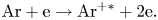
In low-temperature plasmas, metastable ions are often generated by a single ionization event with high-energy electrons (Chu, Hood & Skiff Reference Chu, Hood and Skiff2019). For example, in argon plasmas, this is expected to occur due to the following reaction:

(2.1)\begin{equation}\textrm{Ar} + \textrm{e} \to \textrm{A}{\textrm{r}^{ +{\ast} }} + 2\textrm{e}.\end{equation}

The signal intensity measured by LIF can be estimated by the CRM (Wilson et al. Reference Wilson, Finn, James and Falconer1995; Barnat & Weatherford Reference Barnat and Weatherford2015; Chu et al. Reference Chu, Mattingly, Berumen, Hood and Skiff2017; Chu & Skiff Reference Chu and Skiff2018), which estimates the generation and excitation rates of collision frequencies that produce metastable ions. These frequencies are given by the general collision model:

(2.2)\begin{equation}{S_{ij}} = {n_i}{n_e}\int_{ - \infty }^\infty {{\sigma _{ij}}(E){v_e}(E){f_e}(E)\,\textrm{d}E} = \; \langle {n_i}{n_e}{\sigma _{ij}}(E){v_e}(E)\rangle .\end{equation}

In this model, ${S_{ij}}$ denotes the rate at which the collision process excites ions or neutral particles from state i to state j, ${\sigma _{ij}}(E)$ and ${v_e}(E)$ are the energy distribution of the collisional cross-section and the electron velocity when transition at electron energy E, respectively, and ${f_e}(E)$ is the electron energy distribution. Through the collision model, the rate of metastable production can be estimated by the electron collision excitation process: $\langle {n_{meta}}{n_e}{\sigma _{excite}}(E){v_e}(E)\rangle$. Here ${n_{meta}}$, the density of metastable ions, can in turn be estimated by balancing the loss rate with the production rate: $\langle {n_{n,g}}{n_e}{\sigma _{nm}}(E){v_e}(E)\rangle \; + \langle {n_{i,g}}{n_e}{\sigma _{im}}(E){v_e}(E)\rangle$, each of these terms representing production of metastable ions from ground-state neutrals and ions by electron collisions.

The process of metastable excitation by a laser can be similarly treated as a photon–ion collision event, and the energy distribution of photons can be well approximated as a group of single-velocity particles incident at a photon flux ${\varGamma _{photon}}$. Thus the equation of this collision event can be simplified as ${n_i}{\sigma _{ij}}{\varGamma _{photon}}$ (Wilson et al. Reference Wilson, Finn, James and Falconer1995). Flux ${\varGamma _{photon}}$ can be determined by the laser injection power and wavelength.

According to this model, both laser photon collision excitation and electron collision excitation are summarized to obtain the rate at which metastable ions are excited to the excited state. In addition, metastable quenching rate ${S_{quench}}$ should also be included. Consequently, the excitation rate of the metastable ions given a metastable density ${n_{meta}}$ can be written as

(2.3)\begin{equation}{S_{ex}} = \; \langle {n_{meta}}{n_e}{\sigma _{excite}}(E){v_e}(E)\rangle \; + \; {n_{meta}}{\sigma _{LIF}}{\varGamma _{photon}}\; + \; {S_{quench}},\end{equation}

where $\langle {n_{meta}}{n_e}{\sigma _{excite}}(E){v_e}(E)\rangle$ is the electron collision excitation rate and ${S_{quench}} = \; \langle {n_{meta}}{n_n}{\sigma _{quench}}(E){v_i}(E)\rangle$ is the rate of collisional quenching caused by metastable collisions with background particles. Note that only a portion of the laser excitation rate ${n_{meta}}{\sigma _{LIF}}{\varGamma _{photon}}$ results in LIF signal, determined by the branching ratio of the transitions from the excited state to the different relaxed state.

The CRM is generally adapted to describe the physical processes behind plasma LIF diagnostics and could be considered a statistical model. Particularly with experiments employing continuous-wave lasers, this is at least in part due to the adaption of a low laser modulation frequency much lower than the fluorescence frequency, whether technologically limited or deliberately chosen by design (Wang & Hershkowitz Reference Wang and Hershkowitz2006; Yip et al. Reference Yip, Hershkowitz and Severn2010, Reference Yip, Hershkowitz, Severn and Baalrud2016). As the modulation frequency increases, the probabilistic aspect of the excitation process also becomes significant and will affect the resultant LIF signal. This work presents experimental investigation of such effects.

3. Probabilistic model and its effects on lock-in amplification

The fundamental physical model behind the CRM is that whether a photon excites a metastable is by nature probabilistic and the associated probability of excitation depends on the cross-section in question. The resultant photon count calculated from the CRM is therefore a statistically expected value. Provided a large number of events per observation, i.e. a sufficiently large number of photons streaming through a sufficient amount of metastables in the diagnosed space per modulated laser pulse, the resultant signal strength per pulse will be close to this expected value. However, as the number of expected excitation events per modulated pulse decreases, the number of probabilistic events within a pulse is no longer sufficient to form a statistical result. Rather, the total number of a large number of modulated pulses reflects the expected number of excitation events, i.e. fluorescent photons, per pulse. This transition from statistical to probabilistic signal can occur via metastable density, laser power and modulated pulse width reduction. The underlying mathematical process calculating the statistically and probabilistically expected signal strength is one and the same, but the probabilistic nature of this expected value is revealed as the number of events per pulse reduces. Thus, the physical picture of the CRM can be both statistical and probabilistic.

Here we revisit the working principles of lock-in amplification to examine how the microscopic probabilistic fluorescence affects signal retrieval. A phase-sensitive detector (PSD) is equivalent to a bandpass filter with extremely narrow bandwidth. The basic module includes a multiplication module for multiplying the input signal and the reference signal and a filter module effectively defining the integration time within which the multiplied signal is time-averaged.

Signal ${S_I}(t)$ is defined as a time–frequency input signal mixed with noise, and ${S_R}(t)$ is a reference signal with a fixed frequency relationship with the input signal to be measured. A signal with known modulation entering the PSD module can be defined as ${S_I}(t) = {A_I}\,\textrm{sin}(\omega t + \varphi ) + B(t)$, where $\omega$ is the modulation frequency and $B(t)$ is the total noise. The standard reference input to the signal channel is given as ${S_{R0}}(t) = {A_R}\,\textrm{sin}({\omega _0}t + \theta )$. After the two signals are input into the PSD module for multiplication at the same time, the output signal obtained is

(3.1)\begin{align}\begin{aligned} {S_{PSD0}} & = {S_I}(t){S_{R0}}(t) = {A_I}{A_R}\,\textrm{sin}(\omega t + \varphi )\,\textrm{sin}({\omega _0}t + \theta ) + B(t){A_R}\,\textrm{sin}({\omega _0}t + \theta )\\ & = 0.5{A_I}{A_R}\,\textrm{cos}[(\omega - {\omega _0})t + \varphi - \theta ] - 0.5{A_I}{A_R}\,\textrm{cos}[(\omega + {\omega _0})t + \varphi + \theta ]\\ & \quad + B(t){A_R}\,\textrm{sin}({\omega _0}t + \theta ). \end{aligned}\end{align}

When the test signal frequency and the reference frequency are not decoupled, it is usually assumed that $\omega = {\omega _0}$, that is, the frequencies of the reference signal and the modulated real signal are equal. At this time, the standard signal output by the reference signal channel is ${S_R}(t) = {A_R}\,\textrm{sin}(\omega t + \theta )$. Therefore, the output signal is ${S_{PSD0}} = {S_I}(t){S_R}(t) = \; 0.5{A_I}{A_R}\,\textrm{cos}(\varphi - \theta ) - 0.5{A_I}{A_R}$ $\textrm{cos}(2\omega + \varphi - \theta ) + B(t){A_R}\,\textrm{sin}(\omega t + \theta )$. If the modulated frequency of the input signal equals that of the reference signal, the amplitude of the signal to be measured, i.e. the intensity of the fluorescence signal in this experiment, can be extracted through the first item. The DC part can be obtained by passing the result into a low-pass filter, ${S_{output}} = \; 0.5{A_I}{A_R}\,\textrm{cos}(\varphi - \theta )$.

Figure 1(a,b) shows a schematic diagram of the event counts of metastable excitation and therefore fluorescence. The histogram is the total number of fluorescent photons that can be excited within the period of each pulse, which is a square wave with a duty cycle of 50 %. Ideally, the signal strength of each laser is equivalent to the excitation rate discussed in the previous section, giving constant real signal strength over each laser pulse. However, each laser excitation is in fact a probabilistic event. When the excitation frequency is much higher than the modulation frequency, the total photon collection count is essentially a manifestation of a macroscopic collection of excitation events, becoming very close to its statistically expected signal strength as described by the collisional excitation model. On the other hand, as we increase the modulation frequency and therefore reduce the temporal pulse width, the expected number of excitation events within a pulse reduces and eventually becomes totally probabilistic as the expected number of collected photons in each laser pulse becomes close to 1. That is, not every laser pulse produces a photon to be collected, and, within some, more than one photon will be collected. This probabilistic property of the microscopic fluorescence excitation process causes the real frequency of the fluorescent signal to be decoupled from the modulation frequency. Therefore, the output signal is treated by the PSD as noise and averages to 0. Fluorescent signal decoupled and eliminated by the PSD is represented as grey, and from figure 1(a) one can see that the fluorescent signal can be totally discarded by lock-in amplification. On the other hand, the transition from the macroscopic, statistically determined signal to the microscopic, probabilistic signal might not be a sharp one. There might exist a regime such that probabilistic effects manifest, but signal remains retrievable as the proportional variation total collectible photon count per laser pulse in most pulses remains within a relatively small range. This is illustrated in figure 1(b) using an expected photon count of 10 as an example. Due to the probabilistic nature of metastable excitation, not every laser pulse results in the expected photon count, but the proportion of random variation may not be so severe such that an $\omega = {\omega _0}$ baseline signal can still be strictly retrieved, although the random fluctuations are very likely to be discarded by lock-in amplification. As the modulation frequency decreases and pulse width increases, the collected photon count within a pulse converges to the statistically expected value, thus becoming almost totally retrievable by lock-in amplification. On the other hand, the collected photon count per laser pulse is not only limited by the fluorescence frequency but also by the solid angle which decides the proportion of excited photons being collected, and note that the direction of flight of each individual photon produced in an excitation event is also probabilistically determined.

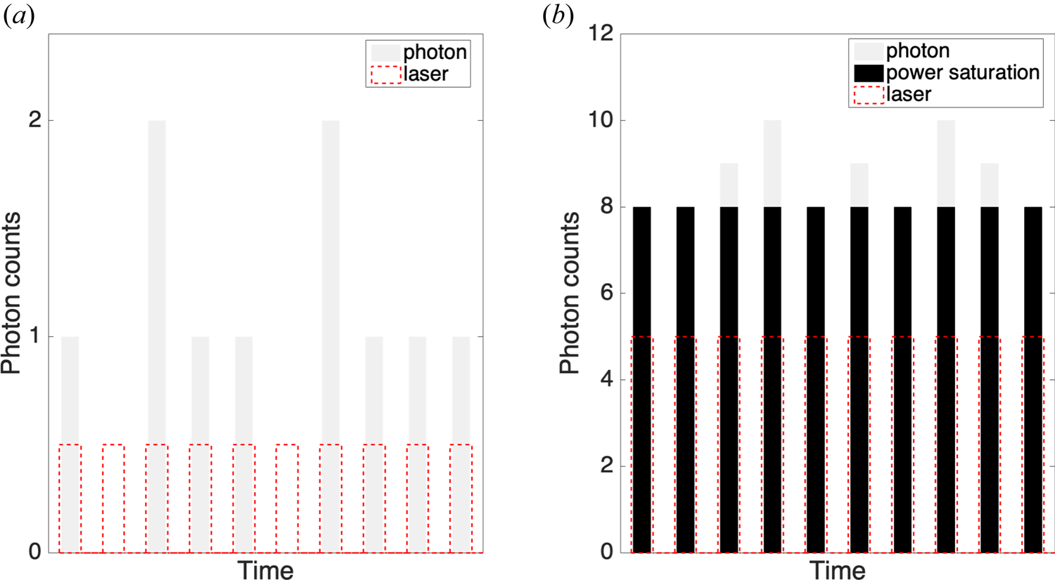
Figure 1. Schematic diagram of micro-process in which a metastable state can be excited to produce photons under laser input. (a) Single-photon case. (b) Multi-photon case.

4. Experimental set-up

Experiments are carried out in ASIPP's LIF Test Source (LTS), a multi-dipole confined hot cathode source. A schematic of LTS is shown in figure 2. The chamber is 40 cm long and 20 cm in diameter. Singly ionized argon plasma is produced by electron-impact ionization where primary electrons are emitted by a 2 mm diameter hot LaB₆ cathode. Multi-dipole confinement is realized by 16 rows of magnets with alternating polarities. These magnets are arranged around the periphery of the plasma. On the surface of the magnet, the magnetic field is 1600 G. In the measurement area, the magnetic field is rapidly reduced to less than 2 G. The cathode bias in this experiment is −140 V, which combines with the plasma potential V_p to give the primary electron energy. A mass flow controller is used to maintain a constant neutral gas inflow, thereby maintaining a constant neutral pressure in the chamber. The background pressure of the device is approximately 10⁻⁵ Pa, and the operating pressure ranges from 10⁻² to 10⁻¹ Pa. A Langmuir probe made with an 11 mm diameter tantalum disc is used to measure the electron density n_e and the electron temperature T_e. Typical plasma parameters for our experiments are T_e ~ 4 eV, n_e ~ 10⁹ cm⁻³.

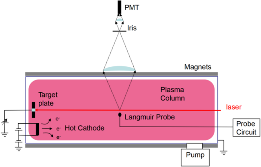
Figure 2. Schematic of the LTS multi-dipole chamber.

Our study adopted a three-level Ar II scheme in which a diode laser at a wavelength of 668.614 nm (in vacuum) excites the 3d ⁴F _7/2 argon ion metastable state to the 4p ⁴D _5/2 energy level, first proposed by Severn, Edrich & Mcwilliams (Reference Severn, Edrich and Mcwilliams1998). The fluorescence radiation from 4p ⁴D _5/2 to 4s ⁴P _3/2 has a wavelength of 442.72 nm (in vacuum). A schematic of the LIF optical set-up is shown in figure 3. The black solid lines and the black dotted lines represent the mirrors and laser beam splitters, respectively. A Wavicle ECDL 668 nm Littrow cavity diode laser is used, amplified with a Wavicle TA 668 nm tampered amplifier. The system has been configured to obtain a mode-hop-free tuning range of 100 GHz. In this study, only a small proportion of the tuning range is used, a tuning range of <15 GHz employed with a laser power change of less than 3 %. The laser is modulated via an acoustic optical modulator (AOM), which diffracts the beam periodically when a modulation is applied, splitting the laser beam. The modulation signal generated by the AOM is a square wave and the duty cycle is 50 %. The zeroth-order beam (the red solid line shown in figure 2), which was incompletely modulated, is directed into a set of wavelength/frequency measurements which are not modulation-sensitive. This beam is 1/10 split twice before being directed into an iodine cell enclosed in a ceramic housing (Keesee et al. Reference Keesee, Scime and Boivin2004; Severn, Lee & Hershkowitz Reference Severn, Lee and Hershkowitz2007) used for absolute wavelength calibration. A 1/10 split beam is directed into a Fabry–Pérot etalon with a free spectrum range of 1.5 GHz and a finesse of 200 (Cooper & Laurendeau Reference Cooper and Laurendeau1997). Another 1/10 split beam is directed into a HiFinesse WS-5 wavelength meter for online monitoring of mode-hop-free tuning. The first-order diffraction (the red dotted line shown in figure 2), which is completely modulated, is injected into the chamber through an optical fibre via optical fibre coupling, and then injected into the plasma. The Ar II fluorescent radiation is collected by a PMT at 90° relative to the axis of the laser beam shown in figure 1. The type of PMT is a Hamamatsu H19492-003 with a load resistance of 50 Ω. The control voltage is measured at 0.562 V and the gain is 10⁴. A SYSU OE 2031 DSP lock-in amplifier is used to recover the LIF signal from the ambient background noise. The laser scanning time is set to 10 s and the time constant is 30 ms. The recovered LIF signal is averaged over 32 scans. All data are collected using an oscilloscope.

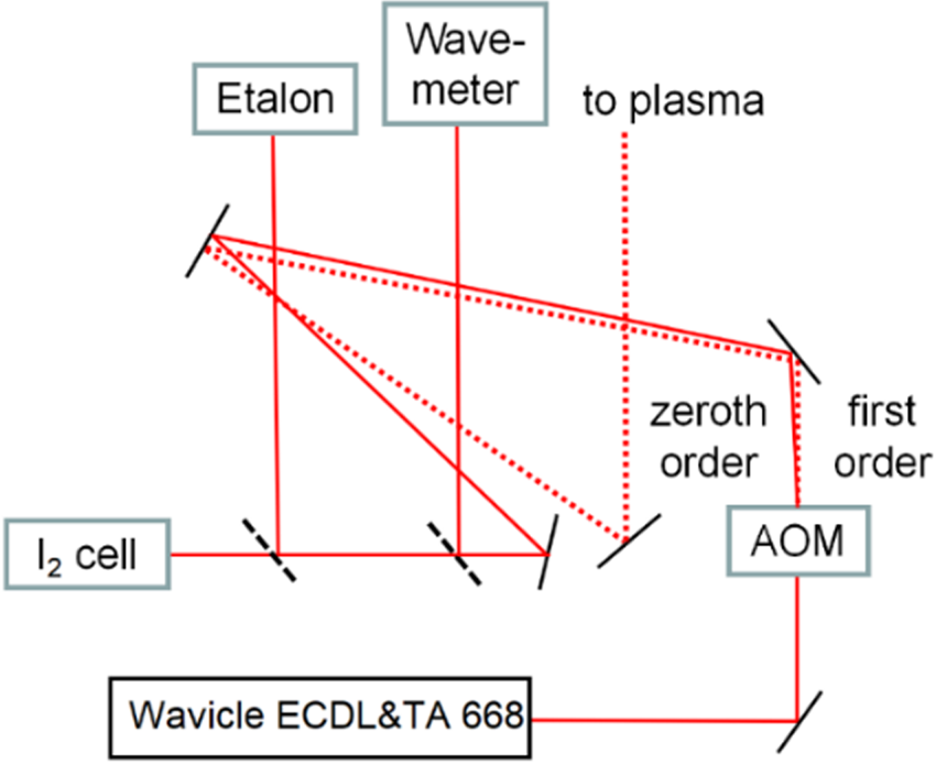
Figure 3. LIF experimental set-up.

5. Experimental results and discussion

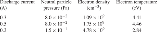
According to the collision model of metastable ion generation, fluorescence frequency can be changed by changing the production rate of metastable ions. This can in turn be done by, for example, changing the plasma discharge current or the neutral pressure, which changes the number of energetic electrons and neutrals from which metastable ions are produced. Two experiments of different discharge current are designed, as shown in figure 4. The electron temperature and electron density are measured by a Langmuir probe. The data are shown in table 1. The neutral pressure is controlled by the flowmeter and detected as 8.0 × 10⁻² Pa by the vacuum gauge. Figure 4(a) demonstrates that, for the same laser power injection, higher discharge currents result in higher fluorescence signals and their limit. In this work, all recorded signals are normalized by the sensitivity of the lock-in amplifier, and the sensitivity of the PMT stayed constant. Increasing the discharge current from 0.3 to 0.5 A gives an increased fluorescence signal by a factor of 1.46, which is significantly lower than the 1.67 ratio of discharge current increase. This may be due to the partial loss of the initial high-energy electrons produced by the hot cathode at low neutral pressure. Table 1 also shows that changing the discharge current does not significantly change T_e, but changing the neutral pressure does significantly change both n_e and T_e. This is expected as in a weakly ionized plasma, i.e. ${n_e} \ll {n_n}$, where n_n is the neutral density, energy dissipation of the energetic electrons is generally determined by electron loss to the wall and collisional loss to the background neutrals, both of which are relatively constant parameters with respect to discharge power unless a plasma is close to being fully ionized.

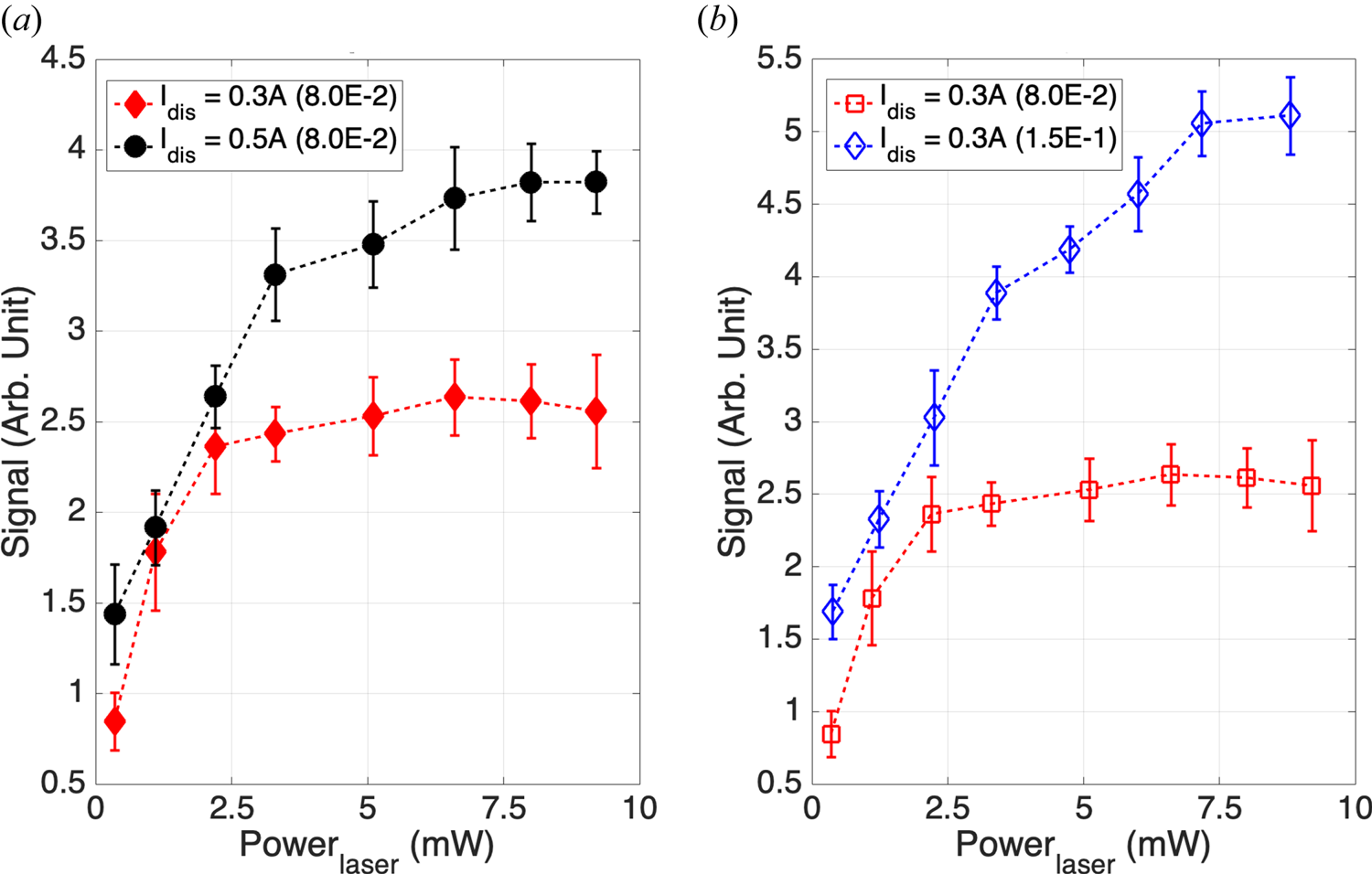
Figure 4. Changing laser power under different plasma discharge current (a) and different neutral pressure (b) to explore the output limit of fluorescence. The red diamond and the black circle represent discharge currents of 0.3 and 0.5 A, respectively (a). The blue diamond and red square represent the fluorescence signal intensity at neutral pressures of 1.5 × 10⁻¹ and 8.0 × 10⁻² Pa, respectively, while keeping the discharge current constant at 0.3 A (b).

Table 1. Electron temperature and electron density data measured by a Langmuir probe under three different conditions.

In the case of two different discharge currents, the intensity growth rate of fluorescence signal decreases with an increase of laser power. It can also be seen from figure 4(a) that at higher discharge current, the laser power needs to be higher to reach the fluorescence intensity limit. This is because a higher discharge current provides more energetic electrons, increasing the production rate of metastable ions.

The neutral pressure in the chamber can be accurately controlled by the gas flowmeter. Therefore, an experiment to study the generation limit of fluorescence signal under different neutral pressures was also designed. The experimental results are shown in figure 4(b). As shown, the proportional increase of LIF signal with an increase of neutral pressure is higher than that with an increase of discharge current. This is consistent with the results that a higher discharge current at a lower neutral pressure facilitates higher loss of primary electrons to the wall than to the collisions with neutral gas, and also consistent with results of previous studies that electron–neutral collisions produce both ground-state ions and metastable ions.

When the plasma parameters remain constant, the yield of metastable ions per unit time, i.e. the rate of metastable ion production, is limited. This in turn limits the excitation frequency of LIF for the same laser power. From figure 4, we can also obtain the laser power saturation under the three different conditions in table 1: 2.5 mW (0.3 A, 8.0 × 10⁻² Pa), 6.2 mW (0.5 A, 8.0 × 10⁻² Pa) and 7.5 mW (0.3 A, 1.5 × 10⁻¹ Pa), the parameters in parentheses representing discharge current and neutral particle pressure, respectively. Below we present results of exploring the frequency limit of fluorescence signal output, with the frequency modulation realized by AOM modulation of a continuous-wave laser.

The frequency limit of fluorescence output under changing discharge current and neutral pressure was also studied in this paper. In this series of experiments, the laser injection was kept unchanged at a low power (1.48 mW). It is worth noting that we used the function of automatic phase finding of the lock-in amplification before each experiment to avoid an excessive phase difference between the lock-in amplification and AOM, especially in the high-laser-chopping-frequency experiment, where the method of increasing the plasma discharge current and then accurately finding the phase is used. The results are shown in figure 5. The signal strength here indicates the integral value of the whole ion velocity distribution function signal strength under a Maxwell distribution to avoid the impact of noise signal on the peak value of the fluorescence signal. The effect of discharge current on fluorescence limit frequency is investigated first. The results are shown in figure 5(a). The four groups maintained the same neutral pressure and iris size. The fluorescence signal declines much more rapidly after the frequency with maximum signal is reached, as shown in figure 5(a), especially when the plasma discharge current is high. This is consistent with the collision excitation model for which an increased rate of primary electron injection increases the metastable production rate, which increases the fluorescence frequency. Before reaching the extreme value, the fluorescence signal intensity increases with an increase of laser input frequency, reflecting suppression of lower-frequency noise. The lower frequency mostly refers to the noise produced by the circuit. This noise has a broad spectrum of frequencies, and the frequency ranges could be composed of a Fourier expansion with the same frequency as the lock-in amplification. When the chopping frequency exceeds the broad-spectrum noise frequency ranges (which are often less than 200 kHz), this noise could be suppressed, resulting in an increase in signal strength. The shift to higher frequency with maximum signal strength at a higher discharge current and laser power indicates the association of such frequency with the fluorescence excitation frequency in the diagnosed volume, and that the background noise is broadband such that increasing modulation frequency removes an increasing portion of the frequency components of these noises. Once a maximum frequency is reached, the signal begins to decline with further increase of modulation frequency. It is worth noting that the decreasing amplitude of the signal will gradually decrease with a gradual increase of the chopper frequency. At the same time, this trend is also seen in the experiment of changing the neutral pressure in figure 5(b). With the modulated real signal not expected to be removed by lock-in amplification, this reduction of signal is therefore an evidence of frequency decoupling between the laser modulation and the waveform of the fluorescence signal.

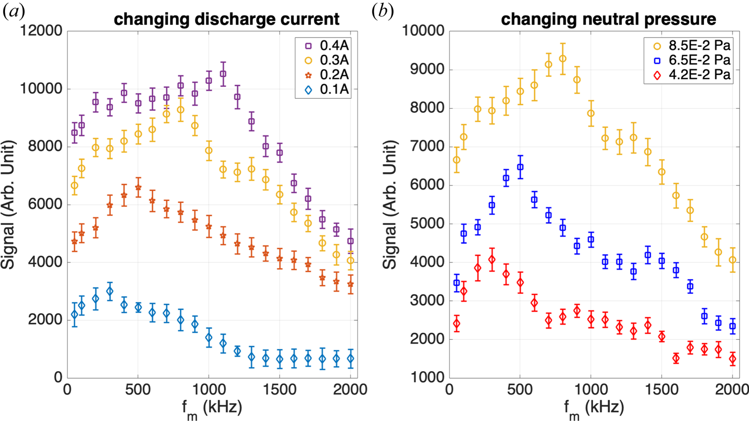
Figure 5. Exploring the frequency limit of fluorescence output under changing discharge current with the neutral pressure kept constant at 8.5 × 10⁻² Pa (a) and changing neutral pressure with a discharge current of 0.3 A (b).

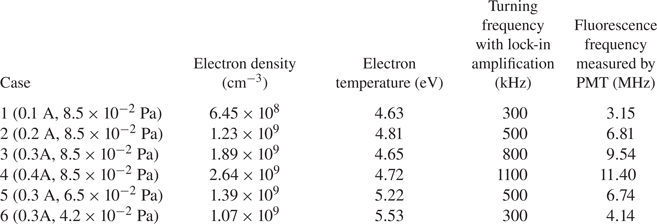
As listed in table 2, under these different sets of discharge parameters, several turning fluorescence frequencies were observed. Turning frequency here represents the extreme frequency observed experimentally. Meanwhile, the fluorescence frequency in table 2 represents the extreme frequency calculated by PMT gain. The fluorescence frequency can be calculated by converting the observed signal to the actual photon count via the PMT's luminous sensitivity. The PMT voltage signal is converted to light intensity in luminous units using the specified lumens-to-voltage sensitivity of the PMT provided by its manufacturer's test report, which is then converted to power units (watts) and thence the photon count using the photon energy of the fluorescent light calculated by E = hv. The calculated fluorescence frequencies are much higher than the turning frequency observed in the experiment. We believe that the optimal modulation frequency being at most 1/10 of the fluorescence frequency is specific to analogue lock-in amplification and is not generally applicable if signal amplification techniques are different. This is because the real frequency of the probabilistic signal becomes decoupled from the modulation frequency and analogue-based lock-in amplification is, obviously, particularly sensitive to the coupling of the reference frequency and the signal modulation frequency. On the other hand, the reduction of signal strength is found to be a very gradual process. This indicates the lack of a rapid transition from a statistically determined signal to a probabilistically determined signal, with which the whole signal should be removed by lock-in amplification. Rather, such a transition is a gradual process, with the total photon count per laser pulse becoming partially probabilistic, and lock-in amplification clips away the random ‘portion’ of the signal. That is, the gradual manifestation of the probabilistic nature of fluorescence photon counting is more like the case shown in figure 1(b) instead of a rapid transition to zero recovered signal, as with the case shown in figure 1(a). Note that the PMT is also not a single-photon detector, which might add to this effect. Therefore, this process needs to be considered when using the locked-in amplifier to extract the weak signal in the LIF experiment, and because the measured fluorescence signal generation frequency is far less than the theoretically calculated fluorescence frequency, this will bring restrictions in instability and other plasma high-frequency oscillation experiments.

Table 2. The turning frequency with lock-in amplification and the fluorescence frequency estimated by the photon count under the corresponding experimental conditions obtained by PMT gain conversion. (Case1: discharge current 0.1 A, 8.5 × 10⁻² Pa; case2: discharge current 0.2 A, 8.5 × 10⁻² Pa; case 3: discharge current 0.3 A, 8.5 × 10⁻² Pa; case 4: discharge current 0.4 A, 8.5 × 10⁻² Pa; case 5: discharge current 0.3 A, 6.5 × 10⁻² Pa; case 6: discharge current 0.3 A, 4.2 × 10⁻² Pa; all cases used the same laser power of 1.48 mW.) In addition, the electron temperature and density measured by a Langmuir probe are also shown.