


1. Introduction
Ongoing discussions (Shenkel et al. Reference Shenkel, Dorland, Baczewski, Boshier, Collins, Dubois, Houck, Humble, Loureiro and Monroe2018) on the potential of quantum information and computation in plasma physics have recently led to exploiting Hilbert-space approaches in the numerical simulation of magnetized plasmas (Dodin & Startsev Reference Dodin and Startsev2020; Engel, Smith & Parker Reference Engel, Smith and Parker2019, Reference Engel, Smith and Parker2021; Joseph Reference Joseph2020), of the Navier–Stokes equations (Gaitan Reference Gaitan2020), and of arbitrary non-Hamiltonian systems of equations (Joseph Reference Joseph2020; Liu et al. Reference Liu, Kolden, Krovi, Loureiro, Trivisa and Childs2020). In particular, recent work (Joseph Reference Joseph2020) has emphasized the role of Koopman wavefunctions in classical dynamics while their usage in describing hybrid quantum-classical systems was presented in Bondar, Gay-Balmaz & Tronci (Reference Bondar, Gay-Balmaz and Tronci2019), Boucher & Traschen (Reference Boucher and Traschen1988), Gay-Balmaz & Tronci (Reference Gay-Balmaz and Tronci2019), Tronci & Gay-Balmaz (Reference Tronci and Gay-Balmaz2021), Sudarshan (Reference Sudarshan1976) and Jauslin & Sugny (Reference Jauslin and Sugny2010). In this paper, we want to show how these enter in the variational and Hamiltonian formulation of Vlasov kinetic theory.
In the context of the classical Liouville equation $\partial _t\,f=\{H,f\}$ , the idea of a Koopman wavefunction emerges naturally from the fact that the phase-space density is positive–definite, so that the relation $f(x,p)=|\varPsi (x,p)|^2$
 induces a Hilbert-space description of classical mechanics hinging on the Koopman–von Neumann (KvN) equation (Koopman Reference Koopman1931; von Neumann Reference von Neumann1932; Mauro Reference Mauro2002)

and $\{\cdot ,\cdot \}$ denotes the canonical Poisson bracket. Here, the Liouvillian operator $\hat {L}_H$
 associated to the Hamiltonian H is self-adjoint so that the Koopman wavefunction undergoes a unitary dynamics, thereby leading to a quantum analogy. While the Koopman propagator $\exp (-\textrm {i}\hbar ^{-1}\hat {L}_H)$
 (Koopman operator) often appears in the dynamical systems literature (Budišić, Mohr & Mezić Reference Budišić, Mohr and Mezić2012; Giannakis et al. Reference Giannakis, Ourmazd, Slawinska and Schumacher2020), the role of Koopman wavefunctions is being recognized in physics only recently. Over the decades, prominent authors such as Berry (Reference Berry1992), Chirikov, Izrailev & Shepelyanskii (Reference Chirikov, Izrailev and Shepelyanskii1988), Della Riccia & Wiener (Reference Della Riccia and Wiener1966) and ’t Hooft (Reference ’t Hooft1997) have discussed Koopman wavefunctions without referring to Koopman's original work. However, the interest in Koopman wavefunctions has been recently revived by their role in the quantum-classical divide (Bondar et al. Reference Bondar, Cabrera, Lompay, Ivanov and Rabitz2012).
One of the important motivations for the introduction of the Koopman formalism is to develop a rigorous Hilbert-space theory for the approximation of the particle distribution function (PDF). For example, it is well known that the linearized Vlasov–Maxwell equation possesses Case–van Kampen eigenmodes and one might wish to understand how an expansion in eigenmodes, or some other complete set of eigenfunctions, converges to a solution of the nonlinear Vlasov–Maxwell equations. This point of view was taken by Koopman and von Neumann in their development of ergodic theory.
Yet another important application of the Koopman approach is the development of quantum algorithms for simulating nonlinear classical dynamical systems (Joseph Reference Joseph2020). In principle, quantum computers can store and process an exponentially large amount of information efficiently and can perform certain calculations, such as the ‘quantum’ Fourier transform, very efficiently (Nielsen & Chuang Reference Nielsen and Chuang2010). While quantum computers hold great promise, they can only perform linear unitary operations on normalized wavefunctions. A number of authors, such as Alanson (Reference Alanson1992), Chirikov et al. (Reference Chirikov, Izrailev and Shepelyanskii1988) and Joseph (Reference Joseph2020), have reformulated nonlinear non-Hamiltonian dynamics as a linear unitary evolution of functions on phase space. Thus, as shown in Joseph (Reference Joseph2020), quantum Hamiltonian simulation algorithms for the Koopman evolution operator can achieve up to an exponential speedup over an Eulerian discretization of the PDF and using amplitude estimation of physical observables leads to up to a quadratic speedup over Lagrangian discretizations based on Monte Carlo and particle-in-cell.
Depending on the choice of phase, Koopman wavefunctions are related to the Clebsch representation of the Vlasov distribution (Morrison Reference Morrison1981), which may be of more common knowledge in the plasma physics community. However, as discussed in § 2.1, the complete identification between Koopman wavefunctions and Clebsch variables may require the Koopman phase to be singular at some points or regions in phase space (Joseph Reference Joseph2020). In turn, the phase is irrelevant in the KvN theory and one should be able to set it to zero without affecting the general formulation of the theory. In order to overcome this possible issue, we develop an alternative non-canonical formulation that indeed allows for a zero phase. As shown in § 2.2, this formulation follows from a suitable adaptation of the Euler–Poincaré variational principle for the standard Vlasov dynamics (Cendra et al. Reference Cendra, Holm, Hoyle and Marsden1998; Squire et al. Reference Squire, Qin, Tang and Chandre2013; Tronci Reference Tronci2013). In this case, the relation to standard Clebsch variables is replaced by a momentum map structure that is discussed in § 2.3. Then, § 2.4 applies this construction to the Vlasov–Maxwell system.
In addition, a variant of the KvN construction called the ‘Koopman–van Hove equation’ (KvH) will also be illustrated in § 3. As shown in § 3.1, in this variant the KvN equation emerges as the amplitude equation, while the evolution of the phase is given by the classical action, i.e. the integral of the Lagrangian function, following Feynman's general prescription. The KvH formulation is based on a slight extension of standard canonical transformations that first appeared in van Hove's thesis (van Hove Reference van Hove1951) and is briefly discussed in § 3.2. As the KvH construction is based on a canonical Hamiltonian structure, its relation to the Vlasov density comprises an extension of the standard Clebsch representation, as presented in § 3.3. Then, § 3.4 couples the KvH equation to the evolution of the electromagnetic fields and presents the resulting Hamiltonian structure. Finally, § 3.5 discusses the role of gauge transformations in the KvH context.
2. Koopman-von Neumann theory
In this section, we present two alternative formulations of the KvN theory. The first formulation is canonical. In this case, the Hamiltonian functional depends on the phase and vanishes if the latter is initially set to zero. Indeed, this Hamiltonian generally differs from the expression of the total energy obtained by Koopman's prescription $f=\left |\varPsi \right |^2$ . This ambiguity may be overcome by enforcing a specific constraint on the phase (Joseph Reference Joseph2020) thereby leading to branch-cut singularities. We show that these intricacies can be removed by resorting to an alternative non-canonical formulation that is entirely built upon the prescription $f=\left |\varPsi \right |^2$
 , so that the Hamiltonian functional is independent of the phase which can then be set to zero. In order to simplify the notation, most of our discussion will treat the case of a single degree of freedom, so that the phase space is two-dimensional. The generalization to multiple degrees of freedom is straightforward, and will be used when discussing the Vlasov–Maxwell system.
2.1. Clebsch variables and canonical structure
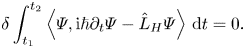
As first discussed in Dodin (Reference Dodin2014), the KvN equation is Hamiltonian with the canonical Hamiltonian structure arising from the following Dirac–Frenkel variational principle (Frenkel Reference Frenkel1934)
Here, $\varPsi$ is a square-integrable complex function, $\langle A,B\rangle =\operatorname {Re}\langle A|B\rangle$
 is the real-valued pairing associated with the standard $L^2$
 inner product $\langle A|B\rangle =\int A(x,p)^* B(x,p)\,\textrm {d} x\,\textrm {d} p$
 , and we have $\operatorname {Im}\langle A|B\rangle =\langle \textrm {i}A,B\rangle$
 . As discussed in Bondar et al. (Reference Bondar, Gay-Balmaz and Tronci2019) and Joseph (Reference Joseph2020), this Hamiltonian structure readily identifies a Hamiltonian functional given by

This is accompanied by the usual Poisson bracket from standard quantum mechanics (Chernoff & Marsden Reference Chernoff and Marsden1976; Foskett, Holm & Tronci Reference Foskett, Holm and Tronci2019)

where we have introduced the double-bracket notation $\{\!\{\cdot ,\cdot \}\!\}$ to distinguish from the canonical Poisson bracket. Then, the Madelung transform $\varPsi =\sqrt {D}\textrm {e}^{\textrm {i}S/\hbar }$
 expresses the Koopman wavefunction in terms of the density $D$
 and the phase $S$
 , thereby leading to the celebrated Clebsch representation of the real-valued Vlasov density (Holm & Kupershmidt Reference Holm and Kupershmidt1983; Marsden & Weinstein Reference Marsden and Weinstein1983; Morrison Reference Morrison1981), that is
Here, the classical Liouville equation $\partial _t\,f=\{H,f\}$ follows by combining the Jacobi identity with the relations

which arise from (1.1). For example, this formulation appeared in Neiss (Reference Neiss2019), where the Clebsch representation was used together with Koopman's original prescription $f=|\varPsi |^2$ in the context of the Vlasov–Poisson system for electrostatic plasmas. In symplectic geometry, the map $\varPsi \mapsto \hbar \operatorname {Im}\{\varPsi ^*,\varPsi \}$
 identifies a momentum map for the action of canonical transformations on the Hilbert space $\mathcal {H}$
 of Koopman wavefunctions, which is endowed with the canonical Poisson structure in (2.3). See § 2.3 later on for the definition of momentum maps.
This picture leads us to two following important observations. First, the relation (2.4) differs from Koopman's prescription $f=|\varPsi |^2$ for the phase-space density. Second, the Clebsch representation (2.4) does not generally identify a probability density, since $\int \{D,S\}\,\textrm {d} x\,\textrm {d} p=0$
 whenever $D$
 and $S$
 are differentiable continuous functions. In Joseph (Reference Joseph2020), a solution to this apparent issue was provided by selecting a singular phase ensuring the following consistency condition

Due to the equations of motion (2.5a,b), if this relation holds true as an initial condition, then it will hold for all time. In this case, the expression of the phase is necessarily singular and this is strictly necessary to produce the boundary terms generally required for the Clebsch representation (2.4) to hold true. Then, in this context, we realize that the KvN construction may be envisioned as a special case of Clebsch representation of the Vlasov density (Joseph Reference Joseph2020).
Notice that this representation requires a non-vanishing phase, which again contrasts with the phase invariance of the original prescription $f=|\varPsi |^2$ . Indeed, while one might wish to set the phase to zero and identify the Koopman wavefunction with a real-valued amplitude, this possibility is excluded by the Clebsch representation, which requires a non-zero phase by construction.
Whether or not the requirement of a non-zero, possibly singular phase is regarded as an issue, it may still be desirable to develop a Hamiltonian structure of KvN theory that does not necessitate the presence of a non-trivial phase. In view of this, we will proceed by considering an alternative non-canonical Hamiltonian structure of KvN theory, which appears to overcome this potential ambiguity.
Remark 2.1 (Guillemin–Sternberg collectivization) We remark that, in both the canonical and the non-canonical cases, Koopman wavefunctions provide a representation of the Liouville (Vlasov) density whose dynamics is then governed by the usual Lie–Poisson bracket on the Poisson algebra of phase-space functions (Marsden & Weinstein Reference Marsden and Weinstein1981/82; Marsden et al. Reference Marsden, Weinstein, Ratiu, Schimd and Spencer1983; Morrison Reference Morrison1986). The procedure taking the Koopman Hamiltonian structure into the Vlasov Lie–Poisson structure is an example of collectivization by a momentum map (Guillemin & Sternberg Reference Guillemin and Sternberg1980), which serves as the unifying geometric framework in this work; see § 2.3. Specifically, the canonical action of a Lie group on a Poisson manifold induces a momentum map generalizing Noether's conserved quantity occurring in the particular case of a symmetry group. Then, when a Hamiltonian function(al) can be entirely written in terms of this momentum map, the Hamiltonian is called ‘collective’, borrowing the terminology from nuclear physics (Guillemin & Sternberg Reference Guillemin and Sternberg1980). Here, we derive collective Hamiltonians for a series of models in Vlasov dynamics for which the Lie group is given by canonical transformations (or variants thereof, as in § 3.2). In this process, different Clebsch-type representations emerge from different actions on the Hilbert space of Koopman wavefunctions. Alternatively, depending on convenience, one may prefer to keep working with the Vlasov density itself.
2.2. Euler–Poincaré variational formulation
In this section, we shall start by presenting the Euler–Poincaré formulation of KvN theory. We start from the Euler–Poincaré variational principle for the classical Liouville equation
As discussed extensively in Cendra et al. (Reference Cendra, Holm, Hoyle and Marsden1998), Squire et al. (Reference Squire, Qin, Tang and Chandre2013) and Tronci (Reference Tronci2013), this variational principle arises from a symmetry reduction from the Lagrangian-path formulation in phase space to the corresponding Eulerian-variable description. Indeed, if we introduce the notation $\Bbb {J}^{j\ell }=\{z^j,z^{\ell }\}$ and ${\boldsymbol {z}}_0=(x_0,p_0)$
 is the phase-space label coordinate, then the equation of motion $\dot {\boldsymbol \eta }=\Bbb {J}\boldsymbol {\nabla } H(\boldsymbol \eta )$
 of the Lagrangian trajectory $\boldsymbol \eta ({\boldsymbol {z}}_0,t)=(\eta _q({\boldsymbol {z}}_0,t),\eta _p({\boldsymbol {z}}_0,t))$
 follows from the variational principle $\delta \int _{t_1}^{t_2}\int f_0(\eta _p\dot {\eta }_q-H(\eta _q,\eta _p))\,\textrm {d} x_0\,\textrm {d} p_0\,\textrm {d} t=0$
 , where $f_0({\boldsymbol {z}}_0)$
 is the reference density. In turn, the latter variational principle leads to the Eulerian counterpart (2.7) by a mere change of variables. Upon denoting by ${\boldsymbol {z}}=(x,p)$
 the Eulerian phase-space coordinate, the Eulerian phase-space density evolves according to the Lagrange-to-Euler map

Here, $\det \boldsymbol {\nabla }\boldsymbol \eta$ denotes the Jacobian determinant. In addition, we define the Eulerian phase-space vector field ${\boldsymbol {X}}=(u,\sigma )$
 such that

In this setting, we also define the infinitesimal displacement ${\boldsymbol \varXi }({\boldsymbol {z}},t)=\delta {\boldsymbol \eta }({\boldsymbol {z}}_0,t)|_{{\boldsymbol {z}}_0=\boldsymbol \eta ^{-1}({\boldsymbol {z}},t)}$ so that the Euler–Poincaré variations read

which are obtained from the defining relations (2.8) and (2.9). Here, $\boldsymbol \varXi$ is an arbitrary displacement vanishing at the endpoints, i.e. $\boldsymbol \varXi (t_1)=\boldsymbol \varXi (t_2)=0$
 . Then, the Euler–Poincaré variational principle (2.7) yields ${\boldsymbol {X}}=\Bbb {J}\boldsymbol {\nabla } H$
 , which is accompanied by the continuity equation $\partial _t\,f+{\operatorname {div}(\,f{\boldsymbol {X}})=0}$
 following from (2.8), thereby returning $\partial _t\,f+\{f,H\}=0$
 .
.
The Euler–Poincaré approach for the KvN theory arises immediately from the construction above. Indeed, the Koopman description $f=|\varPsi |^2$ immediately leads to

which is the standard Lagrange-to-Euler map for half-densities (Bates & Weinstein Reference Bates and Weinstein1997). This evolution law leads to the relations

One can introduce the operators $\hat {\varLambda }_\ell =-\textrm {i}\hbar \partial _\ell$ to write the above as Schrödinger-like equations

where $[\cdot ,\cdot ]_+$ denotes the anticommutator, $\hat {X}^\ell$
 are simply the multiplicative operators identified by the components of ${\boldsymbol {X}}$
 and likewise for $\hat {\varXi }^\ell$
 . Notice that here we are not asking for the vector field ${\boldsymbol {X}}$
 to be Hamiltonian: as we shall see, this property will result as a consequence of the variational principle under consideration. In more generality, the evolution law (2.11) and its equation of motion in (2.12a,b) also appear in other contexts involving non-Hamiltonian dynamical systems (Alanson Reference Alanson1992; Joseph Reference Joseph2020).
Since we are interested in the Hamiltonian structure, we shall write the Euler–Poincaré variational principle in terms of an arbitrary Hamiltonian functional $h(\varPsi )$ as follows:
where we recall (2.9). Here, the arbitrary functional $h(\varPsi )$ generally depends on $\varPsi$
 and its conjugate $\varPsi ^*$
 . Upon combining (2.12a,b) with the first equation in (2.10a,b), the Euler–Poincaré variational principle yields

Here, we have used the functional derivative notation so that $\delta h:=\langle {\delta h}/{\delta \varPsi },\delta \varPsi \rangle$ and, following Holm, Marsden & Ratiu (Reference Holm, Marsden and Ratiu1998), we have defined the diamond operator $\diamond$
 for compactness of notation.
Then, the wavefunction equation for an arbitrary Hamiltonian is obtained by substituting (2.15a,b) in the first equation of (2.12a,b), which leads to quite a cumbersome explicit form. However, in the case of KvN theory, this simplifies substantially. Indeed, if the Hamiltonian functional depends only on $f=|\varPsi |^2$ , then the chain rule relation ${\delta h}/{\delta \varPsi }={2}({\delta h}/{\delta f})\varPsi$
 transforms (2.15a,b) to the Hamiltonian vector field

thereby recovering the KvN equation (1.1) in the general form

In this case, the Lagrangian trajectory is a canonical transformation so that the propagator (2.11) reduces to $\varPsi ({\boldsymbol {z}},t)=\varPsi _0({\boldsymbol {z}}_0)|_{{\boldsymbol {z}}_0={\boldsymbol \eta }^{-1}({\boldsymbol {z}},t)}$ .
.
Notice that, while here we have used canonical coordinates associated with the canonical symplectic form $\textrm {d} x\wedge \textrm {d} p$ , the possibility of a non-canonical structure does not pose any difficulty. Indeed, one would simply redefine canonical transformations as symplectomorphisms, that is smooth invertible transformations preserving the non-canonical symplectic structure. Then, the Liouvillian operator $\hat {L}_H=\{\textrm {i}\hbar H,\, \}$
 would naturally involve the corresponding non-canonical Poisson bracket.
2.3. Non-canonical Poisson bracket and momentum map structure
We realize that (2.17) arises naturally from the Euler–Poincaré formulation of the Liouville equation, while its underlying structure is quite involved and this reflects in an intricate non-canonical Hamiltonian structure. Given an arbitrary functional $k(\varPsi )$ , the usual relation $\dot {k}=\{\!\{k,h\}\!\}$
 leads in this case to

which reduces to the Lie–Poisson bracket
in the case of functionals depending only on $f=|\varPsi |^2$ . To obtain (2.18), we have used the relation $\langle {\varPsi \diamond \varUpsilon },{\boldsymbol W}\rangle =\langle \varUpsilon ,{\boldsymbol W}\cdot \boldsymbol {\nabla }\varPsi +\operatorname {div}({\boldsymbol W})\varPsi /2\rangle$
 for any Koopman wavefunctions $\varPsi$
 and $\varUpsilon$
 , and any vector field ${\boldsymbol W}$
 . Indeed, this relation leads to

where the last equality follows from (2.15a,b). While expanding the terms in (2.18) does not lead to much insight, the present formulation has the advantage of restoring the use of the relation $f=|\varPsi |^2$ everywhere in the problem. For example, the standard expression of the total energy now coincides unambiguously with the Hamiltonian functional, which no longer vanishes upon setting the phase to zero.
We conclude this section by showing that the map $\varPsi \mapsto |\varPsi |^2$ is a momentum map (Marsden & Ratiu Reference Marsden and Ratiu1998) associated with the following (left) group action of canonical transformations: $\varPsi \mapsto \varPsi \circ {\boldsymbol \eta }^{-1}$
 , where $\circ$
 denotes composition of functions. By the arguments in Remark 2.1, this ensures that the Poisson bracket (2.18) consistently reduces to (2.19) for any two functionals $k$
 and $h$
 of the type $k(\varPsi )=\tilde {k}(|\varPsi |^2)$
 . Given the canonical action of a Lie group $G$
 on a manifold $M$
 with Poisson structure $\{\!\{\cdot ,\cdot \}\!\}$
 , a momentum map ${\mathcal {J}}:M\to \mathfrak {g}^*$
 is defined as

for any function $k$ on $M$
 and any element $\xi$
 of the Lie algebra $\mathfrak {g}$
 of $G$
 . Here, $\mathfrak {g}^*$
 denotes the dual space of $\mathfrak {g}$
 , $\langle \cdot ,\cdot \rangle$
 is the duality pairing, $\textrm {d}$
 is the differential on $M$
 and $\xi _M$
 denotes the infinitesimal generator of the $G$
 -action on $M$
 . If $G$
 is a symmetry of the Hamiltonian, then ${\mathcal {J}}(x)$
 is conserved in time by Noether's theorem. The Lie algebra of the group of canonical transformations is the space of Hamiltonian vector fields ${\boldsymbol {X}}={\boldsymbol {X}}_\xi$
 , where $\xi =\xi (x,p)$
 is a scalar function. Up to the addition of irrelevant constants, this space can be identified with the space of phase-space functions endowed with the canonical Poisson bracket. Then, the corresponding infinitesimal action on the Koopman Hilbert space $\mathcal {H}=L^2(\Bbb {R}^2)$
 is given by $\xi _{\mathcal {H}}(\varPsi )=-{\boldsymbol {X}}_\xi \cdot \boldsymbol {\nabla }\varPsi =\{\xi ,\varPsi \}$
 . Upon using the $L^2$
 -pairing, we compute

so that

thereby proving (2.21). This picture extends the usual Clebsch representation treated in § 2.1 to the non-canonical case. By proceeding analogously, one proves that the quantities

comprise the plasma-to-fluid momentum map (Marsden et al. Reference Marsden, Weinstein, Ratiu, Schimd and Spencer1983). Specifically, these are momentum maps for the action of momentum translations $(x,p)\mapsto (x,p-\textrm {d} \varphi (x))$ and configuration-space diffeomorphisms $(x,p)\mapsto (\eta (x),-p\,\textrm {d}\eta (x))$
 , respectively.
2.4. The KvN–Maxwell system
In this section, we want to apply the previous non-canonical formulation to the Maxwell–Vlasov system of magnetized plasmas. The canonical treatment is found in Neiss (Reference Neiss2019) for the case of the electrostatic limit. In the full electromagnetic case, gauge invariance naturally acquires a prominent role. In particular, the gauge freedom manifests itself in the Lagrangian formulation of Maxwell's equations through the fact that the Lagrangian is independent of $\partial _t \varPhi$ , and, hence, variations with respect to $\varPhi$
 serve to enforce Gauss’ law as a constraint. In the absence of sources, the Maxwell Lagrangian is written as

where
is the Maxwell Hamiltonian expressed in terms of the standard $L^2$ -norm. If we express the Vlasov density in non-canonical coordinates, we can construct the variational principle by an immediate extension of (2.14). We write

where

is the Hamiltonian, while Gauss’ law is enforced in (2.27) by the Lagrange multiplier $\varPhi$ . Using (2.12a,b) and the first equation in (2.10a,b), we obtain

In addition, arbitrary variations of the fields lead to

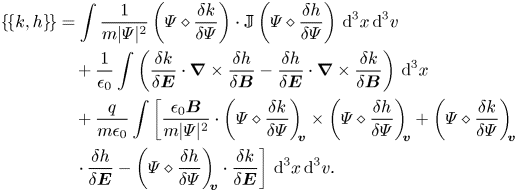
Here, the subscript ${\boldsymbol {v}}$ denotes the velocity components of vector-valued quantities in phase space. These equations reveal an intricate Hamiltonian structure whose Poisson bracket can be easily obtained by applying the usual relation $\dot {k}=\{\!\{k,h\}\!\}$
 upon expanding $\dot {k}=\langle \delta k/\delta \varPsi ,\partial _t\varPsi \rangle +\langle \delta k/\delta {\boldsymbol {E}},\partial _t{\boldsymbol {E}}\rangle +\langle \delta k/\delta {\boldsymbol {B}},\partial _t{\boldsymbol {B}}\rangle$
 and using the equations of motion for an arbitrary gauge-invariant Hamiltonian $h$
 . Indeed, upon taking the curl of the first equation in (2.30a,b) and using $\delta h/\delta {\boldsymbol {A}}=\boldsymbol {\nabla }\times \delta h/\delta {\boldsymbol {B}}$
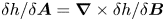 , one obtains the following structure:
Then, one can simply evaluate

so that $\mathbb {J} (\varPsi \diamond {\delta h}/{\delta \varPsi })=(m{\boldsymbol {v}},0)\left |\varPsi \right |^2$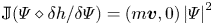 . Introducing the notation ${\hat {\boldsymbol {\varLambda }}=-\textrm {i}\hbar (\boldsymbol {\nabla }_{{\boldsymbol {x}}},\boldsymbol {\nabla }_{{\boldsymbol {v}}})}=({{\boldsymbol \lambda }}_{{\boldsymbol {x}}},{{\boldsymbol \lambda }}_{{\boldsymbol {v}}})$
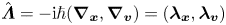 , the KvN equation reads

which is accompanied by Faraday and Ampére's law

Here, the first equation is obtained by taking the curl of the first equation in (2.30a,b).
3. Koopman-van Hove theory
As we saw in previous sections, the KvN phase remains constant along the phase-space Lagrangian trajectories; see the second equation in (2.5a,b). Indeed, in the KvN construction the phase is entirely irrelevant and plays the role of a gauge freedom in the relation $f=|\varPsi |^2$ . However, in classical mechanics one usually relates the classical phase to the Lagrangian function. Specifically, in Hamilton–Jacobi theory the phase is a function in configuration space and this function is given by the classical action integral. We observe that this is different from the Koopman phase, which instead is defined on phase space. As we shall see, the KvH construction combines the theory of Koopman wavefunctions with Feynman's prescription of a phase expressed in terms of the Lagrangian. Again, to keep the notation as simple as possible, the phase space will be two-dimensional in most of our discussion. The extension to six dimensions is straightforward and will be used when coupling the KvH equation to the electromagnetic fields.
3.1. The KvH equation
An alternative theory of classical mechanics based on Koopman wavefunctions goes back to van Hove's thesis (van Hove Reference van Hove1951), where canonical transformations were extended to include phase factors. As later shown by Kostant (Reference Kostant1970), in this setting the phase function is again identified with the action integral, which is now defined in terms of the phase-space Lagrangian. In this setting, the KvN equation (1.1) becomes the KvH equation

Here, $\hat {L}_H=\partial _xH{\lambda }_p-\partial _pH{\lambda }_x$ while $\mathscr {L}$
 is the expression of the phase-space Lagrangian, which now identifies a phase term. The information contained in this equation may be unfolded by applying the Madelung transform $\varPsi =\sqrt {D}\textrm {e}^{\textrm {i}S/\hbar }$
 , which leads to

The second equation can be formally solved in terms of the Lagrangian trajectories as (Gay-Balmaz & Tronci Reference Gay-Balmaz and Tronci2019, Reference Gay-Balmaz and Tronci2021)

thereby showing how the phase evolution emerges from the integral of the Lagrangian, in analogy to Feynman's path-integral formulation of quantum mechanics. For a discussion of the relation between equation (3.3) and the Hamilton–Jacobi equation, see de Gosson's work in de Gosson (Reference de Gosson2004).
Remark 3.1 (Relation to hybrid quantum-classical dynamics) Notice that, for Hamiltonians of the type $H=T+V$ , enforcing $\partial _p\varPsi =0$
 and replacing $p\to -\textrm {i}\hbar \partial _x$
 takes (3.1) into the quantum Schrödinger equation, thereby justifying the early name ‘prequantum Schrödinger equation’ (Kostant Reference Kostant1970). Indeed, (3.1) first appeared within the context of prequantization theory (Kirillov Reference Kirillov2001; van Hove Reference van Hove1951) and it has remained pretty unknown over the decades. Recently, it was recognized how this equation may actually lead to a consistent theory of quantum-classical coupling (Bondar et al. Reference Bondar, Gay-Balmaz and Tronci2019; Gay-Balmaz & Tronci Reference Gay-Balmaz and Tronci2019; Tronci & Gay-Balmaz Reference Tronci and Gay-Balmaz2021), where the phase plays a crucial role. Partly inspired by Kirillov (Reference Kirillov2001), the authors of Bondar et al. (Reference Bondar, Gay-Balmaz and Tronci2019) and Gay-Balmaz & Tronci (Reference Gay-Balmaz and Tronci2019) called (3.1) the ‘Koopman–van Hove equation’ in recognition of the very first contributions from Koopman and van Hove.
3.2. Geometric setting
While canonical transformations are enough to characterize the evolution of Koopman wavefunctions in KvN theory, the presence of the phase in the KvH formalism requires extending the KvN picture. A more detailed summary of the geometric setting of KvH theory is found in Faure (Reference Faure2007), Gay-Balmaz & Tronci (Reference Gay-Balmaz and Tronci2019) and Gay-Balmaz & Tronci (Reference Gay-Balmaz and Tronci2021). First, one introduces the $U(1)$ -bundle $\Bbb {R}^{2}\times U(1)$
 , where $\Bbb {R}^{2}$
 is the Euclidean two-dimensional phase space and $U(1)$
 is the group of complex phase factors. Gauge transformations are identified, as usual, with local phase factors so that the KvH wavefunction evolves according to compositions of gauge transformations and canonical transformations, that is

Notice that, unlike (2.11), here we are restricting the Lagrangian trajectory to identify a canonical transformation at all times. The geometric characterization of the phase factor in (3.4) needs further discussion. Specifically, the relation between the phase factor and the phase-space Lagrangian emerges as follows. Upon defining the gauge connection $\boldsymbol {\mathcal {A}}=p \,\textrm {d} x$ , it is well known (Marsden & Ratiu Reference Marsden and Ratiu1998) that $\textrm {d}(\eta ^*\boldsymbol {\mathcal {A}}-\boldsymbol {\mathcal {A}})=0$
 , where $\textrm {d}$
 is the exterior differential and $\eta ^*\boldsymbol {\mathcal {A}}({\boldsymbol {z}}):={\mathcal {A}}_\ell (\boldsymbol \eta ({\boldsymbol {z}}))\boldsymbol {\nabla }\eta ^\ell ({\boldsymbol {z}})$
 is the standard pullback of the connection one-form $\mathcal {A}$
 by the canonical transformation $\eta$
 . Then, the phase factor in (3.4) is defined via
Indeed, upon using the Lie derivative theorem $\textrm {d}(\eta ^*\boldsymbol {\mathcal {A}})/\textrm{d}t=\eta ^*\unicode{x00A3}_{{\boldsymbol {X}}_H}\boldsymbol {\mathcal {A}}$ , we notice that Cartan's magic formula takes the time derivative of (3.5) into the form

so that $\partial _t\varphi ({\boldsymbol {z}}_0,t)=\omega (t)-\mathscr {L}(\boldsymbol \eta ({\boldsymbol {z}}_0,t))$ . Then, up to a time-dependent frequency $\omega (t)$
 , (3.3) follows from the defining relation $S({\boldsymbol {z}},t):=(S_0({\boldsymbol {z}}_0)-\varphi ({\boldsymbol {z}}_0,t))|_{{\boldsymbol {z}}_0=\boldsymbol \eta ^{-1}({\boldsymbol {z}},t)}$
 , where $\varPsi _0=\sqrt {D_0}\textrm {e}^{\textrm {i}S_0/\hbar }$
 .
.
The evolution law (3.4) together with the definition (3.5) represents the KvH analogue of (2.11) from KvN theory. The propagator $\varPsi _0({\boldsymbol {z}})\mapsto \varPsi ({\boldsymbol {z}},t)$ was first devised by van Hove (Reference van Hove1951) and identifies a unitary transformation called a van Hove transformation in Gay-Balmaz & Tronci (Reference Gay-Balmaz and Tronci2019) and Gay-Balmaz & Tronci (Reference Gay-Balmaz and Tronci2021). Given a canonical transformation $\eta$
 , the van Hove transformation reads

Without going much into the details, here, we shall simply point out that van Hove transformations possess a group structure whose Lie algebra is identified with the space of Hamiltonian functions endowed with the Lie bracket given by the canonical Poisson bracket. In turn, the self-adjoint operator

in (3.1) identifies the infinitesimal generator $-\textrm {i}\hbar ^{-1}\hat {{\mathcal {L}}}_{H}$ of van Hove transformations. Since KvH theory emerged historically in prequantization theory, here we shall keep the standard nomenclature by calling (3.8) the ‘prequantum operator’.
3.3. The phase-space density
So far, nothing has been said about the relation between KvH wavefunctions and the classical phase-space density. In principle, one could insist on following Koopman's original prescription $f=|\varPsi |^2$ . However, as we will see shortly, this step poses questions similar to those arising in § 2.1. At present, the only Hamiltonian structure available for the KvH equation (3.1) is given by the canonical bracket (2.3), which is accompanied by the Hamiltonian functional

where we notice that $\partial _p(p|\varPsi |^2)=\operatorname {div}(\Bbb {J}\boldsymbol {\mathcal {A}}|\varPsi |^2)$ .
.
If we follow Koopman's original prescription of using $f=|\varPsi |^2$ for the phase-space density, then the Hamiltonian functional does not generally coincide with the total energy of the system. As shown in Bondar et al. (Reference Bondar, Gay-Balmaz and Tronci2019), Gay-Balmaz & Tronci (Reference Gay-Balmaz and Tronci2019) and Gay-Balmaz & Tronci (Reference Gay-Balmaz and Tronci2021), the expression in parenthesis in (3.9) identifies the momentum map for the (left) unitary representation (3.7) of van Hove transformations on the Koopman Hilbert space ${\mathcal {H}}=L^2(\Bbb {R}^2)$
 . Consequently, by the arguments in Remark 2.1, the identification

leads to the usual Liouville equation $\partial _t\,f=\{f,H\}$ . While it may be objected that $f$
 is not positive definite, the flow of $f$
 preserves the sign of the initial condition thereby eliminating this apparent problem.
Nevertheless, the identification (3.10) represents a change of perspective from the conventional Koopman prescription $f=|\varPsi |^2$ in that the KvH phase $S$
 enters the expression of the phase-space density. However, while the $f$
 given in (3.10) comprises the entire physical information, we emphasize that in the present formalism the single terms in (3.10) do not possess any physical meaning despite the fact that both the first and the sum of the last two obey the Liouville equation. In particular, this representation of the phase-space density identifies an alternative Clebsch representation extending the usual case given by the last term in (3.10); see § 2.1. Further discussions are found in Gay-Balmaz & Tronci (Reference Gay-Balmaz and Tronci2019) and Gay-Balmaz & Tronci (Reference Gay-Balmaz and Tronci2021). A point of relevance for later purpose is that the momentum map $f(\varPsi )$
 in (3.10) is covariant (or equivariant) with respect to canonical transformations. Indeed, using the notation of (3.7), we have

The details of this property can be found in e.g. Gay-Balmaz & Tronci (Reference Gay-Balmaz and Tronci2019).
Remark 3.2 (Constraints and phase singularities) Notice that here we can follow the same arguments as in § 2.1 in order to enforce the relation $f=\left |\varPsi \right |^2$ as a specific constraint. Indeed, as hinted in Gay-Balmaz & Tronci (Reference Gay-Balmaz and Tronci2019), one may be tempted to write $\varPsi =\sqrt {D}\textrm {e}^{\textrm {i}S/\hbar }$
 and choose the phase $S$
 so that

As proven in Gay-Balmaz & Tronci (Reference Gay-Balmaz and Tronci2019) and Joseph (Reference Joseph2020), if this relation holds for the initial condition, then it will hold for all time. For an arbitrary $D$ , this can only be true if $\boldsymbol {\nabla } S=\boldsymbol {\mathcal {A}}$
 , which simultaneously requires $\partial S/\partial p =0$
 and $\partial S/\partial {x} = p$
 . For general nonlinear systems, this solution requires $S$
 to have special types of coordinate singularities when the Hamiltonian flow has O-points and X-points (Joseph Reference Joseph2020). For an integrable system where action-angle coordinates $\{J,\theta \}$
 can be constructed, the Hamiltonian is a function of the action variables $J$
 alone, $H(J)$
 . In this case, the solutions to Hamilton's equations of motion simplify to have the form $\theta =\theta _0+\omega (J) t$
 , where $\omega =\partial H /\partial J$
 . The general solution to the Hamilton–Jacobi equation has the form $S=S_0+J \theta - H(J) t$
 , where $S_0$
 is an arbitrary function of constants of the motion. This can also be written as $S=S_0 +J\theta _0 + (J \omega -H) t$
 ; i.e. as the sum of an arbitrary constant of the motion and the Lagrangian multiplied by the time. For quadratic Hamiltonians, such as the harmonic oscillator, the general solution clearly reduces to $S=S_0$
 , an arbitrary function of constants of the motion.
Before concluding this section, we notice the expressions of the first two moments

which will play a crucial role in the coupling to electromagnetic fields, as shown in the next section. In more generality, the relation

provides an alternative representation of Vlasov moments in terms of canonical variables.
3.4. KvH–Maxwell system and its Hamiltonian structure
In this section, we apply the KvH formalism to the Vlasov kinetic theory of magnetized plasmas. In particular, we are interested in the Hamiltonian structure for the system comprising the electromagnetic component as well as the KvH wavefunction $\varPsi ({\boldsymbol {x}},{\boldsymbol {v}})$ expressed in terms of the velocity variable ${\boldsymbol {v}}=({\boldsymbol {p}}-q{\boldsymbol {A}})/m$
 . As customary in the geometric approach to the Maxwell–Vlasov system, we start in terms of canonical variables and write the action principle for an arbitrary gauge

where

Here, $h_\text { Max}({\boldsymbol {E}},{\boldsymbol {A}})$ is the standard Maxwell Hamiltonian (2.26) while $h_{\text { KvH}}(\varPsi )=\langle \varPsi ,\hat {{\mathcal {L}}}_H \varPsi \rangle$
 involves the prequantum operator (3.8), so that $\langle \varPsi ,\hat {{\mathcal {L}}}_H \varPsi \rangle =\langle\,f, H\rangle$
 with $f$
 given in (3.10). Similarly, $\langle \varPsi ,\hat {{\mathcal {L}}}_\varPhi \varPsi \rangle =\int f\varPhi \,\textrm {d}^3 x\,\textrm {d}^3 p$
 and $\varPhi$
 plays again the role of a Lagrange multiplier enforcing Gauss’ law as in (2.27). Notice that here one may choose to include the $\varPhi$
 -terms in the Hamiltonian, which would then become a Routhian. However, in order to obtain an explicit Hamiltonian structure comprising a Poisson bracket, it is customary to fix the Hamiltonian gauge $\varPhi =0$
 in (3.16) so that the resulting Hamilton's equations yield

We recall that the angle brackets denote the standard $L^2$ -pairing. Then, the KvH equation $\textrm {i}\hbar \partial _t\varPsi =\hat {{\mathcal {L}}}_H \varPsi$
 is accompanied by $\partial _t{\boldsymbol {A}}=-{\boldsymbol {E}}$
 and Ampère's law in the form

An immediate way of obtaining the Hamiltonian structure in terms of $\varPsi ({\boldsymbol {x}},{\boldsymbol {v}})$ is given by a direct change of coordinates. Here, we notice the convenient abuse in denoting the Koopman wavefunction of both canonical and non-canonical coordinates by the same symbol $\varPsi$
 . The coordinate change $({\boldsymbol {x}},{\boldsymbol {p}})\to ({\boldsymbol {x}},{\boldsymbol {v}})=({\boldsymbol {x}},({\boldsymbol {p}}-q{\boldsymbol {A}})/m)$
 corresponds to the replacement

which in turn transforms (3.18) into

Notice that, under the same change of variables $({\boldsymbol {x}},{\boldsymbol {p}})\to ({\boldsymbol {x}},{\boldsymbol {v}})$ , the prequantum operator (3.8) becomes

Unless otherwise specified, in the remainder of this section we shall restrict ourselves to the case $H={m}v^2/2$ , as in (3.17a,b). Also, the expression (3.10) of the phase-space density becomes

In conclusion, upon writing $({{\boldsymbol \lambda }}_{{\boldsymbol {x}}},{{\boldsymbol \lambda }}_{{\boldsymbol {v}}})=-\textrm {i}\hbar (\boldsymbol {\nabla }_{{\boldsymbol {x}}},\boldsymbol {\nabla }_{{\boldsymbol {v}}})$ , the KvH equation $\textrm {i}\hbar (\partial _t\varPsi +qm^{-1}{\boldsymbol {E}}\cdot \boldsymbol {\nabla }_{{\boldsymbol {v}}})\varPsi =\hat {{\mathcal {L}}}_{H}\varPsi$
 reads
reads

which is accompanied by $\partial _t{\boldsymbol {A}}=-{\boldsymbol {E}}$ and Ampère's law in the form

More explicitly, one has $\epsilon _0\partial _t{\boldsymbol {E}}-\mu _0^{-1}\boldsymbol {\nabla }\times {\boldsymbol {B}}=-{\boldsymbol {J}}$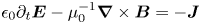 where
where

In order to derive these relations, one makes repeated use of integration by parts in combination with (3.22), (3.23) and
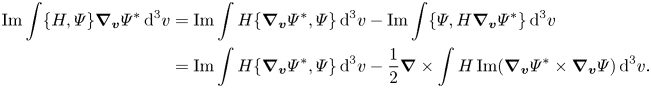
Here, the last equality follows from $\operatorname {Im} \int \{ \varPsi ,H\boldsymbol {\nabla }_{{\boldsymbol {v}}}\varPsi ^*\}\,\textrm {d}^3v=-\operatorname {div}\int H\operatorname {Im}(\boldsymbol {\nabla }_{{\boldsymbol {v}}}\varPsi \otimes \boldsymbol {\nabla }_{{\boldsymbol {v}}}\varPsi ^*)\,\textrm {d}^3v$ by using $\operatorname {Im}\int \varPsi ^*\boldsymbol {\nabla }_{{\boldsymbol {v}}}\boldsymbol {\nabla }_{{\boldsymbol {v}}}\varPsi \,\textrm {d}^3v=0$
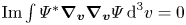 and standard vector algebra. Notice that we have the relation

which follows directly from the KvH equation $\textrm {i}\hbar (\partial _t\varPsi +qm^{-1} {\boldsymbol {E}}\cdot \boldsymbol {\nabla }_{{\boldsymbol {v}}})\varPsi =\hat {{\mathcal {L}}}_{H}\varPsi$ for an arbitrary function $H$
 .
.
3.5. Gauge invariance and charge conservation
So far, nothing has been said about the role of gauge transformations. In this section, we will show how Gauss’ law

arises as usual from gauge invariance. It is well known that Gauss’ law arises from the symmetry of the simultaneous action of gauge transformations over both vector potentials and phase-space quantities. In order to avoid unnecessary difficulties, as explained in Marsden & Weinstein (Reference Marsden and Weinstein1981/82), it is convenient to study the properties of gauge transformations in terms of the canonical coordinates $({\boldsymbol {x}},{\boldsymbol {p}})$ . In particular, besides the standard gauge transformation on the electromagnetic quantities $({\boldsymbol {A}},{\boldsymbol {E}})\mapsto ({\boldsymbol {A}}+\boldsymbol {\nabla }\chi ,{\boldsymbol {E}})$
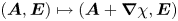 , phase-space coordinates undergo momentum translations of the type $({\boldsymbol {x}},{\boldsymbol {p}})\mapsto ({\boldsymbol {x}},{\boldsymbol {p}}+q\boldsymbol {\nabla }\chi )$
 . In turn, this produces an action of gauge transformations on the phase-space density that is $f({\boldsymbol {x}},{\boldsymbol {p}})=f({\boldsymbol {x}},{\boldsymbol {p}}-q\boldsymbol {\nabla }\chi )$
 . The latter is a type of canonical transformation, which will be the starting point of our discussion.
In order to examine the role of gauge transformations, we have to construct an action of momentum translations on the space of KvH wavefunctions. If we were dealing with KvN theory, this would be simply given by $\varPsi _\text { KvN}({\boldsymbol {x}},{\boldsymbol {p}})\mapsto \varPsi _\text { KvN}({\boldsymbol {x}},{\boldsymbol {p}}-q\boldsymbol {\nabla }\chi )$ . However, KvH wavefunctions also carry a phase factor which we now turn to. If $\boldsymbol {\eta }({\boldsymbol {x}},{\boldsymbol {p}})=({\boldsymbol {x}},{\boldsymbol {p}}+q\boldsymbol {\nabla }\chi )$
 identifies a momentum translation, (3.5) yields

so that (up to irrelevant constants) $\varphi =-q\chi$ and in this case the phase-space function $\varphi$
 depends only on the spatial coordinates ${\boldsymbol {x}}$
 . Then, since $\chi (\boldsymbol {\eta }^{-1}({\boldsymbol {z}}))=\chi ({\boldsymbol {x}})$
 , we are led to the following unitary action $\varPsi _\text { KvH}\mapsto U_{\eta }\varPsi _\text { KvH}$
 of momentum translations on KvH wavefunctions:

Upon dropping the subscript ‘KvH’, we will now show that the Hamiltonian (3.17a,b) is invariant under the gauge transformation

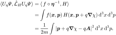
Evidently, $h_\text { Max}$ in (2.26) is manifestly gauge invariant and thus here we consider the first term $\langle \varPsi ,\hat {{\mathcal {L}}}_H \varPsi \rangle$
 . The gauge invariance of this functional is an immediate consequence of the fact that the phase-space density (3.10) identifies an equivariant momentum map. Indeed, since momentum translations are canonical transformations, we can use (3.11) to write
Then, the transformation ${\boldsymbol {A}}\mapsto {\boldsymbol {A}}+\boldsymbol {\nabla }\chi$ leads to overall gauge invariance of $\langle \varPsi ,\hat {{\mathcal {L}}}_H \varPsi \rangle$
 .
.
At this point, we have characterized the gauge transformations that leave the Hamiltonian $h(\varPsi ,{\boldsymbol {A}},{\boldsymbol {E}})=\langle \varPsi ,\hat {{\mathcal {L}}}_H \varPsi \rangle +h_\text {Max}({\boldsymbol {E}},{\boldsymbol {A}})$ invariant and we are ready to present the associated conserved quantity. Here, we shall proceed once again by exploiting momentum maps: since the action of gauge transformations on $(\varPsi ,{\boldsymbol {A}},{\boldsymbol {E}})$
 leaves the Hamiltonian invariant, the momentum map associated with this action is conserved by the dynamics. This momentum map must satisfy the defining relation (2.21). In this case, the Poisson bracket is given by (3.18) and we have $M=L^2(T^*Q)\times T^*\varOmega ^1(Q)$
 , where $\varOmega ^1(Q)$
 denotes the space of differential one-forms on $Q=\Bbb {R}^3$
 . As discussed in Marsden & Weinstein (Reference Marsden and Weinstein1981/82), the Lie algebra of gauge transformations is identified with smooth scalar functions $\xi ({\boldsymbol {x}})$
 on $Q$
 , so that their infinitesimal generator reads

Then, upon writing the momentum map

and computing $\langle {\mathcal {J}}(\varPsi ,{\boldsymbol {A}},{\boldsymbol {E}}),\xi \rangle =-\epsilon _0\langle {\boldsymbol {E}},\boldsymbol {\nabla }\xi \rangle -q\langle \varPsi ,\hat {{\mathcal {L}}}_{\xi }\varPsi \rangle$ , one indeed verifies (2.21). Thus, Gauss’ law (3.29) emerges as the zero-level set of a conserved momentum map associated with the action of gauge transformations.
We conclude our discussion by noticing that, while the Hamiltonian (3.17a,b) is gauge invariant, its dependence on ${\boldsymbol {A}}$ cannot be generally expressed only in terms of the magnetic field ${\boldsymbol {B}}=\boldsymbol {\nabla }\times {\boldsymbol {A}}$
 . While this is precisely what happens also in the standard canonical treatment of the Maxwell–Vlasov system, here, we observe that this feature persists after changing to non-canonical coordinates and this is due to the presence of the Lagrangian function in the prequantum operator (3.22). As proposed in Marsden & Weinstein (Reference Marsden and Weinstein1981/82), one can still write the Hamiltonian $h(\varPsi ,{\boldsymbol {A}},{\boldsymbol {E}})$
 in (3.25) in terms of $(\varPsi ,{\boldsymbol {B}},{\boldsymbol {E}})$
 at the expenses of fixing a convenient gauge such as the Coulomb gauge or the Poincaré gauge. For example, the Coulomb gauge yields ${\boldsymbol {A}}=\boldsymbol {\nabla }\times (\varDelta ^{-1}{\boldsymbol {B}})$
 , which can then be replaced in the expression (3.22) of the prequantum operator. Then, the Poisson bracket (3.21) also changes according to the familiar chain rule relation $\delta /\delta {\boldsymbol {A}}=\boldsymbol {\nabla }\times \delta /\delta {\boldsymbol {B}}$
 .
.
4. Discussion
The KvN and KvH equations represent two valid approaches to developing a Hilbert-space formulation of classical mechanics on phase space. Both approaches lead to a generalized Clebsch representation for the PDF $f$ . A specific choice of the complex phase factor allows this Clebsch representation for f to become equal to the Koopman prescription $\left |\varPsi \right |^2$
 . However, this choice requires the phase factor to become singular.
In both formulations, the complex phase factor is generally involved in reproducing the classical dynamics. In fact, for the KvN formulation, the additional phase degree of freedom is formally required for obtaining a canonical variational formulation. This canonical KvN-Maxwell formulation parallels the development of the canonical KvH–Maxwell formulation, and can be obtained from the results of § 3 by simply eliminating the Lagrangian from the definition of $\hat {{\mathcal {L}}}_{H}$ . In fact, this canonical KvN–Maxwell formulation has been treated in Neiss (Reference Neiss2019) in the electrostatic limit. Alternatively, in order to eliminate the need to include the phase in the KvN dynamics, a non-canonical Poisson bracket was determined that reduces to the standard Vlasov bracket for functionals that depend only on $|\varPsi |^2$
 . In this case, the phase becomes completely irrelevant and can be set to be identically zero.
The ‘pre-quantum’ KvH formulation begins to bridge the gap between the classical and quantum mechanical dynamics by providing a physically motivated prescription for the evolution of the phase factor that agrees with the semiclassical $\hbar \rightarrow 0$ limit. Thus, the prequantum KvH equation can begin to describe some of the important physical consequences of coupling a classical system to a truly quantum system (Bondar et al. Reference Bondar, Gay-Balmaz and Tronci2019; Gay-Balmaz & Tronci Reference Gay-Balmaz and Tronci2019; Tronci & Gay-Balmaz Reference Tronci and Gay-Balmaz2021). In contrast, the KvN formulation, with a trivial phase dynamics, is perhaps better considered to correspond to the diagonal part of the density matrix.
In dealing with both canonical and non-canonical structures, some comments on their numerical aspects are also in place. Indeed, both symplectic numerical integrators and quantum simulation algorithms are well understood for canonical Hamiltonian systems, but not for non-canonical systems with an arbitrary Poisson bracket. While this makes the canonical KvN and KvH formulations more amenable to the development of numerical integration techniques that preserve conservation laws, it also motivates future research on developing numerical methods that target the new non-canonical KvN formulation derived here.
Both approaches can be used to develop a ‘quantum’ representation of the classical Liouville equation and both can be simulated on a quantum computer. However, once the Koopman equation is coupled to Maxwell's equations, one obtains a coupled system of nonlinear partial differential equations. It is only possible to efficiently simulate these equations using a quantum computer if they are embedded within a unitary linear system of equations. This can be done by simulating the classical statistical probability density, ${\mathscr F}(\varPsi ,{\boldsymbol {A}},{\boldsymbol {E}};t,{\boldsymbol {x}})$ , for the fields at every point in space–time. As described in Joseph (Reference Joseph2020), the Liouville equation for ${\mathscr F}$
 can be simulated efficiently on a quantum computer. Understanding the complexity of quantum simulation for each of these Koopman–Maxwell formulations is an important topic for future research.
Acknowledgments
We wish to thank our colleagues Denys Bondar, Joshua Burby, François Gay-Balmaz, John Finn, Michael Kraus, Omar Maj, and Philip Morrison for several interesting discussions on this and related topics.
Editor Hong Qin thanks the referees for their advice in evaluating this article.
Funding
The work of C.T. is partially supported by the Royal Society, UK. The work of I.J. was performed under the auspices of the U.S. Department of Energy (DOE) by Lawrence Livermore National Laboratory (LLNL) under Contract DE-AC52- 07NA27344. I.J. was supported by the DOE Office of Fusion Energy Sciences ‘Quantum Leap for Fusion Energy Sciences’ project FWP-SCW1680 and by LLNL Laboratory Directed Research and Development Project 19-FS-072.
Declaration of interests
The authors report no conflict of interest.
Author contributions
Both authors contributed equally to the development of this work.

 Open access