1 Introduction
Magnetic reconnection is a process whereby magnetic energy is converted locally into particle heat and kinetic energy via some mechanism of effective magnetic dissipation that allows for a change of magnetic field line connectivity. Magnetic reconnection is ubiquitous in space and laboratory plasmas, and is believed to be at the heart of many observed phenomena, such as solar flares (Masuda et al. Reference Masuda, Kosugi, Hara, Tsuneta and Ogawara1994; Su et al. Reference Su, Veronig, Holman, Dennis, Wang, Temmer and Gan2013), geomagnetic substorms (Angelopoulos et al. Reference Angelopoulos, Runov, Zhou, Turner, Kiehas, Li and Shinohara2013) and sawtooth crashes in tokamaks (Kadomtsev Reference Kadomtsev1975; Yamada et al. Reference Yamada, Levinton, Pompherey, Budny, Manickam and Nagayama1994). Apart from these transient events, reconnection is also invoked in coronal heating models in different extensions of the nanoflare scenario (Parker Reference Parker1988; Rappazzo et al. Reference Rappazzo, Velli, Einaudi and Dahlburg2008), and plays a fundamental role during dynamo processes in primordial galaxy clusters (Schekochihin et al. Reference Schekochihin, Cowley, Kulsrud, Hammett and Sharma2005).
Several phenomena in which magnetic reconnection is thought to take place exhibit an explosive character, in the sense that magnetic energy can be stored over a long period of time and then suddenly released on a time scale comparable with the macroscopic ideal Alfvén time
 $\unicode[STIX]{x1D70F}_{A}=L/v_{A}$
, where
$\unicode[STIX]{x1D70F}_{A}=L/v_{A}$
, where
 $L$
is the macroscopic length of the system and
$L$
is the macroscopic length of the system and
 $v_{A}=B_{0}/\sqrt{4\unicode[STIX]{x03C0}\unicode[STIX]{x1D70C}_{0}}$
the Alfvén speed defined through typical values of magnetic field magnitude
$v_{A}=B_{0}/\sqrt{4\unicode[STIX]{x03C0}\unicode[STIX]{x1D70C}_{0}}$
the Alfvén speed defined through typical values of magnetic field magnitude
 $B_{0}$
and plasma mass density
$B_{0}$
and plasma mass density
 $\unicode[STIX]{x1D70C}_{0}$
. For many years, studies of reconnection stumbled on understanding how fast reconnection is triggered. The major difficulty came from the fact that the traditional models of reconnection stemming from the original Sweet–Parker mechanism (Parker Reference Parker1957; Sweet Reference Sweet1958) or from the instability of macroscopic current sheets (Furth, Killeen & Rosenbluth Reference Furth, Killeen and Rosenbluth1963), dating back to the 1960s, were clearly inadequate to explain the observed sudden release of magnetic energy, as such models predict magnetic reconnection time scales – scaling with a positive power of
$\unicode[STIX]{x1D70C}_{0}$
. For many years, studies of reconnection stumbled on understanding how fast reconnection is triggered. The major difficulty came from the fact that the traditional models of reconnection stemming from the original Sweet–Parker mechanism (Parker Reference Parker1957; Sweet Reference Sweet1958) or from the instability of macroscopic current sheets (Furth, Killeen & Rosenbluth Reference Furth, Killeen and Rosenbluth1963), dating back to the 1960s, were clearly inadequate to explain the observed sudden release of magnetic energy, as such models predict magnetic reconnection time scales – scaling with a positive power of
 $S$
, where
$S$
, where
 $S=Lv_{A}/\unicode[STIX]{x1D702}\simeq 10^{6}-10^{14}$
is the macroscopic Lundquist number,
$S=Lv_{A}/\unicode[STIX]{x1D702}\simeq 10^{6}-10^{14}$
is the macroscopic Lundquist number,
 $\unicode[STIX]{x1D702}$
being the magnetic diffusivity – that are far too long to be of any consequence. Several attempts involved locally enhancing the value of diffusivity by invoking anomalous resistivities to make the Sweet–Parker current layer transition to the fast, steady-state Petschek configuration (Petschek Reference Petschek and Hess1964). However, as discussed, e.g. in Shibata & Tanuma (Reference Shibata and Tanuma2001), these also require the formation of extremely small scales in the plasma.
$\unicode[STIX]{x1D702}$
being the magnetic diffusivity – that are far too long to be of any consequence. Several attempts involved locally enhancing the value of diffusivity by invoking anomalous resistivities to make the Sweet–Parker current layer transition to the fast, steady-state Petschek configuration (Petschek Reference Petschek and Hess1964). However, as discussed, e.g. in Shibata & Tanuma (Reference Shibata and Tanuma2001), these also require the formation of extremely small scales in the plasma.
The aim of the present review is to discuss how the difficulty of apparently slow reconnection has been overcome, following the works of Biskamp (Reference Biskamp1986), studies of the plasmoid instability (Loureiro, Schekochihin & Uzdensky Reference Loureiro, Schekochihin and Uzdensky2007) and the fractal reconnection scenario introduced by Shibata & Tanuma (Reference Shibata and Tanuma2001), with emphasis on research carried out by the present authors and in particular on the ‘ideal’ tearing scenario introduced in Pucci & Velli (Reference Pucci and Velli2014). Magnetic reconnection has been the subject of intense research both theoretically and observationally, and in very different physical as well as astrophysical contexts. A complete review on the subject would go well beyond the purpose of the present paper. Here we have tried to include most of the recent papers pertaining to fast reconnection, although the discussion may be brief. A longer review can however be found for instance in Yamada, Kulsrud & Ji (Reference Yamada, Kulsrud and Ji2010).
Over the past decades a vast body of literature has focussed on what might accelerate reconnection speed up to realistic values. For the most part, these works approach the problem by studying (two-dimensional) magnetic reconnection at a single X-point, usually imposed by deforming an initially thick current sheet. The ensuing dynamics at the X-point (sometimes called the developmental phase) eventually leads to an inner current sheet (or diffusion region), in which reconnection is studied by assuming a steady state (or asymptotic phase) is reached. Two major scenarios for onset of fast reconnection have emerged in this way (see also Daughton & Roytershteyn Reference Daughton and Roytershteyn2012; Cassak & Drake Reference Cassak and Drake2013; Huang & Bhattacharjee Reference Huang and Bhattacharjee2013; Loureiro & Uzdensky Reference Loureiro and Uzdensky2015).

Figure 1. Sweet–Parker model. The diffusion region, in yellow, has an inverse aspect ratio
 $a_{SP}/L$
. Coloured arrows represent the plasma flow into and outward the diffusion region.
$a_{SP}/L$
. Coloured arrows represent the plasma flow into and outward the diffusion region.
In resistive magnetohydrodynamics (MHD), numerical simulations show that slowly reconnecting current sheets reminiscent of the Sweet–Parker model (SP) arise from the X-point. The basic SP configuration is shown in figure 1: the current sheet has an inverse aspect ratio
 $a_{SP}/L\sim S^{-1/2}$
, maintained by a continuous inflow of plasma at speed
$a_{SP}/L\sim S^{-1/2}$
, maintained by a continuous inflow of plasma at speed
 $u_{in}\ll v_{A}$
which convects the upstream magnetic field
$u_{in}\ll v_{A}$
which convects the upstream magnetic field
 $\boldsymbol{B}_{0}$
into the diffusion region, and by an outflow at speed
$\boldsymbol{B}_{0}$
into the diffusion region, and by an outflow at speed
 $u_{out}\simeq v_{A}$
which drags the reconnected magnetic field lines outwards, along the sheet; the resulting Alfvén-normalized reconnection rate is
$u_{out}\simeq v_{A}$
which drags the reconnected magnetic field lines outwards, along the sheet; the resulting Alfvén-normalized reconnection rate is
 $u_{in}/u_{out}\sim a_{SP}/L\sim S^{-1/2}$
, assuming the steady-state configuration remains stable. Once computational power allowed to study systems at larger values of
$u_{in}/u_{out}\sim a_{SP}/L\sim S^{-1/2}$
, assuming the steady-state configuration remains stable. Once computational power allowed to study systems at larger values of
 $S$
(
$S$
(
 $S\gtrsim 10^{4}$
), it became clear that SP-like sheets become unstable to tearing (Biskamp Reference Biskamp1986, Reference Biskamp2000), the latter inducing the growth of a large number of magnetic islands (plasmoids). In this regard, linear stability analysis shows that SP sheets are highly unstable to a super-Alfvénic tearing instability – with a growth rate scaling with a positive power of
$S\gtrsim 10^{4}$
), it became clear that SP-like sheets become unstable to tearing (Biskamp Reference Biskamp1986, Reference Biskamp2000), the latter inducing the growth of a large number of magnetic islands (plasmoids). In this regard, linear stability analysis shows that SP sheets are highly unstable to a super-Alfvénic tearing instability – with a growth rate scaling with a positive power of
 $S$
,
$S$
,
 $\unicode[STIX]{x1D6FE}_{SP}\unicode[STIX]{x1D70F}_{A}\sim S^{1/4}$
– as convincingly proved by Loureiro et al. (Reference Loureiro, Schekochihin and Uzdensky2007), Loureiro, Schekochihin & Uzdensky (Reference Loureiro, Schekochihin and Uzdensky2013). Though such an instability demonstrates the possibility of fast reconnection already in resistive MHD, Pucci & Velli (Reference Pucci and Velli2014) pointed out that the growth rate, which diverges in the ideal limit
$\unicode[STIX]{x1D6FE}_{SP}\unicode[STIX]{x1D70F}_{A}\sim S^{1/4}$
– as convincingly proved by Loureiro et al. (Reference Loureiro, Schekochihin and Uzdensky2007), Loureiro, Schekochihin & Uzdensky (Reference Loureiro, Schekochihin and Uzdensky2013). Though such an instability demonstrates the possibility of fast reconnection already in resistive MHD, Pucci & Velli (Reference Pucci and Velli2014) pointed out that the growth rate, which diverges in the ideal limit
 $S\rightarrow \infty$
, poses consistency problems, since magnetic reconnection is prohibited in ideal MHD. In other words, they questioned the realizability of current sheets with excessively large aspect ratios, such as SP, which, when taking the ideal limit starting from resistive MHD, reach an infinite growth rate, i.e. become unstable on time scales which at large enough
$S\rightarrow \infty$
, poses consistency problems, since magnetic reconnection is prohibited in ideal MHD. In other words, they questioned the realizability of current sheets with excessively large aspect ratios, such as SP, which, when taking the ideal limit starting from resistive MHD, reach an infinite growth rate, i.e. become unstable on time scales which at large enough
 $S$
are much shorter than any conceivable dynamical time required to set-up the corresponding configuration. Although this issue of reconnection speed was implicitly recognized in Loureiro et al. (Reference Loureiro, Schekochihin and Uzdensky2007) and many other works, (Bhattacharjee et al.
Reference Battacharjee, Huang, Yang and Rogers2009; Cassak & Drake Reference Cassak and Drake2009; Samtaney et al.
Reference Samtaney, Loureiro, Uzdensky and Schekochihin2009; Huang & Bhattacharjee Reference Huang and Bhattacharjee2010; Uzdensky, Loureiro & Schekochihin Reference Uzdensky, Loureiro and Schekochihin2010; Loureiro et al.
Reference Loureiro, Samtaney, Schekochihin and Uzdensky2012; Ni et al.
Reference Ni, Kliem, Lin and Wu2015) the discussion of the onset of fast tearing has mostly remained anchored to the Sweet–Parker sheet framework.
$S$
are much shorter than any conceivable dynamical time required to set-up the corresponding configuration. Although this issue of reconnection speed was implicitly recognized in Loureiro et al. (Reference Loureiro, Schekochihin and Uzdensky2007) and many other works, (Bhattacharjee et al.
Reference Battacharjee, Huang, Yang and Rogers2009; Cassak & Drake Reference Cassak and Drake2009; Samtaney et al.
Reference Samtaney, Loureiro, Uzdensky and Schekochihin2009; Huang & Bhattacharjee Reference Huang and Bhattacharjee2010; Uzdensky, Loureiro & Schekochihin Reference Uzdensky, Loureiro and Schekochihin2010; Loureiro et al.
Reference Loureiro, Samtaney, Schekochihin and Uzdensky2012; Ni et al.
Reference Ni, Kliem, Lin and Wu2015) the discussion of the onset of fast tearing has mostly remained anchored to the Sweet–Parker sheet framework.
Alternatively, it has been suggested that if ion scales are of the order of, or larger than, the thickness of the SP sheet, then two-fluid effects enhance the reconnection rate via what is usually called Hall-mediated reconnection. It was already known that the Hall term in Ohm’s law increases the reconnection speed because of the excitation of dispersive waves, e.g. whistler waves (Terasawa Reference Terasawa1983; Mandt, Denton & Drake Reference Mandt, Denton and Drake1994; Biskamp, Schwartz & Drake Reference Biskamp, Schwartz and Drake1995; Rogers et al.
Reference Rogers, Denton, Drake and Shay2001). To be more specific, it was argued, on the basis of numerical simulations, that large reconnection rates should be achieved during the nonlinear asymptotic phase, regardless of the mechanisms allowing reconnection (e.g. resistivity or electron inertia in collisionless reconnection), essentially because the Hall term modifies the structure of the diffusion region that becomes localized at scales of the order of the ion inertial length (Shay et al.
Reference Shay, Drake, Rogers and Denton1999, Reference Shay, Drake, Swisdak and Rogers2004; Cassak, Shay & Drake Reference Cassak, Shay and Drake2005; Drake, Shay & Swisdak Reference Drake, Shay and Swisdak2008; Shepherd & Cassak Reference Shepherd and Cassak2010). However, there is still no general agreement on whether and how the reconnection rate depends on the system size
 $L$
and plasma parameters such as the ion and electron inertial length
$L$
and plasma parameters such as the ion and electron inertial length
 $d_{i}$
and
$d_{i}$
and
 $d_{e}$
or resistivity, in the presence of the Hall term (Porcelli et al.
Reference Porcelli, Borgogno, Califano, Grasso, Ottaviani and Pegoraro2002; Battacharjee, Germaschewski & Ng Reference Battacharjee, Germaschewski and Ng2005). More recent numerical results from PIC (particle in cell) simulations have also cast doubt on the necessity of exciting dispersive waves to reach higher reconnection rates (Liu et al.
Reference Liu, Daughton, Karimabadi, Li and Peter2014). The robustness of the steady-state configuration reached during the asymptotic phase, and seen in several numerical studies (Birn et al.
Reference Birn, Drake, Shay, Rogers and Denton2001; Shepherd & Cassak Reference Shepherd and Cassak2010), has been called into question by both PIC and Hall-MHD simulations employing open boundaries or larger system sizes (Daughton, Scudder & Karimabadi Reference Daughton, Scudder and Karimabadi2006; Klimas, Hesse & Zenitani Reference Klimas, Hesse and Zenitani2008; Huang, Bhattacharjee & Sullivan Reference Huang, Bhattacharjee and Sullivan2011). These works provide some evidence that a final steady-state configuration may not always exist in Hall reconnection, and that the thin sheet constituting the diffusion region tends to stretch along the outflow direction until it becomes unstable to generation of secondary plasmoids. This would point to a strong analogy with the dynamics of thin current sheets found in resistive MHD.
$d_{e}$
or resistivity, in the presence of the Hall term (Porcelli et al.
Reference Porcelli, Borgogno, Califano, Grasso, Ottaviani and Pegoraro2002; Battacharjee, Germaschewski & Ng Reference Battacharjee, Germaschewski and Ng2005). More recent numerical results from PIC (particle in cell) simulations have also cast doubt on the necessity of exciting dispersive waves to reach higher reconnection rates (Liu et al.
Reference Liu, Daughton, Karimabadi, Li and Peter2014). The robustness of the steady-state configuration reached during the asymptotic phase, and seen in several numerical studies (Birn et al.
Reference Birn, Drake, Shay, Rogers and Denton2001; Shepherd & Cassak Reference Shepherd and Cassak2010), has been called into question by both PIC and Hall-MHD simulations employing open boundaries or larger system sizes (Daughton, Scudder & Karimabadi Reference Daughton, Scudder and Karimabadi2006; Klimas, Hesse & Zenitani Reference Klimas, Hesse and Zenitani2008; Huang, Bhattacharjee & Sullivan Reference Huang, Bhattacharjee and Sullivan2011). These works provide some evidence that a final steady-state configuration may not always exist in Hall reconnection, and that the thin sheet constituting the diffusion region tends to stretch along the outflow direction until it becomes unstable to generation of secondary plasmoids. This would point to a strong analogy with the dynamics of thin current sheets found in resistive MHD.
Linear analysis of the tearing mode in resistive MHD proves that there exists a critical current sheet with an inverse aspect ratio
 $a_{i}/L\sim S^{-1/3}$
(Pucci & Velli Reference Pucci and Velli2014), hence much larger than the SP one, that separates slowly reconnecting sheets (growth rate scaling with a negative power of
$a_{i}/L\sim S^{-1/3}$
(Pucci & Velli Reference Pucci and Velli2014), hence much larger than the SP one, that separates slowly reconnecting sheets (growth rate scaling with a negative power of
 $S$
), from those exhibiting super-Alfvénic plasmoid instabilities (growth rate diverging with
$S$
), from those exhibiting super-Alfvénic plasmoid instabilities (growth rate diverging with
 $S$
), and that this has the proper convergence properties to ideal MHD: critical current sheets are unstable to a tearing mode growing at a rate independent from
$S$
), and that this has the proper convergence properties to ideal MHD: critical current sheets are unstable to a tearing mode growing at a rate independent from
 $S$
and, in this sense, the instability is ‘ideal’. The existence of ‘ideal’ tearing therefore implies the impossibility of constructing any configuration corresponding to sheets thinner than critical, such as the paradigmatic Sweet–Parker sheet, suggesting a different route to the triggering of fast reconnection. At the same time, as we shall see, reasoning in terms of the rescaling arguments provides a clear predictive pathway to the critical events involved in a dynamics that will trigger fast reconnection, providing an alternative framework within which the many and different results previously obtained in simulations may be reinterpreted. It is worth mentioning that one of the major difficulties in this kind of numerical simulation concerns achieving sufficiently large Lundquist numbers. At the intermediate Lundquist numbers usual to MHD simulations, say
$S$
and, in this sense, the instability is ‘ideal’. The existence of ‘ideal’ tearing therefore implies the impossibility of constructing any configuration corresponding to sheets thinner than critical, such as the paradigmatic Sweet–Parker sheet, suggesting a different route to the triggering of fast reconnection. At the same time, as we shall see, reasoning in terms of the rescaling arguments provides a clear predictive pathway to the critical events involved in a dynamics that will trigger fast reconnection, providing an alternative framework within which the many and different results previously obtained in simulations may be reinterpreted. It is worth mentioning that one of the major difficulties in this kind of numerical simulation concerns achieving sufficiently large Lundquist numbers. At the intermediate Lundquist numbers usual to MHD simulations, say
 $S\simeq 10^{4}-10^{6}$
, the SP sheet is at most 10 times thinner than the critical current sheet predicted by the ‘ideal’ tearing theory. Moreover, the possible presence of plasma flows along the current sheet tends to stabilize the tearing mode (Bulanov, Syrovatskiǐ & Sakai Reference Bulanov, Syrovatskiǐ and Sakai1978), inducing the formation of more elongated current sheets, that is, of layers having inverse aspect ratios smaller than
$S\simeq 10^{4}-10^{6}$
, the SP sheet is at most 10 times thinner than the critical current sheet predicted by the ‘ideal’ tearing theory. Moreover, the possible presence of plasma flows along the current sheet tends to stabilize the tearing mode (Bulanov, Syrovatskiǐ & Sakai Reference Bulanov, Syrovatskiǐ and Sakai1978), inducing the formation of more elongated current sheets, that is, of layers having inverse aspect ratios smaller than
 $S^{-1/3}$
(in the resistive case). Therefore, with the Lundquist number not sufficiently large, the distinction between ‘ideal’ tearing framework and SP-plasmoids might be hard to observe, although the departure from the SP-plasmoid framework should become increasingly obvious with increasing
$S^{-1/3}$
(in the resistive case). Therefore, with the Lundquist number not sufficiently large, the distinction between ‘ideal’ tearing framework and SP-plasmoids might be hard to observe, although the departure from the SP-plasmoid framework should become increasingly obvious with increasing
 $S$
.
$S$
.
Throughout this review we summarize and complement recent results stemming from the ‘ideal’ tearing idea, obtained from both linear theory and nonlinear numerical simulations, providing a coherent perspective on recent studies and their relation to previous models: ‘ideal’ tearing can explain the trigger of fast reconnection occurring on critically unstable current sheets and can provide a guide – at least in two dimensions – to the nonlinear evolution with a model that describes the different stages of its evolution. Although we focus mainly on the resistive MHD description of the plasma, the ‘ideal’ tearing idea can be extended to other regimes, such as two fluid, Hall-MHD and so on to completely kinetic ones, providing a unified and self-consistent framework for the onset of fast reconnection. In this paper we briefly discuss the application to simple kinetic models of collisionless reconnection.
The paper is organized as follows: in § 2 we summarize the theory of the tearing mode instability in its traditional form, in order to prepare the ground for the ‘ideal’ tearing, that we discuss in § 3; in § 4 we approach the problem of the trigger of fast reconnection and we propose a new scenario relying on the ‘ideal’ tearing; in § 5 we show that the trigger of fast reconnection via ‘ideal’ tearing can describe the evolution of a disrupting current sheet during its different nonlinear stages, characterized by a recursive sequence of tearing instabilities, and we compare our results with previous existent models in § 6; a final summary and discussion are deferred to § 7. For the sake of clarity, we mention here that in §§ 2 and 3 we show results that have been obtained from linear theory by solving numerically the system of ordinary differential equations of the eigenvalue problem of the tearing mode, with an adaptive finite difference scheme based on Newton iteration (Lentini & Pereira Reference Lentini and Pereyra1987); in §§ 4 and 5 we show results obtained from 2 and
 $1/2$
dimensional, fully nonlinear resistive MHD simulations.
$1/2$
dimensional, fully nonlinear resistive MHD simulations.

Figure 2. Tearing mode instability. Coloured arrows represent the perturbed plasma flows into and outward the X-point.
2 Background: the tearing mode instability
Magnetic reconnection can arise spontaneously within current sheets as the outcome of an internal tearing instability when the non-ideal terms in Ohm’s law, resistivity in our case, are taken into account. Tearing modes have been extensively studied in the simpler case of an infinite (one-dimensional) sheet both in the linear (Furth et al. Reference Furth, Killeen and Rosenbluth1963) and nonlinear (Rutherford Reference Rutherford1973; Waelbroeck Reference Waelbroeck1989) regime. Below, we briefly summarize the basic properties of the instability, obtained from linear analysis in the resistive MHD framework. We assume, as usually done, an incompressible, homogeneous density plasma.
Tearing modes are long-wavelength modes, that is, unstable perturbations have wavelengths larger than the shear length (or thickness)
 $a$
of the equilibrium magnetic field
$a$
of the equilibrium magnetic field
 $\boldsymbol{B}$
. Such unstable modes lead to the growth of magnetic islands via reconnection at the magnetic neutral line, or, more generally, on ‘resonant’ surfaces where
$\boldsymbol{B}$
. Such unstable modes lead to the growth of magnetic islands via reconnection at the magnetic neutral line, or, more generally, on ‘resonant’ surfaces where
 $\boldsymbol{k}\boldsymbol{\cdot }\boldsymbol{B}=0$
,
$\boldsymbol{k}\boldsymbol{\cdot }\boldsymbol{B}=0$
,
 $\boldsymbol{k}$
being the wave vector of the perturbation along the sheet (figure 2). Instability grows on a time scale
$\boldsymbol{k}$
being the wave vector of the perturbation along the sheet (figure 2). Instability grows on a time scale
 ${\sim}1/\unicode[STIX]{x1D6FE}$
that is intermediate between the dissipative time of the equilibrium magnetic field,
${\sim}1/\unicode[STIX]{x1D6FE}$
that is intermediate between the dissipative time of the equilibrium magnetic field,
 $\unicode[STIX]{x1D70F}_{\unicode[STIX]{x1D702}}=a^{2}/\unicode[STIX]{x1D702}$
, and the Alfvén crossing time
$\unicode[STIX]{x1D70F}_{\unicode[STIX]{x1D702}}=a^{2}/\unicode[STIX]{x1D702}$
, and the Alfvén crossing time
 $\bar{\unicode[STIX]{x1D70F}}=a/v_{A}$
based on the thickness
$\bar{\unicode[STIX]{x1D70F}}=a/v_{A}$
based on the thickness
 $a$
. It is worth noting that since MHD does not have any intrinsic scale, lengths are traditionally normalized to the thickness
$a$
. It is worth noting that since MHD does not have any intrinsic scale, lengths are traditionally normalized to the thickness
 $a$
of the sheet – differently from the SP model in which, instead,
$a$
of the sheet – differently from the SP model in which, instead,
 $L$
is the macroscopic length – whereas time is normalized to
$L$
is the macroscopic length – whereas time is normalized to
 $\bar{\unicode[STIX]{x1D70F}}$
. For the sake of clarity, we therefore label with an overbar the quantities defined through the current sheet thickness,
$\bar{\unicode[STIX]{x1D70F}}$
. For the sake of clarity, we therefore label with an overbar the quantities defined through the current sheet thickness,
 $\bar{\unicode[STIX]{x1D70F}}=a/v_{A}$
and
$\bar{\unicode[STIX]{x1D70F}}=a/v_{A}$
and
 $\bar{S}=av_{A}/\unicode[STIX]{x1D702}$
.
$\bar{S}=av_{A}/\unicode[STIX]{x1D702}$
.
Since resistivity is negligible (or rather
 $\bar{S}^{-1}\ll 1$
) everywhere except close to the resonant surface, tearing modes exhibit a quasi-singular behaviour in a small boundary layer of thickness
$\bar{S}^{-1}\ll 1$
) everywhere except close to the resonant surface, tearing modes exhibit a quasi-singular behaviour in a small boundary layer of thickness
 $\unicode[STIX]{x1D6FF}$
, the inner diffusion region, in which the perturbed magnetic and velocity fields exhibit sharp gradients, and where reconnection can take place. Out of the inner region, where resistivity can be neglected, perturbations smoothly decay to zero far from the resonant surface. An example of the eigenfunctions of the magnetic flux and velocity streamfunctions
$\unicode[STIX]{x1D6FF}$
, the inner diffusion region, in which the perturbed magnetic and velocity fields exhibit sharp gradients, and where reconnection can take place. Out of the inner region, where resistivity can be neglected, perturbations smoothly decay to zero far from the resonant surface. An example of the eigenfunctions of the magnetic flux and velocity streamfunctions
 $\unicode[STIX]{x1D713}$
and
$\unicode[STIX]{x1D713}$
and
 $\unicode[STIX]{x1D719}$
at
$\unicode[STIX]{x1D719}$
at
 $\bar{S}=10^{6}$
is shown in figure 3. In this case, the plotted eigenfunctions correspond to a Harris current sheet equilibrium, which is the one considered most in the literature and has a magnetic field profile
$\bar{S}=10^{6}$
is shown in figure 3. In this case, the plotted eigenfunctions correspond to a Harris current sheet equilibrium, which is the one considered most in the literature and has a magnetic field profile
 $\boldsymbol{B}=B_{0}\tanh (x/a)\hat{\boldsymbol{y}}$
. In perfectly antisymmetric equilibria, as the one chosen here, the eigenfunctions have a well-defined parity: the magnetic flux function is symmetric in
$\boldsymbol{B}=B_{0}\tanh (x/a)\hat{\boldsymbol{y}}$
. In perfectly antisymmetric equilibria, as the one chosen here, the eigenfunctions have a well-defined parity: the magnetic flux function is symmetric in
 $x$
, being proportional to the reconnected magnetic field component at the neutral line, whereas the velocity streamfunction, proportional to the perturbed plasma velocity perpendicular to the sheet, is antisymmetric. As can be seen in figure 3(b), the plasma strongly accelerates while flowing into the inner layer, with the streamfunction ideally diverging as
$x$
, being proportional to the reconnected magnetic field component at the neutral line, whereas the velocity streamfunction, proportional to the perturbed plasma velocity perpendicular to the sheet, is antisymmetric. As can be seen in figure 3(b), the plasma strongly accelerates while flowing into the inner layer, with the streamfunction ideally diverging as
 $\unicode[STIX]{x1D719}/(av_{A})\sim a/x$
for
$\unicode[STIX]{x1D719}/(av_{A})\sim a/x$
for
 $|x/a|\rightarrow 0$
. Resistivity becomes non-negligible close to the neutral line, regularizing the singularity: inside the inner layer, the plasma decelerates to the stagnation point, where it deflects outwards along the sheet, while the magnetic field diffuses and reconnects.
$|x/a|\rightarrow 0$
. Resistivity becomes non-negligible close to the neutral line, regularizing the singularity: inside the inner layer, the plasma decelerates to the stagnation point, where it deflects outwards along the sheet, while the magnetic field diffuses and reconnects.

Figure 3. Tearing eigenfunctions for
 $S=10^{6}$
and
$S=10^{6}$
and
 $ka=0.8$
(small
$ka=0.8$
(small
 $\unicode[STIX]{x1D6E5}^{\prime }$
): magnetic field flux function
$\unicode[STIX]{x1D6E5}^{\prime }$
): magnetic field flux function
 $\unicode[STIX]{x1D713}$
(a) and velocity field streamfunction
$\unicode[STIX]{x1D713}$
(a) and velocity field streamfunction
 $\unicode[STIX]{x1D719}$
(b).
$\unicode[STIX]{x1D719}$
(b).
Instability is fed by the equilibrium current gradients which enter through the parameter
 $\unicode[STIX]{x1D6E5}^{\prime }(k)$
, or for brevity
$\unicode[STIX]{x1D6E5}^{\prime }(k)$
, or for brevity
 $\unicode[STIX]{x1D6E5}^{\prime }$
. The latter is defined as the discontinuity of the logarithmic derivative of the outer flux function when approaching the singular layer, and is a measure of the free energy of the system. The
$\unicode[STIX]{x1D6E5}^{\prime }$
. The latter is defined as the discontinuity of the logarithmic derivative of the outer flux function when approaching the singular layer, and is a measure of the free energy of the system. The
 $\unicode[STIX]{x1D6E5}^{\prime }$
parameter defines the instability threshold condition, instability occurring only when
$\unicode[STIX]{x1D6E5}^{\prime }$
parameter defines the instability threshold condition, instability occurring only when
 $\unicode[STIX]{x1D6E5}^{\prime }>0$
(Furth et al.
Reference Furth, Killeen and Rosenbluth1963; Adler, Kulsrud & White Reference Adler, Kulsrud and White1980). For a Harris current sheet
$\unicode[STIX]{x1D6E5}^{\prime }>0$
(Furth et al.
Reference Furth, Killeen and Rosenbluth1963; Adler, Kulsrud & White Reference Adler, Kulsrud and White1980). For a Harris current sheet
 $\unicode[STIX]{x1D6E5}^{\prime }a=2[(ka)^{-1}-ka]$
, so that the unstable modes have wave vector satisfying
$\unicode[STIX]{x1D6E5}^{\prime }a=2[(ka)^{-1}-ka]$
, so that the unstable modes have wave vector satisfying
 $ka<1$
.
$ka<1$
.
The
 $\unicode[STIX]{x1D6E5}^{\prime }$
parameter also controls the linear evolution. There are indeed two regimes that describe the unstable spectrum depending on the value of
$\unicode[STIX]{x1D6E5}^{\prime }$
parameter also controls the linear evolution. There are indeed two regimes that describe the unstable spectrum depending on the value of
 $\unicode[STIX]{x1D6E5}^{\prime }\unicode[STIX]{x1D6FF}$
. One is the so called constant-
$\unicode[STIX]{x1D6E5}^{\prime }\unicode[STIX]{x1D6FF}$
. One is the so called constant-
 $\unicode[STIX]{x1D713}$
regime, traditionally referred to as tearing mode or small
$\unicode[STIX]{x1D713}$
regime, traditionally referred to as tearing mode or small
 $\unicode[STIX]{x1D6E5}^{\prime }$
regime (Furth et al.
Reference Furth, Killeen and Rosenbluth1963). The other one is the non-constant-
$\unicode[STIX]{x1D6E5}^{\prime }$
regime (Furth et al.
Reference Furth, Killeen and Rosenbluth1963). The other one is the non-constant-
 $\unicode[STIX]{x1D713}$
regime, or large
$\unicode[STIX]{x1D713}$
regime, or large
 $\unicode[STIX]{x1D6E5}^{\prime }$
, also known as resistive internal kink (Coppi et al.
Reference Coppi, Galvao, Pellat, Rosenbluth and Rutherford1976). The difference between these two regimes is in the ordering of the derivatives of
$\unicode[STIX]{x1D6E5}^{\prime }$
, also known as resistive internal kink (Coppi et al.
Reference Coppi, Galvao, Pellat, Rosenbluth and Rutherford1976). The difference between these two regimes is in the ordering of the derivatives of
 $\unicode[STIX]{x1D713}$
within the inner layer that leads to two different limiting cases of the dispersion relation (Ara, Basu & Coppi Reference Ara, Basu and Coppi1978): in the small
$\unicode[STIX]{x1D713}$
within the inner layer that leads to two different limiting cases of the dispersion relation (Ara, Basu & Coppi Reference Ara, Basu and Coppi1978): in the small
 $\unicode[STIX]{x1D6E5}^{\prime }$
regime
$\unicode[STIX]{x1D6E5}^{\prime }$
regime
 $\unicode[STIX]{x1D713}^{\prime }\sim \unicode[STIX]{x1D713}\,\unicode[STIX]{x1D6E5}^{\prime }$
and
$\unicode[STIX]{x1D713}^{\prime }\sim \unicode[STIX]{x1D713}\,\unicode[STIX]{x1D6E5}^{\prime }$
and
 $\unicode[STIX]{x1D713}^{\prime \prime }\sim \unicode[STIX]{x1D713}\,\unicode[STIX]{x1D6E5}^{\prime }\unicode[STIX]{x1D6FF}^{-1}$
, that is, in the inner region
$\unicode[STIX]{x1D713}^{\prime \prime }\sim \unicode[STIX]{x1D713}\,\unicode[STIX]{x1D6E5}^{\prime }\unicode[STIX]{x1D6FF}^{-1}$
, that is, in the inner region
 $\unicode[STIX]{x1D713}$
is roughly constant and can be approximated by
$\unicode[STIX]{x1D713}$
is roughly constant and can be approximated by
 $\unicode[STIX]{x1D713}(0)$
, provided
$\unicode[STIX]{x1D713}(0)$
, provided
 $\unicode[STIX]{x1D6E5}^{\prime }\unicode[STIX]{x1D6FF}\ll 1$
; at larger values of
$\unicode[STIX]{x1D6E5}^{\prime }\unicode[STIX]{x1D6FF}\ll 1$
; at larger values of
 $\unicode[STIX]{x1D6E5}^{\prime }$
this approximation breaks down as
$\unicode[STIX]{x1D6E5}^{\prime }$
this approximation breaks down as
 $\unicode[STIX]{x1D713}$
has stronger gradients,
$\unicode[STIX]{x1D713}$
has stronger gradients,
 $\unicode[STIX]{x1D713}^{\prime }\sim \unicode[STIX]{x1D713}\,\unicode[STIX]{x1D6FF}^{-1}$
and
$\unicode[STIX]{x1D713}^{\prime }\sim \unicode[STIX]{x1D713}\,\unicode[STIX]{x1D6FF}^{-1}$
and
 $\unicode[STIX]{x1D713}^{\prime \prime }\sim \unicode[STIX]{x1D713}\,\unicode[STIX]{x1D6FF}^{-2}$
. In particular, the growth rate
$\unicode[STIX]{x1D713}^{\prime \prime }\sim \unicode[STIX]{x1D713}\,\unicode[STIX]{x1D6FF}^{-2}$
. In particular, the growth rate
 $\unicode[STIX]{x1D6FE}$
and the inner layer
$\unicode[STIX]{x1D6FE}$
and the inner layer
 $\unicode[STIX]{x1D6FF}$
scale in these two regimes as
$\unicode[STIX]{x1D6FF}$
scale in these two regimes as
 $$\begin{eqnarray}\displaystyle \unicode[STIX]{x1D6FE}\bar{\unicode[STIX]{x1D70F}}\sim \bar{S}^{-3/5}(ka)^{2/5}(\unicode[STIX]{x1D6E5}^{\prime }a)^{4/5},\quad \frac{\unicode[STIX]{x1D6FF}}{a}\sim \bar{S}^{-2/5}\quad (\unicode[STIX]{x1D6E5}^{\prime }\unicode[STIX]{x1D6FF}\ll 1), & & \displaystyle\end{eqnarray}$$
 $$\begin{eqnarray}\displaystyle \unicode[STIX]{x1D6FE}\bar{\unicode[STIX]{x1D70F}}\sim \bar{S}^{-1/3}(ka)^{2/3},\quad \frac{\unicode[STIX]{x1D6FF}}{a}\sim \bar{S}^{-1/3}\quad (\unicode[STIX]{x1D6E5}^{\prime }\unicode[STIX]{x1D6FF}\gg 1). & & \displaystyle\end{eqnarray}$$
The expressions above can also be found as special cases of a general dispersion relation valid for any given value of the parameter
 $\unicode[STIX]{x1D6E5}^{\prime }$
(Pegoraro & Schep Reference Pegoraro and Schep1986).
$\unicode[STIX]{x1D6E5}^{\prime }$
(Pegoraro & Schep Reference Pegoraro and Schep1986).
Roughly speaking, the small and the large
 $\unicode[STIX]{x1D6E5}^{\prime }$
regimes have wave vectors lying to the right and to the left of the fastest growing mode
$\unicode[STIX]{x1D6E5}^{\prime }$
regimes have wave vectors lying to the right and to the left of the fastest growing mode
 $k_{m}$
, respectively. For example, in the case of a Harris sheet the two regimes correspond to a region in
$k_{m}$
, respectively. For example, in the case of a Harris sheet the two regimes correspond to a region in
 $k$
-space
$k$
-space
 $k_{m}a<ka<1$
in which the growth rate decreases with
$k_{m}a<ka<1$
in which the growth rate decreases with
 $k$
(small
$k$
(small
 $\unicode[STIX]{x1D6E5}^{\prime }$
) and another one
$\unicode[STIX]{x1D6E5}^{\prime }$
) and another one
 $0<ka<k_{m}a$
where the growth rate increases with
$0<ka<k_{m}a$
where the growth rate increases with
 $k$
(large
$k$
(large
 $\unicode[STIX]{x1D6E5}^{\prime }$
). The scaling relations for the fastest growing mode can therefore be obtained by matching the two regimes (Bhattacharjee et al.
Reference Battacharjee, Huang, Yang and Rogers2009; Loureiro et al.
Reference Loureiro, Schekochihin and Uzdensky2013; Del Sarto et al.
Reference Del Sarto, Pucci, Tenerani and Velli2016). Since the expressions for
$\unicode[STIX]{x1D6E5}^{\prime }$
). The scaling relations for the fastest growing mode can therefore be obtained by matching the two regimes (Bhattacharjee et al.
Reference Battacharjee, Huang, Yang and Rogers2009; Loureiro et al.
Reference Loureiro, Schekochihin and Uzdensky2013; Del Sarto et al.
Reference Del Sarto, Pucci, Tenerani and Velli2016). Since the expressions for
 $\unicode[STIX]{x1D6FE}\bar{\unicode[STIX]{x1D70F}}$
given in (2.1)–(2.2) should coincide at the fastest growing mode, the wave vector
$\unicode[STIX]{x1D6FE}\bar{\unicode[STIX]{x1D70F}}$
given in (2.1)–(2.2) should coincide at the fastest growing mode, the wave vector
 $k_{m}$
can be obtained by equating the right-hand side of the growth rate in the small and large
$k_{m}$
can be obtained by equating the right-hand side of the growth rate in the small and large
 $\unicode[STIX]{x1D6E5}^{\prime }$
regimes, respectively. The scaling of the maximum growth rate
$\unicode[STIX]{x1D6E5}^{\prime }$
regimes, respectively. The scaling of the maximum growth rate
 $\unicode[STIX]{x1D6FE}_{m}$
follows directly by either the small or the large
$\unicode[STIX]{x1D6FE}_{m}$
follows directly by either the small or the large
 $\unicode[STIX]{x1D6E5}^{\prime }$
growth rate at
$\unicode[STIX]{x1D6E5}^{\prime }$
growth rate at
 $k=k_{m}$
, leading to
$k=k_{m}$
, leading to
 $$\begin{eqnarray}k_{m}a\sim \bar{S}^{-1/4},\quad \unicode[STIX]{x1D6FE}_{m}\bar{\unicode[STIX]{x1D70F}}\sim \bar{S}^{-1/2},\quad \frac{\unicode[STIX]{x1D6FF}_{m}}{a}\sim \bar{S}^{-1/4}\quad \text{(Fastest growing mode)}.\end{eqnarray}$$
In figure 4 we show the transition from the small to the large
 $\unicode[STIX]{x1D6E5}^{\prime }$
regime by plotting
$\unicode[STIX]{x1D6E5}^{\prime }$
regime by plotting
 $\unicode[STIX]{x1D6FE}\bar{\unicode[STIX]{x1D70F}}$
as a function of
$\unicode[STIX]{x1D6FE}\bar{\unicode[STIX]{x1D70F}}$
as a function of
 $\bar{S}$
at two different wave vectors,
$\bar{S}$
at two different wave vectors,
 $ka=0.01$
(light-blue dots) and
$ka=0.01$
(light-blue dots) and
 $ka=0.05$
(red dots). The dashed lines correspond to the asymptotic scalings of the growth rate given in (2.1)–(2.3). As can be seen, as the Lundquist number
$ka=0.05$
(red dots). The dashed lines correspond to the asymptotic scalings of the growth rate given in (2.1)–(2.3). As can be seen, as the Lundquist number
 $\bar{S}$
increases, the growth rate for a given wave vector moves from large to small
$\bar{S}$
increases, the growth rate for a given wave vector moves from large to small
 $\unicode[STIX]{x1D6E5}^{\prime }$
regimes. The transition is marked by a break in the slope of
$\unicode[STIX]{x1D6E5}^{\prime }$
regimes. The transition is marked by a break in the slope of
 $\unicode[STIX]{x1D6FE}\bar{\unicode[STIX]{x1D70F}}$
when the given wave vector corresponds to the fastest growing mode for a specific pair of
$\unicode[STIX]{x1D6FE}\bar{\unicode[STIX]{x1D70F}}$
when the given wave vector corresponds to the fastest growing mode for a specific pair of
 $\{\unicode[STIX]{x1D6FE}\bar{\unicode[STIX]{x1D70F}},\bar{S}\}_{k=k_{m}}$
, so that the envelope of the break-points for all
$\{\unicode[STIX]{x1D6FE}\bar{\unicode[STIX]{x1D70F}},\bar{S}\}_{k=k_{m}}$
, so that the envelope of the break-points for all
 $k$
values scales as
$k$
values scales as
 $\bar{S}^{-1/2}$
, as expected.
$\bar{S}^{-1/2}$
, as expected.

Figure 4. Growth rate
 $\unicode[STIX]{x1D6FE}\bar{\unicode[STIX]{x1D70F}}$
versus
$\unicode[STIX]{x1D6FE}\bar{\unicode[STIX]{x1D70F}}$
versus
 $\bar{S}$
: transition from the small to the large
$\bar{S}$
: transition from the small to the large
 $\unicode[STIX]{x1D6E5}^{\prime }$
regime for two different wave vectors. Dashed lines represent the asymptotic scalings of the large and small
$\unicode[STIX]{x1D6E5}^{\prime }$
regime for two different wave vectors. Dashed lines represent the asymptotic scalings of the large and small
 $\unicode[STIX]{x1D6E5}^{\prime }$
regimes,
$\unicode[STIX]{x1D6E5}^{\prime }$
regimes,
 $\unicode[STIX]{x1D6FE}\bar{\unicode[STIX]{x1D70F}}\sim \bar{S}^{-1/3}$
and
$\unicode[STIX]{x1D6FE}\bar{\unicode[STIX]{x1D70F}}\sim \bar{S}^{-1/3}$
and
 $\unicode[STIX]{x1D6FE}\bar{\unicode[STIX]{x1D70F}}\sim \bar{S}^{-3/5}$
, respectively, and of the fastest growing mode
$\unicode[STIX]{x1D6FE}\bar{\unicode[STIX]{x1D70F}}\sim \bar{S}^{-3/5}$
, respectively, and of the fastest growing mode
 $\unicode[STIX]{x1D6FE}\bar{\unicode[STIX]{x1D70F}}\sim \bar{S}^{-1/2}$
. The latter envelops the slope breaks occurring at the transition between small and large
$\unicode[STIX]{x1D6FE}\bar{\unicode[STIX]{x1D70F}}\sim \bar{S}^{-1/2}$
. The latter envelops the slope breaks occurring at the transition between small and large
 $\unicode[STIX]{x1D6E5}^{\prime }$
.
$\unicode[STIX]{x1D6E5}^{\prime }$
.
3 Stability of thin current sheets and the ‘ideal’ tearing mode
In the traditional theory of tearing mode the current sheet aspect ratio is fixed and its thickness
 $a$
is assumed to be macroscopic. On the other hand if a current sheet becomes thin enough, both the Alfvén time which normalizes the growth rate and the Lundquist number become smaller and smaller. Therefore, even if the growth rate appears to be small, it might actually be large when physically calculated in terms of macroscopic quantities. Indeed, as first seen by Biskamp (Reference Biskamp1986), the thin SP current sheet appeared to become unstable to fast reconnecting mode once a critical Lundquist number
$a$
is assumed to be macroscopic. On the other hand if a current sheet becomes thin enough, both the Alfvén time which normalizes the growth rate and the Lundquist number become smaller and smaller. Therefore, even if the growth rate appears to be small, it might actually be large when physically calculated in terms of macroscopic quantities. Indeed, as first seen by Biskamp (Reference Biskamp1986), the thin SP current sheet appeared to become unstable to fast reconnecting mode once a critical Lundquist number
 $S_{c}$
of order
$S_{c}$
of order
 $10^{4}$
was passed. It is therefore of interest to consider generic current sheets whose aspect ratio scales with
$10^{4}$
was passed. It is therefore of interest to consider generic current sheets whose aspect ratio scales with
 $S$
as
$S$
as
 $L/a\sim S^{\unicode[STIX]{x1D6FC}}$
, where now the scaling exponent
$L/a\sim S^{\unicode[STIX]{x1D6FC}}$
, where now the scaling exponent
 $\unicode[STIX]{x1D6FC}$
(
$\unicode[STIX]{x1D6FC}$
(
 $\unicode[STIX]{x1D6FC}=1/2$
for SP) is not specified (Bhattacharjee et al.
Reference Battacharjee, Huang, Yang and Rogers2009; Pucci & Velli Reference Pucci and Velli2014). For the sake of simplicity, we assume that the background magnetic field corresponds to a Harris current sheet. Note that current sheets scaling as
$\unicode[STIX]{x1D6FC}=1/2$
for SP) is not specified (Bhattacharjee et al.
Reference Battacharjee, Huang, Yang and Rogers2009; Pucci & Velli Reference Pucci and Velli2014). For the sake of simplicity, we assume that the background magnetic field corresponds to a Harris current sheet. Note that current sheets scaling as
 $L/a\sim S^{\unicode[STIX]{x1D6FC}}$
diffuse on a time scale
$L/a\sim S^{\unicode[STIX]{x1D6FC}}$
diffuse on a time scale
 $\unicode[STIX]{x1D70F}_{\unicode[STIX]{x1D702}}$
that is
$\unicode[STIX]{x1D70F}_{\unicode[STIX]{x1D702}}$
that is
 $\unicode[STIX]{x1D70F}_{\unicode[STIX]{x1D702}}\sim \unicode[STIX]{x1D70F}_{A}\,S^{1-2\unicode[STIX]{x1D6FC}}$
. Plasma flows are therefore a necessary part of SP sheet equilibrium, which otherwise would diffuse in one Alfvén time. Indeed, the SP configuration is based precisely on the requirement that convective transport of magnetic flux balances Ohmic diffusion. Static equilibria can instead be constructed for thicker current sheets (
$\unicode[STIX]{x1D70F}_{\unicode[STIX]{x1D702}}\sim \unicode[STIX]{x1D70F}_{A}\,S^{1-2\unicode[STIX]{x1D6FC}}$
. Plasma flows are therefore a necessary part of SP sheet equilibrium, which otherwise would diffuse in one Alfvén time. Indeed, the SP configuration is based precisely on the requirement that convective transport of magnetic flux balances Ohmic diffusion. Static equilibria can instead be constructed for thicker current sheets (
 $\unicode[STIX]{x1D6FC}<1/2$
), as they diffuse over a time scale much longer than the ideal one,
$\unicode[STIX]{x1D6FC}<1/2$
), as they diffuse over a time scale much longer than the ideal one,
 $\unicode[STIX]{x1D70F}_{\unicode[STIX]{x1D702}}/\unicode[STIX]{x1D70F}_{A}\gg 1$
for
$\unicode[STIX]{x1D70F}_{\unicode[STIX]{x1D702}}/\unicode[STIX]{x1D70F}_{A}\gg 1$
for
 $S\gg 1$
.
$S\gg 1$
.
The main idea underlying ‘ideal’ tearing is the rescaling of the Lundquist number, which in the traditional tearing analysis is based on the thickness
 $a$
of the (macroscopic) current sheet equilibrium. If instead the length
$a$
of the (macroscopic) current sheet equilibrium. If instead the length
 $L$
of the current sheet is considered as the macroscopic one, then the aspect ratio
$L$
of the current sheet is considered as the macroscopic one, then the aspect ratio
 $L/a$
enters as a free parameter in the theory by introducing the renormalized quantities
$L/a$
enters as a free parameter in the theory by introducing the renormalized quantities
 $\unicode[STIX]{x1D70F}_{A}=\bar{\unicode[STIX]{x1D70F}}(L/a)$
and
$\unicode[STIX]{x1D70F}_{A}=\bar{\unicode[STIX]{x1D70F}}(L/a)$
and
 $S=\bar{S}(L/a)$
. This leads to a maximum growth rate of the tearing instability which increases with the aspect ratio:
$S=\bar{S}(L/a)$
. This leads to a maximum growth rate of the tearing instability which increases with the aspect ratio:
 $$\begin{eqnarray}\unicode[STIX]{x1D6FE}_{m}\unicode[STIX]{x1D70F}_{A}\sim S^{-1/2}\left(\frac{L}{a}\right)^{3/2}\Rightarrow \unicode[STIX]{x1D6FE}_{m}\unicode[STIX]{x1D70F}_{A}\sim S^{-1/2+3\unicode[STIX]{x1D6FC}/2}.\end{eqnarray}$$
Figure 5(a) shows the normalized maximum growth rate
 $\unicode[STIX]{x1D6FE}_{m}\unicode[STIX]{x1D70F}_{A}$
as a function of the inverse aspect ratio, that confirms the theoretical scaling given by (3.1).
$\unicode[STIX]{x1D6FE}_{m}\unicode[STIX]{x1D70F}_{A}$
as a function of the inverse aspect ratio, that confirms the theoretical scaling given by (3.1).

Figure 5. (a) Growth rates normalized to the Alfvén time as a function of the inverse aspect ratio. (b) Dispersion relations at
 $a/L=S^{-1/3}$
for different values of
$a/L=S^{-1/3}$
for different values of
 $S$
(from Pucci & Velli Reference Pucci and Velli2014).
$S$
(from Pucci & Velli Reference Pucci and Velli2014).
Equation (3.1) shows that current sheets having an aspect ratio that scales as a power
 $\unicode[STIX]{x1D6FC}$
of the Lundquist number
$\unicode[STIX]{x1D6FC}$
of the Lundquist number
 $\unicode[STIX]{x1D6FC}>1/3$
are tearing unstable with a maximum growth rate that diverges for
$\unicode[STIX]{x1D6FC}>1/3$
are tearing unstable with a maximum growth rate that diverges for
 $S\rightarrow \infty$
. In particular, the growth rate of the plasmoid instability,
$S\rightarrow \infty$
. In particular, the growth rate of the plasmoid instability,
 $\unicode[STIX]{x1D6FE}\unicode[STIX]{x1D70F}_{A}\sim S^{1/4}$
, is recovered for the scaling exponent of the SP sheet
$\unicode[STIX]{x1D6FE}\unicode[STIX]{x1D70F}_{A}\sim S^{1/4}$
, is recovered for the scaling exponent of the SP sheet
 $\unicode[STIX]{x1D6FC}=1/2$
. This comes from the fact that in their original study Loureiro et al. (Reference Loureiro, Schekochihin and Uzdensky2007) neglect the effects of the equilibrium flows, therefore reducing the calculation to a standard tearing mode boundary layer analysis (Loureiro et al. (Reference Loureiro, Schekochihin and Uzdensky2013) later found that flows seem to have negligible effect on the tearing mode within a SP sheet, although this result may be a consequence of the ordering assumptions). Current sheets at aspect ratios scaling with a power
$\unicode[STIX]{x1D6FC}=1/2$
. This comes from the fact that in their original study Loureiro et al. (Reference Loureiro, Schekochihin and Uzdensky2007) neglect the effects of the equilibrium flows, therefore reducing the calculation to a standard tearing mode boundary layer analysis (Loureiro et al. (Reference Loureiro, Schekochihin and Uzdensky2013) later found that flows seem to have negligible effect on the tearing mode within a SP sheet, although this result may be a consequence of the ordering assumptions). Current sheets at aspect ratios scaling with a power
 $\unicode[STIX]{x1D6FC}<1/3$
, on the contrary, are quasi-stable, i.e.
$\unicode[STIX]{x1D6FC}<1/3$
, on the contrary, are quasi-stable, i.e.
 $\unicode[STIX]{x1D6FE}_{m}(\unicode[STIX]{x1D6FC}<1/3)\rightarrow 0$
for
$\unicode[STIX]{x1D6FE}_{m}(\unicode[STIX]{x1D6FC}<1/3)\rightarrow 0$
for
 $S\rightarrow \infty$
. When instead
$S\rightarrow \infty$
. When instead
 $\unicode[STIX]{x1D6FC}=1/3$
, current sheets are ‘ideally’ unstable in the sense that the corresponding maximum growth rate becomes independent of
$\unicode[STIX]{x1D6FC}=1/3$
, current sheets are ‘ideally’ unstable in the sense that the corresponding maximum growth rate becomes independent of
 $S$
, and hence of order unity: as can be seen from figure 5(b),
$S$
, and hence of order unity: as can be seen from figure 5(b),
 $\unicode[STIX]{x1D6FE}_{m}\unicode[STIX]{x1D70F}_{A}\rightarrow \unicode[STIX]{x1D6FE}_{i}\unicode[STIX]{x1D70F}_{A}\simeq 0.63$
for
$\unicode[STIX]{x1D6FE}_{m}\unicode[STIX]{x1D70F}_{A}\rightarrow \unicode[STIX]{x1D6FE}_{i}\unicode[STIX]{x1D70F}_{A}\simeq 0.63$
for
 $S\rightarrow \infty$
(where the index ‘
$S\rightarrow \infty$
(where the index ‘
 $i$
’ stands for ‘ideal’). As such, the aspect ratio
$i$
’ stands for ‘ideal’). As such, the aspect ratio
 $L/a\sim S^{1/3}$
provides an upper limit to current sheets that can naturally form in large Lundquist number plasmas, before they disrupt on the ideal time scale. Numerical simulations of a thinning current sheet, in which the thickness
$L/a\sim S^{1/3}$
provides an upper limit to current sheets that can naturally form in large Lundquist number plasmas, before they disrupt on the ideal time scale. Numerical simulations of a thinning current sheet, in which the thickness
 $a$
is parameterized in time, show that indeed the current sheet disrupts in a few Alfvén times via the onset of ‘ideal’ tearing, when the critical thickness is approached from above (Tenerani et al.
Reference Tenerani, Velli, Rappazzo and Pucci2015b
), as we will discuss in more detail in § 4.
$a$
is parameterized in time, show that indeed the current sheet disrupts in a few Alfvén times via the onset of ‘ideal’ tearing, when the critical thickness is approached from above (Tenerani et al.
Reference Tenerani, Velli, Rappazzo and Pucci2015b
), as we will discuss in more detail in § 4.
To summarize, the ideally unstable current sheet has an inverse aspect ratio
 $a_{i}/L\sim S^{-1/3}$
, with the wave vector and inner layer thickness of the fastest growing mode scaling with the Lundquist number as
$a_{i}/L\sim S^{-1/3}$
, with the wave vector and inner layer thickness of the fastest growing mode scaling with the Lundquist number as
 $$\begin{eqnarray}k_{i}L\sim S^{1/6},\quad \frac{\unicode[STIX]{x1D6FF}_{i}}{L}\sim S^{-1/2}.\end{eqnarray}$$
An interesting point to remark is that the so-called inner diffusion or singular layer of the ideally unstable current sheet has an aspect ratio which scales with the Lundquist number in the same way as the SP sheet,
 $\unicode[STIX]{x1D6FF}_{i}/L\sim S^{-1/2}$
. Yet, it is not a SP layer, because it does not correspond to a stationary equilibrium solution of the resistive MHD equations. The associated plasma flows into the X-points and along the inner sheet itself,
$\unicode[STIX]{x1D6FF}_{i}/L\sim S^{-1/2}$
. Yet, it is not a SP layer, because it does not correspond to a stationary equilibrium solution of the resistive MHD equations. The associated plasma flows into the X-points and along the inner sheet itself,
 $\tilde{u} _{in}$
and
$\tilde{u} _{in}$
and
 $\tilde{u} _{out}$
, are increasing exponentially in time together with the reconnected flux, and their ratio does not follow the SP scaling but rather
$\tilde{u} _{out}$
, are increasing exponentially in time together with the reconnected flux, and their ratio does not follow the SP scaling but rather
 $\tilde{u} _{in}/\tilde{u} _{out}\sim S^{-1/3}$
: in this accelerating growing mode the ratio of inflow to outflow velocity is larger. The latter scaling property can be easily verified by exploiting the incompressibility condition
$\tilde{u} _{in}/\tilde{u} _{out}\sim S^{-1/3}$
: in this accelerating growing mode the ratio of inflow to outflow velocity is larger. The latter scaling property can be easily verified by exploiting the incompressibility condition
 $\tilde{u} _{in}/\unicode[STIX]{x1D6FF}_{i}\sim \tilde{u} _{out}k_{i}$
and (3.2). It is not a coincidence that the inner diffusion layer of the ideally tearing sheet scales like the SP, since the magnetic flux
$\tilde{u} _{in}/\unicode[STIX]{x1D6FF}_{i}\sim \tilde{u} _{out}k_{i}$
and (3.2). It is not a coincidence that the inner diffusion layer of the ideally tearing sheet scales like the SP, since the magnetic flux
 $\unicode[STIX]{x1D713}$
must now diffuse and reconnect on the ideal Alfvén time scale
$\unicode[STIX]{x1D713}$
must now diffuse and reconnect on the ideal Alfvén time scale
 $\unicode[STIX]{x1D70F}_{A}$
there, and the only length scale at which magnetic field diffuses on the Alfvén time is precisely
$\unicode[STIX]{x1D70F}_{A}$
there, and the only length scale at which magnetic field diffuses on the Alfvén time is precisely
 $\unicode[STIX]{x1D6FF}_{i}/L\sim S^{-1/2}$
. Stated in another way, within the inner layer we can approximate the diffusive term in Faraday’s equation with
$\unicode[STIX]{x1D6FF}_{i}/L\sim S^{-1/2}$
. Stated in another way, within the inner layer we can approximate the diffusive term in Faraday’s equation with
 $\unicode[STIX]{x1D702}\,\unicode[STIX]{x1D713}^{\prime \prime }\sim \unicode[STIX]{x1D702}\,\unicode[STIX]{x1D6FF}^{-2}\,\unicode[STIX]{x1D713}=(S\,\unicode[STIX]{x1D70F}_{A})^{-1}\,(L/\unicode[STIX]{x1D6FF}_{i})^{2}\,\unicode[STIX]{x1D713}$
, which must balance the growth rate
$\unicode[STIX]{x1D702}\,\unicode[STIX]{x1D713}^{\prime \prime }\sim \unicode[STIX]{x1D702}\,\unicode[STIX]{x1D6FF}^{-2}\,\unicode[STIX]{x1D713}=(S\,\unicode[STIX]{x1D70F}_{A})^{-1}\,(L/\unicode[STIX]{x1D6FF}_{i})^{2}\,\unicode[STIX]{x1D713}$
, which must balance the growth rate
 $\unicode[STIX]{x1D6FE}\unicode[STIX]{x1D713}\sim \unicode[STIX]{x1D70F}_{A}^{-1}\unicode[STIX]{x1D713}$
, yielding
$\unicode[STIX]{x1D6FE}\unicode[STIX]{x1D713}\sim \unicode[STIX]{x1D70F}_{A}^{-1}\unicode[STIX]{x1D713}$
, yielding
 $\unicode[STIX]{x1D6FF}_{i}/L\sim S^{-1/2}$
.
$\unicode[STIX]{x1D6FF}_{i}/L\sim S^{-1/2}$
.
Although ‘ideal’ tearing has been considered here in the simpler case of resistive MHD, it provides a general framework for understanding under which conditions a fast tearing mode can develop. ‘Ideal’ tearing can be extended to include other physical effects which impact unstable current sheets, some of which are discussed below.
3.1 Effects of plasma flows on current sheet stability
The tearing mode within thin current sheets has been considered assuming static equilibria, even though current sheets form together with plasma flows into (inflows,
 $u_{in}$
) and along (outflows,
$u_{in}$
) and along (outflows,
 $u_{out}$
) the sheet itself. As we have discussed, if
$u_{out}$
) the sheet itself. As we have discussed, if
 $\unicode[STIX]{x1D6FC}<1/2$
static equilibria can however be constructed that do not diffuse, or rather that diffuse over a time scale
$\unicode[STIX]{x1D6FC}<1/2$
static equilibria can however be constructed that do not diffuse, or rather that diffuse over a time scale
 $\unicode[STIX]{x1D70F}_{\unicode[STIX]{x1D702}}$
much longer than the ideal time scale. More precisely, inflows have little effect on the tearing mode if the diffusion rate within the inner reconnective layer,
$\unicode[STIX]{x1D70F}_{\unicode[STIX]{x1D702}}$
much longer than the ideal time scale. More precisely, inflows have little effect on the tearing mode if the diffusion rate within the inner reconnective layer,
 $u_{in}/\unicode[STIX]{x1D6FF}$
, is negligible with respect to the growth rate (Dobrott, Prager & Taylor Reference Dobrott, Prager and Taylor1977), which is indeed the case for the ideal mode.
$u_{in}/\unicode[STIX]{x1D6FF}$
, is negligible with respect to the growth rate (Dobrott, Prager & Taylor Reference Dobrott, Prager and Taylor1977), which is indeed the case for the ideal mode.
While equilibrium inflows can be neglected at large values of
 $S$
, previous works (Bulanov et al.
Reference Bulanov, Syrovatskiǐ and Sakai1978; Bulanov, Sakai & Syrovatskiǐ Reference Bulanov, Sakai and Syrovatskiǐ1979) showed that the inhomogeneous outflow along the sheet has instead a stabilizing effect on the tearing mode: outflows may therefore induce the formation of thinner sheets having an inverse aspect ratio
$S$
, previous works (Bulanov et al.
Reference Bulanov, Syrovatskiǐ and Sakai1978; Bulanov, Sakai & Syrovatskiǐ Reference Bulanov, Sakai and Syrovatskiǐ1979) showed that the inhomogeneous outflow along the sheet has instead a stabilizing effect on the tearing mode: outflows may therefore induce the formation of thinner sheets having an inverse aspect ratio
 $a_{i}/L\sim S^{-\unicode[STIX]{x1D6FC}_{c}}$
, with
$a_{i}/L\sim S^{-\unicode[STIX]{x1D6FC}_{c}}$
, with
 $\unicode[STIX]{x1D6FC}_{c}>1/3$
.
$\unicode[STIX]{x1D6FC}_{c}>1/3$
.
As discussed heuristically in Biskamp (Reference Biskamp1986), the tearing mode is stabilized when the outflow rate
 $\unicode[STIX]{x1D6E4}_{0}\sim u_{out}/L\simeq v_{A}/L$
exceeds a fraction of the growth rate,
$\unicode[STIX]{x1D6E4}_{0}\sim u_{out}/L\simeq v_{A}/L$
exceeds a fraction of the growth rate,
 $\unicode[STIX]{x1D6E4}_{0}>f\unicode[STIX]{x1D6FE}_{m}$
, and this could explain the empirical critical Lundquist number
$\unicode[STIX]{x1D6E4}_{0}>f\unicode[STIX]{x1D6FE}_{m}$
, and this could explain the empirical critical Lundquist number
 $S_{c}\simeq 10^{4}$
for the onset of plasmoid instability within sheets having an aspect ratio scaling as SP. The factor
$S_{c}\simeq 10^{4}$
for the onset of plasmoid instability within sheets having an aspect ratio scaling as SP. The factor
 $f\simeq 0.5$
takes into account that growth rates deviate from their asymptotic values at low
$f\simeq 0.5$
takes into account that growth rates deviate from their asymptotic values at low
 $S$
. It is possible to extend this argument in order to obtain the scaling exponent
$S$
. It is possible to extend this argument in order to obtain the scaling exponent
 $\unicode[STIX]{x1D6FC}_{c}$
for ‘ideal’ tearing in current sheets with outflows (M. Velli, Private communication 2015; Tenerani et al.
Reference Tenerani, Velli, Rappazzo and Pucci2015b
). Since
$\unicode[STIX]{x1D6FC}_{c}$
for ‘ideal’ tearing in current sheets with outflows (M. Velli, Private communication 2015; Tenerani et al.
Reference Tenerani, Velli, Rappazzo and Pucci2015b
). Since
 $\unicode[STIX]{x1D6FE}_{m}\unicode[STIX]{x1D70F}_{A}=\unicode[STIX]{x1D6FE}_{i}\unicode[STIX]{x1D70F}_{A}S^{-1/2+3\unicode[STIX]{x1D6FC}_{c}/2}$
, where
$\unicode[STIX]{x1D6FE}_{m}\unicode[STIX]{x1D70F}_{A}=\unicode[STIX]{x1D6FE}_{i}\unicode[STIX]{x1D70F}_{A}S^{-1/2+3\unicode[STIX]{x1D6FC}_{c}/2}$
, where
 $\unicode[STIX]{x1D6FE}_{i}\unicode[STIX]{x1D70F}_{A}\simeq 0.63$
, then the condition for an
$\unicode[STIX]{x1D6FE}_{i}\unicode[STIX]{x1D70F}_{A}\simeq 0.63$
, then the condition for an
 $S$
-independent growth rate is given by
$S$
-independent growth rate is given by
 $\unicode[STIX]{x1D6E4}_{0}=f\unicode[STIX]{x1D6FE}_{i}S^{-1/2+3\unicode[STIX]{x1D6FC}_{c}/2}$
, that leads to
$\unicode[STIX]{x1D6E4}_{0}=f\unicode[STIX]{x1D6FE}_{i}S^{-1/2+3\unicode[STIX]{x1D6FC}_{c}/2}$
, that leads to
 $$\begin{eqnarray}\unicode[STIX]{x1D6FC}_{c}=\frac{2\log \unicode[STIX]{x1D707}+\log S}{3\log S}.\end{eqnarray}$$
In (3.3),
 $\unicode[STIX]{x1D707}=\unicode[STIX]{x1D6E4}_{0}/(f\unicode[STIX]{x1D6FE}_{i})$
and in particular the value
$\unicode[STIX]{x1D707}=\unicode[STIX]{x1D6E4}_{0}/(f\unicode[STIX]{x1D6FE}_{i})$
and in particular the value
 $\unicode[STIX]{x1D707}=10$
(Biskamp Reference Biskamp1986) yields the observed
$\unicode[STIX]{x1D707}=10$
(Biskamp Reference Biskamp1986) yields the observed
 $\unicode[STIX]{x1D6FC}_{c}=1/2$
for
$\unicode[STIX]{x1D6FC}_{c}=1/2$
for
 $S=10^{4}$
, while, as expected,
$S=10^{4}$
, while, as expected,
 $\lim _{S\rightarrow \infty }\unicode[STIX]{x1D6FC}_{c}=1/3$
.
$\lim _{S\rightarrow \infty }\unicode[STIX]{x1D6FC}_{c}=1/3$
.
The impact of flows on the critical aspect ratio, expressed by (3.3), is consistent with recent numerical results (Tenerani et al.
Reference Tenerani, Velli, Rappazzo and Pucci2015b
). Nevertheless, a more rigorous analysis of the effects of inflow–outflows on the stability of current sheets is still lacking, and a satisfactory explanation of the empirical stability threshold at low Lundquist numbers,
 $S\leqslant 10^{4}$
, and its possible dependence on initial/boundary conditions, remains to be given. Note that outflows should also impact the number of islands which develop in any given simulation close to the stability threshold.
$S\leqslant 10^{4}$
, and its possible dependence on initial/boundary conditions, remains to be given. Note that outflows should also impact the number of islands which develop in any given simulation close to the stability threshold.
3.2 Impact of viscosity on the critical aspect ratio
Viscosity is relevant in many astrophysical environments (e.g. the interstellar medium), in the laboratory, and often in numerical simulations. The question therefore naturally arises as to how viscosity may impact the ‘ideally’ unstable current sheets.
Effects of perpendicular viscosity on tearing modes in both the constant-
 $\unicode[STIX]{x1D713}$
and non-constant-
$\unicode[STIX]{x1D713}$
and non-constant-
 $\unicode[STIX]{x1D713}$
regimes have been addressed by many authors in the past, showing that viscosity reduces the tearing mode growth rate (Bondeson & Sobel Reference Bondeson and Sobel1984; Porcelli Reference Porcelli1987; Grasso et al.
Reference Grasso, Hastie, Porcelli and Tebaldi2008; Militello et al.
Reference Militello, Borgogno, Grasso, Marchetto and Ottaviani2011). As a consequence, more elongated current sheets can form in a way similar, in some sense, to what happens in the presence of outflows. Tenerani et al. (Reference Tenerani, Rappazzo, Velli and Pucci2015a
) have shown that for large Prandtl numbers
$\unicode[STIX]{x1D713}$
regimes have been addressed by many authors in the past, showing that viscosity reduces the tearing mode growth rate (Bondeson & Sobel Reference Bondeson and Sobel1984; Porcelli Reference Porcelli1987; Grasso et al.
Reference Grasso, Hastie, Porcelli and Tebaldi2008; Militello et al.
Reference Militello, Borgogno, Grasso, Marchetto and Ottaviani2011). As a consequence, more elongated current sheets can form in a way similar, in some sense, to what happens in the presence of outflows. Tenerani et al. (Reference Tenerani, Rappazzo, Velli and Pucci2015a
) have shown that for large Prandtl numbers
 $P=\unicode[STIX]{x1D708}/\unicode[STIX]{x1D702}\gg 1$
(
$P=\unicode[STIX]{x1D708}/\unicode[STIX]{x1D702}\gg 1$
(
 $\unicode[STIX]{x1D708}$
is the perpendicular kinematic viscosity) the fastest growing mode has a growth rate that scales with
$\unicode[STIX]{x1D708}$
is the perpendicular kinematic viscosity) the fastest growing mode has a growth rate that scales with
 $S$
,
$S$
,
 $P$
and the aspect ratio
$P$
and the aspect ratio
 $L/a$
as
$L/a$
as
 $$\begin{eqnarray}\unicode[STIX]{x1D6FE}_{m}\unicode[STIX]{x1D70F}_{A}\sim S^{-1/2}P^{-1/4}\left(\frac{L}{a}\right)^{3/2}\quad (P\gg 1),\end{eqnarray}$$
while the same scaling given by (3.1) holds for
 $P<1$
. In figure 6 we plot some values of the maximum growth rate as a function of the inverse aspect ratio at different Prandtl numbers, for
$P<1$
. In figure 6 we plot some values of the maximum growth rate as a function of the inverse aspect ratio at different Prandtl numbers, for
 $S=10^{12}$
. From (3.4) it is now possible to infer the scaling with
$S=10^{12}$
. From (3.4) it is now possible to infer the scaling with
 $S$
and
$S$
and
 $P$
of the critical inverse aspect ratio, i.e. the one corresponding to an ‘ideal’ growth rate. In this case, the ‘ideally’ unstable current sheet is thinner by a factor
$P$
of the critical inverse aspect ratio, i.e. the one corresponding to an ‘ideal’ growth rate. In this case, the ‘ideally’ unstable current sheet is thinner by a factor
 $P^{-1/6}$
than the one in a non-viscous plasma, and is given by
$P^{-1/6}$
than the one in a non-viscous plasma, and is given by
 $$\begin{eqnarray}\frac{a_{i}}{L}\sim S^{-1/3}P^{-1/6}\quad (P\gg 1).\end{eqnarray}$$
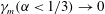
We conclude by noting that the Sweet–Parker current sheet in the presence of viscosity is instead thicker with respect to the inviscid case,
 $a_{SP}/L=S^{-1/2}(1+P)^{1/4}$
(Park, Monticello & White Reference Park, Monticello and White1984), whose inverse aspect ratio is indicated by the coloured stars in figure 6. Therefore, for large Prandtl numbers,
$a_{SP}/L=S^{-1/2}(1+P)^{1/4}$
(Park, Monticello & White Reference Park, Monticello and White1984), whose inverse aspect ratio is indicated by the coloured stars in figure 6. Therefore, for large Prandtl numbers,
 $P\geqslant S^{2/5}$
, the SP sheet can be quasi-stable to the tearing mode.
$P\geqslant S^{2/5}$
, the SP sheet can be quasi-stable to the tearing mode.

Figure 6. Growth rate normalized to the Alfvén time versus inverse aspect ratio at different Prandtl numbers. Stars correspond to the inverse aspect ratio of the viscous Sweet–Parker (from Tenerani et al. Reference Tenerani, Rappazzo, Velli and Pucci2015a ).
3.3 Collisionless reconnection in the ideal regime
In low-collision regimes where resistivity is effectively negligible, the dominant effects violating the ideal Ohm’s law are electron inertia and/or anisotropic electron pressure tensors. While both can allow magnetic reconnection, the latter usually requires a kinetic model (Cai & Lee Reference Cai and Lee1997; Scudder et al.
Reference Scudder, Karimabadi, Daughton and Roytershteyn2014), so the electron skin depth
 $d_{e}\equiv c/\unicode[STIX]{x1D714}_{pe}\propto \sqrt{m_{e}}$
often appears as the only non-ideal term driving collisionless tearing modes when a fluid description of the plasma is adopted. In this case, the small parameter is not
$d_{e}\equiv c/\unicode[STIX]{x1D714}_{pe}\propto \sqrt{m_{e}}$
often appears as the only non-ideal term driving collisionless tearing modes when a fluid description of the plasma is adopted. In this case, the small parameter is not
 $S^{-1}$
but rather the normalized electron skin depth
$S^{-1}$
but rather the normalized electron skin depth
 $d_{e}/L$
.
$d_{e}/L$
.
As a first step, we have considered the regime in which magnetic reconnection is induced by electron inertia in the strong guide field limit. The latter can be described by the Reduced MHD model in which the Hall term in Ohm’s law can be neglected to the lowest order (Strauss Reference Strauss1976; Schep, Pegoraro & Kuvshinov Reference Schep, Pegoraro and Kuvshinov1994; Del Sarto, Califano & Pegoraro Reference Del Sarto, Califano and Pegoraro2006). This description is suited, for instance, for tokamak and magnetically confined plasmas at low-
 $\unicode[STIX]{x1D6FD}$
, where
$\unicode[STIX]{x1D6FD}$
, where
 $\unicode[STIX]{x1D6FD}=8\unicode[STIX]{x03C0}P/B^{2}$
is the thermal to magnetic pressure ratio. It has been shown by Del Sarto et al. (Reference Del Sarto, Pucci, Tenerani and Velli2016) that in this regime the wave vector and growth rate of the fastest growing mode scale with the system parameters as
$\unicode[STIX]{x1D6FD}=8\unicode[STIX]{x03C0}P/B^{2}$
is the thermal to magnetic pressure ratio. It has been shown by Del Sarto et al. (Reference Del Sarto, Pucci, Tenerani and Velli2016) that in this regime the wave vector and growth rate of the fastest growing mode scale with the system parameters as
 $$\begin{eqnarray}k_{m}a\sim \frac{d_{e}}{a},\quad \unicode[STIX]{x1D6FE}_{m}\unicode[STIX]{x1D70F}_{A}\sim \left(\frac{d_{e}}{L}\right)^{2}\left(\frac{L}{a}\right)^{3},\quad \frac{\unicode[STIX]{x1D6FF}_{m}}{a}\sim \frac{d_{e}}{a}.\end{eqnarray}$$
From the scaling of the maximum growth rate
 $\unicode[STIX]{x1D6FE}_{m}\unicode[STIX]{x1D70F}_{A}$
in (3.6) it follows that onset of ‘ideal’ reconnection, that is when the growth rate becomes independent of the small non-ideal parameter
$\unicode[STIX]{x1D6FE}_{m}\unicode[STIX]{x1D70F}_{A}$
in (3.6) it follows that onset of ‘ideal’ reconnection, that is when the growth rate becomes independent of the small non-ideal parameter
 $d_{e}/L$
, occurs once a critical aspect ratio
$d_{e}/L$
, occurs once a critical aspect ratio
 $$\begin{eqnarray}\frac{a_{i}}{L}\sim \left(\frac{d_{e}}{L}\right)^{2/3}\end{eqnarray}$$
is reached. In the limit of strong guide field it is possible to retain also some kinetic corrections related to electron temperature anisotropies and ion finite-Larmor-radius (FLR) effects in a simple way (Schep et al.
Reference Schep, Pegoraro and Kuvshinov1994; Waelbroeck, Hazeltine & Morrison Reference Waelbroeck, Hazeltine and Morrison2009), that can be included in the reduced MHD model when approximated to their dominant gyrotropic contribution (we then speak of gyrofluid models). These models can be used also at relatively large
 $\unicode[STIX]{x1D6FD}$
values (Grasso, Tassi & Waelbroeck Reference Grasso, Tassi and Waelbroeck2010). Electron temperature effects arise at length scales of the order of the ion sound Larmor radius
$\unicode[STIX]{x1D6FD}$
values (Grasso, Tassi & Waelbroeck Reference Grasso, Tassi and Waelbroeck2010). Electron temperature effects arise at length scales of the order of the ion sound Larmor radius
 $\unicode[STIX]{x1D70C}_{s}=c_{s}/\unicode[STIX]{x1D6FA}_{i}$
,
$\unicode[STIX]{x1D70C}_{s}=c_{s}/\unicode[STIX]{x1D6FA}_{i}$
,
 $c_{s}=\sqrt{T_{e}/m_{i}}$
being the ion sound speed and
$c_{s}=\sqrt{T_{e}/m_{i}}$
being the ion sound speed and
 $\unicode[STIX]{x1D6FA}_{i}$
the ion cyclotron frequency. These additional terms in the generalized Ohm’s law can be seen as the result of an anisotropic electron pressure contribution (Schep et al.
Reference Schep, Pegoraro and Kuvshinov1994), or as the Hall term contribution when the diamagnetic drift is retained as a first-order correction to the
$\unicode[STIX]{x1D6FA}_{i}$
the ion cyclotron frequency. These additional terms in the generalized Ohm’s law can be seen as the result of an anisotropic electron pressure contribution (Schep et al.
Reference Schep, Pegoraro and Kuvshinov1994), or as the Hall term contribution when the diamagnetic drift is retained as a first-order correction to the
 $\boldsymbol{E}\times \boldsymbol{B}$
electron drift (see also Del Sarto et al.
Reference Del Sarto, Pucci, Tenerani and Velli2016). Ion FLR effects introduce as a further length scale the ion Larmor radius
$\boldsymbol{E}\times \boldsymbol{B}$
electron drift (see also Del Sarto et al.
Reference Del Sarto, Pucci, Tenerani and Velli2016). Ion FLR effects introduce as a further length scale the ion Larmor radius
 $\unicode[STIX]{x1D70C}_{i}=v_{th}^{i}/\unicode[STIX]{x1D6FA}_{i}$
, where
$\unicode[STIX]{x1D70C}_{i}=v_{th}^{i}/\unicode[STIX]{x1D6FA}_{i}$
, where
 $v_{th}^{i}$
is the ion thermal speed. Depending on the way ion FLR are approximated from kinetic theory, different gyrofluid models can be obtained, all yielding the same dispersion relation for finite temperature tearing instabilities when
$v_{th}^{i}$
is the ion thermal speed. Depending on the way ion FLR are approximated from kinetic theory, different gyrofluid models can be obtained, all yielding the same dispersion relation for finite temperature tearing instabilities when
 $\unicode[STIX]{x1D70C}_{\unicode[STIX]{x1D70F}}^{2}\equiv \unicode[STIX]{x1D70C}_{s}^{2}+\unicode[STIX]{x1D70C}_{i}^{2}\gg d_{e}^{2}$
(Pegoraro & Schep Reference Pegoraro and Schep1986; Porcelli Reference Porcelli1991; Ottaviani & Porcelli Reference Ottaviani and Porcelli1995). An explicit expression for the fastest growing mode valid in this regime can be found in Comisso et al. (Reference Comisso, Grasso, Waelbroeck and Borgogno2013). For a Harris sheet, when rescaled from the sheet thickness
$\unicode[STIX]{x1D70C}_{\unicode[STIX]{x1D70F}}^{2}\equiv \unicode[STIX]{x1D70C}_{s}^{2}+\unicode[STIX]{x1D70C}_{i}^{2}\gg d_{e}^{2}$
(Pegoraro & Schep Reference Pegoraro and Schep1986; Porcelli Reference Porcelli1991; Ottaviani & Porcelli Reference Ottaviani and Porcelli1995). An explicit expression for the fastest growing mode valid in this regime can be found in Comisso et al. (Reference Comisso, Grasso, Waelbroeck and Borgogno2013). For a Harris sheet, when rescaled from the sheet thickness
 $a$
to the length
$a$
to the length
 $L$
, the wavenumber and growth rate of the fastest growing mode are therefore the following (Del Sarto et al.
Reference Del Sarto, Pucci, Tenerani and Velli2016),
$L$
, the wavenumber and growth rate of the fastest growing mode are therefore the following (Del Sarto et al.
Reference Del Sarto, Pucci, Tenerani and Velli2016),
 $$\begin{eqnarray}k_{m}a\sim \frac{d_{e}}{L}\left(\frac{\unicode[STIX]{x1D70C}_{\unicode[STIX]{x1D70F}}}{d_{e}}\right)^{1/3}\frac{L}{a},\quad \unicode[STIX]{x1D6FE}_{m}\unicode[STIX]{x1D70F}_{A}\sim \left(\frac{d_{e}}{L}\right)^{2}\frac{\unicode[STIX]{x1D70C}_{\unicode[STIX]{x1D70F}}}{d_{e}}\left(\frac{L}{a}\right)^{3}\quad (\unicode[STIX]{x1D70C}_{\unicode[STIX]{x1D70F}}\gg d_{e}).\end{eqnarray}$$
In this regime, the critical inverse aspect ratio scales with both
 $d_{e}/L$
and
$d_{e}/L$
and
 $\unicode[STIX]{x1D70C}_{\unicode[STIX]{x1D70F}}/d_{e}$
as
$\unicode[STIX]{x1D70C}_{\unicode[STIX]{x1D70F}}/d_{e}$
as
 $$\begin{eqnarray}\frac{a_{i}}{L}\sim \left(\frac{d_{e}}{L}\right)^{2/3}\left(\frac{\unicode[STIX]{x1D70C}_{\unicode[STIX]{x1D70F}}}{d_{e}}\right)^{1/3}\quad (\unicode[STIX]{x1D70C}_{\unicode[STIX]{x1D70F}}\gg d_{e}).\end{eqnarray}$$
In conclusion, kinetic effects increase the linear growth rate by a factor
 $\unicode[STIX]{x1D70C}_{\unicode[STIX]{x1D70F}}/d_{e}$
with respect to the low-
$\unicode[STIX]{x1D70C}_{\unicode[STIX]{x1D70F}}/d_{e}$
with respect to the low-
 $\unicode[STIX]{x1D6FD}$
case, as can be seen by comparing the growth rate in (3.6) with the one including finite temperature effects in (3.8). As a consequence, the critical inverse aspect ratio turns out to be thicker in the latter case by a factor scaling as
$\unicode[STIX]{x1D6FD}$
case, as can be seen by comparing the growth rate in (3.6) with the one including finite temperature effects in (3.8). As a consequence, the critical inverse aspect ratio turns out to be thicker in the latter case by a factor scaling as
 $(\unicode[STIX]{x1D70C}_{\unicode[STIX]{x1D70F}}/d_{e})^{1/3}$
(cf. (3.7) and (3.9)).
$(\unicode[STIX]{x1D70C}_{\unicode[STIX]{x1D70F}}/d_{e})^{1/3}$
(cf. (3.7) and (3.9)).
4 The trigger problem
Observations show that many explosive phenomena usually display an initial phase (of long but uncertain duration) during which energy is transferred to and accumulated in the system in question, followed by an abrupt destabilization process expressed by an impulsive phase, often attributed to the onset, or trigger, of magnetic reconnection. During the impulsive phase energy is suddenly released on a fast (ideal) time scale (of the order of a few
 $\unicode[STIX]{x1D70F}_{A}$
) in the form of heat, kinetic energy and populations of accelerated particles. The impulsive phase is followed by main and recovery phases, whereby energy released becomes more gradual and the system relaxes towards a quiet configuration (Akasofu Reference Akasofu1964; Wesson Reference Wesson1986; Fletcher et al.
Reference Fletcher, Dennis, Hudson and Krucker2011). Solar flares provide one of the most spectacular examples in this sense: a prominence can stand for weeks in the solar corona until it erupts by releasing a huge amount of energy (the flare), of about
$\unicode[STIX]{x1D70F}_{A}$
) in the form of heat, kinetic energy and populations of accelerated particles. The impulsive phase is followed by main and recovery phases, whereby energy released becomes more gradual and the system relaxes towards a quiet configuration (Akasofu Reference Akasofu1964; Wesson Reference Wesson1986; Fletcher et al.
Reference Fletcher, Dennis, Hudson and Krucker2011). Solar flares provide one of the most spectacular examples in this sense: a prominence can stand for weeks in the solar corona until it erupts by releasing a huge amount of energy (the flare), of about
 $10^{30}-10^{32}$
erg, in a few tens of minutes or hours, depending on their size. The flare displays an impulsive phase, that can be seen as sudden intensity enhancements in different wavelengths, especially in the hard X-ray spectrum, lasting usually no more than a few minutes for the larger events (Ellison Reference Ellison1946; Kane Reference Kane1974; Ajello et al.
Reference Ajello, Albert, Allafort, Baldini, Barbiellini, Bastieri, Bellazzini, Bissaldi, Bonamente and Brandt2014).
$10^{30}-10^{32}$
erg, in a few tens of minutes or hours, depending on their size. The flare displays an impulsive phase, that can be seen as sudden intensity enhancements in different wavelengths, especially in the hard X-ray spectrum, lasting usually no more than a few minutes for the larger events (Ellison Reference Ellison1946; Kane Reference Kane1974; Ajello et al.
Reference Ajello, Albert, Allafort, Baldini, Barbiellini, Bastieri, Bellazzini, Bissaldi, Bonamente and Brandt2014).
In the weakly collisional plasmas found in many astrophysical environments, or in fusion devices, bulk plasma motions tend to form thin current sheets spontaneously in localized regions (Syrovatskiǐ Reference Syrovatskiǐ1971; Biskamp Reference Biskamp1993). There, the intense currents are limited only by the extremely small resistivity or by other effects, such as electron inertia, until they ultimately relax once reconnection is enabled inside these thin boundary layers. The problem of understanding in which way thin current sheets form is a complex and rich one, both theoretically and numerically. We therefore do not go into details, but some recent studies about thin current sheet formation for configurations relevant to magnetosphere dynamics and the solar corona can be found for instance in Birn & Schindler (Reference Birn and Schindler2002), Titov, Galsgaard & Neukirch (Reference Titov, Galsgaard and Neukirch2003), Aulanier, Pariat & Démoulin (Reference Aulanier, Pariat and Démoulin2005), Rappazzo & Parker (Reference Rappazzo and Parker2013), Hsieh & Otto (Reference Hsieh and Otto2015).
Whatever the mechanism might be, one can always imagine that, during current sheet formation, the system evolves through a sequence of similar configurations to which the linear stability analysis can be applied in order to investigate its properties. As shown in § 3, the growth rate of the reconnecting tearing mode instability exhibits a strong dependence on the current sheet aspect ratio, for example in resistive MHD
 $\unicode[STIX]{x1D6FE}\unicode[STIX]{x1D70F}_{A}\propto (L/a)^{3/2}$
(cf. (3.1)). This, together with the large values of the Lundquist number, or
$\unicode[STIX]{x1D6FE}\unicode[STIX]{x1D70F}_{A}\propto (L/a)^{3/2}$
(cf. (3.1)). This, together with the large values of the Lundquist number, or
 $L/d_{e}$
, suggests that the formation of small scales all the way down to the critical thickness would naturally lead to the trigger of fast reconnection.
$L/d_{e}$
, suggests that the formation of small scales all the way down to the critical thickness would naturally lead to the trigger of fast reconnection.
4.1 Scenario
In the following, we will assume a current profile that thins exponentially in time. Exponentially thinning current sheets are indeed of particular importance, as they are commonly observed in simulations of solar and stellar coronal heating (Rappazzo & Parker Reference Rappazzo and Parker2013), as self-similar solutions of X-point collapse (Sulem et al. Reference Sulem, Frisch, Pouquet and Meneguzzi1985), as well as in in situ measurements during the growth phase of substorms in the Earth’s magnetotail (Sanny et al. Reference Sanny, McPherron, Russel, Baker, Pulkkinen and Nishida1994), to give some examples.
We therefore assume that the ambient plasma and magnetic fields evolve over a time scale
 $\unicode[STIX]{x1D70F}_{c}$
which is determined by ideal plasma motions and hence does not depend on
$\unicode[STIX]{x1D70F}_{c}$
which is determined by ideal plasma motions and hence does not depend on
 $S$
. Consider the simpler case of resistive (incompressible) MHD, and take a Harris current sheet of inverse aspect ratio
$S$
. Consider the simpler case of resistive (incompressible) MHD, and take a Harris current sheet of inverse aspect ratio
 $a/L$
shrinking on a time scale
$a/L$
shrinking on a time scale
 $\unicode[STIX]{x1D70F}_{c}\sim a\,(\text{d}a/\text{d}t)^{-1}\gtrsim \unicode[STIX]{x1D70F}_{A}$
. The parameter
$\unicode[STIX]{x1D70F}_{c}\sim a\,(\text{d}a/\text{d}t)^{-1}\gtrsim \unicode[STIX]{x1D70F}_{A}$
. The parameter
 $\unicode[STIX]{x1D70F}_{c}$
thus represents schematically the coupling between the local dynamics within the current sheet and some external process inducing the thinning itself. Within this framework, we extend the tearing mode analysis to systems that are parameterized in time through the evolving aspect ratio (Tenerani et al.
Reference Tenerani, Velli, Rappazzo and Pucci2015b
).
$\unicode[STIX]{x1D70F}_{c}$
thus represents schematically the coupling between the local dynamics within the current sheet and some external process inducing the thinning itself. Within this framework, we extend the tearing mode analysis to systems that are parameterized in time through the evolving aspect ratio (Tenerani et al.
Reference Tenerani, Velli, Rappazzo and Pucci2015b
).
An investigation of the disruption of a forming current sheet germane to the present discussion has been recently published in Uzdensky & Loureiro (Reference Uzdensky and Loureiro2016). Since the two scenarios differ somewhat, let us briefly comment on the differences here, although we refer to that paper for more details. Our study focuses on the linear stage of the tearing instability to provide a possible explanation for the onset of fast reconnection, using a WKB approach to describe the growth of unstable modes during the dynamical collapse of the sheet. In this way, we take into account that unstable modes with a growth rate exceeding
 $\unicode[STIX]{x1D70F}_{c}^{-1}$
can in principle compete in disrupting the current sheet. Uzdensky & Loureiro (Reference Uzdensky and Loureiro2016), on the other hand, consider arbitrary time scales for driving the sheet collapse, and start from the assumption that the linear stage of a mode ends once its growth rate exceeds the driving rate. They then estimate that the first mode to meet this condition will also be the one dominating the subsequent nonlinear evolution. They therefore examine the nonlinear regime to describe the disruption of the current sheet, which in their scenario may occur also on time scales scaling as a positive power of
$\unicode[STIX]{x1D70F}_{c}^{-1}$
can in principle compete in disrupting the current sheet. Uzdensky & Loureiro (Reference Uzdensky and Loureiro2016), on the other hand, consider arbitrary time scales for driving the sheet collapse, and start from the assumption that the linear stage of a mode ends once its growth rate exceeds the driving rate. They then estimate that the first mode to meet this condition will also be the one dominating the subsequent nonlinear evolution. They therefore examine the nonlinear regime to describe the disruption of the current sheet, which in their scenario may occur also on time scales scaling as a positive power of
 $S$
. In this sense, they do not impose restrictions on mode growth times with respect to dissipative coefficients. Our approach on the other hand focuses precisely on the latter aspect, our framework being one in which things will occur on the fastest possible times compatible with the dynamical system in question, and therefore, in analogy for example with turbulence, we expect the fastest growing modes not to scale with the dissipative coefficients. So in some sense the approach of Uzdensky & Loureiro (Reference Uzdensky and Loureiro2016) is more general than ours, but does not investigate in detail whether and under which conditions the transition to fast reconnection (the trigger) might occur. Other recent interesting analyses of a similar conceptual reconnection problem, the Taylor’s problem, have been provided by Comisso, Grasso & Waelbroeck (Reference Comisso, Grasso and Waelbroeck2015) and Vekstein & Kusano (Reference Vekstein and Kusano2015). They analyse the possible time evolution of an initial macroscopic, stable current layer which is subject to a finite-amplitude perturbation at its boundaries, and recognize the role sufficiently fast tearing modes may play in disrupting the current sheet. We do not discuss that problem here, although it would be interesting to study how in the asymptotic limit of large
$S$
. In this sense, they do not impose restrictions on mode growth times with respect to dissipative coefficients. Our approach on the other hand focuses precisely on the latter aspect, our framework being one in which things will occur on the fastest possible times compatible with the dynamical system in question, and therefore, in analogy for example with turbulence, we expect the fastest growing modes not to scale with the dissipative coefficients. So in some sense the approach of Uzdensky & Loureiro (Reference Uzdensky and Loureiro2016) is more general than ours, but does not investigate in detail whether and under which conditions the transition to fast reconnection (the trigger) might occur. Other recent interesting analyses of a similar conceptual reconnection problem, the Taylor’s problem, have been provided by Comisso, Grasso & Waelbroeck (Reference Comisso, Grasso and Waelbroeck2015) and Vekstein & Kusano (Reference Vekstein and Kusano2015). They analyse the possible time evolution of an initial macroscopic, stable current layer which is subject to a finite-amplitude perturbation at its boundaries, and recognize the role sufficiently fast tearing modes may play in disrupting the current sheet. We do not discuss that problem here, although it would be interesting to study how in the asymptotic limit of large
 $S$
the ‘ideal’ tearing framework affects those models. Let us focus now on our scenario of an exponentially thinning sheet.
$S$
the ‘ideal’ tearing framework affects those models. Let us focus now on our scenario of an exponentially thinning sheet.
On the basis of the rescaling argument, the growth rates in the small and large
 $\unicode[STIX]{x1D6E5}^{\prime }$
regimes discussed in § 2 can now be generalized to arbitrary aspect ratios. By taking
$\unicode[STIX]{x1D6E5}^{\prime }$
regimes discussed in § 2 can now be generalized to arbitrary aspect ratios. By taking
 $\unicode[STIX]{x1D6E5}^{\prime }a\sim [(ka)^{-1}-ka]$
for a Harris sheet, these are given, respectively, by
$\unicode[STIX]{x1D6E5}^{\prime }a\sim [(ka)^{-1}-ka]$
for a Harris sheet, these are given, respectively, by
 $$\begin{eqnarray}\unicode[STIX]{x1D6FE}\unicode[STIX]{x1D70F}_{A}\sim S^{-3/5}\left(\frac{a}{L}\right)^{-8/5}(ka)^{-2/5}[1-(ka)^{2}]^{4/5},\quad \unicode[STIX]{x1D6FE}\unicode[STIX]{x1D70F}_{A}\sim S^{-1/3}\left(\frac{a}{L}\right)^{-2}(ka)^{2/3}.\end{eqnarray}$$
The fastest growing mode, as already shown in § 3, has the growth rate scaling as
 $$\begin{eqnarray}\unicode[STIX]{x1D6FE}_{m}\unicode[STIX]{x1D70F}_{A}\sim S^{-1/2}\left(\frac{a}{L}\right)^{-3/2},\end{eqnarray}$$
whereas the wave vector and thickness of inner diffusion layer scale, respectively, as
 $$\begin{eqnarray}k_{m}a\sim S^{-1/4}\left(\frac{a}{L}\right)^{-1/4},\quad \frac{\unicode[STIX]{x1D6FF}_{m}}{a}\sim S^{-1/4}\left(\frac{a}{L}\right)^{-1/4}.\end{eqnarray}$$
As the thinning proceeds in time, modes with increasing wave vector
 $k$
are progressively destabilized, owing to the traditional instability condition
$k$
are progressively destabilized, owing to the traditional instability condition
 $ka(t)<1$
in a Harris sheet. In this way, each newly destabilized mode lies in the small
$ka(t)<1$
in a Harris sheet. In this way, each newly destabilized mode lies in the small
 $\unicode[STIX]{x1D6E5}^{\prime }$
regime and it transitions toward the large
$\unicode[STIX]{x1D6E5}^{\prime }$
regime and it transitions toward the large
 $\unicode[STIX]{x1D6E5}^{\prime }$
one as time elapses, by crossing at some point the fastest growing mode. This can be understood also by looking back at the plot in figure 4: since
$\unicode[STIX]{x1D6E5}^{\prime }$
one as time elapses, by crossing at some point the fastest growing mode. This can be understood also by looking back at the plot in figure 4: since
 $\bar{S}\equiv S(a/L)$
, if
$\bar{S}\equiv S(a/L)$
, if
 $a/L$
decreases at fixed
$a/L$
decreases at fixed
 $S$
, then
$S$
, then
 $\bar{S}$
decreases accordingly, so that a given mode shifts from the right to left side of the plot. On the other hand, only those modes fitting within the current sheet, that therefore satisfy
$\bar{S}$
decreases accordingly, so that a given mode shifts from the right to left side of the plot. On the other hand, only those modes fitting within the current sheet, that therefore satisfy
 $kL\geqslant 2\unicode[STIX]{x03C0}$
, can grow. This implies that at the beginning, when
$kL\geqslant 2\unicode[STIX]{x03C0}$
, can grow. This implies that at the beginning, when
 $a\lesssim L$
, there are only unstable modes in the small
$a\lesssim L$
, there are only unstable modes in the small
 $\unicode[STIX]{x1D6E5}^{\prime }$
regime. This initial stage in turn ends when the smallest unstable mode, which has a wavelength of the order of the current sheet length
$\unicode[STIX]{x1D6E5}^{\prime }$
regime. This initial stage in turn ends when the smallest unstable mode, which has a wavelength of the order of the current sheet length
 $L$
,
$L$
,
 $k\sim 2\unicode[STIX]{x03C0}/L$
, coincides with
$k\sim 2\unicode[STIX]{x03C0}/L$
, coincides with
 $k_{m}$
(Uzdensky & Loureiro Reference Uzdensky and Loureiro2016). This happens when
$k_{m}$
(Uzdensky & Loureiro Reference Uzdensky and Loureiro2016). This happens when
 $S^{-1/4}(a/L)^{-1/4}\simeq 2\unicode[STIX]{x03C0}(a/L)$
, or, in other words, when
$S^{-1/4}(a/L)^{-1/4}\simeq 2\unicode[STIX]{x03C0}(a/L)$
, or, in other words, when
 $a/L\lesssim 0.2S^{-1/5}$
. At that point, the fastest growing mode will be always unstable, and hence it will dominate over both the small and the large
$a/L\lesssim 0.2S^{-1/5}$
. At that point, the fastest growing mode will be always unstable, and hence it will dominate over both the small and the large
 $\unicode[STIX]{x1D6E5}^{\prime }$
modes. The initial stage evolving in the small
$\unicode[STIX]{x1D6E5}^{\prime }$
modes. The initial stage evolving in the small
 $\unicode[STIX]{x1D6E5}^{\prime }$
regime however does not contribute significantly to the growth of perturbations so one can consider only the regime given by the fastest growing mode, expressed by (4.2)–(4.3), to describe the transition to fast reconnection. Indeed, the small
$\unicode[STIX]{x1D6E5}^{\prime }$
regime however does not contribute significantly to the growth of perturbations so one can consider only the regime given by the fastest growing mode, expressed by (4.2)–(4.3), to describe the transition to fast reconnection. Indeed, the small
 $\unicode[STIX]{x1D6E5}^{\prime }$
(as well as the large
$\unicode[STIX]{x1D6E5}^{\prime }$
(as well as the large
 $\unicode[STIX]{x1D6E5}^{\prime }$
) regime has a growth rate that, even if the current sheet is thinning, goes to zero for
$\unicode[STIX]{x1D6E5}^{\prime }$
) regime has a growth rate that, even if the current sheet is thinning, goes to zero for
 $S\rightarrow \infty$
(according to (4.1)). As a consequence, modes in that regime cannot grow during a finite interval of time of order of
$S\rightarrow \infty$
(according to (4.1)). As a consequence, modes in that regime cannot grow during a finite interval of time of order of
 $\unicode[STIX]{x1D70F}_{c}$
. In other words, the small
$\unicode[STIX]{x1D70F}_{c}$
. In other words, the small
 $\unicode[STIX]{x1D6E5}^{\prime }$
regime corresponds to slow reconnection and it cannot in general provide the transition to fast reconnection in quasi-ideal plasmas. Assuming a collapse of the form
$\unicode[STIX]{x1D6E5}^{\prime }$
regime corresponds to slow reconnection and it cannot in general provide the transition to fast reconnection in quasi-ideal plasmas. Assuming a collapse of the form
 $a(t)=\exp (-t/\unicode[STIX]{x1D70F}_{c})$
, which can be easily generalized to include an exponential increase of the length
$a(t)=\exp (-t/\unicode[STIX]{x1D70F}_{c})$
, which can be easily generalized to include an exponential increase of the length
 $L$
, then the amplitude of the reconnecting magnetic flux
$L$
, then the amplitude of the reconnecting magnetic flux
 $\unicode[STIX]{x1D713}$
is given by
$\unicode[STIX]{x1D713}$
is given by
 $$\begin{eqnarray}\unicode[STIX]{x1D713}(t)=\unicode[STIX]{x1D713}(0)\exp \left(\int _{0}^{t}\unicode[STIX]{x1D6FE}(t^{\prime })\,\text{d}t^{\prime }\right),\end{eqnarray}$$
where, by neglecting the initial small
 $\unicode[STIX]{x1D6E5}^{\prime }$
stage (current sheets having
$\unicode[STIX]{x1D6E5}^{\prime }$
stage (current sheets having
 $a/L>S^{-1/5}$
), the integrand is given by
$a/L>S^{-1/5}$
), the integrand is given by
 $$\begin{eqnarray}\unicode[STIX]{x1D6FE}(t)=\unicode[STIX]{x1D6FE}_{m}(t)=\frac{1}{\unicode[STIX]{x1D70F}_{A}}\,0.63\,S^{-1/2}\left[\exp \left(\frac{t}{\unicode[STIX]{x1D70F}_{c}}\right)\right]^{3/2}.\end{eqnarray}$$
 $$\begin{eqnarray}\unicode[STIX]{x1D713}(t)=\unicode[STIX]{x1D713}(0)\exp \left[\frac{2\unicode[STIX]{x1D70F}_{c}}{3}0.63\,S^{-1/2}(\text{e}^{3t/(2\unicode[STIX]{x1D70F}_{c})}-1)\right],\end{eqnarray}$$
that can be approximated as follows,
 $$\begin{eqnarray}\displaystyle & \displaystyle \unicode[STIX]{x1D713}(t)\simeq \unicode[STIX]{x1D713}(0)\text{e}^{\unicode[STIX]{x1D6FE}_{m}(0)t},\quad \text{if }t\ll \unicode[STIX]{x1D70F}_{c}\,2/3, & \displaystyle\end{eqnarray}$$
 $$\begin{eqnarray}\displaystyle & \displaystyle \unicode[STIX]{x1D713}(t)\simeq \unicode[STIX]{x1D713}(0)\text{e}^{\unicode[STIX]{x1D6FE}_{m}(t)2\unicode[STIX]{x1D70F}_{c}/3},\quad \text{if }t>\unicode[STIX]{x1D70F}_{c}\,2/3. & \displaystyle\end{eqnarray}$$
The onset of the tearing instability roughly takes place when unstable modes have time to develop, hence at about the time
 $\unicode[STIX]{x1D70F}_{\ast }$
such that
$\unicode[STIX]{x1D70F}_{\ast }$
such that
 $\unicode[STIX]{x1D6FE}_{m}(\unicode[STIX]{x1D70F}_{\ast })\unicode[STIX]{x1D70F}_{c}\simeq 1$
, as can be seen also from (4.8). In turn, the growth rate rapidly increases while approaching the critical thickness
$\unicode[STIX]{x1D6FE}_{m}(\unicode[STIX]{x1D70F}_{\ast })\unicode[STIX]{x1D70F}_{c}\simeq 1$
, as can be seen also from (4.8). In turn, the growth rate rapidly increases while approaching the critical thickness
 $a_{i}/L\sim S^{-1/3}$
from above, so one can easily be convinced that a fast current sheet collapse naturally drives an explosive transition from a quasi-stable state – growth rate depending on a negative power of
$a_{i}/L\sim S^{-1/3}$
from above, so one can easily be convinced that a fast current sheet collapse naturally drives an explosive transition from a quasi-stable state – growth rate depending on a negative power of
 $S$
– to an ideally unstable one.
$S$
– to an ideally unstable one.

Figure 7. Temporal evolution of a thinning Harris current sheet. The out-of-plane current density
 $j_{z}$
is colour coded and white lines represent magnetic field lines.
$j_{z}$
is colour coded and white lines represent magnetic field lines.

Figure 8. Temporal evolution of the current sheet thickness (a) and of the amplitude of some Fourier modes of the flux function
 $\unicode[STIX]{x1D713}$
at the neutral line (b) of the simulation shown in figure 7. The dashed line corresponds to the integral given in (4.4) where the functional form
$\unicode[STIX]{x1D713}$
at the neutral line (b) of the simulation shown in figure 7. The dashed line corresponds to the integral given in (4.4) where the functional form
 $a(t)$
adopted in the simulation (see text) has been used (from Tenerani et al.
Reference Tenerani, Velli, Rappazzo and Pucci2015b
).
$a(t)$
adopted in the simulation (see text) has been used (from Tenerani et al.
Reference Tenerani, Velli, Rappazzo and Pucci2015b
).
We have tested such scenario with fully nonlinear MHD simulations in which a collapse of the current sheet is imposed a priori with
 $\unicode[STIX]{x1D70F}_{c}$
in the range
$\unicode[STIX]{x1D70F}_{c}$
in the range
 $1-10\,\unicode[STIX]{x1D70F}_{A}$
(Tenerani et al.
Reference Tenerani, Velli, Rappazzo and Pucci2015b
). Figure 7 shows an example of the temporal evolution of an exponentially thinning Harris sheet initially perturbed by a random noise of fluctuations. The Lundquist number in these simulations is set to
$1-10\,\unicode[STIX]{x1D70F}_{A}$
(Tenerani et al.
Reference Tenerani, Velli, Rappazzo and Pucci2015b
). Figure 7 shows an example of the temporal evolution of an exponentially thinning Harris sheet initially perturbed by a random noise of fluctuations. The Lundquist number in these simulations is set to
 $S=10^{6}$
and the Prandtl number to
$S=10^{6}$
and the Prandtl number to
 $P=1$
, so that the scalings of the non-viscous case are not modified significantly. The in-plane magnetic field is
$P=1$
, so that the scalings of the non-viscous case are not modified significantly. The in-plane magnetic field is
 $\boldsymbol{B}=B_{0}\tanh [y/a(t)]\hat{\boldsymbol{x}}$
and, for numerical convenience, a thinning of the form
$\boldsymbol{B}=B_{0}\tanh [y/a(t)]\hat{\boldsymbol{x}}$
and, for numerical convenience, a thinning of the form
 $a(t)=a_{0}\exp (-t/\unicode[STIX]{x1D70F}_{c})+a_{\infty }(1-\exp (-t/\unicode[STIX]{x1D70F}_{c}))$
has been chosen. For the case shown in figure 7 we have fixed
$a(t)=a_{0}\exp (-t/\unicode[STIX]{x1D70F}_{c})+a_{\infty }(1-\exp (-t/\unicode[STIX]{x1D70F}_{c}))$
has been chosen. For the case shown in figure 7 we have fixed
 $a_{\infty }/a_{0}=0.1$
, with
$a_{\infty }/a_{0}=0.1$
, with
 $a_{0}=0.1\,L$
and
$a_{0}=0.1\,L$
and
 $\unicode[STIX]{x1D70F}_{c}=4\,\unicode[STIX]{x1D70F}_{A}$
. In figure 8 we show the temporal evolution of
$\unicode[STIX]{x1D70F}_{c}=4\,\unicode[STIX]{x1D70F}_{A}$
. In figure 8 we show the temporal evolution of
 $a(t)$
(a) and of some unstable Fourier modes of
$a(t)$
(a) and of some unstable Fourier modes of
 $\unicode[STIX]{x1D713}$
at the neutral line
$\unicode[STIX]{x1D713}$
at the neutral line
 $y=0$
(b) for the same simulation. The simulation illustrates that during the linear stage of the instability (from
$y=0$
(b) for the same simulation. The simulation illustrates that during the linear stage of the instability (from
 $t\simeq 11$
to
$t\simeq 11$
to
 $t\simeq 22$
 $\unicode[STIX]{x1D70F}_{A}$
) the magnetic field rapidly reconnects in a few Alfvén times when the critical thickness
$\unicode[STIX]{x1D70F}_{A}$
) the magnetic field rapidly reconnects in a few Alfvén times when the critical thickness
 $a_{i}/L\sim S^{-1/3}\simeq 0.01$
is approached from above, and that the current breaks up into a number of magnetic islands
$a_{i}/L\sim S^{-1/3}\simeq 0.01$
is approached from above, and that the current breaks up into a number of magnetic islands
 $N_{i}$
that scales as
$N_{i}$
that scales as
 $N_{i}\sim S^{1/6}\simeq 10$
. As can be seen from figure 7, the following nonlinear stage is characterized by the competition between coalescence of magnetic islands (this can be seen also by looking at the increasing magnitude of long-wavelength modes,
$N_{i}\sim S^{1/6}\simeq 10$
. As can be seen from figure 7, the following nonlinear stage is characterized by the competition between coalescence of magnetic islands (this can be seen also by looking at the increasing magnitude of long-wavelength modes,
 $kL=5$
and
$kL=5$
and
 $kL=1$
, in figure 8) and X-point collapse, in a way qualitatively similar to that discussed in Malara, Veltri & Carbone (Reference Malara, Veltri and Carbone1992). We defer more detailed discussions about the nonlinear evolution of an ‘ideally’ reconnecting current sheet to § 5.
$kL=1$
, in figure 8) and X-point collapse, in a way qualitatively similar to that discussed in Malara, Veltri & Carbone (Reference Malara, Veltri and Carbone1992). We defer more detailed discussions about the nonlinear evolution of an ‘ideally’ reconnecting current sheet to § 5.
To summarize, in the scenario proposed above the mechanism driving the collapse (that can be mapped in the developmental phase, or the storage phase) is not specified. The ambient current sheet thins on a time scale
 $\unicode[STIX]{x1D70F}_{c}$
which is independent from
$\unicode[STIX]{x1D70F}_{c}$
which is independent from
 $S$
and instability is let to freely evolve from an initial slow phase of reconnection, when the thickness is larger than critical, to an ideally fast one while approaching the critical inverse aspect ratio
$S$
and instability is let to freely evolve from an initial slow phase of reconnection, when the thickness is larger than critical, to an ideally fast one while approaching the critical inverse aspect ratio
 $a_{i}/L\sim S^{-1/3}$
. Numerical simulations of a thinning current sheet with
$a_{i}/L\sim S^{-1/3}$
. Numerical simulations of a thinning current sheet with
 $\unicode[STIX]{x1D70F}_{c}\simeq 1-10\,\unicode[STIX]{x1D70F}_{A}$
show that when approaching the critical inverse aspect ratio from above magnetic islands significantly grow from the initial noise up to the thickness of the inner layer of the reconnecting current sheet itself and beyond, during the nonlinear stage, on a time scale of the order of a few
$\unicode[STIX]{x1D70F}_{c}\simeq 1-10\,\unicode[STIX]{x1D70F}_{A}$
show that when approaching the critical inverse aspect ratio from above magnetic islands significantly grow from the initial noise up to the thickness of the inner layer of the reconnecting current sheet itself and beyond, during the nonlinear stage, on a time scale of the order of a few
 $\unicode[STIX]{x1D70F}_{A}$
. In the model that we have chosen of an exponential collapse the time needed to form the ideally unstable current sheet is about
$\unicode[STIX]{x1D70F}_{A}$
. In the model that we have chosen of an exponential collapse the time needed to form the ideally unstable current sheet is about
 $\unicode[STIX]{x1D70F}_{i}\simeq (\unicode[STIX]{x1D70F}_{c}/3)\ln (S)$
, i.e. it depends very weakly (logarithmically) on
$\unicode[STIX]{x1D70F}_{i}\simeq (\unicode[STIX]{x1D70F}_{c}/3)\ln (S)$
, i.e. it depends very weakly (logarithmically) on
 $S$
and allows for a two time scale dynamics. For instance, if
$S$
and allows for a two time scale dynamics. For instance, if
 $\unicode[STIX]{x1D70F}_{c}=1{-}10\,\unicode[STIX]{x1D70F}_{A}$
and
$\unicode[STIX]{x1D70F}_{c}=1{-}10\,\unicode[STIX]{x1D70F}_{A}$
and
 $S=10^{12}{-}10^{14}$
then
$S=10^{12}{-}10^{14}$
then
 $\unicode[STIX]{x1D70F}_{i}\simeq 10{-}100\,\unicode[STIX]{x1D70F}_{A}$
thus one or two orders of magnitude larger than the time expected for the onset and development of ‘ideal’ reconnection.
$\unicode[STIX]{x1D70F}_{i}\simeq 10{-}100\,\unicode[STIX]{x1D70F}_{A}$
thus one or two orders of magnitude larger than the time expected for the onset and development of ‘ideal’ reconnection.
Nonlinearities become important when the half-width
 $w$
of magnetic islands, given approximately by
$w$
of magnetic islands, given approximately by
 $w\simeq 2\,a\sqrt{\unicode[STIX]{x1D713}/(B_{0}\,a)}$
(see, e.g. Biskamp Reference Biskamp2000 pp. 82–83), is of the order of the half-thickness of the inner diffusion region of the reconnecting sheet
$w\simeq 2\,a\sqrt{\unicode[STIX]{x1D713}/(B_{0}\,a)}$
(see, e.g. Biskamp Reference Biskamp2000 pp. 82–83), is of the order of the half-thickness of the inner diffusion region of the reconnecting sheet
 $\unicode[STIX]{x1D6FF}_{m}$
, right equation (4.3). This condition is met when the perturbation has an amplitude scaling as
$\unicode[STIX]{x1D6FF}_{m}$
, right equation (4.3). This condition is met when the perturbation has an amplitude scaling as
 $\unicode[STIX]{x1D713}_{nl}/(B_{0}L)\sim 0.25S^{-1/2}(a/L)^{1/2}$
. For a critical current sheet
$\unicode[STIX]{x1D713}_{nl}/(B_{0}L)\sim 0.25S^{-1/2}(a/L)^{1/2}$
. For a critical current sheet
 $a_{i}/L\sim S^{-1/3}$
this estimate yields a nonlinear amplitude
$a_{i}/L\sim S^{-1/3}$
this estimate yields a nonlinear amplitude
 $\unicode[STIX]{x1D713}_{nl,i}/(B_{0}L)\sim 0.25\,S^{-2/3}$
, and even smaller for thinner sheets. For example, the Sweet–Parker with
$\unicode[STIX]{x1D713}_{nl,i}/(B_{0}L)\sim 0.25\,S^{-2/3}$
, and even smaller for thinner sheets. For example, the Sweet–Parker with
 $a_{SP}/L\sim S^{-1/2}$
has a nonlinear amplitude of about
$a_{SP}/L\sim S^{-1/2}$
has a nonlinear amplitude of about
 $\unicode[STIX]{x1D713}_{nl,SP}/(B_{0}L)\sim 0.25\,S^{-3/4}$
. In solar active regions
$\unicode[STIX]{x1D713}_{nl,SP}/(B_{0}L)\sim 0.25\,S^{-3/4}$
. In solar active regions
 $B_{0}\sim 100$
G,
$B_{0}\sim 100$
G,
 $L\sim 10^{4}$
km and
$L\sim 10^{4}$
km and
 $S\simeq 10^{12}$
, yielding
$S\simeq 10^{12}$
, yielding
 $\unicode[STIX]{x1D713}_{nl}\sim 0.25\times 10^{-9}\times (10^{4}\times 100)=0.25\times 10^{-3}$
G km with background magnetic flux of about
$\unicode[STIX]{x1D713}_{nl}\sim 0.25\times 10^{-9}\times (10^{4}\times 100)=0.25\times 10^{-3}$
G km with background magnetic flux of about
 $\unicode[STIX]{x1D713}_{0}\sim (B_{0}L)S^{-1/3}\sim 100$
G km, for
$\unicode[STIX]{x1D713}_{0}\sim (B_{0}L)S^{-1/3}\sim 100$
G km, for
 $a/L\simeq S^{-1/3}$
. Therefore, the initial perturbation should be about
$a/L\simeq S^{-1/3}$
. Therefore, the initial perturbation should be about
 $0.25\times 10^{-5}$
times smaller than the background. The duration of the linear phase depends on both the initial noise level and the growth rate of the instability (and it becomes shorter and shorter with
$0.25\times 10^{-5}$
times smaller than the background. The duration of the linear phase depends on both the initial noise level and the growth rate of the instability (and it becomes shorter and shorter with
 $S$
for sheets thinner than critical). It is certainly clear that once the ‘ideal’ instability limit is approached the duration of the linear phase may be extremely limited. Nonetheless if the linear theory is thought of as providing a trigger for faster, nonlinear dynamics, as we will discuss in the next section, the ‘ideally’ unstable aspect ratio remains an upper limit for laminar current sheets. It is reasonable to expect that an initial nonlinear noise would lead to the disruption of the current sheet, and to a turbulent regime, on ideal time scales via the growth of resonant (most unstable) modes. In this regard a detailed study requires numerical simulations at different nonlinear noise levels in some sense generalizing the paper by Matthaeus & Lamkin (Reference Matthaeus and Lamkin1985).
$S$
for sheets thinner than critical). It is certainly clear that once the ‘ideal’ instability limit is approached the duration of the linear phase may be extremely limited. Nonetheless if the linear theory is thought of as providing a trigger for faster, nonlinear dynamics, as we will discuss in the next section, the ‘ideally’ unstable aspect ratio remains an upper limit for laminar current sheets. It is reasonable to expect that an initial nonlinear noise would lead to the disruption of the current sheet, and to a turbulent regime, on ideal time scales via the growth of resonant (most unstable) modes. In this regard a detailed study requires numerical simulations at different nonlinear noise levels in some sense generalizing the paper by Matthaeus & Lamkin (Reference Matthaeus and Lamkin1985).

Figure 9. Blow up of the collapsing current sheet during the nonlinear stage of the primary ideal tearing instability (from Tenerani et al. Reference Tenerani, Velli, Rappazzo and Pucci2015b ).
5 Recursive reconnection: the ‘fractal’ reconnection model revised
X-points arising from a tearing instability at the largest wavelengths, i.e. far from the small
 $\unicode[STIX]{x1D6E5}^{\prime }$
regime, collapse into an elongated current sheet during the early nonlinear stage (Waelbroeck Reference Waelbroeck1989; Jemella et al.
Reference Jemella, Shay, Drake and Rogers2003). In this respect, nonlinearities of the tearing mode provide a self-consistent mechanism for current sheet formation to which the scenario discussed in § 4 can in turn be applied, on the basis of similarity and rescaling of length and time scales. This simple idea led Shibata & Tanuma (Reference Shibata and Tanuma2001) to propose a phenomenological ‘fractal reconnection’ model for flares, that we revisit here in light of the ‘ideal’ tearing scenario.
$\unicode[STIX]{x1D6E5}^{\prime }$
regime, collapse into an elongated current sheet during the early nonlinear stage (Waelbroeck Reference Waelbroeck1989; Jemella et al.
Reference Jemella, Shay, Drake and Rogers2003). In this respect, nonlinearities of the tearing mode provide a self-consistent mechanism for current sheet formation to which the scenario discussed in § 4 can in turn be applied, on the basis of similarity and rescaling of length and time scales. This simple idea led Shibata & Tanuma (Reference Shibata and Tanuma2001) to propose a phenomenological ‘fractal reconnection’ model for flares, that we revisit here in light of the ‘ideal’ tearing scenario.
In general, it is observed that if the aspect ratio of the secondary current sheet becomes large enough, then the latter becomes unstable to secondary tearing generating secondary plasmoids (Malara et al.
Reference Malara, Veltri and Carbone1992; Loureiro et al.
Reference Loureiro, Cowley, Dorland, Haines and Schekochihin2005). This can be seen in the last panel of figure 7 and in a blow-up of one of the secondary current sheets, displayed in figure 9, the latter obtained from a similar simulation with
 $S=10^{6}$
,
$S=10^{6}$
,
 $P=1$
,
$P=1$
,
 $\unicode[STIX]{x1D70F}_{c}=\unicode[STIX]{x1D70F}_{A}$
,
$\unicode[STIX]{x1D70F}_{c}=\unicode[STIX]{x1D70F}_{A}$
,
 $a_{\infty }/a_{0}=0.1$
and
$a_{\infty }/a_{0}=0.1$
and
 $a_{0}=0.1\,L$
. A number of past numerical and theoretical studies have addressed the problem of the transition from the laminar reconnection, proper of the early nonlinear stage, to the subsequent highly unsteady one, characterized by intermittent generation of plasmoids within the sheet itself, bearing faster average reconnection rates (Lapenta Reference Lapenta2008; Bhattacharjee et al.
Reference Battacharjee, Huang, Yang and Rogers2009). The Sweet–Parker paradigm has been constantly invoked in the interpretation of the nonlinear evolution – both to explain the instability onset within the laminar current sheet, and to model the following fully nonlinear plasmoid-dominated stage (Loureiro et al.
Reference Loureiro, Cowley, Dorland, Haines and Schekochihin2005; Bhattacharjee et al.
Reference Battacharjee, Huang, Yang and Rogers2009; Cassak & Drake Reference Cassak and Drake2009; Daughton et al.
Reference Daughton, Roytershteyn, Albright, Karimabadi, Yin and Bowers2009; Huang & Bhattacharjee Reference Huang and Bhattacharjee2010; Uzdensky et al.
Reference Uzdensky, Loureiro and Schekochihin2010; Ali, Jiquan & Kishimoto Reference Ali, Jiquan and Kishimoto2014). However, the onset of fast reconnection may take place at smaller aspect ratios for a given Lundquist number: in particular, ‘ideal’ tearing predicts a different instability criterion and different scaling laws for the dependence on (macroscopic) quantities
$a_{0}=0.1\,L$
. A number of past numerical and theoretical studies have addressed the problem of the transition from the laminar reconnection, proper of the early nonlinear stage, to the subsequent highly unsteady one, characterized by intermittent generation of plasmoids within the sheet itself, bearing faster average reconnection rates (Lapenta Reference Lapenta2008; Bhattacharjee et al.
Reference Battacharjee, Huang, Yang and Rogers2009). The Sweet–Parker paradigm has been constantly invoked in the interpretation of the nonlinear evolution – both to explain the instability onset within the laminar current sheet, and to model the following fully nonlinear plasmoid-dominated stage (Loureiro et al.
Reference Loureiro, Cowley, Dorland, Haines and Schekochihin2005; Bhattacharjee et al.
Reference Battacharjee, Huang, Yang and Rogers2009; Cassak & Drake Reference Cassak and Drake2009; Daughton et al.
Reference Daughton, Roytershteyn, Albright, Karimabadi, Yin and Bowers2009; Huang & Bhattacharjee Reference Huang and Bhattacharjee2010; Uzdensky et al.
Reference Uzdensky, Loureiro and Schekochihin2010; Ali, Jiquan & Kishimoto Reference Ali, Jiquan and Kishimoto2014). However, the onset of fast reconnection may take place at smaller aspect ratios for a given Lundquist number: in particular, ‘ideal’ tearing predicts a different instability criterion and different scaling laws for the dependence on (macroscopic) quantities
 $L$
and
$L$
and
 $S$
, which, when the possible effects of flows are taken into account, may provide a better guide for inspecting the nonlinear evolution.
$S$
, which, when the possible effects of flows are taken into account, may provide a better guide for inspecting the nonlinear evolution.

Figure 10. Details of the time evolution of the secondary current sheet shown in figure 9. (a,b) Plot of the intensity of the out-of-plane current density
 $j_{z}$
along ((a), at
$j_{z}$
along ((a), at
 $y/L=0$
) and across ((b), at
$y/L=0$
) and across ((b), at
 $x/L=3.15$
) the sheet; the current half-length
$x/L=3.15$
) the sheet; the current half-length
 $L_{1}$
increases (exponentially) in time whereas its half-thickness
$L_{1}$
increases (exponentially) in time whereas its half-thickness
 $a_{1}$
is approximately constant,
$a_{1}$
is approximately constant,
 $a_{1}\simeq L\,0.0015$
. (c) (adapted from Tenerani et al.
Reference Tenerani, Velli, Rappazzo and Pucci2015b
): time evolution of the inverse aspect ratio
$a_{1}\simeq L\,0.0015$
. (c) (adapted from Tenerani et al.
Reference Tenerani, Velli, Rappazzo and Pucci2015b
): time evolution of the inverse aspect ratio
 $a_{1}/L_{1}$
(blue dots) and of the length
$a_{1}/L_{1}$
(blue dots) and of the length
 $L_{1}/L$
(green dots) of the sheet; we plot for reference the thresholds given by the ‘ideal’ tearing (red dotted line), the viscous Sweet–Parker (light blue dotted line), and the corrected-flow ‘ideal’ threshold (dashed and dot-dashed black lines), the latter according to (3.3).
$L_{1}/L$
(green dots) of the sheet; we plot for reference the thresholds given by the ‘ideal’ tearing (red dotted line), the viscous Sweet–Parker (light blue dotted line), and the corrected-flow ‘ideal’ threshold (dashed and dot-dashed black lines), the latter according to (3.3).
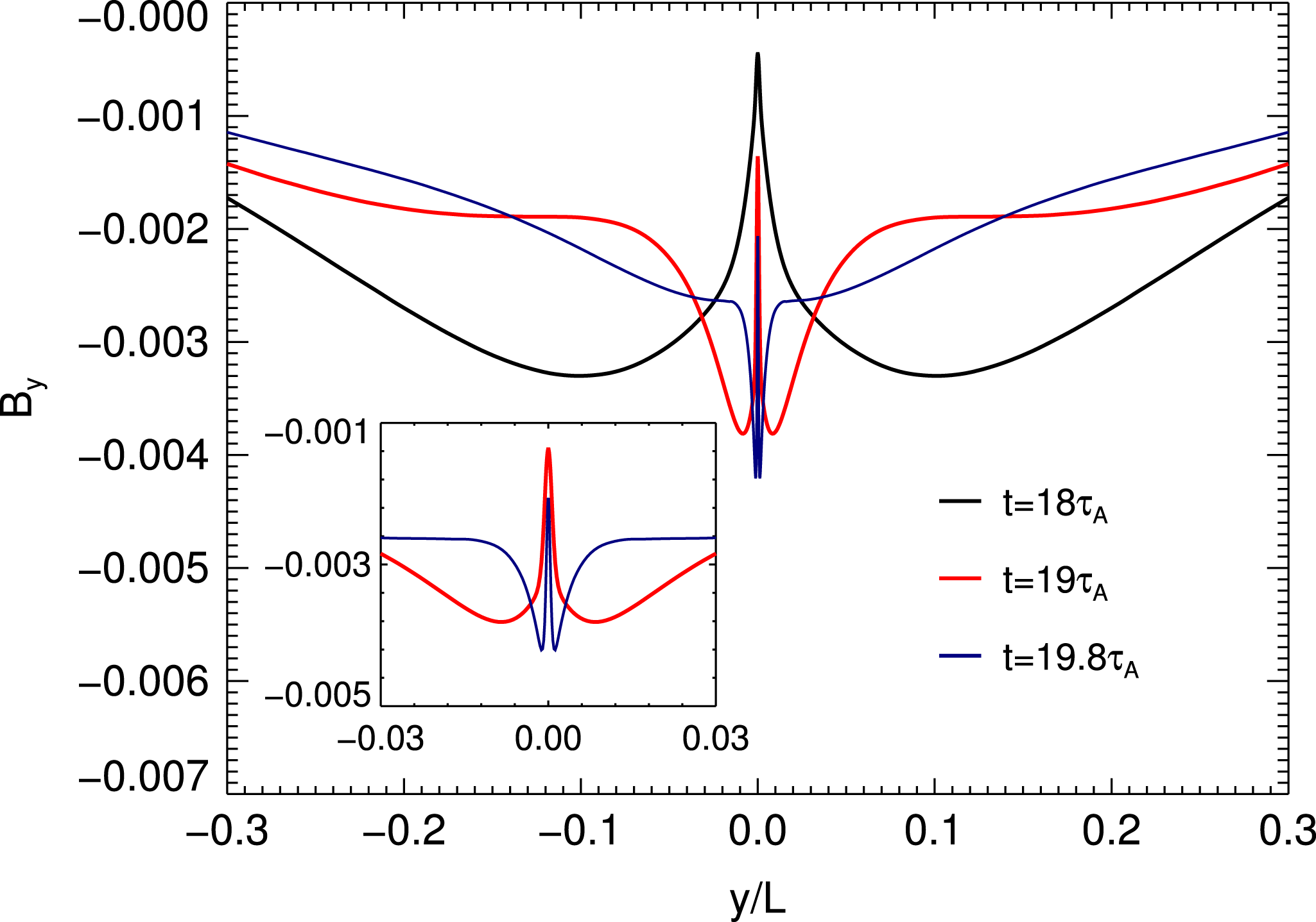
Figure 11. Hierarchy of tearing modes: plot of the magnetic field component along the inhomogeneous direction,
 $B_{y}$
, versus
$B_{y}$
, versus
 $y/L$
at position
$y/L$
at position
 $x/L=3.15$
of the current sheet shown in figure 9. Black colour corresponds to the primary tearing, the red one to
$x/L=3.15$
of the current sheet shown in figure 9. Black colour corresponds to the primary tearing, the red one to
 $n=1$
, and the blue to
$n=1$
, and the blue to
 $n=2$
. The inset is a blow up of the magnetic field for
$n=2$
. The inset is a blow up of the magnetic field for
 $n=1$
and
$n=1$
and
 $n=2$
(from Tenerani et al.
Reference Tenerani, Velli, Rappazzo and Pucci2015b
).
$n=2$
(from Tenerani et al.
Reference Tenerani, Velli, Rappazzo and Pucci2015b
).
Recent numerical two-dimensional simulations of ‘ideally’ unstable sheets at Lundquist numbers
 $S=10^{6}-10^{7}$
, have shown that the secondary current sheet lengthens exponentially at a rate close to the growth rate of the primary tearing (Tenerani et al.
Reference Tenerani, Velli, Rappazzo and Pucci2015b
). This is seen in figure 10, where different panels describing the time evolution of the secondary current sheet shown in figure 9 are displayed. The (half) thickness and length of such a sheet is now labelled
$S=10^{6}-10^{7}$
, have shown that the secondary current sheet lengthens exponentially at a rate close to the growth rate of the primary tearing (Tenerani et al.
Reference Tenerani, Velli, Rappazzo and Pucci2015b
). This is seen in figure 10, where different panels describing the time evolution of the secondary current sheet shown in figure 9 are displayed. The (half) thickness and length of such a sheet is now labelled
 $a_{1}$
and
$a_{1}$
and
 $L_{1}$
: (a) shows the profile of the out-of-plane current density
$L_{1}$
: (a) shows the profile of the out-of-plane current density
 $j_{z}(x,y)$
intensity along the current sheet at the neutral line
$j_{z}(x,y)$
intensity along the current sheet at the neutral line
 $y/L=0$
at different times, ranging from the end of the linear stage of the primary tearing up to the fully developed secondary instability. The latter can be recognized as the growth of a more intense current maximum in the middle of
$y/L=0$
at different times, ranging from the end of the linear stage of the primary tearing up to the fully developed secondary instability. The latter can be recognized as the growth of a more intense current maximum in the middle of
 $L_{1}$
, surrounded by two local minima, corresponding to two plasmoids, at about
$L_{1}$
, surrounded by two local minima, corresponding to two plasmoids, at about
 $t=19.2\unicode[STIX]{x1D70F}_{A}$
(green colour); in (b) we plot a cut of
$t=19.2\unicode[STIX]{x1D70F}_{A}$
(green colour); in (b) we plot a cut of
 $j_{z}(x,y)$
across the sheet at
$j_{z}(x,y)$
across the sheet at
 $x/L=3.15$
, at the same times. Such a secondary current sheet arises from the inner diffusion layer of the primary tearing: its thickness has indeed an almost constant value
$x/L=3.15$
, at the same times. Such a secondary current sheet arises from the inner diffusion layer of the primary tearing: its thickness has indeed an almost constant value
 $a_{1}/L\simeq 0.0015$
, that consistently scales with the macroscopic quantities as
$a_{1}/L\simeq 0.0015$
, that consistently scales with the macroscopic quantities as
 $a_{1}/L\simeq \unicode[STIX]{x1D6FF}_{i}/L\sim S^{-1/2}$
(see (3.2)). This can be seen from figure 10(b), for all times before the appearance of fully developed plasmoids (i.e.
$a_{1}/L\simeq \unicode[STIX]{x1D6FF}_{i}/L\sim S^{-1/2}$
(see (3.2)). This can be seen from figure 10(b), for all times before the appearance of fully developed plasmoids (i.e.
 $t=19.2\unicode[STIX]{x1D70F}_{A}$
as mentioned above); in (c) we plot the time evolution of
$t=19.2\unicode[STIX]{x1D70F}_{A}$
as mentioned above); in (c) we plot the time evolution of
 $L_{1}$
(green dots),
$L_{1}$
(green dots),
 $a_{1}/L_{1}$
(blue dots) and the threshold conditions for instability corresponding to the ‘ideal’ tearing (red dotted line), to the viscous SP (light blue dotted line), and to the flow-modified ‘ideal’ tearing discussed in § 3.1 (black dashed and dot-dashed lines). As can be seen, this current sheet breaks up during the collapse once it becomes unstable on the local Alfvén time, hence before the SP aspect ratio is reached and in good agreement with the flow-modified ‘ideal’ tearing (Landi et al.
Reference Landi, Del Zanna, Papini, Pucci and Velli2015; Tenerani et al.
Reference Tenerani, Velli, Rappazzo and Pucci2015b
), finally giving rise to another thinner sheet (see the green curves in figure 10(a,b). In figure 11 we show the profile of the magnetic field
$a_{1}/L_{1}$
(blue dots) and the threshold conditions for instability corresponding to the ‘ideal’ tearing (red dotted line), to the viscous SP (light blue dotted line), and to the flow-modified ‘ideal’ tearing discussed in § 3.1 (black dashed and dot-dashed lines). As can be seen, this current sheet breaks up during the collapse once it becomes unstable on the local Alfvén time, hence before the SP aspect ratio is reached and in good agreement with the flow-modified ‘ideal’ tearing (Landi et al.
Reference Landi, Del Zanna, Papini, Pucci and Velli2015; Tenerani et al.
Reference Tenerani, Velli, Rappazzo and Pucci2015b
), finally giving rise to another thinner sheet (see the green curves in figure 10(a,b). In figure 11 we show the profile of the magnetic field
 $B_{y}(y,x)$
,
$B_{y}(y,x)$
,
 $x/L=3.15$
, across the centre of the same sheet shown in figure 9, at three different times. The magnetic field profile displays a striking if unsurprising similarity to the tearing eigenfunctions (compare also with figure 3
a), as well as a hierarchical structure: the black colour corresponds to the magnetic perturbation grown during the primary instability; the red and blue colours correspond to the first and to the second secondary instability, magnified in the inset. In particular, note that the red profile as seen in the inset is the same as the black profile of the main figure. What this means is that each magnetic field perturbation that will lead to a new sheet grows within the inner diffusion layer of the unstable mode developed within the previous sheet. This in turn suggests that formation of ever smaller scales occurs via a recursive process of X-point formation, collapse and break up, reminiscent of the so-called ‘fractal’ reconnection scenario originally proposed by Shibata & Tanuma (Reference Shibata and Tanuma2001), that can be accounted for by the ‘ideal’ tearing instability.
$x/L=3.15$
, across the centre of the same sheet shown in figure 9, at three different times. The magnetic field profile displays a striking if unsurprising similarity to the tearing eigenfunctions (compare also with figure 3
a), as well as a hierarchical structure: the black colour corresponds to the magnetic perturbation grown during the primary instability; the red and blue colours correspond to the first and to the second secondary instability, magnified in the inset. In particular, note that the red profile as seen in the inset is the same as the black profile of the main figure. What this means is that each magnetic field perturbation that will lead to a new sheet grows within the inner diffusion layer of the unstable mode developed within the previous sheet. This in turn suggests that formation of ever smaller scales occurs via a recursive process of X-point formation, collapse and break up, reminiscent of the so-called ‘fractal’ reconnection scenario originally proposed by Shibata & Tanuma (Reference Shibata and Tanuma2001), that can be accounted for by the ‘ideal’ tearing instability.
Recursive models have been introduced for describing the different stages of such sublayer formation (sometimes also referred to as the multiple X-point reconnection stage) and how many plasmoids are generated during the fully nonlinear evolution (Daughton et al.
Reference Daughton, Roytershteyn, Albright, Karimabadi, Yin and Bowers2009; Huang & Bhattacharjee Reference Huang and Bhattacharjee2010; Uzdensky et al.
Reference Uzdensky, Loureiro and Schekochihin2010; Ji & Daughton Reference Ji and Daghton2011). To this end, it is convenient now to label with an
 $n$
the (half) length
$n$
the (half) length
 $L_{n}$
, thickness
$L_{n}$
, thickness
 $a_{n}$
, and the local Lundquist number
$a_{n}$
, and the local Lundquist number
 $S_{n}=(L_{n}/L)\,S$
of the
$S_{n}=(L_{n}/L)\,S$
of the
 $n$
th current sheet. Previous models assume that at each step current sheets become unstable giving rise to smaller ones with length
$n$
th current sheet. Previous models assume that at each step current sheets become unstable giving rise to smaller ones with length
 $L_{n}=L_{n-1}/N_{n-1}$
, where
$L_{n}=L_{n-1}/N_{n-1}$
, where
 $N_{n}$
is the number of plasmoids at step
$N_{n}$
is the number of plasmoids at step
 $n$
and thickness defined by the SP scaling, therefore
$n$
and thickness defined by the SP scaling, therefore
 $a_{n}=L_{n}S_{n}^{-1/2}$
. In particular, Ji & Daughton (Reference Ji and Daghton2011) used a phenomenological scaling for the number of plasmoids
$a_{n}=L_{n}S_{n}^{-1/2}$
. In particular, Ji & Daughton (Reference Ji and Daghton2011) used a phenomenological scaling for the number of plasmoids
 $N_{n}=(S_{n}/S_{c})^{\unicode[STIX]{x1D6FD}}$
, where
$N_{n}=(S_{n}/S_{c})^{\unicode[STIX]{x1D6FD}}$
, where
 $\unicode[STIX]{x1D6FD}$
is left as a free parameter, and
$\unicode[STIX]{x1D6FD}$
is left as a free parameter, and
 $S_{c}\simeq 10^{4}$
is the empirical critical Lundquist number for onset of plasmoid instability; such a scaling describing the number of plasmoids has been commonly adopted by other authors as well, motivated by the linear theory – although, strictly speaking, the linear theory as developed does not predict a renormalization to
$S_{c}\simeq 10^{4}$
is the empirical critical Lundquist number for onset of plasmoid instability; such a scaling describing the number of plasmoids has been commonly adopted by other authors as well, motivated by the linear theory – although, strictly speaking, the linear theory as developed does not predict a renormalization to
 $S_{c}$
, and therefore it yields a far larger value for
$S_{c}$
, and therefore it yields a far larger value for
 $N_{n}$
. Those assumptions lead to an infinite hierarchy, where secondary current sheets never cross the presumed stability threshold
$N_{n}$
. Those assumptions lead to an infinite hierarchy, where secondary current sheets never cross the presumed stability threshold
 $S_{n}\lesssim S_{c}$
, and for this reason Ji & Daughton (Reference Ji and Daghton2011) impose a minimum number of plasmoids
$S_{n}\lesssim S_{c}$
, and for this reason Ji & Daughton (Reference Ji and Daghton2011) impose a minimum number of plasmoids
 $N_{min}$
as a cutoff to find the maximum index of the hierarchy,
$N_{min}$
as a cutoff to find the maximum index of the hierarchy,
 $n_{\ast }$
. Assuming also that each current sheet becomes unstable, they find that the total, final number
$n_{\ast }$
. Assuming also that each current sheet becomes unstable, they find that the total, final number
 ${\mathcal{N}}$
of plasmoids is
${\mathcal{N}}$
of plasmoids is
 ${\mathcal{N}}\simeq (S/S_{c})^{z}$
, with
${\mathcal{N}}\simeq (S/S_{c})^{z}$
, with
 $z\sim 0.76,\,0.96$
for
$z\sim 0.76,\,0.96$
for
 $n_{\ast }\simeq 3,\,2$
and
$n_{\ast }\simeq 3,\,2$
and
 $\unicode[STIX]{x1D6FD}=3/8,\,0.8$
. This heuristic argument then leads to values for the number of plasmoids consistent with that found directly in numerical simulations (Cassak, Shay & Drake Reference Cassak, Shay and Drake2009; Daughton et al.
Reference Daughton, Roytershteyn, Albright, Karimabadi, Yin and Bowers2009; Huang & Bhattacharjee Reference Huang and Bhattacharjee2010).
$\unicode[STIX]{x1D6FD}=3/8,\,0.8$
. This heuristic argument then leads to values for the number of plasmoids consistent with that found directly in numerical simulations (Cassak, Shay & Drake Reference Cassak, Shay and Drake2009; Daughton et al.
Reference Daughton, Roytershteyn, Albright, Karimabadi, Yin and Bowers2009; Huang & Bhattacharjee Reference Huang and Bhattacharjee2010).
Before illustrating our recursive model, it is worth commenting on the question of the scaling of the number of islands with the Lundquist number as the plasmoid instability develops. Numerical simulations appear to have shown a number compatible with the scaling of the plasmoid instability on Sweet–Parker sheets, although generally speaking simulations tend to have Lundquist numbers which, already at the macroscopic scale, are quite close to the critical one for stability threshold (
 $S_{c}$
) (Bhattacharjee et al.
Reference Battacharjee, Huang, Yang and Rogers2009; Huang & Bhattacharjee Reference Huang and Bhattacharjee2010). In this sense it is surprising that a scaling relationship such as
$S_{c}$
) (Bhattacharjee et al.
Reference Battacharjee, Huang, Yang and Rogers2009; Huang & Bhattacharjee Reference Huang and Bhattacharjee2010). In this sense it is surprising that a scaling relationship such as
 $N_{SP}\sim S^{3/8}$
, derived under the assumptions that flows may be completely neglected, might hold true. The same might be said of the scaling of islands along the sheet once nonlinearities become important, where results closer to
$N_{SP}\sim S^{3/8}$
, derived under the assumptions that flows may be completely neglected, might hold true. The same might be said of the scaling of islands along the sheet once nonlinearities become important, where results closer to
 ${\mathcal{N}}\sim S$
are found (Huang & Bhattacharjee Reference Huang and Bhattacharjee2010). The reason is that counting X-points is equivalent to precisely determining the topology of the magnetic field at very small scales, while the (maximum possible) value of the Lundquist number
${\mathcal{N}}\sim S$
are found (Huang & Bhattacharjee Reference Huang and Bhattacharjee2010). The reason is that counting X-points is equivalent to precisely determining the topology of the magnetic field at very small scales, while the (maximum possible) value of the Lundquist number
 $S$
is essentially determined by the number of grid points. A scaling
$S$
is essentially determined by the number of grid points. A scaling
 ${\mathcal{N}}\sim S$
along an extended one-dimensional sheet implies that the number of islands grows linearly with resolution. In such a reconnection configuration, the line is the original central current sheet neutral line: when moving to more general two-dimensional configurations, very high resolution simulations of fully developed turbulence show a number of X-points appearing to scale as
${\mathcal{N}}\sim S$
along an extended one-dimensional sheet implies that the number of islands grows linearly with resolution. In such a reconnection configuration, the line is the original central current sheet neutral line: when moving to more general two-dimensional configurations, very high resolution simulations of fully developed turbulence show a number of X-points appearing to scale as
 ${\mathcal{N}}\sim S^{3/2}$
(Wan et al.
Reference Wan, Mettheaus, Servidio and Oughton2013). Following our previous statement, the corresponding upper limit set by resolution on the scaling of the number of island would be
${\mathcal{N}}\sim S^{3/2}$
(Wan et al.
Reference Wan, Mettheaus, Servidio and Oughton2013). Following our previous statement, the corresponding upper limit set by resolution on the scaling of the number of island would be
 ${\mathcal{N}}\sim S^{2}$
, so it appears that the scaling found by Wan et al. (Reference Wan, Mettheaus, Servidio and Oughton2013) is reasonable. In other words, as stated by Wan et al. (Reference Wan, Mettheaus, Servidio and Oughton2013) ‘[
${\mathcal{N}}\sim S^{2}$
, so it appears that the scaling found by Wan et al. (Reference Wan, Mettheaus, Servidio and Oughton2013) is reasonable. In other words, as stated by Wan et al. (Reference Wan, Mettheaus, Servidio and Oughton2013) ‘[
 $\ldots$
] lack of adequate numerical resolution can easily increase the number of detected X-points, thus producing non-physical results. Generally speaking, one requires high spatial resolution, to at least three times the Kolmogorov dissipation wavenumber, when using the pseudo-spectral approach that we have employed.’
$\ldots$
] lack of adequate numerical resolution can easily increase the number of detected X-points, thus producing non-physical results. Generally speaking, one requires high spatial resolution, to at least three times the Kolmogorov dissipation wavenumber, when using the pseudo-spectral approach that we have employed.’
Here we reconsider the recursive reconnection model, but following more in detail the ‘ideal’ tearing scenario guided by our numerical results. We point out that a hierarchy of sublayers form anywhere in regions where currents have room to collapse. In this regard, boundary conditions may play a fundamental role, if the system size is not large enough to allow the dynamics to develop freely. Nevertheless, this limitation is automatically overcome in simulations of ideally unstable current sheets, since the wavelength of the ideal mode,
 $\unicode[STIX]{x1D706}_{i}\sim 2\unicode[STIX]{x03C0}\,S^{-1/6}$
, is much smaller than the length of the current sheet (approximately given by the size of the simulation domain). Of course, the collapse of X-points cannot and does not occur uniformly along the sheet, rather, nonlinear evolution is determined by the competition and interplay between multiple recursive X-point formation within the most intense currents, and an inverse cascade of merging plasmoids, as can also be seen by inspection of figure 7. Therefore, differently from the models discussed above, we apply the recursive idea to a given secondary current sheet, so that our model leaves the final number of plasmoids generated undefined. It instead provides a prediction of the total number of steps
$\unicode[STIX]{x1D706}_{i}\sim 2\unicode[STIX]{x03C0}\,S^{-1/6}$
, is much smaller than the length of the current sheet (approximately given by the size of the simulation domain). Of course, the collapse of X-points cannot and does not occur uniformly along the sheet, rather, nonlinear evolution is determined by the competition and interplay between multiple recursive X-point formation within the most intense currents, and an inverse cascade of merging plasmoids, as can also be seen by inspection of figure 7. Therefore, differently from the models discussed above, we apply the recursive idea to a given secondary current sheet, so that our model leaves the final number of plasmoids generated undefined. It instead provides a prediction of the total number of steps
 $n_{\ast }$
and of the time scale of the recursive process itself.
$n_{\ast }$
and of the time scale of the recursive process itself.
Since tearing is a multi-scale process, in the sense that it involves the formation of an inner singular layer, we also introduce the thickness of such inner layer
 $\unicode[STIX]{x1D6FF}_{n}$
of the
$\unicode[STIX]{x1D6FF}_{n}$
of the
 $n$
th unstable current sheet (for us
$n$
th unstable current sheet (for us
 $n\geqslant 1$
), and we define the local Alfvén time
$n\geqslant 1$
), and we define the local Alfvén time
 $\unicode[STIX]{x1D70F}_{A,n}=(L_{n}/L)\,\unicode[STIX]{x1D70F}_{A}$
. We rely on the following assumptions based on observations of our simulation results: first, that current sheets are lengthening and that they become unstable when the local critical aspect ratio is reached; second, we do not make any assumption on the length
$\unicode[STIX]{x1D70F}_{A,n}=(L_{n}/L)\,\unicode[STIX]{x1D70F}_{A}$
. We rely on the following assumptions based on observations of our simulation results: first, that current sheets are lengthening and that they become unstable when the local critical aspect ratio is reached; second, we do not make any assumption on the length
 $L_{n}$
, as is done in other recursive models (Shibata & Tanuma Reference Shibata and Tanuma2001; Ji & Daughton Reference Ji and Daghton2011), but, on the contrary, we observe that the thickness
$L_{n}$
, as is done in other recursive models (Shibata & Tanuma Reference Shibata and Tanuma2001; Ji & Daughton Reference Ji and Daghton2011), but, on the contrary, we observe that the thickness
 $a_{n}$
corresponds to the inner diffusion layer of the
$a_{n}$
corresponds to the inner diffusion layer of the
 $(n-1)$
th tearing,
$(n-1)$
th tearing,
 $\unicode[STIX]{x1D6FF}_{n-1}$
. These two requirements translate respectively into
$\unicode[STIX]{x1D6FF}_{n-1}$
. These two requirements translate respectively into
 $$\begin{eqnarray}\frac{a_{n}}{L_{n}}\sim S_{n}^{-1/3},\quad \frac{a_{n}}{L_{n-1}}\sim S_{n-1}^{-1/2},\end{eqnarray}$$
where for simplicity we have neglected the stabilizing effect of viscosity and of plasma flows, but which should be retained for the lower values of
 $S_{n}$
(see § 3.1). Expressions given in (5.1) yield the following scaling laws:
$S_{n}$
(see § 3.1). Expressions given in (5.1) yield the following scaling laws:
 $$\begin{eqnarray}L_{n}=L\,S^{-1+(3/4)^{n}},\quad \unicode[STIX]{x1D70F}_{A,n}=\frac{L_{n}}{L}\,\unicode[STIX]{x1D70F}_{A},\quad S_{n}=S^{(3/4)^{n}}.\end{eqnarray}$$
Considering typical coronal conditions, for which
 $L\simeq 10^{9}$
cm,
$L\simeq 10^{9}$
cm,
 $B_{0}\simeq 50$
G, the number density
$B_{0}\simeq 50$
G, the number density
 $n_{0}\simeq 10^{9}~\text{cm}^{-3}$
and the temperature
$n_{0}\simeq 10^{9}~\text{cm}^{-3}$
and the temperature
 $T\simeq 10^{6}$
K, then the macroscopic Lundquist number is
$T\simeq 10^{6}$
K, then the macroscopic Lundquist number is
 $S\simeq 10^{13}$
(Braginkii Reference Braginskii1965). The sequences of
$S\simeq 10^{13}$
(Braginkii Reference Braginskii1965). The sequences of
 $L_{n}$
and of
$L_{n}$
and of
 $S_{n}$
for
$S_{n}$
for
 $S=10^{13}$
are represented in figure 12, showing that the formation of microscopic scales occurs very rapidly. In this case, after a number of steps
$S=10^{13}$
are represented in figure 12, showing that the formation of microscopic scales occurs very rapidly. In this case, after a number of steps
 $n_{\ast }\simeq 4$
the local Lundquist number reaches
$n_{\ast }\simeq 4$
the local Lundquist number reaches
 $S_{n_{\ast }}\simeq 10^{4}$
, the region close to where one expects to find complete flow-driven stabilization. The time required to reach this marginally stable state gives an indication of the time scale for the complete disruption of the original current sheet, and is given by the time required to trigger the first instability
$S_{n_{\ast }}\simeq 10^{4}$
, the region close to where one expects to find complete flow-driven stabilization. The time required to reach this marginally stable state gives an indication of the time scale for the complete disruption of the original current sheet, and is given by the time required to trigger the first instability
 $\unicode[STIX]{x1D70F}_{0}$
(
$\unicode[STIX]{x1D70F}_{0}$
(
 $\unicode[STIX]{x1D70F}_{0}\simeq \unicode[STIX]{x1D70F}_{i}$
) plus the time of the recursive reconnection, that for
$\unicode[STIX]{x1D70F}_{0}\simeq \unicode[STIX]{x1D70F}_{i}$
) plus the time of the recursive reconnection, that for
 $S=10^{13}$
is about
$S=10^{13}$
is about
 $$\begin{eqnarray}\unicode[STIX]{x1D70F}\simeq \unicode[STIX]{x1D70F}_{0}+\mathop{\sum }_{n=1}^{n_{\ast }}\unicode[STIX]{x1D70F}_{A,n}\simeq (10-100)\unicode[STIX]{x1D70F}_{A}+5\times 10^{-4}\unicode[STIX]{x1D70F}_{A}.\end{eqnarray}$$
Formation of smaller scales can mediate the transition to a Hall (or kinetic) reconnection regime, when the ion scales are reached dynamically (Cassak et al.
Reference Cassak, Shay and Drake2005; Daughton et al.
Reference Daughton, Roytershteyn, Albright, Karimabadi, Yin and Bowers2009; Shepherd & Cassak Reference Shepherd and Cassak2010; Huang et al.
Reference Huang, Bhattacharjee and Sullivan2011). If ion scales are formed during the recursive reconnection, e.g.
 $a_{n}\simeq d_{i}$
, then different scalings should be adopted from that moment on. For instance, with the parameters chosen above as representative of the solar corona, the normalized ion inertial length turns out to be about
$a_{n}\simeq d_{i}$
, then different scalings should be adopted from that moment on. For instance, with the parameters chosen above as representative of the solar corona, the normalized ion inertial length turns out to be about
 $d_{i}/L\simeq 10^{-7}$
, which is of the same order of the thickness formed at the first step,
$d_{i}/L\simeq 10^{-7}$
, which is of the same order of the thickness formed at the first step,
 $a_{1}/L$
, for
$a_{1}/L$
, for
 $S=10^{13}$
. A study including the Hall effect is however necessary to assess with more precision at which thickness the MHD scalings used so far are modified. The main point here is that regardless of whether MHD or a specific kinetic regime is the more suitable model, ‘ideal’ tearing provides a clear well-defined threshold for the onset of fast reconnection (Del Sarto et al.
Reference Del Sarto, Pucci, Tenerani and Velli2016), so that (5.2) can be extended to kinetic regimes as well.
$S=10^{13}$
. A study including the Hall effect is however necessary to assess with more precision at which thickness the MHD scalings used so far are modified. The main point here is that regardless of whether MHD or a specific kinetic regime is the more suitable model, ‘ideal’ tearing provides a clear well-defined threshold for the onset of fast reconnection (Del Sarto et al.
Reference Del Sarto, Pucci, Tenerani and Velli2016), so that (5.2) can be extended to kinetic regimes as well.

Figure 12. Plot of the sequence
 $L_{n}/L$
(a) and
$L_{n}/L$
(a) and
 $S_{n}$
(b) for
$S_{n}$
(b) for
 $S=10^{13}$
, see (5.2).
$S=10^{13}$
, see (5.2).
6 Comparison with previous models
In spite of the different initial conditions, the evolution of the current sheet formed during the nonlinear stage of the ‘ideal’ tearing, as shown for instance in figure 9, is qualitatively reminiscent of, and can be compared to the ‘embedded reconnection’ scenario (Shay et al.
Reference Shay, Drake, Swisdak and Rogers2004; Cassak & Drake Reference Cassak and Drake2009), in which the diffusion layer is embedded within a thicker underlying current sheet. The argument of the embedded layer led Cassak & Drake (Reference Cassak and Drake2009) to take into account the increasing Alfvén speed due to pile up just upstream the inner diffusion layer, and to find in this way the scaling
 $a_{1}/L_{1}\sim S_{1}^{-1/3}$
for onset of instability (in order to avoid confusion, we adopt here our notation, and
$a_{1}/L_{1}\sim S_{1}^{-1/3}$
for onset of instability (in order to avoid confusion, we adopt here our notation, and
 $S_{1}=v_{A}L_{1}/\unicode[STIX]{x1D702}$
). Nevertheless, their scaling has a different origin and it stems from the criterion to destabilize a SP sheet, when the local Lundquist number exceeds the value
$S_{1}=v_{A}L_{1}/\unicode[STIX]{x1D702}$
). Nevertheless, their scaling has a different origin and it stems from the criterion to destabilize a SP sheet, when the local Lundquist number exceeds the value
 $S_{c}=10^{4}$
. Cassak & Drake (Reference Cassak and Drake2009) assumed that the diffusion layer ultimately becomes an unstable SP sheet, which however satisfies
$S_{c}=10^{4}$
. Cassak & Drake (Reference Cassak and Drake2009) assumed that the diffusion layer ultimately becomes an unstable SP sheet, which however satisfies
 $a_{1}/L_{1}\sim S_{up}^{-1/2}$
,
$a_{1}/L_{1}\sim S_{up}^{-1/2}$
,
 $S_{up}$
being the upstream Lundquist number, defined through the upstream magnetic field
$S_{up}$
being the upstream Lundquist number, defined through the upstream magnetic field
 $B_{up}$
and
$B_{up}$
and
 $L_{1}$
;
$L_{1}$
;
 $B_{up}$
can be approximated near the neutral line by linearizing the magnetic field, hence
$B_{up}$
can be approximated near the neutral line by linearizing the magnetic field, hence
 $B_{up}\simeq B_{0}(a_{1}/a)$
. Direct substitution of
$B_{up}\simeq B_{0}(a_{1}/a)$
. Direct substitution of
 $B_{up}$
into the SP scaling for the inverse aspect ratio yields the same exponent
$B_{up}$
into the SP scaling for the inverse aspect ratio yields the same exponent
 $\unicode[STIX]{x1D6FC}=1/3$
for onset of instability. On the other hand, the ‘ideal’ tearing scaling derives from requiring an
$\unicode[STIX]{x1D6FC}=1/3$
for onset of instability. On the other hand, the ‘ideal’ tearing scaling derives from requiring an
 $S$
-independent growth rate from the complete eigenmode analysis of tearing instability, and the presence of flows modifies the scaling exponent
$S$
-independent growth rate from the complete eigenmode analysis of tearing instability, and the presence of flows modifies the scaling exponent
 $\unicode[STIX]{x1D6FC}$
according to (3.3). For their values
$\unicode[STIX]{x1D6FC}$
according to (3.3). For their values
 $S_{1}\simeq 2.5\times 10^{4}-10^{5}$
the exponent
$S_{1}\simeq 2.5\times 10^{4}-10^{5}$
the exponent
 $\unicode[STIX]{x1D6FC}_{c}\simeq 0.48-0.46$
, that give an unstable current sheet when
$\unicode[STIX]{x1D6FC}_{c}\simeq 0.48-0.46$
, that give an unstable current sheet when
 $a_{1}/L_{1}\sim S_{1}^{-\unicode[STIX]{x1D6FC}_{c}}\simeq 0.007-0.005$
. These estimates are in agreement with the unstable inverse aspect ratios found in the Cassak & Drake (Reference Cassak and Drake2009) paper.
$a_{1}/L_{1}\sim S_{1}^{-\unicode[STIX]{x1D6FC}_{c}}\simeq 0.007-0.005$
. These estimates are in agreement with the unstable inverse aspect ratios found in the Cassak & Drake (Reference Cassak and Drake2009) paper.
It is interesting to note that the scaling exponent
 $\unicode[STIX]{x1D6FC}=1/3$
as an instability criterion was also derived by Shibata & Tanuma (Reference Shibata and Tanuma2001) in the framework of ‘fractal’ reconnection, introduced for the first time by those authors as a possible phenomenological model for current sheet disruption during solar flares. Based on the argument of Biskamp (Reference Biskamp1986), Shibata & Tanuma (Reference Shibata and Tanuma2001) searched for a condition to overcome the stabilizing effect of flows on the tearing instability. They concluded that, given a current sheet of inverse aspect ratio
$\unicode[STIX]{x1D6FC}=1/3$
as an instability criterion was also derived by Shibata & Tanuma (Reference Shibata and Tanuma2001) in the framework of ‘fractal’ reconnection, introduced for the first time by those authors as a possible phenomenological model for current sheet disruption during solar flares. Based on the argument of Biskamp (Reference Biskamp1986), Shibata & Tanuma (Reference Shibata and Tanuma2001) searched for a condition to overcome the stabilizing effect of flows on the tearing instability. They concluded that, given a current sheet of inverse aspect ratio
 $a_{n}/L_{n}$
, the maximum growth rate of the tearing had to exceed the plasmoid evacuation rate
$a_{n}/L_{n}$
, the maximum growth rate of the tearing had to exceed the plasmoid evacuation rate
 $\unicode[STIX]{x1D6E4}_{n}\simeq v_{A}/L_{n}=1/\unicode[STIX]{x1D70F}_{A,n}$
for the tearing to develop (in the end, effects of flows on the growth rate are not taken into account in their model). Shibata & Tanuma (Reference Shibata and Tanuma2001) can find in this way that the current sheet must at least have an inverse aspect ratio
$\unicode[STIX]{x1D6E4}_{n}\simeq v_{A}/L_{n}=1/\unicode[STIX]{x1D70F}_{A,n}$
for the tearing to develop (in the end, effects of flows on the growth rate are not taken into account in their model). Shibata & Tanuma (Reference Shibata and Tanuma2001) can find in this way that the current sheet must at least have an inverse aspect ratio
 $a_{n}/L_{n}\leqslant S_{n}^{-1/3}$
in order to become unstable. Again, the result of Shibata & Tanuma (Reference Shibata and Tanuma2001) stems from a different line of thought, as they searched for a maximum growth rate larger than the inverse of the ideal time
$a_{n}/L_{n}\leqslant S_{n}^{-1/3}$
in order to become unstable. Again, the result of Shibata & Tanuma (Reference Shibata and Tanuma2001) stems from a different line of thought, as they searched for a maximum growth rate larger than the inverse of the ideal time
 $\unicode[STIX]{x1D70F}_{A,n}$
, and not for an ‘ideal’ growth rate, independent from the Lundquist number. Next, in their ‘fractal’ model the authors assume that the length for each sublayer corresponds to the wavelength of the fastest growing mode, i.e.
$\unicode[STIX]{x1D70F}_{A,n}$
, and not for an ‘ideal’ growth rate, independent from the Lundquist number. Next, in their ‘fractal’ model the authors assume that the length for each sublayer corresponds to the wavelength of the fastest growing mode, i.e.
 $L_{n}=2\unicode[STIX]{x03C0}/k_{n}$
, that yields a different scaling law for
$L_{n}=2\unicode[STIX]{x03C0}/k_{n}$
, that yields a different scaling law for
 $L_{n}$
with respect to ours, having a weaker dependence on
$L_{n}$
with respect to ours, having a weaker dependence on
 $n$
.
$n$
.
7 Summary and discussion
We have given an overview of linear tearing instabilities within thin current sheets at arbitrary aspect ratios in resistive MHD and discussed some extensions, namely, Reduced MHD with inclusion of kinetic effects. Theory shows that fast reconnection, developing on time scales independent of the non-ideal terms in Ohm’s law, sets in at a critical aspect ratio
 $L/a_{i}$
that satisfies specific scaling laws with plasma parameters such as
$L/a_{i}$
that satisfies specific scaling laws with plasma parameters such as
 $S$
and
$S$
and
 $d_{e}/L$
. Such scaling laws can be modified by viscosity at large Prandtl numbers, or by kinetic effects when the inner diffusion layer is of the order of, or smaller than,
$d_{e}/L$
. Such scaling laws can be modified by viscosity at large Prandtl numbers, or by kinetic effects when the inner diffusion layer is of the order of, or smaller than,
 $\unicode[STIX]{x1D70C}_{s}$
and
$\unicode[STIX]{x1D70C}_{s}$
and
 $\unicode[STIX]{x1D70C}_{i}$
(Pucci & Velli Reference Pucci and Velli2014; Tenerani et al.
Reference Tenerani, Rappazzo, Velli and Pucci2015a
; Del Sarto et al.
Reference Del Sarto, Pucci, Tenerani and Velli2016). The main result that emerges from these studies is that in the asymptotic limit
$\unicode[STIX]{x1D70C}_{i}$
(Pucci & Velli Reference Pucci and Velli2014; Tenerani et al.
Reference Tenerani, Rappazzo, Velli and Pucci2015a
; Del Sarto et al.
Reference Del Sarto, Pucci, Tenerani and Velli2016). The main result that emerges from these studies is that in the asymptotic limit
 $S\rightarrow \infty$
or
$S\rightarrow \infty$
or
 $d_{e}/L\rightarrow 0$
a violent transition from a stable state (reconnecting over infinitely long times) to an ideally unstable one has to occur when approaching the critical thickness
$d_{e}/L\rightarrow 0$
a violent transition from a stable state (reconnecting over infinitely long times) to an ideally unstable one has to occur when approaching the critical thickness
 $a_{i}/L$
from above. The onset of fast reconnection cannot take place within current sheets that are thicker than critical, for sufficiently large values of
$a_{i}/L$
from above. The onset of fast reconnection cannot take place within current sheets that are thicker than critical, for sufficiently large values of
 $S$
: unstable modes at smaller aspect ratios,
$S$
: unstable modes at smaller aspect ratios,
 $L/a<L/a_{i}$
, have growth rates whose values tend to zero in the asymptotic limit, whereas, precisely at
$L/a<L/a_{i}$
, have growth rates whose values tend to zero in the asymptotic limit, whereas, precisely at
 $L/a_{i}$
, the full dispersion relation
$L/a_{i}$
, the full dispersion relation
 $\unicode[STIX]{x1D6FE}(k)$
becomes rapidly peaked around
$\unicode[STIX]{x1D6FE}(k)$
becomes rapidly peaked around
 $k_{m}$
(cf. for instance, figure 5
b), the ‘ideal’ mode being the only surviving one in the asymptotic limit; ‘ideal’ tearing onset, by breaking up the current on an ideal time scale, prevents the spontaneous formation of much larger aspect ratio current sheets, such as the Sweet–Parker one. Fully nonlinear MHD simulations show that the inner diffusion layer of the ideally reconnecting current sheet evolves during the nonlinear stage into an elongated secondary current sheet, that in turn becomes unstable to ‘ideal’ tearing at the local Alfvén time. This process of current sheet formation from of the inner diffusion layer proceeds in a recursive way at smaller and smaller scales, that can be accounted for by properly rescaling ‘ideal’ tearing to the local length of the sheet (Landi et al.
Reference Landi, Del Zanna, Papini, Pucci and Velli2015; Tenerani et al.
Reference Tenerani, Velli, Rappazzo and Pucci2015b
), even though an appropriate statistical study of the fully nonlinear stage has not been completed yet because of the incredibly high resolutions required to resolve the recursive formation of plasmoids down to the dissipative scales.
$k_{m}$
(cf. for instance, figure 5
b), the ‘ideal’ mode being the only surviving one in the asymptotic limit; ‘ideal’ tearing onset, by breaking up the current on an ideal time scale, prevents the spontaneous formation of much larger aspect ratio current sheets, such as the Sweet–Parker one. Fully nonlinear MHD simulations show that the inner diffusion layer of the ideally reconnecting current sheet evolves during the nonlinear stage into an elongated secondary current sheet, that in turn becomes unstable to ‘ideal’ tearing at the local Alfvén time. This process of current sheet formation from of the inner diffusion layer proceeds in a recursive way at smaller and smaller scales, that can be accounted for by properly rescaling ‘ideal’ tearing to the local length of the sheet (Landi et al.
Reference Landi, Del Zanna, Papini, Pucci and Velli2015; Tenerani et al.
Reference Tenerani, Velli, Rappazzo and Pucci2015b
), even though an appropriate statistical study of the fully nonlinear stage has not been completed yet because of the incredibly high resolutions required to resolve the recursive formation of plasmoids down to the dissipative scales.
In the solar corona, where inter-species collisions usually provide the dominant dissipation mechanism for reconnection, the Lundquist numbers are
 $S\simeq 10^{12}-10^{14}$
. For instance, for
$S\simeq 10^{12}-10^{14}$
. For instance, for
 $S=10^{13}$
the critical inverse aspect ratio is
$S=10^{13}$
the critical inverse aspect ratio is
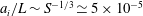 $a_{i}/L\sim S^{-1/3}\simeq 5\times 10^{-5}$
, i.e. for a loop structure of length
$a_{i}/L\sim S^{-1/3}\simeq 5\times 10^{-5}$
, i.e. for a loop structure of length
 $L\simeq 10^{9}$
cm the critical thickness would be
$L\simeq 10^{9}$
cm the critical thickness would be
 $a_{i}\simeq 500$
m, with an inner layer of about
$a_{i}\simeq 500$
m, with an inner layer of about
 $\unicode[STIX]{x1D6FF}_{i}\simeq 3$
m, intermediate between the ion inertial length,
$\unicode[STIX]{x1D6FF}_{i}\simeq 3$
m, intermediate between the ion inertial length,
 $d_{i}\simeq 10$
m, and the ion Larmor radius,
$d_{i}\simeq 10$
m, and the ion Larmor radius,
 $\unicode[STIX]{x1D70C}_{i}\simeq 10$
cm. Two-fluid effects related to the Hall term in the generalized Ohm’s law need therefore to be investigated to give a more realistic description of ideally unstable current sheets. Inclusion of such effects becomes however necessary when nonlinearities naturally lead to the formation of microscopic scales, e.g. during recursive reconnection.
$\unicode[STIX]{x1D70C}_{i}\simeq 10$
cm. Two-fluid effects related to the Hall term in the generalized Ohm’s law need therefore to be investigated to give a more realistic description of ideally unstable current sheets. Inclusion of such effects becomes however necessary when nonlinearities naturally lead to the formation of microscopic scales, e.g. during recursive reconnection.
A different regime describes the Earth’s magnetosphere, and in particular the magnetotail, for which a kinetic description is more suitable (Coppi, Laval & Pellat Reference Coppi, Laval and Pellat1966; Schindler Reference Schindler1974; Vasyliunas Reference Vasyliunas1975; Daughton Reference Daughton1999; Sitnov et al.
Reference Sitnov, Merkin, Swisdak, Motoba, Buzulukova, Moore, Mauk and Ohtani2014). Here, resistive reconnection, due either to inter-specie collisions or to wave–particle scattering (Coroniti Reference Coroniti1985), is usually dominated by reconnection induced by electron inertia. Assuming values of plasma density
 $n_{0}\simeq 0.1~\text{cm}^{-3}$
, electron temperature
$n_{0}\simeq 0.1~\text{cm}^{-3}$
, electron temperature
 $T_{e}\simeq 10^{7}$
K (for simplicity we consider ions and electrons at the same temperature) and magnetic field
$T_{e}\simeq 10^{7}$
K (for simplicity we consider ions and electrons at the same temperature) and magnetic field
 $B_{0}\simeq 10^{-4}$
G, and taking as typical sheet length
$B_{0}\simeq 10^{-4}$
G, and taking as typical sheet length
 $L\simeq 10^{9}$
cm, then the Lundquist number ranges from
$L\simeq 10^{9}$
cm, then the Lundquist number ranges from
 $S\simeq 10^{10}$
(for wave–particle scattering; Eastwood et al. (Reference Eastwood, Phan, Bale and Tjulin2009)) to
$S\simeq 10^{10}$
(for wave–particle scattering; Eastwood et al. (Reference Eastwood, Phan, Bale and Tjulin2009)) to
 $S\simeq 10^{15}$
(for standard collisions), whereas
$S\simeq 10^{15}$
(for standard collisions), whereas
 $d_{e}^{2}/L^{2}\simeq 10^{-6}$
. The electron skin depth is about
$d_{e}^{2}/L^{2}\simeq 10^{-6}$
. The electron skin depth is about
 $d_{e}\simeq 10$
km and the ion length scales are
$d_{e}\simeq 10$
km and the ion length scales are
 $\unicode[STIX]{x1D70C}_{i}\simeq \unicode[STIX]{x1D70C}_{s}\simeq 300$
km, of the order of the ion skin depth,
$\unicode[STIX]{x1D70C}_{i}\simeq \unicode[STIX]{x1D70C}_{s}\simeq 300$
km, of the order of the ion skin depth,
 $d_{i}\simeq 700$
km. Ionic scales are not far from the thickness of the central current sheet, that is observed to thin down to about 1000 km during the substorm growth phase, and for these parameters the kinetic equation (3.9) predicts
$d_{i}\simeq 700$
km. Ionic scales are not far from the thickness of the central current sheet, that is observed to thin down to about 1000 km during the substorm growth phase, and for these parameters the kinetic equation (3.9) predicts
 $a_{i}\simeq 400$
km. However, what is the effective driving mechanism for collisionless reconnection, and which are the dominant kinetic effects to be retained, are still matter of debate and the models that we have discussed can provide only indicative estimates of the critical thickness there (recall also that they require a strong guide field, which is rarely observed in magnetotail). The collisionless model that we have considered includes some kinetic effects, namely, FLR corrections to a dominant gyrotropic dynamics, but it does not include Landau resonances and the electron pressure anisotropy, which instead are known to allow reconnection (Coppi et al.
Reference Coppi, Laval and Pellat1966; Schindler Reference Schindler1974; Vasyliunas Reference Vasyliunas1975; Cai & Lee Reference Cai and Lee1997). Other kinetic effects relevant for the magnetotail configuration should be considered as well, including electron meandering orbits around the neutral line in the absence of strong a guide field (Sonnerup Reference Sonnerup1971), or particle temperature anisotropies which are known to affect reconnection rates (Chen & Palmadesso Reference Chen and Palmadesso1983; Karimabadi, Daughton & Quest Reference Karimabadi, Daughton and Quest2004; Matteini et al.
Reference Matteini, Landi, Velli and Matthaeus2013). In this regard, it is still unclear in which way more realistic equilibria having a magnetic field component parallel to the shear, that is, two-dimensional equilibria rather than a simple Harris sheet, impact the stability of the current sheet itself, and in particular the possible onset of kinetic tearing modes (Sitnov et al.
Reference Sitnov, Merkin, Swisdak, Motoba, Buzulukova, Moore, Mauk and Ohtani2014; Pritchett Reference Pritchett2015). These problematics need to be further explored.
$a_{i}\simeq 400$
km. However, what is the effective driving mechanism for collisionless reconnection, and which are the dominant kinetic effects to be retained, are still matter of debate and the models that we have discussed can provide only indicative estimates of the critical thickness there (recall also that they require a strong guide field, which is rarely observed in magnetotail). The collisionless model that we have considered includes some kinetic effects, namely, FLR corrections to a dominant gyrotropic dynamics, but it does not include Landau resonances and the electron pressure anisotropy, which instead are known to allow reconnection (Coppi et al.
Reference Coppi, Laval and Pellat1966; Schindler Reference Schindler1974; Vasyliunas Reference Vasyliunas1975; Cai & Lee Reference Cai and Lee1997). Other kinetic effects relevant for the magnetotail configuration should be considered as well, including electron meandering orbits around the neutral line in the absence of strong a guide field (Sonnerup Reference Sonnerup1971), or particle temperature anisotropies which are known to affect reconnection rates (Chen & Palmadesso Reference Chen and Palmadesso1983; Karimabadi, Daughton & Quest Reference Karimabadi, Daughton and Quest2004; Matteini et al.
Reference Matteini, Landi, Velli and Matthaeus2013). In this regard, it is still unclear in which way more realistic equilibria having a magnetic field component parallel to the shear, that is, two-dimensional equilibria rather than a simple Harris sheet, impact the stability of the current sheet itself, and in particular the possible onset of kinetic tearing modes (Sitnov et al.
Reference Sitnov, Merkin, Swisdak, Motoba, Buzulukova, Moore, Mauk and Ohtani2014; Pritchett Reference Pritchett2015). These problematics need to be further explored.
In the present discussion we have not considered three-dimensional effects, which allow new instabilities and may affect both the linear (Daughton Reference Daughton1999; Baarlud, Battacharjee & Huang Reference Baarlud, Battacharjee and Huang2012) and especially the nonlinear evolution (Dahlburg & Einaudi Reference Dahlburg and Einaudi2002; Landi et al. Reference Landi, Londrillo, Velli and Bettarini2008; Daughton et al. Reference Daughton, Roytershteyn, Karimabadi, Yin, Albright, Bergen and Bowers2011) of tearing modes, allowing a much richer dynamical evolution than in two dimensions. Magnetic islands extend in the third direction giving rise to flux ropes, that in turn are subject to secondary ideal instabilities. If the guide field is not sufficiently strong (Dahlburg, Klimchuk & Antiochos Reference Dahlburg, Klimchuk and Antiochos2005), flux ropes start to braid among themselves, by overcoming in the typical two-dimensional evolution characterized by magnetic island coalescence and X-point collapse. By favouring in this way secondary reconnection within multiple layers along the ropes, the nonlinear dynamics efficiently drives the system into a turbulent state. It is therefore of interest to study how our onset scenario, but especially the nonlinear recursive reconnection model, change in three-dimensions.
Acknowledgements
This work was supported by the NASA program LWS, grant NNX13AF81G. M.V. acknowledges support via the NASA Solar Probe Plus observatory scientist grant. The authors thank the editors and R. Lionello and F. Pegoraro for their useful comments and suggestions. Computational resources supporting this work were provided by the NASA High-End Computing (HEC) Program through the NASA Advanced Supercomputing (NAS) Division at Ames Research Center.