


1. Introduction
The computation of three-dimensional (3-D) magnetohydrodynamic (MHD) equilibria is of major importance for magnetic confinement devices such as tokamaks, reversed-field pinches or stellarators. In particular, the computation of equilibria at fixed toroidal current profile is crucial for basic physics studies (Loizu et al. Reference Loizu, Hudson, Nührenberg, Geiger and Helander2017; Suzuki, Watanabe & Sakakibara Reference Suzuki, Watanabe and Sakakibara2020), equilibrium reconstruction (Lao et al. Reference Lao, John, Stambaugh, Kellman and Pfeiffer1985; Hanson et al. Reference Hanson, Hirshman, Knowlton, Lao, Lazarus and Shields2009) and stellarator optimization (Geiger et al. Reference Geiger, Beidler, Drevlak, Maaßberg, Nührenberg, Suzuki and Turkin2010, Reference Geiger, Beidler, Feng, Maaßberg, Marushchenko and Turkin2015).
Three-dimensional MHD equilibria consist of a complex mixture of nested flux surfaces, magnetic islands and chaotic field lines (Helander Reference Helander2014; Hudson & Kraus Reference Hudson and Kraus2017), hence their computation represents a great challenge. In fact, there is still no consensus in the community on how to best approach the computation of 3-D MHD equilibria (Hudson & Nakajima Reference Hudson and Nakajima2010). The multi-region, relaxed magnetohydrodynamic (MRxMHD) theory (Dewar et al. Reference Dewar, Yoshida, Bhattacharjee and Hudson2015; Hole, Hudson & Dewar Reference Hole, Hudson and Dewar2006) has been developed to address this question. The MRxMHD minimizes the MHD energy functional (Kruskal & Kulsrud Reference Kruskal and Kulsrud1958) while keeping the magnetic helicity and the magnetic fluxes constant (Dewar et al. Reference Dewar, Yoshida, Bhattacharjee and Hudson2015) in a finite set of $N_{\textrm {vol}}$ nested volumes $\mathcal {V}_l$
 at constant pressure (see figure 1) but otherwise allowing arbitrary, non-ideal variations in the magnetic field. The interfaces $\mathcal {I}_l$
 separating the volumes are ideal flux surfaces which, therefore, cannot undergo magnetic reconnection, effectively constraining discretely the magnetic field topology. In the limit of a single volume, $N_{\textrm {vol}}=1$
 , Taylor's relaxation theory (Taylor Reference Taylor1974, Reference Taylor1986) is recovered, while in the limit of an infinite number of volumes, $N_{\textrm {vol}}\rightarrow \infty$
 , it has been proved that MRxMHD recovers ideal MHD (Dennis et al. Reference Dennis, Hudson, Dewar and Hole2013a) in the limit of continuously nested flux surfaces, thereby bridging the gap between both theories.

Figure 1. Illustration of four nested volumes, $\mathcal {V}_1$ to $\mathcal {V}_4$
 , separated by four interfaces, $\mathcal {I}_1$
 to $\mathcal {I}_4$
 .
.
The stepped-pressure equilibrium code (SPEC) (Hudson et al. Reference Hudson, Dewar, Hole and McGann2012b,Reference Hudson, Dewar, Dennis, Hole, McGann, Von Nessi and Lazersona) computes MRxMHD equilibria numerically given discrete input profiles. The SPEC code has been rigorously verified in stellarator geometry (Loizu, Hudson & Nührenberg Reference Loizu, Hudson and Nührenberg2016b), and has been successfully applied to study current sheets at rational surfaces (Loizu et al. Reference Loizu, Hudson, Bhattacharjee and Helander2015a,Reference Loizu, Hudson, Bhattacharjee, Lazerson and Helanderb), linear MHD instabilities (Kumar et al. Reference Kumar, Qu, Hole, Wright, Loizu, Hudson, Baillod, Dewar and Ferraro2021), tearing mode stability (Loizu & Hudson Reference Loizu and Hudson2019) and nonlinear tearing saturation (Loizu et al. Reference Loizu, Huang, Hudson, Baillod, Kumar and Qu2020), equilibrium $\beta$ -limits in a classical stellarator (Loizu et al. Reference Loizu, Hudson, Nührenberg, Geiger and Helander2017), the penetration and amplification of resonant magnetic perturbations in the ideal limit (Loizu et al. Reference Loizu, Hudson and Nührenberg2016b) and relaxation phenomenon in reversed field pinches such as the formation of helical states (Dennis et al. Reference Dennis, Hudson, Terranova, Franz, Dewar and Hole2013b) or the relaxation of flow during sawteeth (Dennis et al. Reference Dennis, Hudson, Dewar and Hole2014; Qu et al. Reference Qu, Dewar, Ebrahimi, Anderson, Hudson and Hole2020b). The MRxMHD has also been extended theoretically to study two-fluid effects (Lingam, Abdelhamid & Hudson Reference Lingam, Abdelhamid and Hudson2016) and time evolution (Dewar et al. Reference Dewar, Yoshida, Bhattacharjee and Hudson2015; Dewar, Tuen & Hole Reference Dewar, Tuen and Hole2017; Dewar et al. Reference Dewar, Burby, Qu, Sato and Hole2020). In addition, SPEC has been recently upgraded to allow free-boundary calculations (Hudson et al. Reference Hudson, Loizu, Zhu, Qu, Nührenberg, Lazerson, Smiet and Hole2020) and its core algorithm has been improved to increase its speed and robustness (Qu et al. Reference Qu, Pfefferlé, Hudson, Baillod, Kumar, Dewar and Hole2020a).
Most MHD equilibrium codes (VMEC (Hirshman & Whitson Reference Hirshman and Whitson1983; Hirshman, van Rij & Merkel Reference Hirshman, van Rij and Merkel1986); SIESTA (Hirshman, Sanchez & Cook Reference Hirshman, Sanchez and Cook2011; Peraza-Rodriguez et al. Reference Peraza-Rodriguez, Reynolds-Barredo, Sanchez, Geiger, Tribaldos, Hirshman and Cianciosa2017); HINT (Harafuji, Hayashi & Sato Reference Harafuji, Hayashi and Sato1989; Suzuki et al. Reference Suzuki, Nakajima, Watanabe, Nakamura and Hayashi2006); PIES (Reiman & Greenside Reference Reiman and Greenside1986; Drevlak, Monticello & Reiman Reference Drevlak, Monticello and Reiman2005)) can calculate equilibria at chosen rotational transform profile or at fixed toroidal current profile. The SPEC code could run at fixed rotational transform but only recently its capability to run at fixed toroidal current profile has been implemented. This capability is crucial for studying the effect of toroidal current on 3-D magnetic equilibria. Examples are the study of the effect of bootstrap current on equilibrium beta limits, or the study of the sensitivity of a given equilibrium to toroidal current fluctuations.
In this paper we describe the implementation of the new capability for SPEC, that allows MRxMHD equilibria to be calculated at prescribed toroidal current profiles. We first provide, in § 2, a brief reminder of the MRxMHD theory and a description of how plasma currents are evaluated in this framework. In § 3, the implementation of the new capability and its parallelization is described, and analytical derivatives that speed up the SPEC calculations are derived. In § 4, the new capability is verified against analytical results in cylindrical geometry and numerical results obtained with an older, verified (Loizu et al. Reference Loizu, Hudson and Nührenberg2016b) version of SPEC at fixed rotational transform in toroidal geometry. In § 5, we apply the new numerical tool to study the effect of pressure on the magnetic topology of a classical stellarator without net toroidal current, and compare the obtained ideal equilibrium $\beta$ -limit to the value predicted by the high beta stellarator (HBS) theory (Wakatani Reference Wakatani1998; Freidberg Reference Freidberg2014). We conclude with a discussion in § 6.
2. Currents in MRxMHD
The plasma is divided into $N_{\textrm {vol}}$ nested volumes $\mathcal {V}_l$
 , $l\in \{1,\ldots ,N_{\textrm {vol}}\}$
 , so that the MHD energy $W_l$
 (Kruskal & Kulsrud Reference Kruskal and Kulsrud1958) local to each volume can be written as

where $p_l$ is the pressure, $B=|\boldsymbol {B}|$
 is the magnetic field strength, $\mu _0$
 is the vacuum permeability, $\gamma$
 is the adiabatic constant and $\textrm {d}v$
 is an infinitesimal volume element. The MRxMHD energy functional is (Hudson et al. Reference Hudson, Dewar, Dennis, Hole, McGann, Von Nessi and Lazerson2012a)

where $\mu _l$ is a Lagrange multiplier, $\textrm {K}_l$
 is the magnetic helicity in volume $l$
 and $\textrm {K}_{l,0}$
 the magnetic helicity constraint. The magnetic helicity is defined as

where $\boldsymbol {A}_l$ is the vector potential of the magnetic field $\boldsymbol {B}_l$
 , i.e. $\boldsymbol {B}_l=\boldsymbol {\nabla }\times \boldsymbol {A}_l$
 . In each volume $\mathcal {V}_l$
 , $l\in \{1,\ldots ,N_{\textrm {vol}}\}$
 , the magnetic field $\boldsymbol {B}_l$
 is varied while keeping the toroidal magnetic flux, $\psi _{t,l}$
 , and poloidal magnetic flux, $\psi _{p,l}$
 , constant, until the MRxMHD energy (see (2.2)) is minimized. The corresponding Euler–Lagrange equations (Hudson et al. Reference Hudson, Dewar, Dennis, Hole, McGann, Von Nessi and Lazerson2012a) describe a force-free magnetic field $\boldsymbol {B}_l$
 satisfying a Beltrami equation,

In addition, the total pressure (plasma and magnetic pressure) is required to be continuous across each volume interface $\mathcal {I}_l$ ,
,

where $[[\cdot ]]_l$ denotes the discontinuity across the $l{\text {th}}$
 interface.
In each volume $\mathcal {V}_l$ , the solution to (2.4) is completely determined by three scalars (for example $\{\mu _l,\psi _{t,l},\psi _{p,l}\}$
 ), the geometry of the interfaces bounding the volume and a boundary condition for the magnetic field normal to the interfaces $\boldsymbol {B}_l\boldsymbol {\cdot }\hat {\boldsymbol {n}}_k$
 , $k=\{l-1,l\}$
 , with $\hat {\boldsymbol {n}}_k$
 a unit vector perpendicular to the interface $k$
 . In MRxMHD, the interfaces are imposed to be flux surfaces, with $\boldsymbol {B}_l\boldsymbol {\cdot }\hat {\boldsymbol {n}}_k=0$
 . In the innermost volume, which is topologically different from the others, only two scalars are required in addition to the geometrical degrees of freedom and the condition $\boldsymbol {B}_1\boldsymbol {\cdot }\hat {\boldsymbol {n}}_1=0$
 .
.
In MRxMHD, two spatially distinct net toroidal current profiles coexist, namely currents flowing in the volumes, $\{I^v_{l,\phi }\}_{l=\{1,\ldots ,N_{\textrm {vol}}\}}$ , and surface currents flowing at the volumes’ interfaces, $\{I^s_{l,\phi }\}_{l=\{1,\ldots ,N_{\textrm {vol}}-1\}}$
 (current sheets), where the subscript $\phi$
 refers to the toroidal angle. The volume current $I^v_{l,\phi }$
 in volume $\mathcal {V}_l$
 is easily evaluated using (2.4) and Ampere's law,

where $\mathcal {S}_{l,\phi }$ is a constant-$\phi$
 surface in volume $\mathcal {V}_l$
 and $\textrm {d}\boldsymbol {S}_{l,\phi }$
 is the differential surface element normal to $\mathcal {S}_{l,\phi }$
 . Volume currents include externally driven currents such as electron cyclotron current drive (ECCD), neutral beam current drive (known as NBCD) or Ohmic current. Equation (2.6) might be surprising since toroidal currents are usually expressed in terms of functions of the poloidal fluxes and not the toroidal fluxes. In essence, the poloidal flux dependence is contained in $\mu _l$
 , which is related to the parallel current density, as $\mu _l = \mu _0\ \boldsymbol {j}_l\boldsymbol {\cdot }\boldsymbol {B}_l / B_l^2$
 , with $\boldsymbol {j}_l$
 the current density in volume $\mathcal {V}_l$
 . The surface current $I^s_{l,\phi }$
 at interface $\mathcal {I}_l$
 can be evaluated using Ampere's law,

where $\varGamma _l$ is a closed curve following the interface $\mathcal {I}_l$
 poloidally and $\tilde {B}_{\theta }$
 is the $m=n=0$
 Fourier mode of the covariant component of the poloidal magnetic field. In (2.7), the poloidal and toroidal angles, $\theta$
 and $\phi$
 , are as-of-yet arbitrary. However, the surface currents $I^s_{l,\phi }$
 are, as expected, independent of these angles choice, since the surface currents only depend on the $m=n=0$
 mode of the field. Surface currents represent all equilibrium pressure-driven currents, such as diamagnetic, Pfirsch–Schlüter and bootstrap currents, as well as shielding currents arising when an ideal interface is positioned on a resonance (Loizu et al. Reference Loizu, Hudson, Bhattacharjee and Helander2015a).
As a side note, we remark that while ideal MHD equilibria are defined by two free functions (e.g. the pressure and the rotational transform profiles, $p(\psi _t)$ and ${\raise.3pt-\kern-5pt\iota} (\psi _t)$
 , or the pressure and the current profiles, $p(\psi _t)$
 and $I_\phi (\psi _t)$
 ), MRxMHD requires two scalars to determine the solution in a volume $\mathcal {V}_l$
 , in addition to the pressure and toroidal flux. This can be considered as three independent discrete profiles that are required to determine an equilibrium. Examples are $\{p_l, \mu _l, \psi _{p,l}\}_{l=1,\ldots ,N_{\textrm {vol}}}$
 , $\{p_l, \mu _l, \textrm {K}_l\}_{l=1,\ldots ,N_{\textrm {vol}}}$
 or $\{p_l,{\raise.3pt-\kern-5pt\iota} ^-_l,{\raise.3pt-\kern-5pt\iota} ^+_l\}_{l=1,\ldots ,N_{\textrm {vol}}}$
 , with ${\raise.3pt-\kern-5pt\iota} ^\pm _l$
 the rotational transform on the inner and outer side of the interface $\mathcal {I}_l$
 , or $\{p_l,I^v_{l,\phi },I^s_{l,\phi }\}_{l=1,\ldots ,N_{\textrm {vol}}}$
 , as functions of $\{\psi _{t,l}\}_{l=1,\ldots ,N_{\textrm {vol}}}$
 .
.
2.1. Current discretization
Typically, continuous current profiles are provided by analytical models or after equilibrium reconstruction using experimental data. We now discuss how these profiles can be represented in the framework of MRxMHD. Consider an externally driven current profile, e.g. ECCD, provided as the enclosed toroidal current as a function of the toroidal magnetic flux, i.e. $I_{\phi ,\textrm {ECCD}}(\psi _t)$ , and a pressure-driven current profile, e.g. the bootstrap current, provided similarly as the enclosed toroidal current as a function of the toroidal flux, $I_{\phi ,\textrm {BS}}(\psi _t)$
 . We also assume that the pressure profile, $p(\psi _t)$
 , the number of volumes, $N_{\textrm {vol}}$
 , and their enclosed toroidal fluxes, $\{\psi _{t,l}\}_{l=1,\ldots ,N_{\textrm {vol}}}$
 , are given (see figure 2). The question of how many volumes and where to position their interfaces to best represent a given pressure profile is not addressed in this paper.

Figure 2. Sketch of a pressure profile as a function of the toroidal flux. Blue, continuous pressure profile obtained via experiment or analytical model; red, SPEC discretized pressure profile; black dashed lines, volume interfaces.
A proposed representation of these current density profiles in MRxMHD is achieved as follows. The ECCD current is an externally driven, parallel current and is thus represented as a volume current since it flows parallel to the field lines; on the other hand, the bootstrap current is a pressure-driven, self-generated current and is represented as a surface current, since it is localized at the pressure gradients. The volume currents are obtained by integrating the externally driven current density in each volume (figure 3), which is simply given by the difference

and the surface currents are obtained by integrating the pressure driven current density around each interface (figure 4), which is expressed as

with


with $\psi _{a}$ the total toroidal magnetic flux enclosed by the plasma. In (2.10)–(2.11), care has been taken for the first and last interfaces, where the surface of integration has been extended to include the current density from the magnetic axis and up to the plasma boundary. Note that this difference in the definition of the first and last surface currents vanishes as the number of volumes $N_{\textrm {vol}}$
 is increased. Equations (2.8)–(2.11) are only one possible discretization of the continuous current profiles, proposed by the authors for illustration. Advantages of this particular representation are: (i) that the total toroidal current is always preserved; (ii) that the currents are approximately localized at the same location in the discretized than in the continuous case. The following sections do not depend on the particular choice of discretization of the currents.

Figure 3. Sketch of externally driven current density (red curve). Coloured area corresponds to the MRxMHD volume current. Black dashed lines represent volume interfaces.

Figure 4. Sketch of pressure driven current density. Coloured area corresponds to the MRxMHD surface current. Black dashed lines represent volume interfaces.
3. Implementation of the current constraint in SPEC
3.1. The SPEC code
The SPEC code can run in three different geometries, namely in slab (Loizu & Hudson Reference Loizu and Hudson2019), cylindrical (Loizu et al. Reference Loizu, Hudson, Helander, Lazerson and Bhattacharjee2016a) and toroidal geometry (Loizu et al. Reference Loizu, Hudson and Nührenberg2016b). The coordinates used to describe position are

where $\{\hat {\boldsymbol {i}},\hat {\boldsymbol {j}},\hat {\boldsymbol {k}}\}$ is the unitary Cartesian basis, $\theta$
 is a poloidal angle and $\phi$
 is the usual toroidal angle. At each interface $\mathcal {I}_l$
 , the geometry of the surface is described by decomposing the coordinates $R$
 and $Z$
 on a Fourier basis,


where $N_p$ is the number of field periods, $M_{\textrm {pol}}$
 and $N_{\textrm {tor}}$
 are the poloidal and toroidal mode numbers above which Fourier series are truncated, i.e. $m=\{0,\ldots ,M_{\textrm {pol}}\}$
 , $n=\{-N_{\textrm {tor}},\ldots ,N_{\textrm {tor}}\}$
 , and stellarator symmetry has been assumed for simplicity. Between interfaces $l$
 and $l+1$
 , coordinates are constructed by linear interpolation of $(R,Z)_l$
 and $(R,Z)_{l+1}$
 using a radial-like coordinate $s$
 . Geometrical degrees of freedom are $\{R_{l,m,n}, Z_{l,m,n}\}\equiv \{x_i\}_{i=1,\ldots ,N}$
 , with, e.g. in the case of a fixed-boundary, stellarator symmetric equilibrium in toroidal geometry,

The magnetic field is represented by the magnetic vector potential, $\boldsymbol {B}_l=\boldsymbol {\nabla }\times \boldsymbol {A}_l$ , which is described by using a Chebyshev–Fourier basis,

where $L_{\textrm {rad}}$ is the radial resolution, $T_k$
 is the Chebyshev polynomial of order $k$
 and $i=\{\theta ,\phi \}$
 . Note that gauge freedom is used to set $A_{l,s}=0\ \forall l$
 . The coefficients $A_{l,i,k,m,n}$
 are the vector potential degrees of freedom, packed in a single array $\boldsymbol {a}_l$
 per volume.
Fixed-boundary SPEC can solve the MRxMHD system defined by (2.4) and (2.5) for a given plasma boundary geometry, pressure profile $\{p_l\}_{l=1,\ldots ,N_{\textrm {vol}}}$ and profiles $\{\psi _{t,l}, \psi _{p,l}, \mu _l\}_{l=1,\ldots ,N_{\textrm {vol}}}$
 . In this case, the Beltrami equation in volume $l$
 , (2.4), can be cast into a linear system

where $\boldsymbol {G}_l$ and $\boldsymbol {C}_l$
 are matrices that depend only on the geometrical degrees of freedom $\{x_i\}_{i=1,\ldots ,N}$
 , and linearly on $\psi _{t,l}$
 , $\psi _{p,l}$
 and $\mu _l$
 .
.
The constrained quantities $\{\mu _l,\psi _{t,l},\psi _{p,l}\}_{l=1,\ldots ,N_{\textrm {vol}}}$ can be replaced by other independent triplets such as $\{\psi _{t,l},\ {\raise.3pt-\kern-5pt\iota} _l^+,\ {\raise.3pt-\kern-5pt\iota} _l^-\}_{l=1,\ldots ,N_{\textrm {vol}}}$
 , with ${\raise.3pt-\kern-5pt\iota} _l^\pm$
 the rotational transform evaluated on the inner and outer side of interface $\mathcal {I}_l$
 , respectively. In this case, SPEC iterates on $\{\psi _{p,l}, \mu _l\}_{l=1,\ldots ,N_{\textrm {vol}}}$
 until the solution satisfies the input rotational transform profile. In what follows, this method will be referred to as the ‘rotational transform constraint'. Finally, SPEC uses a Newton method to iterate on $\{x_i\}_{i=1,\ldots ,N}$
 until the force balance, (2.5), is satisfied. This is achieved by expanding the force imbalance on a Fourier basis,

and packing the Fourier components $F_{l,m,n}$ in a single array $\boldsymbol {F}$
 of size $N$
 . Force balance is satisfied once all the Fourier modes $F_{l,m,n}$
 , herein $\{F_j\}_{j=1,\ldots ,N}$
 , are sufficiently small. Analytical derivatives of $\{F_j\}_{j=1,\ldots ,N}$
 with respect to $\{x_i\}_{i=1,\ldots ,N}$
 accelerate substantially the code.
It is worth noting that even though the magnetic helicity is not conserved when SPEC iterates on $\{x_i\}_{i=1,\ldots ,N}$ to find an equilibrium that matches a given input $\{\psi _{t,l}, \psi _{p,l}, \mu _l\}_{l=1,\ldots ,N_{\textrm {vol}}}$
 or $\{\psi _{t,l},\ {\raise.3pt-\kern-5pt\iota} _l^+,\ {\raise.3pt-\kern-5pt\iota} _l^-\}_{l=1,\ldots ,N_{\textrm {vol}}}$
 , the final equilibrium satisfies the MRxMHD equilibrium equations ((2.4)–(2.5)). There is a magnetic helicity profile $\{\textrm {K}_l\}_{l=1,\ldots ,N_{\textrm {vol}}}$
 corresponding to this equilibrium which is unknown a priori. Thus, the same equilibrium could have been found by minimizing the MRxMHD energy functional while keeping the magnetic helicity profile constant if the initial state had the same magnetic helicity profile (bifurcations are not considered in this paper). This capability is also available in SPEC, and details can be found in the literature (Hudson et al. Reference Hudson, Dewar, Dennis, Hole, McGann, Von Nessi and Lazerson2012a; Dennis et al. Reference Dennis, Hudson, Terranova, Franz, Dewar and Hole2013b).
Lastly, SPEC has been recently extended to allow free-boundary calculations (Hudson et al. Reference Hudson, Loizu, Zhu, Qu, Nührenberg, Lazerson, Smiet and Hole2020), where the plasma is surrounded by a vacuum region bounded by a computational boundary. The solution in the vacuum region, which is a special instance of a Beltrami field, with $\mu =0$ , is determined by a different set of scalars, namely the total poloidal current passing through the torus hole, $I_{\textrm {coil}}$
 , and the total toroidal plasma current, $I_{\textrm {pl}}$
 . Using Ampere's law, these currents can be written as


with $\tilde {B}^+_{V,\phi }$ the $m=n=0$
 Fourier mode of the covariant toroidal magnetic field on the computational boundary and $\tilde {B}^-_{V,\theta }$
 the $m=n=0$
 Fourier mode of the covariant poloidal magnetic field on the outer side of the plasma boundary. Additionally, the computational boundary is not necessarily a flux surface, thus $\boldsymbol {B}_V\boldsymbol {\cdot }\hat {\boldsymbol {n}}_c \neq 0$
 with $\boldsymbol {B}_V$
 the magnetic field in the vacuum region and $\hat {\boldsymbol {n}}_c$
 a unit vector normal to the computational boundary. The solution satisfying the constraints $I_{\textrm {coil}}$
 and $I_{\textrm {pl}}$
 is obtained by iteration over the poloidal and toroidal fluxes $\{\psi _{p,V},\psi _{t,V}\}$
 in the vacuum volume.
3.2. Constraining the toroidal current profiles in SPEC
The SPEC code has been extended to allow the triplet $\{\psi _{t,l}, I^v_{l,\phi }, I^s_{l,\phi }\}_{l=1,\ldots ,N_{\textrm {vol}}}$ as a constraint, herein ‘current constraint’. In the case of the rotational transform constraint, SPEC finds the solution to the linear system (2.4) volume by volume and iterates on $\{\mu _l, \psi _{p,l}\}$
 until the field has the desired rotational transform at the volume interfaces. In the case of the current constraint, the constants $\{\mu _l\}_{l=1,\ldots ,N_{\textrm {vol}}}$
 are determined using (2.6), without the need for iterations, and this directly constrains the value of volume currents $\{I^v_{l,\phi }\}_{l=1,\ldots ,N_{\textrm {vol}}}$
 .
.
Regarding the poloidal fluxes, it can be shown (Appendix A) that the surface currents depend linearly on the poloidal fluxes, i.e.

where $\boldsymbol {I}^s$ and $\boldsymbol {\psi }_p$
 are arrays containing all $\{I^s_l\}_{l=1,\ldots ,N_{\textrm {vol}}-1}$
 and all $\{\psi _{p,l}\}_{l=2,\ldots ,N_{\textrm {vol}}}$
 , respectively, and the matrix $\boldsymbol {M}$
 and the array $\boldsymbol {Q}$
 depend only on the geometry of the interfaces $\{x_i\}_{i=1,\ldots ,N}$
 . In this section, we consider the geometry, toroidal fluxes and the constants $\{\mu _l\}_{l=1,\ldots ,N_{\textrm {vol}}}$
 to be fixed and seek how the poloidal flux profile $\boldsymbol {\psi }_p$
 has to be constrained in order to obtain a surface current profile matching the input profile $\boldsymbol {I}^s$
 .
.
The unknown $\boldsymbol {Q}$ is eliminated by subtracting (3.10) evaluated at two different values of $\boldsymbol {\psi }_p$
 , i.e. evaluated once at $\overline {\boldsymbol {\psi _p}}$
 and once at $\boldsymbol {\psi }_p$
 ,
,

where $\overline {\boldsymbol {\psi }_p}$ is an arbitrary choice of poloidal fluxes, and $\overline {\boldsymbol {I}^s}$
 is the surface current profile calculated from the Beltrami fields $\{\overline {\boldsymbol {a}_l}\}_{l=1,\ldots ,N_{\textrm {vol}}}$
 obtained when the poloidal fluxes are constrained to the values $\overline {\boldsymbol {\psi }_p}$
 .
.
The matrix $\boldsymbol {M}$ is evaluated by taking the derivatives of (3.10) with respect to the poloidal fluxes, i.e.

which leads to the following bidiagonal matrix:

Derivatives of $\tilde {B}^\pm _{\theta ,l}$ with respect to the poloidal flux can be easily obtained by applying matrix perturbation theory on the linear system (3.6) (Hudson et al. Reference Hudson, Dewar, Dennis, Hole, McGann, Von Nessi and Lazerson2012a),

Due to the linear nature of (3.10), the coefficients of the matrix $\boldsymbol {M}$ , i.e. (3.12), are independent of $\boldsymbol {\psi }_p$
 and thus can be evaluated once at any arbitrary value of $\boldsymbol {\psi }_p$
 . We thus conveniently evaluate them at $\overline {\boldsymbol {\psi }_p}$
 . Equation (3.11) is then solved to obtain the poloidal flux profile $\boldsymbol {\psi }_p$
 .
.
Finally, instead of solving a second time the Beltrami equation, (2.4), at $\boldsymbol {\psi }_p$ , we take advantage of the linear dependence of $\boldsymbol {a}$
 on $\boldsymbol {\psi }_p$
 , (i.e. 3.6), and solve

where $\overline {A_{l,i}}$ is one element of $\overline {\boldsymbol {a}_l}$
 . The algorithm flow is summarized in figure 5.

Figure 5. Flow of the algorithm used to constrain the net toroidal current profiles for a given toroidal flux profile and geometry.
In the case of a free-boundary computation, the toroidal flux in the vacuum region is varied to satisfy the poloidal linking current $I_{\textrm {coil}}$ . This slightly modifies the linear system (3.11). Details can be found in Appendix B.
Constraining the toroidal current profile takes away the control of other profiles such as the rotational transform or the magnetic helicity. However, as for the case of the rotational transform constraint, the equilibrium can be accessed by a relaxation process at constant magnetic helicity if the final magnetic helicity is known a priori. The MRxMHD equations are thus still satisfied by an equilibrium obtained by constraining the toroidal current profiles.
The new current constraint has been parallelized with MPI in a similar fashion to the other constraints. Each volume is associated with one central processing unit (CPU); since the solution to the Beltrami equation (2.4) in a volume is independent from other volumes, each CPU can solve the linear system (3.6) in parallel. Finally, the master CPU gathers all required derivatives to construct the matrix $\boldsymbol {M}$ and solves the linear system (3.11), before broadcasting the values of $\{\psi _{p,l}\}_{l=2,\ldots ,N_{\textrm {vol}}}$
 and $\{\boldsymbol {a}_l\}_{l=1,\ldots ,N_{\textrm {vol}}}$
 to all CPUs.
3.3. Force gradient
The Newton algorithm used in SPEC to iterate on the interfaces' geometry uses analytic derivatives, which is faster than finite differentiation. To keep good performance while using the current constraint, derivatives of the force Fourier coefficients, $\{F_j\}_{j=1,\ldots ,N}$ , with respect to the geometrical degrees of freedom, $\{x_i\}_{i=\{1,\ldots ,N\}}$
 , at constant $\{\psi _{t,l}, I^v_{l,\phi },\ I^s_{l,\phi }\}_{l=1,\ldots ,N_{\textrm {vol}}}$
 are provided. Derivatives are first evaluated in real space and then Fourier transformed. Using the chain rule,


where $B^-_l$ , $B^+_l$
 are the magnetic field strength on the inner and outer side of volume $l$
 , respectively, and the pressure, $p_l$
 , is considered constant in each volume with respect to variations in the geometry, $\mu _l$
 and $\psi _{p,l}$
 . Note that all derivatives are taken at constant toroidal flux, volume current and surface current. Enforcing $\textrm {d}\psi _{t,l} / \textrm {d}x_i=0$
 and $\textrm {d} I^v_{l,\phi } / \textrm {d}x_i=0$
 leads to $\textrm {d} \mu _l/\textrm {d}x_i=0$
 using (2.6). The surface current constraint, $\textrm {d} I^s_{l,\phi }/\textrm {d}x_i=0$
 , leads to a system of coupled equations using (2.7),

which can be written as a linear system using the matrix $\boldsymbol {M}$ defined in (3.13),

Derivatives of $\tilde {B}_{\theta ,l}$ with respect to $\psi _{p,l}$
 and $x_i$
 can be obtained by applying matrix perturbation theory to the Beltrami system (3.6). The solution of (3.19), together with (3.17) provides the required derivatives of the force with respect to the geometry. The derivatives of the Fourier components of the force, $\textrm {d}F_j/\textrm {d}x_i$
 , are obtained by taking the Fourier transform of (3.17) and are packed in a matrix $\boldsymbol {\nabla } F$
 of size $N^2$
 , henceforth named ‘force gradient’. Appendix B provides details on the free-boundary case.
4. Verification of the current constraint
In this section we present a rigorous verification of the new capability of SPEC against analytical solutions in a screw pinch geometry and against a reference SPEC solution obtained with the rotational transform constraint in a classical stellarator geometry. All results presented in this paper were obtained with SPEC version 2.10.
4.1. Verification in cylindrical geometry
We consider a fixed-boundary screw pinch MRxMHD equilibrium that only depends on the radius $R$ and whose solutions can be written analytically (Appendix C). We choose a set of somewhat arbitrary input parameters, i.e. a cylinder of minor radius $a=1$
 and length $L=2{\rm \pi}$
 , $N_{\textrm {vol}}=3$
 , $p_l=0$ $\forall l\in \{1,2,3\}$
 , $\boldsymbol {\psi }_t = \{1/9, 4/9, 1\}\,\textrm {Tm}{}^2$
 , $\mu _0\boldsymbol {I}^v=\{0.2,0.2,0.4\}\,\textrm {Tm}$
 and $\mu _0\boldsymbol {I}^s=\{-0.4,0.5\}\,\textrm {Tm}$
 , which uniquely define the analytical solution. The SPEC code is then run with the same input parameters and the solutions are compared (figure 6). Very good agreement between the analytical solution and the SPEC solution is obtained. Note that by constraining the toroidal current profiles, we lose control on the rotational transform profile, since only two profiles can be constrained in addition to the pressure profile. Hence discontinuities in the magnetic field components arise at the volume interfaces, even when there is no pressure, unless the input parameters are carefully selected.

Figure 6. Magnetic field components as a function of the radius in the case of a screw pinch. Solid and dashed lines, analytical solution as given in Appendix C; circles and triangles, SPEC solution using the current constraint.
The force gradient can also be expressed in terms of Bessel function integrals (see Appendix C). Figure 7 shows the normalized maximum absolute error between the force gradient obtained with SPEC and that obtained analytically as a function of the radial resolution $L_{\textrm {rad}}$ . As $L_{\textrm {rad}}$
 is increased, exponential convergence is observed up until $10^{-13}$
 , where the error in the evaluation of the Bessel integrals starts to dominate.

Figure 7. Semilogarithmic plot of the maximal normalized absolute error between the analytical force gradient, $\boldsymbol {\nabla } F_{\textrm {AN}}$ , and the force gradient obtained from SPEC, $\boldsymbol {\nabla } F$
 , as a function of the radial resolution for the screw pinch case.
4.2. Verification in toroidal geometry
A verification is proposed here in the more complex case of a free-boundary, rotating ellipse (also called classical stellarator) equilibrium with five field periods ($N_p=5$ ), multiple poloidal and toroidal modes ($M_{\textrm {pol}}=4$
 and $N_{\textrm {tor}}=2$
 ) and seven plasma volumes ($N_{\textrm {vol}}=7$
 ). The pressure is set to zero and the computational boundary is defined by


with $R_{00}=10\ \textrm {m}$ , $Z_{00}=0\ \textrm {m}$
 , $R_{10}=-Z_{10}=1\ \textrm {m}$
 , $R_{11}=Z_{11}=0.25\ \textrm {m}$
 and $N_p = 5$
 (see figure 8). We suppose here that some hypothetical coils with a total current of $\mu _0I_{\textrm {coil}}=42.87$
 Tm are able to generate a vacuum field without normal component to the computational boundary. The total toroidal magnetic flux in the plasma is set to $\psi _a=0.61\,\text {Tm}^2$
 and the toroidal magnetic flux in the vacuum region is set to $\psi _{t,V}=1.39\,\text {Tm}^2$
 , adding up to a total toroidal magnetic flux enclosed by the computational boundary of $\psi _{t,V} + \psi _a = 2\,\text {Tm}^2$
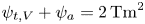 .
.

To the authors’ knowledge, no analytical solution to (2.4) and (2.5) exists in this geometry. The verification is thus carried out as follows. First, a rotational transform constraint case is run with an input ${\raise.3pt-\kern-5pt\iota}$ -profile that is chosen to be $10\,\%$
 larger than the vacuum rotational transform ${\raise.3pt-\kern-5pt\iota} _{\textrm {vac}}$
 , i.e. ${\raise.3pt-\kern-5pt\iota} = 1.10\times {\raise.3pt-\kern-5pt\iota} _{\textrm {vac}}$
 , so that there is a non-zero contribution from the current to the rotational transform. The volume and surface currents are evaluated from the obtained equilibrium and used to run a current constraint calculation to obtain a second equilibrium. The same initial guess for the geometry and the interfaces is used for both calculations. The rotational transform profile $\bar {{\raise.3pt-\kern-5pt\iota} }$
 is then extracted from the second equilibrium and compared with the reference ${\raise.3pt-\kern-5pt\iota}$
 -profile.
The vacuum rotational transform profile, as well as the profiles ${\raise.3pt-\kern-5pt\iota}$ and $\bar {{\raise.3pt-\kern-5pt\iota} }$
 are shown in figure 9(a). The toroidal current enclosed by the plasma is mostly contained in the volumes and adds up to a total of ${\sim }2.7\ \textrm {kA}$
 , see figure 9(b). As expected the surfaces currents $I^s_{\phi ,l}$
 remain small ($<10^{-2}\ \textrm {kA}$
 ), since there are no pressure gradients to drive them. The constraint on the rotational transform ${\raise.3pt-\kern-5pt\iota}$
 is enforced on each side of the volumes’ interfaces, indicated by grey dashed lines on figure 9(a). The value of ${\raise.3pt-\kern-5pt\iota}$
 at the computational boundary is not constrained. Agreement between ${\raise.3pt-\kern-5pt\iota}$
 and $\bar {{\raise.3pt-\kern-5pt\iota} }$
 up to a relative error of $\max (|{\raise.3pt-\kern-5pt\iota} -\bar {{\raise.3pt-\kern-5pt\iota} }| / |{\raise.3pt-\kern-5pt\iota} |)\sim 10^{-5}$
 is observed, showing that the same equilibrium can be obtained using either constraint. The maximum error between both profiles decreases as the numerical resolution is increased (data not shown).

Figure 9. (a) Rotational transform profile versus effective minor radius. Red triangles, ${\raise.3pt-\kern-5pt\iota}$ , input profile used in SPEC when run at fixed rotational transform; black dashed line, $\bar {{\raise.3pt-\kern-5pt\iota} }$
 , the output profile obtained from SPEC when run at fixed toroidal current profile; blue line, $\iota$
 -profile in vacuum; grey dashed lines, position of volume interfaces. (b) Total toroidal current enclosed by each volume. Surface currents (not plotted), $I^s_{\phi ,l}$
 , are smaller than $10^{-2}\ (\textrm {kA})$
 and are negligible in comparison with the volume current.
To verify the force gradient components, we use a fourth-order centred finite difference formula (Fornberg Reference Fornberg1988),

to obtain $\boldsymbol {\nabla } F_{FD}$ , i.e. a finite-difference estimate of the force gradient, and compare it with $\boldsymbol {\nabla } F$
 , i.e. the force gradient calculated in SPEC by using analytical derivatives. The finite difference estimate is evaluated by perturbing each geometrical degree of freedom $\{x_i\}_{l=1,\ldots ,N}$
 by a constant value $\Delta R$
 . Convergence as $\Delta R\rightarrow 0$
 is shown in figure 10. A convergence of order $O(\Delta R^4)$
 is observed down to $\sim 10^{-11}$
 for $\Delta R\sim 10^{-4}$
 . For lower values of $\Delta R$
 , the finite difference approximation error is dominated by round-off error. This shows that the analytical derivatives (the force gradient) are correctly implemented in SPEC.

Figure 10. Normalized maximum absolute error between SPEC force gradient and a finite difference estimate in the case of a rotating ellipse. The dashed line has slope of four.
5. Ideal equilibrium $\beta$ -limit in a classical stellarator

In this section, it is shown that the SPEC current constraint can be used to recover the HBS theory prediction of the classical stellarator ideal equilibrium $\beta$ -limit (Freidberg Reference Freidberg2014; Wakatani Reference Wakatani1998), when zero net toroidal current is considered.
A previous study (Loizu et al. Reference Loizu, Hudson, Nührenberg, Geiger and Helander2017) showed remarkable agreement between SPEC calculations and the HBS theory in a simplified case, with the pressure profile approximated by a single step. An additional limitation, enforced by the SPEC version at that time, was that the vacuum region had to be approximated by a large plasma volume where the pressure and currents were set to zero, and a fixed-boundary would be applied. This approach is equivalent to assuming a free-boundary calculation with an infinitely conducting wall at the computational boundary. At large $\beta$ , however, a strong Shafranov shift is present, and this approximation could have an impact on the result.
To understand the effect of these assumptions we consider here both fixed- and free-boundary calculations with a stepped-pressure profile approximating a Solov'ev's profile $p = p_0(1-\psi _t / \psi _a)$ where $\psi _a$
 is the total toroidal flux enclosed by the plasma. The computational boundary is defined by (4.1)–(4.2). Fixed-boundary calculations were made first, with seven plasma volumes surrounded by an eighth large, vacuum-like volume so that it is similar to a free-boundary calculation. The toroidal flux profile has been chosen such that $\psi _a=\sum _{l=1}^7\psi _{t,l}=0.25\,\text {Tm}^2$
 and $\psi _{t,8} = 0.75\,\text {Tm}^2$
 , leading to a total toroidal flux enclosed by the plasma and the vacuum-like region of $\sum _{l=1}^8\psi _{t,l} = 1\,\text {Tm}^2$
 . Free-boundary input files were generated to replicate the same equilibrium in vacuum, using $\mu _0I_{\textrm {coil}}=21.43\,\textrm {Tm}$
 and $\psi _a=0.25\,\text {Tm}^2$
 , which correspond to an equilibrium with $\psi _{t,V}=0.75\,\text {Tm}^2$
 . In both fixed- and free-boundary calculations, both the surface currents and the volume currents were set to zero, i.e. $I_{\phi ,l}^{\textrm {vol}} = I_{\phi ,l}^{\textrm {surf}} = 0$
 for all $l$
 . The only control parameter remaining is $p_0$
 , which was increased in order to increase the plasma average $\beta$
 until a central $m=1,\ n=0$
 island opens. The island emerges when the rotational transform at the plasma edge, ${\raise.3pt-\kern-5pt\iota} _a$
 , i.e. the rotational transform on the outer side of the plasma–vacuum interface, reaches zero (see figure 11). This is defined as the ideal equilibrium $\beta$
 -limit.

Figure 11. Poincaré plot of the magnetic field lines at $\phi =0$ and at three different values of $\langle \beta \rangle$
 (a–c). Red surfaces are the volume interfaces and the black, bold surface is the computational boundary. In panel (c), the ideal equilibrium $\beta$
 -limit has been exceeded and a central island opened outside the plasma. A large value of $\langle \beta \rangle$
 has been selected for illustration purposes. Here (a) ($\langle \beta \rangle = 0\,\%$
 , ${\raise.3pt-\kern-5pt\iota} _a\approx 0.28$
 ); (b) ($\langle \beta \rangle \approx 0.31\,\%$
 , ${\raise.3pt-\kern-5pt\iota} _a\approx 0.13$
 ); (c) ($\langle \beta \rangle \approx 0.62\,\%$
 , ${\raise.3pt-\kern-5pt\iota} _a= 0.0$
 ).
).
The physical mechanisms leading to the emergence of a separatrix are complex. In brief, the combination of non-zero poloidal harmonics of the Pfirsch–Schlüter and diamagnetic currents at the volumes’ interfaces and the effect of the Shafranov shift perturbs sufficiently the poloidal magnetic field so that the rotational transform at the plasma edge decreases, until eventually it reaches zero. These results will be explained in more detail in a future publication.
The HBS theory, building on the pioneering work of Greene and Johnson's stellarator expansion theory (Greene & Johnson Reference Greene and Johnson1961), predicts that

with ${\raise.3pt-\kern-5pt\iota} _v$ the rotational transform at the plasma edge in vacuum and ${\raise.3pt-\kern-5pt\iota} _I$
 a contribution from the plasma toroidal current,

with $I_\phi$ the total toroidal plasma current, $B_0$
 the magnetic field strength on axis and $a$
 the effective minor radius at the plasma edge, i.e. $a=\sqrt {\psi _a / (\psi _a + \psi _{t,V})} r_{\textrm {eff}}$
 , with $r_{\textrm {eff}}$
 the effective radius of the ellipse, given by the square root of the product between the ellipse major radius $r_{\textrm {max}}=|R_{10}+R_{11}|$
 and the ellipse minor radius $r_{\textrm {min}}=|Z_{10}+Z_{11}|$
 , i.e. $r_{\textrm {eff}}=\sqrt {r_{\textrm {max}}r_{\textrm {min}}}$
 . The parameter $\nu$
 is defined as

with $\langle \beta \rangle$ the volume averaged plasma $\beta$
 and $\epsilon _a = a / R_{00}$
 . Setting ${\raise.3pt-\kern-5pt\iota} _a=0$
 in (5.1) and solving for $\langle \beta \rangle$
 leads to a prediction for the ideal equilibrium $\beta$
 -limit,

In the case of interest, $R_{00}=10\ \textrm {m}$ , $R_{10}=-Z_{10}=1\ \textrm {m}$
 , $R_{11}=Z_{11}=0.25\ \textrm {m}$
 , leading to $r_{\textrm {eff}}\approx 0.97\ \textrm {m}$
 and $a\approx 0.48\ \textrm {m}$
 . Using $I_\phi =0$
 A and ${\raise.3pt-\kern-5pt\iota} _v\approx 0.28$
 , one obtains $\langle \beta \rangle _{\textrm {lim},\textrm {HBS}}\approx 0.38\,\%$
 .
.
Figure 12 shows the rotational transform profile at different values of $\langle \beta \rangle$ (figure 12a) and the values of ${\raise.3pt-\kern-5pt\iota} _a$
 obtained with SPEC as a function of $\langle \beta \rangle$
 and compares them with the analytical prediction given by (5.1) (figure 12b). Good agreement is observed between the fixed-boundary and free-boundary calculations, showing that the fixed-boundary assumption made by Loizu et al. (Reference Loizu, Hudson, Nührenberg, Geiger and Helander2017) has only a small effect on the ideal equilibrium $\beta$
 -limit prediction. In addition, the free-boundary calculation and the HBS theory agree well, and predict approximately the same ideal equilibrium $\beta$
 -limit. The small but finite difference between the results is most likely due to the HBS theory, which employs an expansion in aspect ratio $\epsilon$
 and assumes that the plasma boundary is circular. In fact, the number of volumes used in SPEC to approximate the continuous pressure profile does not significantly influence the result of this study (data not shown).

Figure 12. (a) Rotational transform profile at three different values of $\langle \beta \rangle$ , for free-boundary calculation of a rotating ellipse with zero net toroidal current. (b) Rotational transform at the plasma edge as a function of $\langle \beta \rangle$
 . Comparison between free-, fixed-boundary and the HBS theory.
As a final remark, note that in our calculations, the plasma boundary is topologically constrained to be an ideal surface and cannot undergo reconnection. Another important constraint is that the pressure profile is fixed and cannot evolve. Other approaches without these constraints could lead to different results and conclusions. One natural question is then to ask about the physical validity of constraining the topology of a set of flux surfaces in MRxMHD. First studies about the existence of MRxMHD interfaces have been carried out (McGann et al. Reference McGann, Hudson, Dewar and Von Nessi2010; Qu et al. Reference Qu, Hudson, Dewar, Loizu and Hole2021), pointing towards certain existence criteria. The present study, however, aims at verifying the implementation of the toroidal current constraint in SPEC by retrieving well-established mathematical results. Future work will focus on code validation by using experimental data.
6. Conclusion
Toroidal currents in MRxMHD have been derived and expressed in terms of simple quantities. Two profiles have been identified: the volume current profile, flowing through the volumes; and the surface current profile, flowing at each volume interface. A physical interpretation has been given for each of the currents. Both profiles have been implemented as new constraints in the SPEC code, which can now compute MRxMHD equilibria for a given toroidal current profile. Analytical derivatives of the force on each volume interface with respect to the interfaces’ geometry at fixed toroidal current have been derived and implemented in SPEC. These derivatives speed up substantially the Newton iterations on the interface geometries.
Both the new constraint and the force gradient implementation have been verified in slab, cylindrical and toroidal geometries. We presented in this paper only the latter two. In cylindrical geometry, we considered an axisymmetric screw pinch, where the obtained equilibria and force gradient could be compared with analytical solutions. In toroidal geometry, a classical stellarator geometry has been considered. The equilibrium has been verified to match the equilibrium obtained by constraining the rotational transform profile in SPEC, and the force gradient has been compared with a finite difference estimate.
Finally, the calculation of the ideal equilibrium $\beta$ -limit in a classical stellarator with zero net toroidal current has been presented as a first application of the new SPEC capabilities. The free-boundary calculation showed very good agreement both with a previous, simpler study (Loizu et al. Reference Loizu, Hudson, Nührenberg, Geiger and Helander2017) and with the HBS theory (Wakatani Reference Wakatani1998; Freidberg Reference Freidberg2014). In the future, the effect of bootstrap current on the equilibrium $\beta$
 -limit in a classical stellarator will be investigated. Furthermore, this new tool opens the possibility of comparing SPEC with previous results obtained with other equilibrium codes such as PIES (Drevlak et al. Reference Drevlak, Monticello and Reiman2005; Hirsch et al. Reference Hirsch, Baldzuhn, Beidler, Brakel, Burhenn, Dinklage, Ehmler, Endler, Erckmann and Feng2008), and perform similar studies on present experiments such as W7-X. In particular, it is envisaged to study W7-X equilibrium $\beta$
 -limits and its robustness to fluctuations in the toroidal current profile.
Acknowledgements
The authors acknowledge useful discussion with S.R. Hudson, C. Smiet, J. Schilling, J. Geiger and C. Zhu. The authors would also like to thank the referees for very careful reading and helpful constructive comments.
Editor Per Helander thanks the referees for their advice in evaluating this article.
Funding
This work has been carried out within the framework of the EUROfusion Consortium and has received funding from the Euratom research and training program 2014–2018 and 2019–2020 under grant agreement no. 633053. The views and opinions expressed herein do not necessarily reflect those of the European Commission (A.B., J.L., J.P.G.). This work is partly funded by Australian ARC projects DP170102606 (Z.Q., A.K.). This work was also supported by a grant from the Simons Foundation/SFARI (560651, AB) (A.B., J.L., Z.Q., A.K.).
Declaration of interests
The authors report no conflict of interest.
Appendix A
In this appendix we show the linear relation between the surface currents (2.7) and the poloidal fluxes. We rewrite here (2.7) for convenience,

We use general coordinates notation, with $u^i\equiv \{s,\theta ,\phi \}$ , $\{\boldsymbol {\nabla } s,\boldsymbol {\nabla }\theta ,\boldsymbol {\nabla }\phi \}$
 the contravariant basis and $\boldsymbol {e_i}\equiv \{\boldsymbol {e_s},\boldsymbol {e_\theta },\boldsymbol {e_\phi }\}$
 the covariant basis. This derivation is local to a volume and we drop the subscript $l$
 everywhere for simplicity.
We first show that the surface currents depend linearly on the vector potential degrees of freedom $\boldsymbol {a}$ . The contravariant components of the magnetic field are obtained from $\boldsymbol {\nabla }\times \boldsymbol {A}=\boldsymbol {B}$
 ,
,

where $\epsilon ^{ijk}$ is the Levi–Civita tensor, $\sqrt {g}$
 is the Jacobian, and the Einstein summation convention has been used. The covariant component of the magnetic field can then easily be expressed by $B_\theta = g_{k\theta }B^k$
 . The $m=n=0$
 Fourier mode of $B_\theta$
 is then

with $S$ the total area of the flux surface, which depends only on geometrical quantities. Derivatives of $A_j$
 are
are


where the prime denotes the derivative with respect to the main argument. Equations (A3) and (A4)–(A6) combined show the linear dependence of $\tilde {B}_\theta$ on $\boldsymbol {a}$
 . Finally, the Beltrami equation (3.6) provides a linear relation between $\boldsymbol {a}$
 and $\{\psi _p,\psi _t,\mu \}$
 . All relations being linear, this shows that the surface currents depend linearly on the poloidal and toroidal magnetic fluxes.
Appendix B
In this appendix, the main differences between a fixed- and free-boundary calculation with the new developed current constraint are outlined. The linear system (3.11) has to be rewritten by extending the arrays $\boldsymbol {\psi }$ and $\boldsymbol {I}$
 with two new pairs of scalars $(\psi _{p,V}, \psi _{t,V})$
 and ($I^s_{N_{\textrm {vol}}}, I_{\textrm {coil}}$
 ), namely $\boldsymbol {\psi }\equiv (\psi _{p,2},\ldots ,\psi _{N_{\textrm {vol}}}, \psi _{p,V}, \psi _{t,V})^t$
 and $\boldsymbol {I}\equiv (I^s_1,\ldots ,I^s_{N_{\textrm {vol}}},I_{\textrm {coil}})^t$
 . Then,

with the matrix $\boldsymbol {M}_{\textrm {Fr}}$ ,
,

with $\tilde {B}^-_{\phi ,V}$ the $m=n=0$
 Fourier mode of the covariant toroidal magnetic field on the plasma boundary outer side. Regarding (3.15), no changes are needed in the plasma volumes. In the vacuum region, however, the toroidal flux is not fixed and an additional term is needed,

where the subscript $V$ denotes the vacuum region.
Regarding the force gradient, the derivative of the toroidal flux with respect to the geometry is non-zero in the vacuum region. This means that

An additional equation is required for ${\textrm {d}\psi _{t,V}}/{\textrm {d}x_i}$ , and is provided by

leading to

Appendix C
The solution to the Beltrami equation (2.4) in the $l{\text {th}}$ volume of an axisymmetric cylinder is

where the usual $(r,\theta ,\phi )$ cylindrical coordinate system has been used, $\textrm {J}_i$
 and $\textrm {Y}_i$
 are the Bessel functions of the $i$
 th order of the first and second kind, respectively, and $c_{l,1}$
 , $c_{l,2}$
 are integration constants. Here $\boldsymbol {\nabla }\theta$
 and $\boldsymbol {\nabla }\phi$
 are the contravariant basis vectors.
In addition, since $B_\theta$ must vanish at the origin, we have that $c_{1,2}=0$
 . Indeed, the asymptotic expansion of $\textrm {Y}_1(x)$
 close to $x=0$
 gives (Abramowitz & Stegun Reference Abramowitz and Stegun1972)

which is only zero if $c_{1,2}=0$ .
.
We consider now the case of a screw pinch with three inner volumes, $N_{\textrm {vol}}=3$ . The assumed constrained profiles are the toroidal flux $\{\psi _{t,l}\}_{l=1,2,3}$
 , the volume current $\{I^{v}_{l,\phi }\}_{l=1,2,3}$
 and the surface current $\{I^{s}_{l,\phi }\}_{l=1,2}$
 . The constraint on the toroidal flux is


where $\sqrt {g}=r$ is the Jacobian and $S_{l,\phi }$
 is a constant-$\phi$
 surface in volume $l$
 . The Bessel function integrals have been renamed as $\bar {\textrm {J}}_l$
 and $\bar {\textrm {Y}}_l$
 , and $R_l$
 is the radius of the $l{\text {th}}$
 interface. The constraints on the currents lead to


Solving for $\{c_{l,1},c_{l,2}\}$ is equivalent to solving the linear system

Derivatives of the force $F_l= [(B_{l+1}(R_l))^2-(B_l(R_l))^2] / 2$ can also be expressed analytically, leading to

with $l,j\in \{1,2\}$ . Consider, e.g. the derivative of $B_l(R_k),\ k=\{l-1,l\}$
 ,
,


where the $'$ denotes a derivative with respect to the function argument, and all Bessel functions are evaluated at $\mu _lR_k$
 . Finally, all derivatives must be taken at constant $\psi _{t,l}$
 , $I^{\textrm {v}}_{l,\phi}$
 and $I^{{s}}_{l,\phi}$
 . In particular, the coefficients ${\textrm {d}c_{l,i}}/{\textrm {d}R_k}$
 are obtained from derivatives of (C8) with respect to $R_k$
 .
.


 Open access