


1 Introduction and motivation
Energetic particles (EP) are ubiquitous in both laboratory and astrophysical plasmas. By definition, they exhibit velocities much larger than the thermal velocity of the bulk plasma, which is characterised by a Maxwellian distribution function. EP, such as the alpha particles, must be sufficiently well confined in order to transfer their energy to the bulk plasma through Coulomb collisions or to ensure the current drive efficiency (Heidbrink & Sadler Reference Heidbrink and Sadler1994; Sharapov et al. Reference Sharapov, Alper, Borba, Eriksson, Fasoli, Gill, Gondhalekar, Gormezano, Heeter and Huysmans2000; Pinches et al. Reference Pinches, Berk, Borba, Breizman, Briguglio, Fasoli, Fogaccia, Gryaznevich, Kiptily and Mantsinen2004). Nevertheless, due to the curvature of the magnetic field lines, the trajectories of particles depart from the magnetic flux surfaces. This departure (called magnetic drift) is more pronounced when the energy of particles increases. Therefore, the magnetic drift of EP can be intense enough so that their trajectories intercept the wall even with circular concentric magnetic surfaces, leading to losses and limiting the performance of the machine. In addition, the presence of a substantial population of particles at high energies leads to gradients in phase space, which may result in instabilities called energetic particle modes (EPM) (see for instance Chen & Zonca (Reference Chen and Zonca2007), Heidbrink (Reference Heidbrink2008), Lauber (Reference Lauber2013) and Chen & Zonca (Reference Chen and Zonca2016) and references therein). EPM tend to increase the transport of energetic particles, reducing inevitably the tokamak performance. Therefore, understanding and controlling the EPMs is also of prime importance for the future of ITER. In the presence of fluctuations driven by EP, such as for toroidal Alfvén eigenmodes, zonal structures can be nonlinearly generated (Chen & Zonca Reference Chen and Zonca2012). Direct excitation of zonal structures by EP is also possible, which occurs in the context of a special class of EPMs called energetic geodesic acoustic modes (EGAMs), dominated by a zonal structure  $(m,n)=(0,0)$ oscillating approximately at the acoustic frequency (Fu Reference Fu2008; Nazikian et al. Reference Nazikian, Fu, Austin, Berk, Budny, Gorelenkov, Heidbrink, Holcomb, Kramer and McKee2008; Qiu, Zonca & Chen Reference Qiu, Zonca and Chen2010; Zarzoso et al. Reference Zarzoso, Garbet, Sarazin, Dumont and Grandgirard2012). Because EGAMs are axisymmetric modes, they were initially believed not to play a significant role in the transport of particles. Nonetheless, it was experimentally and numerically evidenced that losses can occur in the presence of these axisymmetric large scale modes (Nazikian et al. Reference Nazikian, Fu, Austin, Berk, Budny, Gorelenkov, Heidbrink, Holcomb, Kramer and McKee2008; Fisher et al. Reference Fisher, Pace, Kramer, Van Zeeland, Nazikian, Heidbrink and García-Muñoz2012). It was in particular shown that most of these losses are due to chaotic transport in phase space (Zarzoso et al. Reference Zarzoso, del-Castillo-Negrete, Escande, Sarazin, Garbet, Grandgirard, Passeron, Latu and Benkadda2018), but so far no systematic studies of the nature of transport in the presence of EGAMs have been carried out. Similarly, zonal structures can be driven by drift-wave turbulence in magnetised plasmas (Hasegawa, Maclennan & Kodama Reference Hasegawa, Maclennan and Kodama1979) and play a major role in the regulation of micro-turbulence-induced transport in tokamaks (Lin et al. Reference Lin, Hahm, Lee, Tang and White1998). Although studies of the EP transport in the presence of micro-turbulence have been performed in the past (Zhang, Lin & Chen Reference Zhang, Lin and Chen2008; Angioni et al. Reference Angioni, Peeters, Pereverzev, Bottino, Candy, Dux, Fable, Hein and Waltz2009; Hauff et al. Reference Hauff, Pueschel, Dannert and Jenko2009; Zhang, Lin & Chen Reference Zhang, Lin and Chen2011; Pace et al. Reference Pace, Austin, Bass, Budny, Heidbrink, Hillesheim, Holcomb, Gorelenkova, Grierson and McCune2013; Bovet et al. Reference Bovet, Fasoli, Ricci, Furno and Gustafson2015), the direct impact of zonal structures on the EP transport remains unexplored. Therefore, we aim in this work to shed light on the fundamental mechanisms responsible for the EP transport in the presence of zonal structures. For this purpose, statistical analyses can be performed to determine some characteristic properties of the transport and the anomalous losses of EP. By anomalous losses we mean losses that do not follow the loss rate of a diffusive process. As we will explain, one of the main contributions of this work is to show that these anomalous losses are due to the presence of super-diffusive poloidal transport. In this paper, we focus our analyses on the transport induced by zonal structures in the context of EGAMs, but the results can be extended without any loss of generality to situations where zonal structures are nonlinearly generated by small amplitude perturbations. The remainder of the paper is structured as follows. Section 2 presents the model we use for the statistical analysis. In § 3 we present the observations of fractal-like behaviour and algebraic decay of the exit time of EP using relevant tokamak parameters. This naturally leads to § 4, where we give, for the first time, evidence that zonal structures can lead to anomalous diffusion of energetic particles. Conclusions and future work are presented in § 5.
2 Description of the model
Within the framework of the EGAM-induced transport, we base our analysis on previous results obtained with gyro-kinetic simulations (Zarzoso et al. Reference Zarzoso, del-Castillo-Negrete, Escande, Sarazin, Garbet, Grandgirard, Passeron, Latu and Benkadda2018). However, in order to have meaningful statistical analyses, we need to simulate a huge number of test particles during sufficiently long gyro-kinetic simulations. Due to computational restrictions, we avoid this approach by replacing the EGAM potential obtained from the expensive direct gyro-kinetic simulations by an analytical model containing the main physics of the EGAM. This strategy is the most favorable in terms of CPU time, since no interpolation of the field is required. In addition, it allows us to simulate trajectories on time scales comparable with the experimental measurements. The main characteristics of a zonal ( $n=0$) structure are: (i) its frequency, (ii) its spatial (radial and poloidal) structure and (iii) its amplitude. A zonal structure can therefore be modelled as
 $$\begin{eqnarray}\unicode[STIX]{x1D719}(r,\unicode[STIX]{x1D703},t)\approx [\unicode[STIX]{x1D719}_{00}(r)+\unicode[STIX]{x1D719}_{10}(r)\sin \unicode[STIX]{x1D703}]\cos (\unicode[STIX]{x1D714}t),\end{eqnarray}$$
 where  $\unicode[STIX]{x1D719}$ is the potential, decomposed here into its Fourier modes ( $\unicode[STIX]{x1D719}_{00}$ for ( $m=0$, $n=0$) and $\unicode[STIX]{x1D719}_{10}$ for ( $m=1$, $n=0$)), $r$ is the radial position represented by the tokamak minor radius, $\unicode[STIX]{x1D703}$ is the poloidal angle, $\unicode[STIX]{x1D714}$ is the frequency and $t$ is the time.
Based on the ordering  $\unicode[STIX]{x1D719}_{10}\sim 10^{-1}\unicode[STIX]{x1D719}_{00}$, we neglect in the following the poloidal dependence and focus only on the dominant component. Following gyro-kinetic simulations (Zarzoso et al. Reference Zarzoso, Garbet, Sarazin, Dumont and Grandgirard2012, Reference Zarzoso, Sarazin, Garbet, Dumont, Strugarek, Abiteboul, Cartier-Michaud, Dif-Pradalier, Ghendrih and Grandgirard2013, Reference Zarzoso, Migliano, Grandgirard, Latu and Passeron2017) we can model the radial dependence as
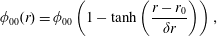 $$\begin{eqnarray}\unicode[STIX]{x1D719}_{00}(r)=\unicode[STIX]{x1D719}_{00}\left(1-\tanh \left(\frac{r-r_{0}}{\unicode[STIX]{x1D6FF}r}\right)\right),\end{eqnarray}$$
 where  $\unicode[STIX]{x1D719}_{00}$ is the value of the potential at $r=r_{0}$ and $\unicode[STIX]{x1D6FF}r$ controls the width of the mode. This gives a radial electric field of amplitude $E_{r,0}=\unicode[STIX]{x1D719}_{00}/\unicode[STIX]{x1D6FF}r$ at $r=r_{0}$ and localised in a region $r_{0}-\unicode[STIX]{x1D6FF}_{r}/2<r<r_{0}+\unicode[STIX]{x1D6FF}_{r}/2$.
The guiding-centre equations of motion to be solved in toroidal geometry in the presence of a given electrostatic potential are (Grandgirard et al. Reference Grandgirard, Abiteboul, Bigot, Cartier-Michaud, Crouseilles, Dif-Pradalier, Ehrlacher, Esteve, Garbet and Ghendrih2016)
 $$\begin{eqnarray}\displaystyle & \displaystyle \frac{\text{d}x^{i}}{\text{d}t}=v_{\Vert }\boldsymbol{b}^{\ast }\boldsymbol{\cdot }\unicode[STIX]{x1D735}x^{i}+\boldsymbol{v}_{E}\boldsymbol{\cdot }\unicode[STIX]{x1D735}x^{i}+\boldsymbol{v}_{D}\boldsymbol{\cdot }\unicode[STIX]{x1D735}x^{i}, & \displaystyle\end{eqnarray}$$
 $$\begin{eqnarray}\displaystyle & \displaystyle m_{s}\frac{\text{d}v_{\Vert }}{\text{d}t}=-\unicode[STIX]{x1D707}\boldsymbol{b}^{\ast }\boldsymbol{\cdot }\unicode[STIX]{x1D735}B-eZ_{s}\boldsymbol{b}^{\ast }\boldsymbol{\cdot }\unicode[STIX]{x1D735}J_{0}\unicode[STIX]{x1D719}+\frac{m_{s}v_{\Vert }}{B}\boldsymbol{v}_{E}\boldsymbol{\cdot }\unicode[STIX]{x1D735}B, & \displaystyle\end{eqnarray}$$ $x^{i}$ is the $i\text{th}$ contravariant component of the coordinate $\boldsymbol{x}$ ( $x^{1}\equiv r$ in the radial direction, $x^{2}\equiv \unicode[STIX]{x1D703}$ in the poloidal direction and $x^{3}\equiv \unicode[STIX]{x1D711}$ in the toroidal direction), $v_{\Vert }$ the parallel component of the velocity along the magnetic field lines, $\boldsymbol{v}_{E}$ is the $\boldsymbol{E}\times \boldsymbol{B}$ drift, $\boldsymbol{v}_{D}$ is the magnetic drift, $\unicode[STIX]{x1D707}$ is the magnetic moment, which is an invariant within the present model, $m_{s}$ is the mass of particles, $e$ is the elementary charge, $Z_{s}$ is the atomic number, $B$ is the magnitude of the magnetic field, $J_{0}$ is the gyro-average operator and $\boldsymbol{b}^{\ast }$ is defined as
  $$\begin{eqnarray}\boldsymbol{b}^{\ast }=\frac{\boldsymbol{B}}{B_{\Vert }^{\ast }}+\frac{m_{s}v_{\Vert }}{eZ_{s}B_{\Vert }^{\ast }B}\unicode[STIX]{x1D735}\times \boldsymbol{B},\end{eqnarray}$$
with
 $$\begin{eqnarray}B_{\Vert }^{\ast }=B+\frac{m_{s}}{eZ_{s}}v_{\Vert }\boldsymbol{b}\boldsymbol{\cdot }\unicode[STIX]{x1D735}\times \boldsymbol{b},\end{eqnarray}$$
 where  $\boldsymbol{b}$ is the unit vector along the magnetic field. This expression (2.5) allows us to write the volume element in guiding-centre velocity space as $(2\unicode[STIX]{x03C0}B_{\Vert }^{\ast }/m_{s})\,\text{d}v_{\Vert }\,\text{d}\unicode[STIX]{x1D707}$.
To further reduce the computational time, it is important to realise that due to the axisymmetry of the electrostatic potential, the equation for the toroidal angle does not need to be integrated to determine the radial transport. Axisymmetry also implies the conservation of the toroidal canonical momentum  $P_{\unicode[STIX]{x1D711}}$
 $$\begin{eqnarray}P_{\unicode[STIX]{x1D711}}=-eZ_{s}\unicode[STIX]{x1D713}+m_{s}v_{\unicode[STIX]{x1D711}}=\,\text{const.},\end{eqnarray}$$
 with  $v_{\unicode[STIX]{x1D711}}=b_{\unicode[STIX]{x1D711}}v_{\Vert }$, where $b_{\unicode[STIX]{x1D711}}$ is the toroidal covariant component of the unit vector along the magnetic field, $R$ is the major radius and $\unicode[STIX]{x1D713}$ is the poloidal flux, which is written for circular flux surfaces in terms of the safety factor $q$, the amplitude of the magnetic field at the magnetic axis $B_{0}$ and the radial position $r$ as
 $$\begin{eqnarray}\unicode[STIX]{x1D713}=B_{0}\int _{0}^{r}\frac{r^{\prime }}{q(r^{\prime })}\,\text{d}r^{\prime }.\end{eqnarray}$$
 Equation (2.6) allows us to obtain the parallel velocity  $v_{\Vert }$ at each time step without integrating equation (2.3b). Finally, for large scale zonal structure the gyro-average is not expected to play a major role. Therefore, we make the simplification $J_{0}\cdot \unicode[STIX]{x1D719}=\unicode[STIX]{x1D719}$. This numerical scheme reduces the number of differential equations to be integrated and ensures the exact conservation of the toroidal canonical momentum within machine precision. The differential equations for $r$ and $\unicode[STIX]{x1D703}$ are solved using a fourth-order Runge–Kutta explicit integration in time. Following a convergence test, the time step for all the simulations has been set up to $\unicode[STIX]{x0394}t=50$ normalised to the cyclotron period. In all the simulations presented in this paper, the safety factor is assumed to be flat and set to $q=1.8$, the width of the electrostatic potential is $\unicode[STIX]{x1D6FF}r=20\unicode[STIX]{x1D70C}_{\text{th}}$, which is larger than the maximum Larmor radius of the energetic particles that we consider, and the frequency is $\unicode[STIX]{x1D714}=3.7\times 10^{-3}$ normalised to the cyclotron frequency, which is typical of self-consistent gyro-kinetic simulations presented in Zarzoso et al. (Reference Zarzoso, del-Castillo-Negrete, Escande, Sarazin, Garbet, Grandgirard, Passeron, Latu and Benkadda2018).
3 Fractal-like dependence of loss time on initial conditions
Motion invariants are very valuable to describe how the trajectories are modified in the presence of a perturbation. This is because in the absence of any perturbation, a particle initialised with a given value of the invariants will explore the phase space while keeping the motion invariants constant, which translates into a one-dimensional (1-D) curve in the 3-D real space when three invariants exist. We know that this trajectory will correspond to the one of any other particle initialised in such a way that at  $t=0$ it has the same motion invariants. The unperturbed trajectory of a particle can for instance be described by the kinetic energy $E$ and the ratio between the magnetic moment and the kinetic energy, $\unicode[STIX]{x1D6EC}=\unicode[STIX]{x1D707}B_{0}/E$, providing the initial radial position is known. An example is illustrated in figure 1, where (a) represents the projection onto the poloidal cross-section of the trajectories of two particles, one deeply counter-passing and the other barely counter-passing, both starting at the radial position $r/a=0.1$ and the poloidal angle $\unicode[STIX]{x1D703}=0$ (fixing therefore $P_{\unicode[STIX]{x1D711}}$). Of course, particles are injected with a certain range of $E$ and $\unicode[STIX]{x1D6EC}$. If all the particles are injected roughly at the same position, the resulting trajectories will cover the area represented by the blue region in figure 1(b).

Figure 1. (a) Trajectories of two counter-passing particles: one deeply counter-passing with  $(\unicode[STIX]{x1D6EC}=0.4,E=25E_{\text{th}})$, represented by the almost circular projection, and one barely counter-passing with $(\unicode[STIX]{x1D6EC}=0.8,E=43E_{\text{th}})$. (b) Ensemble of all the possible trajectories with energies within the range $25E_{\text{th}}\leqslant E\leqslant 43E_{\text{th}}$ and pitch angle $0.4\leqslant \unicode[STIX]{x1D6EC}\leqslant 0.8$.
One can use then the electrostatic potential model in (2.1) to study the losses of particles injected in the inner region of the tokamak, at  $r/a\approx 0.1$ with a certain range of $E$ and $\unicode[STIX]{x1D6EC}$. It is to be noted that the adiabatic invariance of the magnetic moment $\unicode[STIX]{x1D707}$ is imposed owing to the gyro-kinetic ordering. In addition, since the modes are axisymmetric, the toroidal canonical momentum $P_{\unicode[STIX]{x1D711}}$ is an exact invariant, which is also imposed by solving (2.6). Regarding the kinetic energy, it remains invariant only if the perturbed potential does not depend explicitly on time. The fact that we have only two motion invariants of guiding centres in a system with three degrees of freedom makes it actually possible that the motion is chaotic, as reported in Zarzoso et al. (Reference Zarzoso, del-Castillo-Negrete, Escande, Sarazin, Garbet, Grandgirard, Passeron, Latu and Benkadda2018). We have performed a set of simulations for each couple $(E,\unicode[STIX]{x1D6EC})$ up to $t=2\times 10^{5}$ cyclotron periods. The result of this calculation is given in figure 2. Panel (a) shows the fraction of lost particles as a function of their initial kinetic energy and $\unicode[STIX]{x1D6EC}$, with iso-contours of the toroidal canonical momentum.
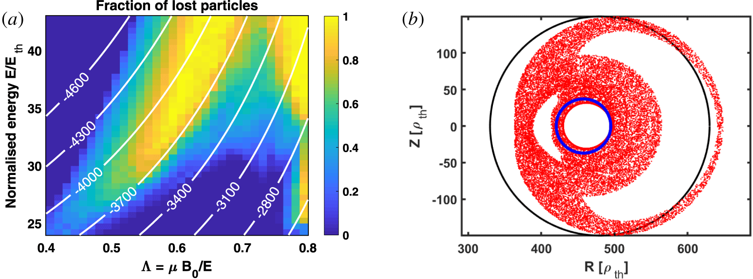
Figure 2. (a) Fraction of lost particles as a function of initial  $E$ and $\unicode[STIX]{x1D6EC}$ in the presence of a perturbation. The overlaid contours correspond to $P_{\unicode[STIX]{x1D711}}=\text{const}$. (b) Poincaré map of an initial condition with $\unicode[STIX]{x1D6EC}=0.54$ and $E=31.5E_{\text{th}}$ without perturbation (blue dots) and with perturbation (red dots).
When focusing on a particular point of figure 2(a), (for instance the one with initial  $\unicode[STIX]{x1D6EC}=0.54$ and $E=31.5E_{\text{th}}$, characterised by a lost fraction of approximately $0.8$), we can plot the invariant surface in the absence of the perturbation (blue circle) and the Poincaré map in the presence of the perturbation of the particles initialised on that blue circle. This is what figure 2(b) shows. This is a clear example of how an initially confined counter-passing particle can be lost due to the perturbation. The escape region is given by the intersection of the chaotic sea (red dots) with the tokamak wall (black circle), and depends on the initial conditions of the lost particle.
Figure 2(b) seems to indicate that all particles initialised on the blue circle should leave the domain, but figure 2(a) shows that only 80 % of the particles are lost. There are two complementary explanations for this issue, one numerical and another theoretical. Numerically, it should be kept in mind that all results pertain to finite-time dynamics, which for the simulations reported in figure 2(a) is  $2\times 10^{5}$ cyclotron periods. That is, figure 2(a) is the fraction of particles lost at or before $2\times 10^{5}$ cyclotron periods. There is also a theoretical aspect to this issue related to the fact that the red region in figure 2(b) does not have a trivial topology because (as it is common in Hamiltonian chaos) the Poincaré map of an orbit does not necessarily fill ergodically a simple 2-D manifold. Indeed, even if we were able to run a simulation for arbitrarily long time, we might find particles initialised in the blue circle that do not intercept the wall, despite the fact that the blue circle seems to be sort of embedded in the chaotic red region. There are also boundaries between the non-chaotic regions (e.g. the white islands where the red point did not enter) and the chaotic region (i.e. the region that contains the red points in the Poincaré map) separated by Cantor sets known as Cantori (see e.g. Meiss (Reference Meiss1992)) that trap particles and preclude them from escaping.
The observed chaotic motion implies that the trajectories of particles exhibit sensitive dependence on initial conditions. It is thus expected that the exit time of the lost particles also exhibits sensitive dependence on initial conditions. Analysing this dependence is especially relevant, since it allows us to identify the existence of patterns or structures. This cannot be done with diagrams of lost particles as those reported in Zarzoso et al. (Reference Zarzoso, del-Castillo-Negrete, Escande, Sarazin, Garbet, Grandgirard, Passeron, Latu and Benkadda2018), because the quantity plotted there was binary (either the particle is lost or it remains confined). Of course, since the exit time of particles that are never lost is infinite, the best way to represent the exit time is by plotting its inverse, i.e.  $t_{\text{exit}}^{-1}$. Figure 3 shows the inverse of the exit time as a function of the initial parallel velocity and magnetic moment. Panel (a) shows $t_{\text{exit}}^{-1}$ for all the simulated initial conditions. A clear pattern of structures aligned with the trapping cone is observed. To unveil the detailed structure of the dependence of $t_{\text{exit}}^{-1}$ on $v_{\Vert }$ and $\unicode[STIX]{x1D707}$, panels (b,c) show successive zooms, revealing similar structures at smaller scales when focusing on the region of lost particles. It is to be noted that, although the successive zooms do not exhibit exact self-similarity, it is clear that there is a non-trivial dependence of the exit time on initial conditions at all scales, what we refer to as fractal-like behaviour. The observed property of scale invariance imply similarity properties that can be uncovered when performing statistical analysis of the particle dynamics.
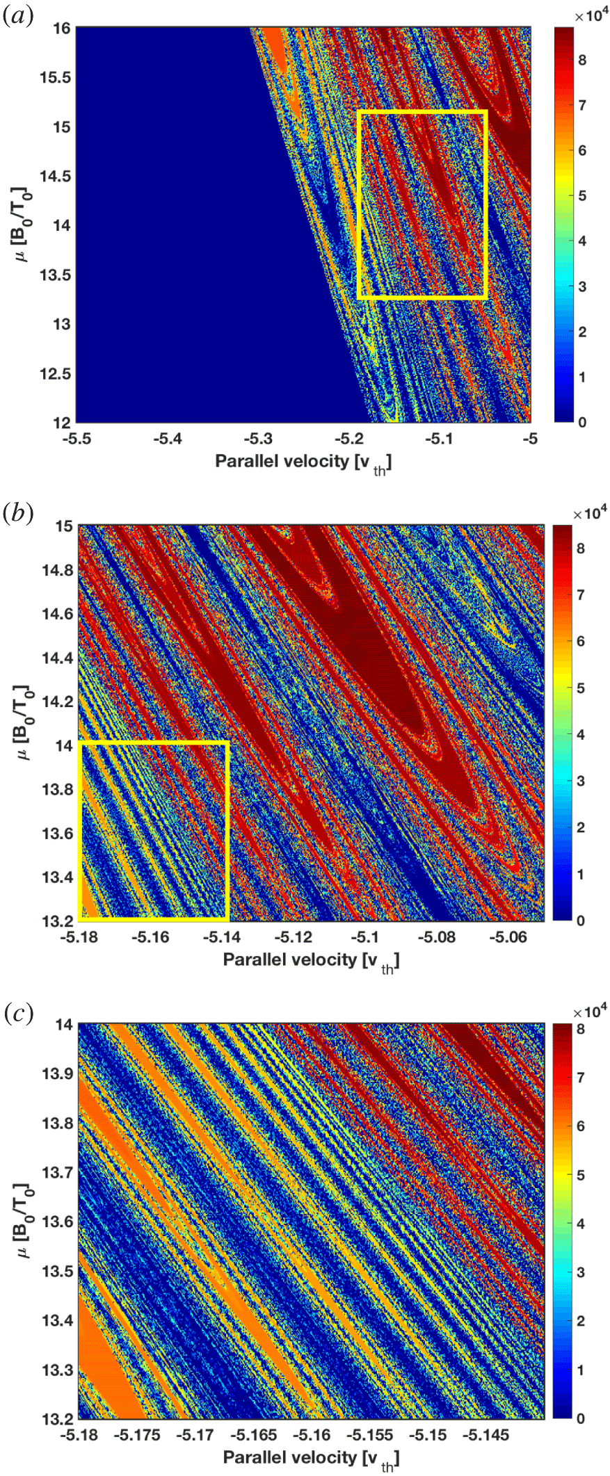
Figure 3. Inverse of the exit time as a function of the initial parallel velocity and magnetic moment. The middle and bottom panels show successive zooms of the  $(v_{\Vert },\unicode[STIX]{x1D707})$ parameter space, illustrating the same structures at smaller scales.
We can now focus the analysis on a more restricted region in velocity space, selecting almost mono-energetic EP injected in a localised region of the tokamak and determining the probability distribution function (PDF) of their exit time. We assume experiment-relevant parameters, taking the minor radius of the tokamak ( $a$) and the thermal ion Larmor radius ( $\unicode[STIX]{x1D70C}_{\text{th}}$) such that $\unicode[STIX]{x1D70C}_{\star }=1/150$, with $\unicode[STIX]{x1D70C}_{\star }=\unicode[STIX]{x1D70C}_{\text{th}}/a$, and we calculate the exit time of an ensemble of counter-passing EP. Such EP are characteristic of neutral beam injection (NBI) heating in medium-size tokamaks like DIII-D. For this purpose, we follow ${\sim}4\times 10^{5}$ deuterium tracers initialised at the position $r=0.4a$, $\unicode[STIX]{x1D703}=0$, $\unicode[STIX]{x1D711}=0$, with energy $E\approx 20E_{\text{th}}$ and magnetic moment such that $\unicode[STIX]{x1D707}B_{0}/T_{i}=14$. These particles are confined in the absence of any perturbation. We use Gysela normalisations (Grandgirard et al. Reference Grandgirard, Abiteboul, Bigot, Cartier-Michaud, Crouseilles, Dif-Pradalier, Ehrlacher, Esteve, Garbet and Ghendrih2016), but one can recover the units by choosing parameters for standard tokamaks. For instance, with $T_{i}\approx 4~\text{keV}$ and $B_{0}\approx 2~\text{T}$, one gets $a\approx 0.67~\text{m}$, which is typical of medium-size tokamaks. Using the amplitude of the EGAM in nonlinear Gysela simulations ( $\unicode[STIX]{x1D719}_{00}=1.5$), and using the electron temperature $T_{e}\approx 3~\text{keV}$, the amplitude of the radial electric field is $E_{r,0}\approx 14~\text{kV}~\text{m}^{-1}$, which is of the same order as the one obtained in Fisher et al. (Reference Fisher, Pace, Kramer, Van Zeeland, Nazikian, Heidbrink and García-Muñoz2012). Despite the simple structure of $\unicode[STIX]{x1D719}$, its time dependence leads to radial transport and losses. The PDF of the exit time, ${\mathcal{P}}_{\text{exit}}$, is plotted in figure 4 in log–log scale, showing an algebraic decay ${\mathcal{P}}_{\text{exit}}\sim t^{-\unicode[STIX]{x1D707}_{e}}$, in contrast with the exponential decay one would expect in the case of a diffusive transport (Gardiner Reference Gardiner2004). For the parameters chosen here, the tail of the PDF is developed from 1 to 100 ms. It is to be noted that a long time decay was mentioned in Fisher et al. (Reference Fisher, Pace, Kramer, Van Zeeland, Nazikian, Heidbrink and García-Muñoz2012), although no scaling was provided.
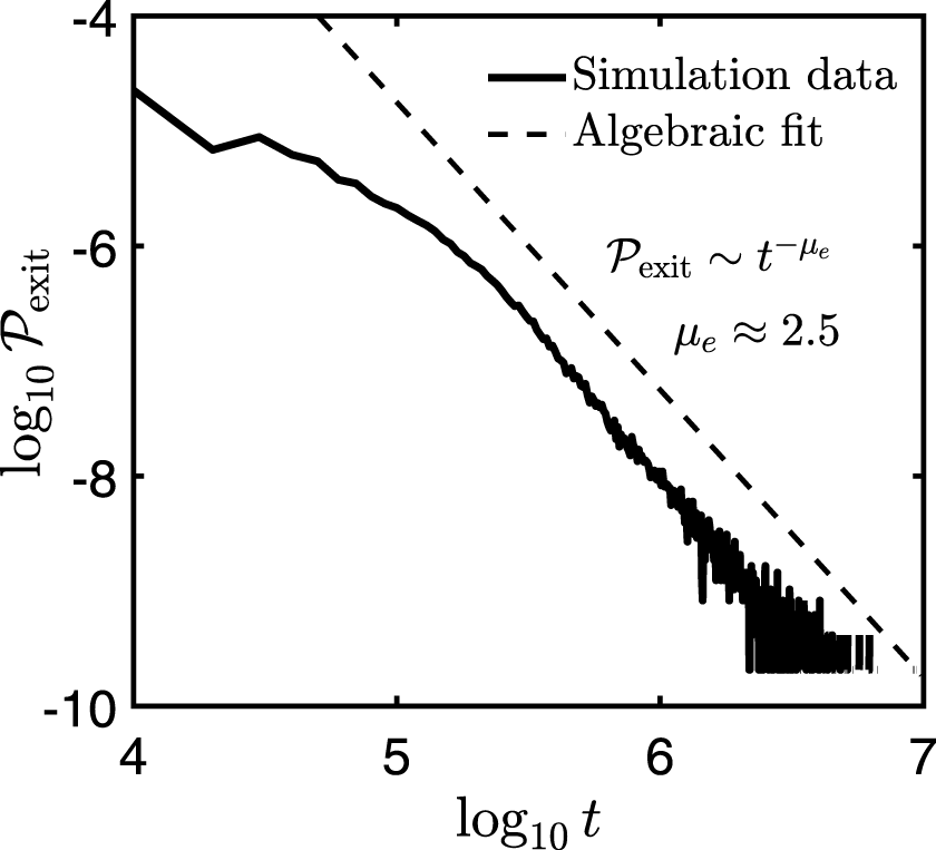
Figure 4. Probability distribution function of the exit time for counter-passing EP initialised at  $r=0.4a$, $\unicode[STIX]{x1D703}=0$, $\unicode[STIX]{x1D711}=0$, with $E=20E_{\text{th}}$ and $\unicode[STIX]{x1D707}B_{0}/T_{i}=14$. The dashed line shows an algebraic fit, with $\unicode[STIX]{x1D707}_{e}=2.5$.
To compare with the expected result in the case of diffusive behaviour, we can perform a simple exercise where we consider the motion of an ensemble of particles initially located at  $(x,y)=(0,0)$ on a 2-D disk. The two physical parameters in this simple model are the diffusivity, $D$, and the radius of the circle, $R_{c}$. Figure 5 shows the probability of the exit time for different values of $R_{c}$ and $D$ according to a Monte Carlo simulation of the diffusion equation on a disk. For all values of $R_{c}$ and $D$ the probability exhibits an exponential decay of the form
 $$\begin{eqnarray}P_{\text{diff}}\sim T_{\text{mean}}\exp [-\unicode[STIX]{x1D706}t/T_{\text{mean}}],\end{eqnarray}$$
 where  $\unicode[STIX]{x1D706}\approx 3/2$ and $T_{\text{mean}}$ is the mean exit time (first moment) for particles under the Brownian motion on a disk,
 $$\begin{eqnarray}T_{\text{mean}}=\frac{\unicode[STIX]{x03C0}R_{c}^{2}}{4D}.\end{eqnarray}$$
 It is interesting to point out that, because in figure 4 we get  $\unicode[STIX]{x1D707}_{e}>2$, the mean exit time does exists. However, the second moment, is infinite and thus not defined. This is in stark contrast with the diffusion problem for which all the moments of the exit time distribution exist.
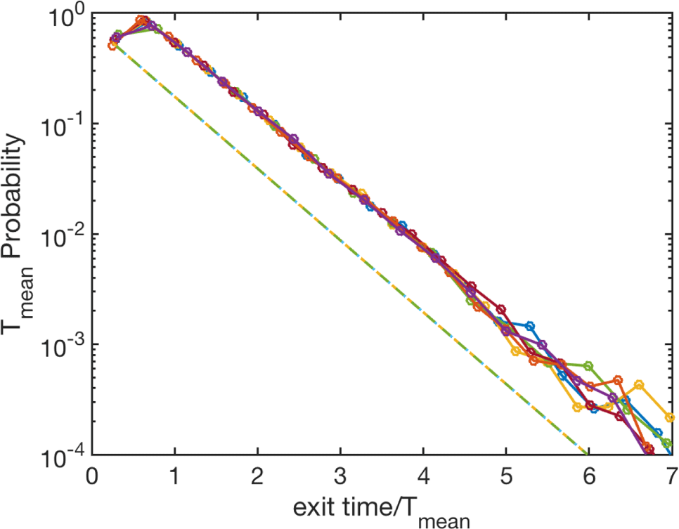
Figure 5. Monte Carlo simulation of exit time for an ensemble of particles initialised at  $(x,y)=(0,0)$ on a disk of radius $R_{c}$ in the presence of a diffusivity $D$. The plot shows the probability dependence on time rescaled by the analytical mean exit time $T_{\text{mean}}$ in (3.2) for $(R_{c},D)=\{(0.1,1),(1,0.1),(1,10)\,(2,1)\,(10,1)\,(1,1)\}$. The dashed line shows an exponential fit with decay rate $\unicode[STIX]{x1D706}=3/2$.
To understand why this algebraic decay occurs and therefore why the radial transport is not diffusive in the presence of an oscillating radial electric field, we focus on the region responsible for the chaotic transport of particles, i.e. the stochastic layer separating the passing and trapped particles. Let us remember that, in the absence of any perturbation, the particles in a tokamak are divided into trapped and passing and the boundary between these two classes is called trapping cone. This cone is a well-defined surface in phase space, also called the separatrix, since it represents the separation between the two classes of particles. The black lines in figure 6 represent the Poincaré map of the unperturbed trajectories for passing and trapped particles. Panel (a) represents the projection onto the poloidal cross-section, i.e. onto the  $(R,Z)$ sub-space, and panel (b) represents the projection onto the $(r^{2}/2,\unicode[STIX]{x1D703})$ sub-space. The dashed blue lines with arrows in panel (a) indicate the direction of the trajectories of the particles contained in each region. We assume that counter-passing particles are injected in the inner part of the tokamak. Therefore, those particles rotate in the clockwise direction. When they become trapped and eventually co-passing, they rotate in the anti-clockwise direction. This occurs in the outer region of the tokamak, where particles can intercept the wall and be lost. The red region represents the Poincaré map of particles located on the separatrix in the presence of an oscillating radial electric field. It is clearly observed that the separatrix is transformed into a chaotic area connecting the inner and outer parts of the tokamak. More interestingly, it is to be noted that the separation between inner and outer regions is done strictly speaking in the radial direction. Since the radial region that the particle explores when going from one region to another is necessarily bounded by the minor radius of the tokamak, the statistics might be meaningless when focusing on the radial excursion of particles. However, due to the conservation of $P_{\unicode[STIX]{x1D711}}$, the radial position is intrinsically linked to the parallel velocity, which is in turn linked to the time derivative of the poloidal angle according to (2.3a) applied to $i=2$, corresponding to $x^{2}\equiv \unicode[STIX]{x1D703}$. Combining the conservation of $P_{\unicode[STIX]{x1D711}}$ and the time derivative of the poloidal angle, we can write
 $$\begin{eqnarray}P_{\unicode[STIX]{x1D711}}\approx -eZ\unicode[STIX]{x1D713}+m\frac{b_{\unicode[STIX]{x1D711}}}{b^{\unicode[STIX]{x1D703}}}\frac{\text{d}\unicode[STIX]{x1D703}}{\text{d}t}~\Rightarrow ~r^{2}\approx \frac{2q}{eZ}\left(-P_{\unicode[STIX]{x1D711}}+m\frac{b_{\unicode[STIX]{x1D711}}}{b^{\unicode[STIX]{x1D703}}}\frac{\text{d}\unicode[STIX]{x1D703}}{\text{d}t}\right),\end{eqnarray}$$
 with  $P_{\unicode[STIX]{x1D711}}$ constant and $b^{\unicode[STIX]{x1D703}}$ the poloidal contravariant component of the unit vector along the magnetic field. In other words, when the poloidal angle decreases the counter-passing particle is confined in the core of the tokamak, and when the poloidal angle increases the particle becomes co-passing in the outer region. Contrary to the behaviour of the radial position, the poloidal angle that the particle explores can be arbitrarily large. Therefore, the statistical analysis of the poloidal excursion can be easily done with the possibility to be connected to the radial excursion. In the following, we study only the statistics in the poloidal angle, which exhibits a stochastic behaviour in the presence of the oscillating electric field and so does the radial position.

Figure 6. Poincaré map of unperturbed trajectories (black lines) and particles initialised on the separatrix in the presence of an EGAM (red dots). The direction of rotation of particles in the inner and outer regions of the tokamak is represented by dashed blue lines in (a).
4 Anomalous exit time and asymmetric diffusion
Our analysis follows closely the one reported in del-Castillo-Negrete (Reference del-Castillo-Negrete1998) for the transport of passive scalars in vortices in the presence of a shear flow. Also, the study of exit time statistics of EP is closely related to the fundamental first-passage problem in non-equilibrium statistical mechanics, which is an open research problem in systems with nontrivial dynamics (see for example Benkadda et al. (Reference Benkadda, Kassibrakis, White and Zaslavsky1997), Dybiec et al. (Reference Dybiec, Gudowska-Nowak, Barkai and Dubkov2017), Palyulin et al. (Reference Palyulin, Blackburn, Lomholt, Watkins, Metzler, Klages and Chechkin2019) and references therein). We follow during  ${\sim}10^{7}$ cyclotron periods an ensemble of ${\sim}10^{5}$ energetic particles initialised with $E\approx 20E_{\text{th}}$ in the chaotic region. We calculate their poloidal displacement, defined as
 $$\begin{eqnarray}\unicode[STIX]{x0394}\unicode[STIX]{x1D703}(t)=\unicode[STIX]{x1D703}(t)-\unicode[STIX]{x1D703}\left(0\right),\end{eqnarray}$$
which is plotted, for a subset of these particles, in figure 7(a), where a clear spreading is observed. The question arises whether this spreading results from a diffusion in the poloidal direction or not. This can be analysed with the variance of the poloidal displacement, defined as
 $$\begin{eqnarray}\unicode[STIX]{x1D70E}_{\unicode[STIX]{x1D703}}^{2}(t)=\langle (\unicode[STIX]{x0394}\unicode[STIX]{x1D703}-\langle \unicode[STIX]{x0394}\unicode[STIX]{x1D703}\rangle )^{2}\rangle ,\end{eqnarray}$$
 where the time dependence of the poloidal displacement has been dropped for the sake of clarity and the brackets  $\langle \cdots \rangle$ represent an ensemble average. When the variance exhibits algebraic growth in time, i.e. $\unicode[STIX]{x1D70E}_{\unicode[STIX]{x1D703}}^{2}(t)\sim t^{\unicode[STIX]{x1D6FE}}$, the poloidal transport can be classified as
 $$\begin{eqnarray}\begin{array}{@{}ll@{}}\unicode[STIX]{x1D6FE}<1: & \text{sub-diffusive}\\ \unicode[STIX]{x1D6FE}=1: & \text{diffusive}\\ 1<\unicode[STIX]{x1D6FE}<2: & \text{super-diffusive}\\ \unicode[STIX]{x1D6FE}=2: & \text{ballistic}.\end{array}\end{eqnarray}$$
The super- and sub-diffusive regimes correspond to anomalous diffusion.
In figure 7(b) we represent by open red symbols the time trace (in log–log scale) of the variance of the poloidal displacement as measured from our simulations using the expressions (4.1) and (4.2). The solid red line represents the linear fit in log–log scale. For comparison, we also show the ballistic (dotted-dashed black line) and diffusive (dotted blue line) scalings. It is clear that our simulations are bounded by both processes, meaning that the spreading observed in panel (a) is due to a super-diffusion, with an exponent  $\unicode[STIX]{x1D6FE}=1.64$. It is to be noted that this super-diffusion occurs in the poloidal direction, not necessarily in the radial direction.
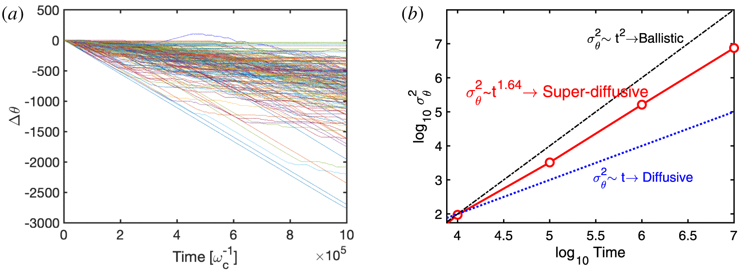
Figure 7. (a) Poloidal displacement of passive tracers showing a spreading in the poloidal direction. (b) Time dependence of the variance of the poloidal displacement.
The existence of anomalous diffusion implies that the motion of the guiding centres cannot be modelled using a diffusion equation, which has important consequences when trying to predict the transport of energetic particles by means of reduced fluid models. As explained in del-Castillo-Negrete (Reference del-Castillo-Negrete1998), the anomalous diffusion is understood as follows (Lesieur Reference Lesieur2008). Let us consider the Lagrangian velocity
 $$\begin{eqnarray}\frac{\text{d}\unicode[STIX]{x0394}\unicode[STIX]{x1D703}}{\text{d}t}=v^{\unicode[STIX]{x1D703}}(t)\end{eqnarray}$$
and the Lagrangian diffusion coefficient
 $$\begin{eqnarray}{\mathcal{K}}(t)=\frac{1}{2}\frac{\text{d}}{\text{d}t}\left\langle \left(\unicode[STIX]{x0394}\unicode[STIX]{x1D703}-\langle \unicode[STIX]{x0394}\unicode[STIX]{x1D703}\rangle \right)^{2}\right\rangle ,\end{eqnarray}$$
 which can simply be expressed as  ${\mathcal{K}}(t)=\int _{0}^{t}\langle v^{\unicode[STIX]{x1D703}}(\unicode[STIX]{x1D70F})v^{\unicode[STIX]{x1D703}}(0)\rangle \,\text{d}\unicode[STIX]{x1D70F}=\int _{0}^{t}{\mathcal{C}}(\unicode[STIX]{x1D70F})\,\text{d}\unicode[STIX]{x1D70F}$. Therefore, the time derivative of the variance is expressed in terms of the integral of the Lagrangian velocity auto-correlation function as follows
 $$\begin{eqnarray}\frac{\text{d}\unicode[STIX]{x1D70E}_{\unicode[STIX]{x1D703}}^{2}}{\text{d}t}=2\int _{0}^{t}{\mathcal{C}}(\unicode[STIX]{x1D70F})\,\text{d}\unicode[STIX]{x1D70F}.\end{eqnarray}$$
 Therefore, the scaling of the variance depends on how the Lagrangian velocity auto-correlation function decays in time. If the auto-correlation function decays fast enough in time, the integral (4.5) exists in the limit  $t\rightarrow \infty$, meaning that $\unicode[STIX]{x1D70E}_{\unicode[STIX]{x1D703}}^{2}\sim t$ and defining the diffusion coefficient ${\mathcal{K}}$. If the auto-correlation function exhibits an algebraic decay (for $\unicode[STIX]{x1D6FE}\neq 1$) as ${\mathcal{C}}\sim t^{\unicode[STIX]{x1D6FE}-2}$, then $\unicode[STIX]{x1D70E}_{\unicode[STIX]{x1D703}}^{2}\sim t^{\unicode[STIX]{x1D6FE}}$. The anomalous diffusion is therefore related to the slow decay of the auto-correlation function. This behaviour is understood in terms of the physics at play. Indeed, an energetic counter-passing particle is injected in the inner region of the tokamak and will remain rotating in the clockwise direction unless something (the chaotic separatrix) makes it change its radial position until it becomes magnetically trapped. Once it is trapped, the poloidal displacement vanishes on average (there is no transport). The particle will remain trapped unless the chaotic separatrix makes it change again its radial position. It will become either co-passing, evolving as if the particle was flying towards positive poloidal angles, or counter-passing, evolving as if the particle was flying towards negative poloidal angles. A super-diffusion can therefore be understood as a compromise between trapping periods and short and rare events called flights, which tend to de-trapped the particles. More specifically, we interpret the observed super-diffusive transport in the framework of the continuous time random walk (CTRW) model. The CTRW extends the standard Brownian random walk (which underlies diffusive transport) by allowing non-Gaussian jump distributions and/or non-Markovian waiting time distributions (Montroll & Weiss Reference Montroll and Weiss1965; Metzler & Klafter Reference Metzler and Klafter2000), caused by the presence of coherent structures (magnetically trapped and passing regions) which make particles spend an anomalous amount of time moving slowly (trapping region) or fast (passing region) (del-Castillo-Negrete Reference del-Castillo-Negrete1998), the bridge between both being ensured by the chaotic separatrix. Of particular interest to this work is the case of Lévy flights which are jumps with diverging second moments.
The existence of the flights is clearly visible in figure 8(a), where we plot the poloidal displacement of two tracers during the first  $10^{6}$ cyclotron periods. It can be observed that sometimes the particle is magnetically trapped and therefore the poloidal displacement does not evolve on average. Sometimes, the particles are de-trapped and exhibit either positive or negative flights. As a comparison, we give in figure 8(b) a time trace assuming an asymmetric standard random walk, in the absence of any flights.

Figure 8. (a) Poloidal displacement of two passive tracers, showing the existence of positive and negative flights. (b) Poloidal displacement assuming an asymmetric random walk.
Coming back to figure 6, when an EP becomes trapped it is lost if the wall of the tokamak intercepts the chaotic region, which is the case here since  $a=150\unicode[STIX]{x1D70C}_{\text{th}}$. The exit time of a counter-passing particle is related to the time a particle spends moving towards negative poloidal angles, since the particle remains in the inner region of the tokamak. Accordingly, the probability distribution function of the exit time, ${\mathcal{P}}_{\text{exit}}$, corresponds to the PDF of the negative flights of duration $t$,
$t$,  ${\mathcal{P}}_{\text{flight}}^{-}$, i.e.
 $$\begin{eqnarray}{\mathcal{P}}_{\text{exit}}\equiv {\mathcal{P}}(t_{\text{exit}}=t)={\mathcal{P}}_{\text{flight}}^{-}(t).\end{eqnarray}$$
Figure 9. PDF of negative (a) and positive (b) flight events of duration  $t$.
$t$.
To verify this connection, figure 9 shows the probability distribution function of negative (a) and positive (b) flights of duration  $t$. As expected, the PDF of negative flights exhibits an algebraic decay, ${\mathcal{P}}_{\text{flight}}^{-}\sim t^{-\unicode[STIX]{x1D707}_{f}}$, with $\unicode[STIX]{x1D707}_{f}\approx \unicode[STIX]{x1D707}_{e}$, where as shown in figure 4 ${\mathcal{P}}_{\text{exit}}\sim t^{-\unicode[STIX]{x1D707}_{e}}$. The PDF of positive flights decays faster, following an exponential scaling ( ${\mathcal{P}}_{\text{flight}}^{+}\sim \text{e}^{-\unicode[STIX]{x1D706}t}$). This finding has a physical impact in terms of radial transport: a counter-passing particle spends, probabilistically speaking, more time in the inner region than a co-passing particle in the outer region. This leads to an asymmetrically poloidal (and therefore radial) transport in the presence of the chaotic separatrix. Note that, because $\unicode[STIX]{x1D707}_{f}<3$, the second moment of the PDF of negative flights diverges, $\int _{0}^{\infty }t^{2}{\mathcal{P}}_{\text{flight}}^{-}\,\text{d}t\rightarrow \infty$. That is, the negative flights are Lévy flights which invalidates the use of the central limit theorem (CLT) as it is customary done in the Brownian random walk model of diffusive transport. On the other hand, within the CTRW, superdiffusive behaviour, $\unicode[STIX]{x1D6FE}>1$, is a natural consequence of the existence of Lévy flights, $\unicode[STIX]{x1D707}_{f}<3$. In particular, according to CTRW theory $\unicode[STIX]{x1D6FE}=2/(\unicode[STIX]{x1D707}_{f}-1)$ which for the numerically determined exponent $\unicode[STIX]{x1D707}_{f}\approx 2.2$ predicts $\unicode[STIX]{x1D6FE}=1.66$, a value very close to the numerically observed $\unicode[STIX]{x1D6FE}\approx 1.64$. Let us remember that the theory of the Brownian motion relies upon the application of the CLT, which states that the sum of $N$ independent and identically distributed (i.i.d.) random variables $\{{x_{i}\}}_{1\leqslant i\leqslant N}$ is described by a Gaussian distribution in the limit $N\rightarrow \infty$, as long as the first and second moments exist, i.e. $\langle x_{i}\rangle <\infty$ and $\langle x_{i}^{2}\rangle <\infty$. One can naturally ask what happens in the case where one of the moments (or even both) does not exist, which is our case. Fortunately, there is a generalisation of the CLT for this kind of situations, which was formulated by P. Lévy in the 1930s. The Gaussian distribution function as limit of the sum of i.i.d. variables is replaced by the so-called Lévy or $\unicode[STIX]{x1D6FC}$-stable distribution, characterised by long heavy tails and diverging moments (see for instance Lévy (Reference Lévy1934, Reference Lévy1940) and references therein).
Back to our physical problem, figure 10 shows the PDF of the total (summed) poloidal displacements at different times as a function of the similarity variable
 $$\begin{eqnarray}\unicode[STIX]{x1D712}=\frac{\unicode[STIX]{x0394}\unicode[STIX]{x1D703}-\langle \unicode[STIX]{x0394}\unicode[STIX]{x1D703}\rangle }{t^{\unicode[STIX]{x1D6FE}/2}}.\end{eqnarray}$$
 The definition of this variable is not a coincidence. Indeed, the collapse of the rescaled PDFs at different times provides numerical evidence that poloidal transport exhibits self-similar dynamics with anomalous exponent  $\unicode[STIX]{x1D6FE}$ which, consistent with the CTRW model, is equal to the numerically determined super-diffusive exponent $\unicode[STIX]{x1D6FE}\approx 1.64$. Formally, the observed self-similar evolution implies the existence of a scaling function $F$ satisfying ${\mathcal{P}}_{\unicode[STIX]{x0394}\unicode[STIX]{x1D703}}=t^{-\unicode[STIX]{x1D6FE}/2}F(\unicode[STIX]{x1D712})$.
It is observed that the scaling function departs significantly from a Gaussian distribution (represented by a dashed grey line for comparison, which is representative of diffusive processes). Also, the asymmetry in the flights is reflected in the asymmetry of the scaling function. Moreover, according to the CTRW, it should exhibit an algebraic decay of the  $\unicode[STIX]{x1D712}<0$ tail of the form $F\sim \unicode[STIX]{x1D712}^{-(\unicode[STIX]{x1D6FC}^{-}+1)}$ with $\unicode[STIX]{x1D6FC}^{-}=\unicode[STIX]{x1D707}_{f}-1$, a result fully consistent with the numerically obtained values $\unicode[STIX]{x1D707}_{f}\approx 2.2$ and $\unicode[STIX]{x1D6FC}^{-}\approx 1.2$. For the $\unicode[STIX]{x1D712}>0$ tail, within the CTRW, the exponential decay of ${\mathcal{P}}_{\text{flight}}^{+}$ implies, consistent with the numerical results, $\unicode[STIX]{x1D6FC}^{+}>2$. This is represented in the insets of figure 10 showing the log–log plots of the tails of the PDF.

Figure 10. Rescaled PDF of poloidal displacements at different times:  $\unicode[STIX]{x1D714}_{c}t=9\times 10^{6}$ (dashed magenta), $\unicode[STIX]{x1D714}_{c}t=9.5\times 10^{6}$ (dotted red) and $\unicode[STIX]{x1D714}_{c}t=10^{7}$ (solid black). The dotted-dashed grey line corresponds to a Gaussian PDF. The insets represent the log–log plots of the tails, showing the asymmetric algebraic decays.
5 Conclusions and future work
In this paper, we have explored the fundamental mechanism of the transport of energetic particles (EP) in the presence of an oscillating radial electric field in axisymmetric tokamak magnetic equilibria. Such scenarios can be found in the presence of EGAMs, as reported for instance in Fisher et al. (Reference Fisher, Pace, Kramer, Van Zeeland, Nazikian, Heidbrink and García-Muñoz2012), Nazikian et al. (Reference Nazikian, Fu, Austin, Berk, Budny, Gorelenkov, Heidbrink, Holcomb, Kramer and McKee2008) and Zarzoso et al. (Reference Zarzoso, del-Castillo-Negrete, Escande, Sarazin, Garbet, Grandgirard, Passeron, Latu and Benkadda2018). We show in particular that initially integrable orbits are transformed into chaotic regions that can intercept the wall of the tokamak, leading to losses of EP. We have provided numerical evidence of fractal-like patterns and anomalous exit time statistics of EP, exhibiting algebraic decay in sharp contrast with the expected exponential exit time in the case of radial diffusive transport. We have shown that the algebraic loss time decay is the result of Lévy flights that lead to super-diffusive poloidal transport and an asymmetric non-Gaussian (Lévy) PDF of displacements. Since the radial displacement is related to the sign of the time derivative of the poloidal angle, the observed poloidal displacement asymmetry translates into a radial displacement asymmetry and EP can spend probabilistically speaking more time in the inner region of the tokamak than in the outer one. These results might have an important impact on the confinement time of EP needed to achieve sustained fusion in burning plasmas, in addition to the potential generation of a toroidal net torque resulting from the poloidal asymmetry of the particle displacements.
The work presented in this paper opens the doors to further analyses that have not been addressed here. First, the observed anomalous radial transport should be quantified in the presence of other mechanisms that could be responsible of diffusive transport. Second, the dependence of the transport (diffusive, super- or sub-diffusive) on the parameters characterising the oscillating radial electric field should be studied in detail. Third, quantifying the generation of momentum due to the radial asymmetric displacement is essential in order to assess its effect in future plasma scenarios. Finally, it is known that fractional diffusion results from the continuum (fluid) limit of the (kinetic) CTRW model, see e.g. del-Castillo-Negrete, Carreras & Lynch (Reference del-Castillo-Negrete, Carreras and Lynch2004) and Metzler & Klafter (Reference Metzler and Klafter2000). Accordingly, the observed self-similar dynamics of the PDF of poloidal displacements, along with the consistency of the numerically determined anomalous exponents  $\unicode[STIX]{x1D707}_{e}$, $\unicode[STIX]{x1D6FE}$, $\unicode[STIX]{x1D707}_{f}$, $\unicode[STIX]{x1D6FC}^{-}$ and $\unicode[STIX]{x1D6FC}^{+}$ with the CTRW predictions, opens the possibility to describe EP transport using non-local transport models based on fractional derivatives (del-Castillo-Negrete Reference del-Castillo-Negrete2006). These four directions of research will be explored in a forthcoming publication.
Acknowledgements
D.d.-C.-N. was sponsored by the Oak Ridge National Laboratory, managed by UT-Battelle, LLC, for the US Department of Energy under Contract no. DE-AC05-00OR22725.


