


1. INTRODUCTION
Positioning technologies have become increasingly important in our daily lives. Global Navigation Satellite Systems (GNSS) can provide 24/7 high accuracy positioning, navigation and timing (PNT) services to most outdoor applications such as surveying and geodesy, car and personal navigation, airborne mapping and sensor geo-referencing, and many others. In addition to the conventional outdoor location based service (LBS), there are many needs for indoor positioning, for example, warehouse logistics management, fire fighting and emergency services, underground construction, etc. All these applications require comparatively high accuracy but are beyond current GNSS positioning capability because GNSS signals are generally unavailable in many indoor environments. Alternatives to GNSS are the many radio-frequency approaches that have been developed over the past decades, including Bluetooth (Altini et al., Reference Altini, Brunelli, Farella and Benini2010; Fischer et al., Reference Fischer, Dietrich and Winkler2004), Radio Frequency Identification (RFID) (Chumkamon et al., Reference Chumkamon, Tuvaphanthaphiphat and Keeratiwintakorn2008), Ultra Wideband (UWB) (Gigl et al., Reference Gigl, Janssen, Dizdarevic, Witrisal and Irahhauten2007), Wireless Local Area Net (WLAN) and pseudolites. In addition, self-contained inertial navigation technology is widely used for indoor pedestrian navigation. Table 1 compares some key indoor technologies in terms of their typical accuracy and coverage (Mautz, Reference Mautz2012). It can be seen from the table that, of all techniques considered, pseudolites can achieve the highest accuracy of centimetre to decimetre level. However, there are some problems that limit the applicability of pseudolites.
Table 1. Overview of indoor positioning technology.

The first one is the synchronisation of pseudolite transmitters (Kanli, Reference Kanli2004; Driscoll et al., Reference Driscoll, Borio and Fortuny2011; Barnes et al., Reference Barnes, Wang, Rizos and Tsujii2002). Most pseudolites operate unsynchronised or synchronised to each other by sharing a common clock and being connected with cables of the same length, or by setting up a nearby base station (an additional receiver) to mitigate the pseudolite clock errors using differential positioning techniques (as in GNSS). However, both methods are costly and not realistic for many applications. The second problem is the so-called “near-far problem” (Cobb, Reference Cobb1997; Kanli, Reference Kanli2004). The range of Analogue to Digital (A/D) converters used for the receiver is small which makes it difficult for the receiver to detect strong and weak signals at the same time. For example, if a receiver is very close to a transmitter its received signal will be so strong that it could jam the relatively weak signals from the more distant transmitters because the transmission power is inversely proportional to the square of the distance. The third problem is the multipath disturbance effect. Because of the walls and many reflecting objects, the receiver may receive the signal from more than one path, which can cause deep fading and pulse spreading of the signal (Tam and Tran, Reference Tam and Tran1995). The multipath effect for all terrestrial-based PNT systems is very challenging.
The Locata technology is a terrestrial-based system, which uses a “local constellation” of ranging signals operating under local control to address local user requirements. A number of papers have been published on Locata technology for both indoor and outdoor applications (Barnes et al., Reference Barnes, Rizos, Wang, Meng, Dodson and Roberts2003, Reference Barnes, Rizos and Kanli2004; Choudhury et al., Reference Choudhury, Rizos and Harvey2009a; Li and Rizos, Reference Li and Rizos2010; Montillet et al., Reference Montillet, Roberts, Hancock, Meng, Ogundipe and Barnes2009; Rizos et al., Reference Rizos, Roberts, Barnes and Gambale2010). Locata originated from the pseudolite concept, but differs from conventional pseudolites in some important ways. Locata deals with the synchronisation problem using a technique known as the “TimeLoc” process. By doing this, the time difference can achieve a few nanoseconds and the frequency stability is less than one part per billion (ppb) (Gauthier et al., Reference Gauthier, Glennon, Rizos and Dempster2013). With synchronised transmission, a pulsing pattern can be used to deal with the near-far effect. The typically used multipath-mitigating approach of “elevation masking” is not suitable since there are more reflective surfaces and many of them tend to be perpendicular to the signal path. Several techniques have been implemented in radio systems to minimise multipath, including correlation techniques and radio-frequency techniques (Kim et al., Reference Kim, De Lorenzo, Akos, Gauter, Enge and Orr2004). However these techniques are primarily used for anti-jam applications and are not effective against multipath because of the relatively wide signal beamwidth. In this paper, a new multi-beam antenna – the Locata “V-Ray” designed to mitigate multipath effects by use of sufficiently tight beams – is described in Section 2.
The receiver sweeps the beams and searches for the optimal beam settings that point directly to the Locata transmitters. Direct line-of-sight pseudorange and carrier phase measurements can then be obtained. In addition to the standard range measurements, the V-Ray antenna can be used to determine the body frame attitude using angle-of-arrival measurements (LaMance and Small, Reference LaMance and Small2011). The V-Ray antenna has a spherical shape, and hence the formed beams can be pointed in any direction and used to determine 3D attitude with a single antenna. Attitude determination based on these unique Locata angle-of-arrival measurements is described in Section 3.
The conventional method for attitude determination using GNSS is to set up three or more receivers/antennas mounted on the platform and determine the relative position from differenced carrier phase measurements (Cohen, Reference Cohen, Parkinson and Spilker1996). However, this method requires simultaneous observations from all the receivers. In this paper, a position and attitude modelling system (PAMS) is proposed for the determination of position, velocity and platform attitude using a single Locata receiver/antenna.
The range and angle measurements are processed simultaneously by one system filter. Unlike conventional attitude determination using gyroscopes, PAMS does not need to deal with time-dependent drift errors. Since both the range measurement model and the angle measurement model are non-linear, the Unscented Kalman Filter (UKF) is adopted. A short description of the UKF and details of the PAMS are presented in Section 4.
The PAMS is evaluated in a field test conducted in a metal warehouse in which the multipath effects are severe. The experiment is described, and analyses are presented, in Section 5.
2. LOCATA TECHNOLOGY AND V-RAY ANTENNA
Locata is the technology derived from the pseudolite concept, though there are some significant differences with respect to conventional pseudolites. The key problems with pseudolites are the so-called “near-far” effect and signal transmitter synchronisation. The conventional solutions to these problems are random pulsing for the former, and use of differential reference stations for the latter (Cheong et al., Reference Cheong, Dempster and Rizos2009). Locata deals with the synchronisation problem using a technique known as “TimeLoc” which permits the synchronisation of the “LocataLite” transmitters to nanosecond-level for time difference and less than one ppb for frequency stability. With synchronised transmission, a pulsing pattern to deal with the near-far effect can be used (Locata, 2011).
Locata transmits signals from two separate antennas to provide “spatial diversity”. Each antenna transmits two signals approximately 60 MHz apart to ensure “frequency diversity” (2·41428 GHz and 2·46543 GHz – referred to as S1 and S6 respectively). As a result there are four independent signals transmitted by each LocataLite.
Locata uses signals chipped at 10·23 MHz, which reduces the chip distance to about 30 metres and makes it easier to eliminate the long-wave multipath that causes more than two chips delay. However, in indoor environments, the challenging problem for Locata receivers is short-wave multipath causing delays of less than one chip.
An effective way to reduce the multipath disturbance of the transmitted signal is by pointing a narrow beam antenna in the known signal direction, which inhibits the reception of signals from all but the desired direction. With a sufficiently narrow beam, the multipath corrupted signals can be removed at the user receiver. However, narrow beams are hard to generate, and would ordinarily require a large number of antenna elements. The typical beam-forming antennas use multiple RF front-ends to form tight beams, however the cost and phase-based positioning precision degradation limits the usefulness of such beam-forming antennas.
Locata's new beam-forming method is known as Correlator Beam-Forming (CBF). This method creates beams by sequentially switching through each element of an antenna array and forming the beam with phase and gain corrections in the receiver's individual channel correlators, using only one RF front-end. CBF gives each receiver channel the capability to independently “point” beams. The V-Ray antenna is capable of pointing multiple beams simultaneously in different directions. The elements are sequentially switched, and the elements are sequenced completely during a signal integration interval. During each switch interval, the gain and phase of the incoming signal is adjusted within the correlator by modifying the phase and amplitude of the carrier DCO to form the desired beam. The process is illustrated in Figure 1 (LaMance and Small, Reference LaMance and Small2011).

Figure 1. Locata V-Ray principle (LaMance and Small, Reference LaMance and Small2011).
To mitigate multipath, the beams must be pointed in the directions of the LocataLites. The position of each LocataLite is known, thus each beam's direction is dependent on the location of the rover and the orientation of the antenna. Both rough position and orientation are estimated from angle-of-arrival measurements by analysing the signals obtained from different beam settings. The receiver sweeps the beams searching for beam settings that maximise the signal from each LocataLite. Once the optimal beam settings are determined, the corresponding angle-of-arrival measurements are used to estimate both the approximate location of the rover and the orientation.
The current “V-Ray” antenna is a basketball-sized spherical array consisting of 20 panels with 80 elements. Each panel comprises four elements arranged with one central element and the three other elements forming a triangle. The element spacing between each panel is half the signal wavelength (LaMance and Small, Reference LaMance and Small2011). The V-Ray beam-forming antenna is shown in Figure 2.
Figure 2. Locata beam forming V-Ray antenna.
V-Ray needs only one RF front-end for all elements, which is a simple and non-expensive antenna design. Every beam is controlled individually, hence as the platform on which the antenna is mounted moves, each beam adjusts dynamically. The elements are switched through at a rate of 80 elements every 100 microseconds, and more than 2·5 million individual steered beams per second can be produced. The switches are implemented by a simple Programmable Logic Device (PLD), and the timing for the PLD switch control is provided by the digital section of the receiver.
With its spherical shape the V-Ray antenna has the ability to point in any direction (3D). The new generation Locata receiver is designed to deal with hundreds of simultaneous, unique beams every 100 microseconds, and hence can make measurements from many directions at once. However, the Locata receiver used in this experiment had experimental firmware that only enabled it to process thousands of beams per second. Therefore only the azimuth measurements could be decoded to obtain one-axial orientation solutions.
3. LOCATA POSITION AND ATTITUDE COMPUTATION MODEL
3.1. Locata positioning measurement model
Similar to GNSS, the Locata range measurements are of two types: pseudorange and carrier phase. The carrier phase measurements are more precise than the pseudorange measurements, and the basic carrier phase observation equation associated with a receiver and LocataLite channel i can be written as:
 $$\phi ^i \cdot \lambda = \rho ^i + \tau _{trop}^i + c \cdot \delta T + N^i \cdot \lambda + \varepsilon _\phi ^i $$
where ϕi is the carrier phase measurement (in cycles); ρi is the geometric range from receiver to the transmitting antenna i; λ is the wavelength of the carrier signal; τ tropi is the tropospheric delay; c is the speed of Electromagnetic Radiation (EMR); δT is the receiver clock bias; Ni is the carrier phase ambiguity, and ε ϕi is the lumped sum of un-modelled residual errors (including noise). Note that there is no transmitter clock error in the observation equation because of the tight time synchronisation of the LocataLites. Nor is there an ionospheric delay term.
The receiver clock error may be estimated, or eliminated using measurement differencing. To eliminate the receiver clock the carrier phase measurements of the same frequency are Single-Differenced (SD). The tropospheric delays in Δτ tropij must be calculated using an appropriate tropospheric model (Choudhury et al., Reference Choudhury, Harvey and Rizos2009b). When j is chosen as the reference signal, and i is another signal of the same frequency, the SD Δϕij is:
 $$\Delta \phi ^{ij} \cdot \lambda = (\phi ^i - \phi ^j ) \cdot \lambda = \Delta \rho ^{ij} + \Delta \tau _{trop}^{ij} + N^{ij} \cdot \lambda + v$$
The unknown parameters are the receiver's coordinates (x R, yR, zR) in the SD geometric range Δρij. Locata carrier ambiguities Nij are also unknown parameters that could be determined in pre-processing by the method of “known point initialization” (KPI), which is based on the following relation:
 $$\Delta N^{ij} \cdot \lambda = \Delta \phi _0^{ij} \cdot \lambda - \Delta \rho _0^{ij} - \Delta \tau _{trop}^{ij} - v$$
To calculate precise Δρ 0ij, the initial position of the Locata rover needs to be surveyed precisely. Standard survey techniques (Total Station, or a survey-grade GNSS if outside) can be used to obtain the initial coordinates. Once the floating ambiguities are estimated, they can be treated as “fixed” (known) parameters in (2).
3.2. Locata angle computation model
V-Ray is a 3D antenna which can in principle measure attitude angles in three orthogonal directions. However, the firmware version that was available for these tests only allowed the measurement of azimuth. The azimuth angle measurement is the angle between the signal source (the LocataLite) and the reference direction on the receiver's body frame, see Figure 3, where ψ is the orientation angle of the platform and α is the measured azimuth angle.
Figure 3. Locata angle measurement.
The angle measurement function can be written as:
 $$\alpha + \psi = \arctan \left( {\displaystyle{{x_{LL} - x_R} \over {y_{LL} - y_R}}} \right)$$
where x LL and y LL are the horizontal coordinates of the LocataLites in the local reference frame, and x R and y R are the horizontal coordinates of the receiver in the same frame.
4. PAMS MECHANIZATION
4.1. UKF introduction
The Extended Kalman filter (EKF) is a commonly used estimator for non-linear navigation systems, however it has several drawbacks due to the linearization scheme that is employed. In the EKF, the state distribution is propagated through the first-order linearization of the non-linear system (using the Jacobian matrix). This process will introduce large errors in the true posteriori mean and covariance of the transformed variables, which leads to sub-optimal performance, and sometimes filter divergence (Wan and Van der Merwe, Reference Wan and Van der Merwe2000). To overcome this shortcoming the Unscented Kalman Filter (UKF) has been developed using a deterministic sampling approach (Julier et al., Reference Julier, Uhlmann and Durrant-Whyte1995). The basic premise of the UKF is that it is easier to approximate a probability distribution than an arbitrary non-linear function. The state distribution is represented by a set of selected sample points that capture the mean and covariance information. The sample points are directly propagated through the true non-linear function, and hence the linearization of the model is avoided (Zhang et al., Reference Zhang, Gu, Milios and Huynh2005). The posteriori mean and covariance can be represented accurately to the third-order of Taylor series expansion of the non-linear function, and hence has an obvious advantage over the EKF.
4.1. PAMS estimation process
From the Locata V-Ray antenna, the multipath-mitigated pseudorange, carrier phase and angle (azimuth) measurements are available. The PAMS system is designed with a common filter to process range and azimuth measurements simultaneously, and outputs the full set of navigation parameters (position, velocity, acceleration and attitude).
4.1.1. Dynamic model
A benefit of a KF compared with the conventional least–squares method is the KF's utilisation of a dynamic model for the rover. The state vector of the system consists of ten parameters (three for position, three for velocity, three for acceleration and one orientation angle). Typically the acceleration is modelled as a white noise process. (A white noise process is “isolated” in time since its value at one epoch is uncorrelated with the values at any other epoch.) However, the acceleration of the host platform is dominated by the thrust, which has a strong temporal correlation. In such a case it is appropriate to model the acceleration as a first-order Gauss Markov process rather than as a white noise process. The acceleration model is:
 $$\dot a = - (1/\tau ) \cdot a + \omega _a $$
with associated dynamic driving noise process given by:
 $$E{\rm \{} \omega _a (t)\omega _a (t + T){\rm \}} = \displaystyle{{2\sigma ^2} \over \tau} \delta (T)$$
where τ is the correlation time constant; and σ 2 is the acceleration variance, with τ=3600 s and σ=0·25 m/s 2 selected in this filter. The position and velocity states do not include any direct driving noise, and their estimation relies entirely on the other states and the actual measurements.
The system state can be represented as:
 $${\bf x}(t) = [\matrix{ {\bf r} & {{\bf \dot r}} & {{\bf \ddot r}} & \psi \cr} ]^{\rm T} $$
where r,  ${\bf \dot r}$ and ${\bf \ddot r}$ are platform position, velocity and acceleration vectors (in three dimensions) respectively.
The dynamic model is:
 $${\bf \dot x}(t) = {\bf F}(t) \cdot {\bf x}(t) + {\bf \omega} (t)$$
where 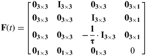 ${\bf F}(t) =\hskip-2pt \left[ {\matrix{ {{\bf 0}_{{\bf 3} \times {\bf 3}}} & {{\bf I}_{{\bf 3} \times {\bf 3}}} & {{\bf 0}_{{\bf 3} \times {\bf 3}}} & {{\bf 0}_{{\bf 3} \times {\bf 1}}} \cr {{\bf 0}_{{\bf 3} \times {\bf 3}}} & {{\bf 0}_{{\bf 3} \times {\bf 3}}} & {{\bf I}_{{\bf 3} \times {\bf 3}}} & {{\bf 0}_{{\bf 3} \times {\bf 1}}} \cr {{\bf 0}_{{\bf 3} \times {\bf 3}}} & {{\bf 0}_{{\bf 3} \times {\bf 3}}} & { - \displaystyle{{\bf 1} \over {\bf \tau}} \cdot {\bf I}_{{\bf 3} \times {\bf 3}}} & {{\bf 0}_{{\bf 3} \times {\bf 1}}} \cr {{\bf 0}_{{\bf 1} \times {\bf 3}}} & {{\bf 0}_{{\bf 1} \times {\bf 3}}} & {{\bf 0}_{{\bf 1} \times {\bf 3}}} & 0 \cr}} \right]\hskip-4pt $, ${\bf \omega} (t) = [\matrix{ {{\bf 0}_{{\bf 1} \times {\bf 3}}} & {{\bf 0}_{{\bf 1} \times {\bf 3}}} & \hskip-2pt{\omega _a} & \hskip-2pt{\omega _a} & \hskip-2pt {\omega _a} & \hskip-2pt {\omega _\psi } \cr} ]^{\rm T} , $ the orientation angle is modelled as white noise, implying $\dot \psi = \omega _\psi $.
4.1.2. Measurement model
The carrier phase and azimuth measurement Equations (2) and (4) are both non-linear, thus the PAMS measurement model is non-linear. The measurement model of the Locata filter is:
 $${\bf z}(t) = {\bf h}({\bf x}(t)) + {\bf \upsilon} (t)$$
where z(t) is the measurement vector of the filter, which is formed by the SD carrier phase measurements and azimuth measurements:
 $${\bf z}({\bf t}) = \left[ {\matrix{ {{\bf\Delta \varphi} _{{\bf 1} \times {\bf m}}} & {{\bf \alpha} _{{\bf 1} \times \left( {{\bf m} + {\bf 2}} \right)}} \cr}} \right]^{\rm T} = \left[ {\matrix{ {\Delta \phi ^{1j}} & {\Delta \phi ^{2j}} & \cdots & {\Delta \phi ^{mj}} & {\alpha ^1} & {\alpha ^2} & \cdots & {\alpha ^{m + 2}} \cr}} \right]^{\rm T} $$
where m is the number of SD carrier phase measurements. Since the Locata signals are transmitted on two frequencies and the azimuth measurements are not single-differenced, the number of azimuth measurements is m+2.
h(x(t)) is the non-linear transformation function, which can be represented as:
 $${\bf h}({\bf x}(t)) = [\matrix{ {{\bf h}_\phi ({\bf x}(t))} & {{\bf h}_\alpha ({\bf x}(t))} \cr} ]^{\rm T} $$
where hϕ(x(t)) and hα(x(t)) are derived from the carrier phase and azimuth measurement functions in Equations (2) and (4). υ(t)~N(0, R) is the measurement noise. The R matrix consists of SD carrier phase and azimuth components, given by:
 $${\bf R} = \left[ {\matrix{ {{\bf R}_{\Delta \phi}} & {} \cr {} & {{\bf R}_\alpha} \cr}} \right]$$
Since SD carrier phase measurements are correlated with each other, the covariance is therefore assumed to be half of the variance:
 $${\bf R}_{\Delta \phi} = \displaystyle{{\sigma _{\Delta \phi} ^2} \over 2}\left[ {\matrix{ 2 & 1 & \cdots & 1 \cr 1 & 2 & \cdots & 1 \cr \vdots & \vdots & \ddots & 1 \cr 1 & 1 & 1 & 2 \cr}} \right]$$
The azimuth measurement covariance sub-matrix can be written as:
 $${\bf R}_\alpha = \sigma _\alpha ^2 \cdot {\bf I}_{(m + 2) \times (m + 2)} $$
where σ Δϕ2 and σ α2 are the noise variance of the SD carrier phase measurements and azimuth measurements, respectively.
5. EXPERIMENT AND ANALYSES
The indoor experiment was conducted in a metal building at Locata Corporation's Numerella Test Facility (NTF), located in rural NSW, Australia. The warehouse was mostly empty with the exception of some furniture and tools placed near the walls. Five LocataLites were installed in the corners of the warehouse. Table 2 shows the coordinates of the five LocataLites in latitude (degree), longitude (degree) and height (metre). A Locata rover receiver was placed on a trolley with the V-Ray antenna mounted on it. Figure 4 shows the testing environment. The benchmark system was an auto-tracking Total Station (TS), which could provide position and orientation and attitude information. The orientation of the antenna from the TS was determined by measuring the two prisms on the bar as shown in Figure 4.
Figure 4. Indoor testing environment at NTF’.
Table 2. Configuration of LocataLites.

It can be seen from Table 2 that the LocataNet was configured in an almost planar configuration and the line-of-sight between the rover and the LocataLites is also mainly planar, thus the vertical geometry is not good enough for height measuring. For that reason a pre-measured distance between the antenna and the ground is used to constrain the height solutions. The rover trajectory is shown in Figure 5 as the blue line, while the red dots and blue dots represent the static points and the locations of the LocataLites, respectively. The test started from Point 1. The rover stayed at Point 1 at the beginning and then moved sequentially to each other point, stopping for several minutes. There were 21 static points in total.
Figure 5. Rover trajectory and LocataLite installation.
The system first solved for the float-value ambiguities using the KPI method, and then the UKF estimation provided the position and attitude estimates. The TS measured the “true” values at the 21 static points.
Figure 6 is the scatter diagram of the position differences (compared to the truth solutions from the TS) for the horizontal direction components. The red dot indicates the origin of the coordinate system. The outer circle has a radius of 4 cm and the inner circle a radius of 2 cm. It can be seen that most points are located inside the 4 cm radius circle.
Figure 6. Performance at all 21 individual test points.
Further analysis of the mean values and standard deviations (STD) of the north and east position components are shown in Figures 7 and 8. The 21 bar charts in each plot represent the data calculated at the 21 static points. It can be seen that in all cases the positioning accuracy is at the centimetre-level. The STD value indicates that the solution is very stable. The root mean square (RMS) of the whole trajectory was 0·017 m for the north component and 0·018 m for the east component.
Figure 7. Mean and STD of the position difference in the north component.
Figure 8. Mean and STD of the position difference in the east component.
The 2D RMS was calculated and plotted in Figure 9. The 2D RMS of the whole trajectory was 0·025 m, and the 2D RMS for all 21 points was less than 4 cm, which confirms that the Locata PAMS system in an indoor environment can achieve stable and accurate horizontal solutions.
Figure 9. 2D RMS evaluation of horizontal positioning.
As discussed in Section 3, both Locata range and azimuth measurement functions are non-linear, thus the UKF was implemented in the PAMS instead of the commonly used EKF. A comparison of the horizontal positioning performance of the UKF and EKF is shown in Figures 10 and 11, where the blue line and the red line denote the position differences in EKF and UKF systems, respectively. Apart from the system estimation filter, all other stochastic conditions were the same. In order to more clearly indicate the differences, the plots in Figures 10 and 11 are a segment of the whole trajectory (one of the 21 static points). It can be seen that basic positioning error trends of the two systems are the same, however the UKF system has a slightly better accuracy for both the north and east components. The corresponding RMS comparison is given in Table 3. The UKF has a lower RMS value for both horizontal directions: 0·018 m in the north and 0·03 m in the east. Compared with those computed by the EKF there is a minor improvement of 4·3% and 2·9% for the north and east components, respectively.
Figure 10. Comparison of north position component differences calculated using the EKF and UKF.
Figure 11. Comparison of east position component differences calculated using the EKF and UKF.
Table 3. RMS comparison of positioning differences.

Due to the new azimuth measurements available from the V-Ray antenna, the azimuth measurements can be used to estimate the orientation, as well as contributing to horizontal position determination. Figure 12 shows the HDOP of the integrated range/azimuth system compared to that of the typical range-only system configuration. The bar charts in the plot are the mean HDOP calculated at the 21 static points. The red colour and the blue colour represent the integrated system HDOPs and the range-only system HDOPs, respectively. It can be seen that the mean HDOP value of the former is around 0·5, which is much lower than for the latter case. Moreover, the two points with highest HDOP (bar 8 and bar 15) in the range-only system configuration have close to mean HDOP values when the integrated range/azimuth system is considered. This indicates that the integrated range/azimuth system is able to provide more stable and accurate positioning performance compared with a range-only system.
Figure 12. HDOP comparison between typical range-based system and the integrated range/azimuth system.
The Mean and STD values of the orientation solutions were calculated and plotted in Figure 13. It can be seen that the orientation difference (from that derived by the TS) is stable and its accuracy is better than 1°. The RMS of the orientations for the whole trajectory was computed, and found to be 0·427°.
Figure 13. Mean and STD of orientation differences (full measurements).
Although the range measurement is not a direct observation of the orientation angle, it aids estimation of the rover's position, and therefore improves the observability of the orientation. In order to analyse the range measurement's influence on the orientation solutions, Figure 14 is the plot of mean and STD values of the orientation solutions which were calculated using azimuth measurements only. This system was also estimated via the UKF, and the stochastic settings for the azimuth measurements and the orientation were kept the same as in the PAMS. Comparing Figures 13 and 14 it can be seen that the mean values of the two are similar, but in terms of the STD comparison the orientation solutions of the proposed system give a more stable STD value. The two jumps in the azimuth measurement system (bar 15 and bar 19) are substantially smaller in the proposed system. This can be attributed to the smoothing effect of adding the range measurements.
Figure 14. Mean and STD of orientation differences (azimuth measurements only).
6. CONCLUDING REMARKS
This paper presents the first results of an investigation of a new position/attitude modelling system based on an innovative correlator beam-forming antenna that can provide accurate navigation information in indoor environments in the presence of severe multipath. The proposed position and attitude modelling system (PAMS) is designed to process the carrier phase and azimuth measurements simultaneously via a UKF, to obtain the complete set of navigation parameters – position, velocity, acceleration and orientation. The indoor test was conducted in a metal warehouse subjected to considerable signal multipath disturbance. A V-Ray antenna connected to a Locata rover receiver was moved slowly around the room, visiting 21 static points. The test results confirmed that the horizontal position accuracy was better than 4 cm and the orientation accuracy was better than 1°. A comparison of system models based on the UKF and EKF was conducted, indicating that the UKF has a slight improvement over the EKF. Compared to a standard range-only-based positioning system, the HDOP values of the integrated range/azimuth system are significantly decreased. Furthermore the orientation results are more stable and reliable compared to using only an angle measurement-based orientation determination system.
ACKNOWLEGEMENTS
The first author wishes to thank the Chinese Scholarship Council (CSC) for supporting her studies at the University of New South Wales. The authors acknowledge the assistance of Mazher Choudhury (UNSW) and staff of the Locata Corporation for the indoor test. According to Locata's report, Locata's real-time solution is better than 2 cm in position and 0·5° in orientation, further questions could refer to Dr. Joel Barnes (joel.barnes@locatacorp.com).


