1. INTRODUCTION
The Global Positioning System (GPS) is being widely used in safety critical air traffic services, e.g. civil aviation. To guarantee the safety of the navigation solution for these applications, a hazard analysis is necessary, where the required performances regarding accuracy, integrity, continuity and availability are to be assessed (RTCA, 2006). The integrity for a Non-Precision Approach (NPA) is of concern here, for which Receiver Autonomous Integrity Monitoring (RAIM) is used to generate a Horizontal Protection Level (HPL) for users to be aware of the level of safety.
There are two major issues when calculating the exact HPL with given integrity risk. First, the distribution of the horizontal position error is too complex to calculate the probability of position error for real time applications. Second, the determination of the worst case is also not straightforward if we are to accommodate all possible bias values. Various methods were proposed to simplify the calculation, resulting in approximated HPLs. Two approximated distributions of the horizontal position error are used in the conventional method including the normal approximation (Lee, Reference Lee1995) and the chi-squared approximation (Ober, Reference Ober1997). The former has the disadvantage of underestimating the probability in some cases while the latter is an overestimate (Ober, Reference Ober1997). Approximations are also made on the second issue to speed up the process. Without a search for the worst case, specific formulae were given in the conventional methods (Brown and Chin, Reference Brown and Chin1998; Walter and Enge, Reference Walter and Enge1995; Brenner Reference Brenner1996). These approximations can speed up the HPL computation, but they are designed to be conservative with higher protection level than the exact value. The exact HPL value can achieve higher service availability, and therefore this is pursued by solving the two major issues.
A Monte Carlo simulation is commonly used to calculate the probability of position error, which is very time consuming. Two ways to calculate the exact position error probability have been identified to be equivalent (Johnson and Kotz, Reference Johnson and Kotz1970; Ober, Reference Ober1997; Ober, Reference Ober1998): 1) the integration of the distribution for 2D position error in a quadratic form; 2) the integration of the bivariate normal distribution over a circle. Several implementations are studied and compared in the first approach (Duchesne and Lafaye de Micheaux, Reference Duchesne and Lafaye de Micheaux2010) and the one in Imhof (Reference Imhof1961) showing reliable results is used here. A method was designed in the latter approach (DiDonato and Jarnagin, Reference DiDonato and Jarnagin1961) to speed up the calculation, which was first used in navigation integrity monitoring by Milner and Ochieng (Reference Milner and Ochieng2010). These two implementations to calculate the probability can achieve a pre-defined accuracy, and they are both referred to as the “exact distribution” in this paper.
For the second issue, an iterative search was designed in Milner and Ochieng (Reference Milner and Ochieng2011) to search the worst case bias with the maximum integrity risk. But it is observed that the iterative method is not able to control the accuracy of the results with uncertainty caused by the number of steps, and is computationally heavy with two search loops. Therefore, a new approach is proposed here to improve these two performance criteria based on the method in Jiang and Wang (Reference Jiang and Wang2014) for the Vertical Protection Level (VPL) computation. A new iterative method with one search loop is designed with results showing that it has higher computational efficiency, but the accuracy of the results is still uncertain. An optimisation method is then used to generate results within a pre-defined accuracy, and also the computation is considerably faster than the other methods.
The rest of the paper is organised as follows. The basic model and parameters that are going to be used for calculation of HPL are defined in Section 2. All current methods to calculate HPL are introduced in Section 3. The two issues in calculation of the exact HPL are studied in Section 5 with numerical results in Section 6 and conclusions in Section 7.
2. NAVIGATIONAL SYSTEM MODEL AND INTEGRITY RISK
The linearised model to relate GPS observations to the position is
 $$E\left( y \right) = Ax;\; \,D\left( y \right) = {Q_y} = {P^{ - 1}}$$
where y ∈ R m×1 is the observation vector which is assumed to be Gaussian; x ∈ R n×1 is the unknown position vector including the three dimensional position error and clock error; A ∈ R m×n is the design matrix with rank n, which is derived by the elevation angle as the transformation from the observation domain to the position domain; Q y is the covariance matrix of the observations, which is modelled to account for clock and ephemeris errors, troposphere delay, multipath and receiver noise.
The least squares estimate of x is
 $$\hat x = {\left[ {\matrix{ {{{\hat x}_E}} & {{{\hat x}_N}} & {{{\hat x}_U}} & {{{\hat x}_T}} \cr}} \right]^T} = Sy$$
where  ${\hat x_E}$,
  ${\hat x_N}$,
  ${\hat x_U}$ are the east, north and up component estimation, and
  ${\hat x_T}$ is the clock estimation; S = (A TPA)−1A TP is the solution estimation matrix with each row as
  $S = {\left[ {\matrix{{{S_E}} & {{S_N}} & {{S_U}} & {{S_T}} \cr}} \right]^T}$.
RAIM utilises redundancy in observations to do a consistency check. An alarm is sent to the cockpit if an unacceptably large position error is detected to warn the pilot that GPS should not be used for navigation. In the conventional RAIM (Brown and Chin, Reference Brown and Chin1998), a chi-squared test is used to detect the failure. A multiple hypothesis structure is used to define the test statistic, which is of normal distribution
 $$t{s_i} = \displaystyle{{e_i^T P{Q_v}Py} \over {\sqrt {e_i^T P{Q_v}P{e_i}}}} $$
where i = 1 · · · m; e i ∈ R m×1 is a zero vector with the ith element as one; Q v = Q y − A(A TPA)−1A T. Under hypothesis H i:E(ts i) = δ i, δ i is the non-centrality parameter. The probability of false alarm P fai and the probability of missed detection P mdi are defined as follows with T i as the threshold,
 $${P_{\,fai}} = P\left\{ {\left\vert {t{s_i}} \right\vert \gt {T_i}{\rm \vert}{H_0}} \right\} $$
 $${P_{mdi}} = P\left\{ {\left\vert {t{s_i}} \right\vert \lt {T_i}{\rm \vert}{H_i}} \right\} $$
 Protection level is a statistical error bound to guarantee that the probability of the position error exceeding a given bound is within the required integrity risk. If the computed protection level is larger than the given alert limit, an alert within the required TTA should be generated by the system. This is an adaptation to the definition in the standards (ICAO, 2006; RTCA, 2006). The position error is the difference between the estimated value and the real one. With an HPL of concern, the horizontal position error 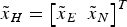 ${\tilde x_H} = {\left[ {{{\tilde x}_E}\; \; {{\tilde x}_N}} \right]^T}$ is a vector with the east position error and the north position error. Also it has been shown that the test statistic and the position error are independent (Ober, Reference Ober1997). The allocated integrity risk under H i is defined as (GEAS, 2008)
 $$I{R_i} = P\left\{ {\sqrt {\vert\vert{{\tilde x}_H}\vert{\vert^2}} \gt HP{L_i}\vert{H_i}} \right\}P\left\{ {\left\vert {t{s_i}} \right\vert \lt {T_i}{\rm \vert}{H_i}\;} \right\}{P_{{H_i}}}$$
where integrity risk IR i is a function of the probability of the horizontal position error 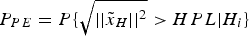 $P_{PE} = P\{ \sqrt {\vert\vert{{\tilde x}_H}\vert\vert^{2}} \gt HPL \vert H_i \}$, the prior probability of H i hypothesis
  ${P_{{H_i}}}$ and P mdi. It should be noted that the integrity risk for each hypothesis is defined to accommodate all possible bias size. In other words, Equation (6) is defined to bound the worst case bias by the given integrity risk. The worst case bias is the one that generates the biggest integrity risk. With each HPL i computed to protect the worst case bias under each hypothesis, the final HPL is the maximum one among all hypotheses with i = 0, 1 · · · m.
The risk for each hypothesis is set as (Brenner, Reference Brenner1996; Kelly, Reference Kelly1998) 1): P fai = 3·33 × 10−7/m, IR i = 10−7,  $P_{{H_i}}=10^{-4}$, and therefore the given value of
  $\displaystyle{{I{R_i}} / {{P_{{H_i}}}}}$ is 10−3. P fai is the fault free alarm probability from the continuity risk as derived in Kelly (Reference Kelly1998). With the given P fai, the non-centrality parameter in
  ${\tilde x_H}$ is decided by P mdi with Equations (4) and (5). Therefore, P PE is a function of HPL and P mdi, and
 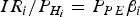 $\displaystyle{{I{R_i}} / {{P_{{H_i}}}}} = {P_{PE}}{\beta _i}$ is also a function of HPL and P mdi.
This study is aimed at providing a generalised algorithm to calculate HPL for all kinds of navigation service types, since the derivation of the worst case bias is regardless of the service types. The requirement of the NPA is adopted, where HPL is critical. Also, the multiple hypothesis structure is used here, which is also adopted in the design for the next generation RAIM structure ARAIM (Pervan et al., Reference Pervan, Pullen and Christie1998; ARAIM report, 2012). But the HPL presented here assumes a fixed  ${P_{{H_i}}}$, as opposed to ARAIM, which can accommodate different prior probabilities. However, it should be noted that the proposed method can be used in a more generalised RAIM scenario.
3. CURRENT METHODS TO CALCULATE HPL
Current methods to calculate HPL are based on approximations due to the complex calculation process to gain the exact probability and the worst case bias. The external reliability method (Brown and Chin, Reference Brown and Chin1998) was expanded by a random part to bound the random error (Angus, Reference Angus2007). In this method, two approximated distributions are used to calculate PPE. With the normal approximation,  $\sqrt {\vert\vert{{\tilde x}_H}\vert{\vert^2}} $ is approximated as a one degree Taylor series (Lee, Reference Lee1995)
 $$\sqrt {\nabla \tilde x_E^2 + \nabla \tilde x_N^2} + \displaystyle{{\nabla {{\tilde x}_E}} \over {\sqrt {\nabla \tilde x_E^2 + \nabla \tilde x_N^2}}} \left( {{{\tilde x}_E} - \nabla {{\tilde x}_E}} \right) + \displaystyle{{\nabla {{\tilde x}_N}} \over {\sqrt {\nabla \tilde x_E^2 + \nabla \tilde x_N^2}}} \left( {{{\tilde x}_N} - \nabla {{\tilde x}_N}} \right)$$
where  $\nabla {\tilde x_E}$ and
  $\nabla {\tilde x_N}$ are the non-centrality parameters of
  ${\tilde x_E}$ and
  ${\tilde x_N}$. The approximated variance is of a normal distribution
 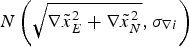 $N\left( {\sqrt {\nabla \tilde x_E^2 + \nabla \tilde x_N^2}, {\sigma _{\nabla i}}} \right)$ with
 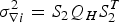 $\sigma _{\nabla i}^2 = {S_2}{Q_H}S_2^T $ which is then projected onto the direction of the faulty observation i with
 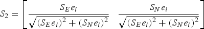 ${S_2} = \left[ {\displaystyle{{{S_E}{e_i}} \over {\sqrt {{{\left( {{S_E}{e_i}} \right)}^2} + {{({S_N}{e_i})}^2}}}} \; \; \; \displaystyle{{{S_N}{e_i}} \over {\sqrt {{{\left( {{S_E}{e_i}} \right)}^2} + {{({S_N}{e_i})}^2}}}}} \right]$ and Q H as the covariance matrix of
  ${\tilde x_H}$.
With the normal approximation, HPL BC under H i is (Angus, Reference Angus2007)
 $$HP{L_{BC1i}} = Hslope{1_i}{\delta _i} + K\left( {1 - \displaystyle{{{I}{{R}_{i}}} \over {2{{P}_{{{H}_{i}}}}}}} \right){\sigma _{\nabla i}}$$
where δ i is derived by the given P fai and 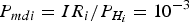 ${P_{mdi}} = \displaystyle{{{I}{{R}_{i}}} / {{{P}_{{{H}_{i}}}}}} = 10^{-3}$; K() is the inverse of the cumulative distribution function of a Gaussian random variable with zero mean and unit variance. The slope parameter is defined as the project matrix from the i th observation domain to the horizontal position error domain (Brown and Chin, Reference Brown and Chin1998) with
  ${S_{EN}} = {\left[ {\matrix{ {{S_E}} & {{S_N}} \cr}} \right]^T}$
 $$Hslope{1_i} = \sqrt {\displaystyle{{e_i^{T} S_{EN}^T {S_{EN}}{e_i}} \over {e_i^{T} P{Q_v}P{e_i}}}} $$
The second approximation is the chi-squared approximation, which is derived by the following inequality (Ober, Reference Ober1997)
 $$\sqrt {{\vert\vert{\tilde x}_H}\vert\vert^2} \le \sqrt {\displaystyle{1 \over {{\lambda _m}}}\tilde x_H^T Q_H^{ - 1} {{\tilde x}_H}} $$
where  $\tilde x_H^T Q_H^{ - 1} {\tilde x_H}$ is of chi-squared distribution with two degrees of freedom; λ m is the minimum Eigenvalue of
  $Q_H^{ - 1} $. With Equation (10), it can be concluded that the chi-squared approximation is always safe (Ober, Reference Ober1997).
In a similar way, HPLBC under H i with the chi-squared approximation is derived as
 $$HP{L_{BC2i}} = \sqrt {\displaystyle{1 \over {{\lambda _m}}}} \left[Hslope{2_i}{\delta _i} + \sqrt {{\chi ^2}\left( {2,1 - \displaystyle{{{I}{{R}_{i}}} \over {{{P}_{{{H}_{i}}}}}}} \right)} \right]$$
where δ i is derived by the given P fai and  ${P_{mdi}} = \displaystyle{{{I}{{R}_{i}}} / {{{P}_{{{H}_{i}}}}}} = 10^{-3}$;
  ${\chi ^2}\left( {2,1 - \displaystyle{{{I}{{R}_{i}}} \over {{{P}_{{{H}_{i}}}}}}} \right)$ represents the value at probability
  $1 - \displaystyle{{I{R_i}} \over {{P_{{H_i}}}}}$ with the central chi-squared inverse cumulative distribution function and two degrees of freedom; The slope factor for each hypothesis is
 $$Hslope{2_i} = \sqrt {\displaystyle{{e_i^T S_{EN}^T Q_H^{ - 1} {S_{EN}}{e_i}} \over {e_i^T P{Q_v}P{e_i}}}} $$
Another popular method is the weighted RAIM method (Walter and Enge, Reference Walter and Enge1995) designed for precision approach. The HPL WE is also tested here for NPA
 $$HP{L_{WEi}} = Hslope{1_i}{T_i} + K\left( {1 - \displaystyle{{{I}{{R}_{i}}} \over {2{{P}_{{{H}_{i}}}}}}} \right){\sigma _{HRMS}}$$
where  ${\sigma _{HRMS}} = \sqrt {\sigma _E^2 + \sigma _N^2} $ with σ E and σ N as the standard deviation of
  ${\tilde x_E}$ and
  ${\tilde x_N}$ respectively, and T i is derived with the given P fai as
  $K\left( {1 - \displaystyle{{{P_{fai}}} \over 2}} \right)$.
The solution separation method was proposed by Brenner (Reference Brenner1996) and applied in a multiple hypothesis structure (Pervan et al., Reference Pervan, Pullen and Christie1998), which is referred as the multiple hypothesis solution separation (MHSS) method
 $$HP{L_{PBi}} = \sqrt {HP{L_{Ei}}^2 + HP{L_{Ni}}^2} $$
where the east HPL is defined as
 $$HP{L_{Ei}} = {\sigma _{ssE}}{T_i} + K\left( {1 - \displaystyle{{I{R_i}} \over {2{P_{{H_i}}}}}} \right){\sigma _{iE}}$$
where σ ssE is the standard deviation of the east solution separation, which is equivalent to the east slope parameter  $Hslop{e_E} = \displaystyle{{\left\vert {{S_E}{e_i}} \right\vert} / {\sqrt {e_i^T P{Q_v}P{e_i}}}} $ (Blanch et al., Reference Blanch, Walter and Enge2010); σ iE is the standard deviation of the subset position error
  ${\tilde x_{iE}}$, which is derived with the ith observation removed in the estimator; the HPL for the north HPL Ni can be derived in a similar way with σ ssN as the standard deviation of the east solution separation also equivalent to the north slope parameter
  $Hslop{e_N} = \displaystyle{{\left\vert {{S_N}{e_i}} \right\vert} / {\sqrt {e_i^T P{Q_v}P{e_i}}}} $.
The method presented here to calculate HPL can be generalised for multiple faults with the relevant reliability measures for multiple faults described in Knight et al., (Reference Knight, Wang and Rizos2010). With current approximated HPL computation methods introduced as above, the exact HPL is pursued in the following sections, where the distribution of  $\sqrt {{\vert\vert{\tilde x}_H}\vert\vert^2} $ is analysed in Section 4 and the search for the worst case is studied in Section 5.
4. THE PROBABILITY OF THE HORIZONTAL POSITION ERROR
Two methods to calculate the exact probability PPE are studied: the Imhof approach (Imhof, Reference Imhof1961) and the DJ approach (DiDonato and Jarnagin, Reference DiDonato and Jarnagin1961; Milner and Ochieng, Reference Milner and Ochieng2010). They are chosen in consideration of the ability to control error tolerance for high accuracy, which is set at 10−9 for both implementations.
The Imhof approach is introduced as follows. With the correlation between the east and north error,  $\vert\vert{\tilde x_H}\vert{\vert^2}$ is not of a chi-squared distribution, but it is a sum of independent chi-squared variables (Ober, Reference Ober1997),
 $$\vert\vert{\tilde x_H}\vert\vert^2 = {\tilde y^T}S_{EN}^T {S_{EN}}\tilde y = \sum \nolimits_{\,j = 1}^2 {\lambda _j} \vert\vert q_j^T {\tilde y}\vert\vert^2$$
where  $\tilde y = y - A\hat x$ is the observation error vector, which is the difference between the real value and the estimated value; the Eigen-decomposition of the symmetric matrix
  $S_{EN}^T {S_{EN}}$ is D T∧ D with ∧ as the diagonal matrix, λ j as the non-zero diagonal elements, q j as the corresponding Eigen-vector, which form the columns of the orthogonal matrix D. Therefore,
  $\vert\vert{\tilde x_H}\vert{\vert^2}$ is a linear composition of independent chi-squared variables
  $\vert\vert q_j^{T} \tilde y\vert\vert^2$ with one degree of freedom and non-centrality parameter δ j. The probability of P PE can be computed with the Imhof method
 $$P\left\{ {\vert\vert{{\tilde x}_H}\vert{\vert^2} \gt HP{L^2}\vert{H_i}} \right\} = 0 \cdot 5 + \displaystyle{1 \over \pi} \int \nolimits_0^\infty \displaystyle{{sin \theta \left( u \right)} \over {u\rho \left( u \right)}}du$$
where θ(u) and ρ(u) are,
 $$\theta \left( u \right) = 0 \!\cdot \!5 \sum \nolimits_{\,j = 1}^2 [{\tan ^{ - 1}}\left( {{\lambda _j}u} \right) + {\delta _j}{\lambda _j}u{\left( {1 + \lambda _j^2 {u^2}} \right)^{ - 1}}] - 0 \!\cdot\! 5HP{L^2}u$$
 $$\rho \left( u \right) = \prod \nolimits_{\,j = 1}^2 \left[ {{{\left( {1 + \lambda _j^2 {u^2}} \right)}^{\scriptstyle{1 \over 4}}} exp \left( {\displaystyle{{{\delta _j}\lambda _j^2 {u^2}} \over {2 + 2\lambda _j^2 {u^2}}}} \right)} \right]$$
With the given error tolerance E U, the upper bound of the upper limit of integral U can be derived by,
 $${E_U} = \pi U \prod \nolimits_{\,j = 1}^2 \left[ {{\lambda _j}^{\scriptstyle{1 \over 2}} exp \left( {\displaystyle{{{\delta _j}\lambda _j^2 {U^2}} \over {2 + 2\lambda _j^2 {U^2}}}} \right)} \right]$$
With the east and north being de-correlated (Milner and Ochieng, Reference Milner and Ochieng2010), the DJ approach is applied, where a rectangular bound is defined to replace the cross area between an ellipse and a circular area to reduce the computational load (DiDonato and Jarnagin, Reference DiDonato and Jarnagin1961). The centre position of the circular area is the absolute value of the bias position after rotation of the correlation system. The given error tolerance is used to adjust the rectangular bound. The probability obtained by the integration of the cross area between the ellipse with the bivariate normal distribution and a circle is used as a reference which is referred as to the Bivariate Normal. Both methods and the two approximated ones (chi-squared, normal) are compared with the reference in Figure 1 with a single epoch example of seven visible satellites and a 12 m outlier on the first observation.

Figure 1. P PE as a function of HPL with different distributions.
As shown in Figure 1, the probabilities based on the Imhof and DJ approaches with 10−9 error tolerance are almost the same as the Bivariate Normal one. The chi-squared approximation is conservative with larger P PE, while the normal approximation is not. Similar conclusions can be found in Ober (Reference Ober1997). Using a standard Intel Core 2 Duo Processor E8400, the computational time per SV to calculate the P PE with different approaches is shown in Table 1.
Table 1. The average computational time of PPE per SV.

Therefore, the DJ approach should be used as it has higher accuracy and computational efficiency. It should also be noted that the Imhof approach is more general and can be used for higher dimensional cases.
5. THE APPROACHES TO CALCULATE THE HPL
The aim is to obtain the exact HPL solution to accommodate all possible bias, which is the HPL solution corresponding to the worst case bias with Equation (6). Besides the computation of the exact probability of PPE, the second issue arises when searching for the worst case in a boundary. The maximum HPL within a fixed interval is the corresponding solution. There is a one-to-one relationship between the non-centrality parameter and P mdi. The boundary was designed to be in the bias domain from 0 to the Minimal Detectable Bias (MDB) in Milner and Ochieng (Reference Milner and Ochieng2010), here the P mdi domain is used with the boundary as  $\displaystyle{{{I}{{R}_{i}}} / {{{P}_{{{H}_{i}}}}}} \sim 1$. With the lower boundary
  $\displaystyle{{{I}{{R}_{i}}} / {{{P}_{{{H}_{i}}}}}}$ given as 10−3 by Equation (6), the new criterion is expressed as
 $$\max {\,f_{HPL}}\left( {{P_{mdi}}} \right),{\rm subject \; to}\,{10^{ - 3}} \lt {P_{mdi}} \lt 1$$
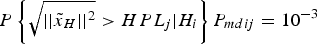
where f HPL(P mdi) stands for the HPL as a function of P mdi, which is expressed by the non-linear equation  $P \{ \sqrt {\vert\vert{\tilde x}_H \vert\vert^{2}} \gt HPL \vert H_i \} P_{mdi} = 10^{ - 3}$ with given integrity risk. To obtain the best solution, the iterative method in Milner and Ochieng (Reference Milner and Ochieng2010) is introduced first, followed by an improved iterative method, and finally an optimisation method is proposed, which are all compared in terms of accuracy and efficiency.
With a closed boundary, it is guaranteed that there is always an extreme value. The mechanism is shown in Figure 2, with the decrease of P mdi within the range, the non-centrality parameter is increased from δ a to δ c. The corresponding HPL increases from HPLa to HPLb and then decreases to HPLc. Therefore, a search is needed to obtain the worst case.
Figure 2. Illustration of the search method.
To search the worst bias in the P mdi range, it is necessary to define the worst case first. As shown in Figure 3, the worst integrity risk happens when P mdi is 15·01%, which is the same for the worst HPL in Figure 4. The worst case happens at the same P mdi point because the input HPL is 5·197 m in Figure 3, corresponding to the worst HPL in Figure 4, and vice versa. Still, it is illustrated that there are two ways to define the worst case: the maximum integrity risk with given HPL and the maximum HPL with given integrity risk.
Figure 3. P md and Integrity Risk.
Figure 4. P md and HPL.
5.1. The Original Iterative Method
A procedure is defined in Milner and Ochieng (Reference Milner and Ochieng2011) with the maximum integrity risk as the worst case to calculate the ideal VPL, which can be applied to HPL as well, and referred to as the Iterative A method. There are two iterative search loops over the inner loops covering the bias range and the outer one as the input HPL range. For each inner loop, there is a worst bias point that has the maximum integrity risk with the given input HPL. For all the input HPL values in the outer loop, the one that generates the maximum integrity risk closest to the given integrity risk is the desired value. The process is described as follows: in the outer loop, an upper value U is chosen to decide the range 0 <HPL <U with HPLk as the value at step k. The P mdi range 10−3 <P mdi <1 is used in the inner loop with P mdij as the value at step j. In each step j, the integrity risk 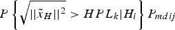 $P \left\{ \sqrt {\vert\vert{\tilde x}_H \vert\vert^{2}} \gt HP{L_k} \vert H_i \right\} P_{mdij}$ is calculated and the maximum value in the inner loop is chosen. The HPLk that generates the maximum integrity risk which is the closest to 10−3 is the final result. Therefore, the accuracy of the results and computational time is dependent on the number of steps in two loops.
5.2. The New Iterative Method
The iterative method is designed to derive each HPL value corresponding to each P mdij with the non-linear equation and the maximum one is the final result with the worst case bias. The procedure is as follows:
1) The P mdi range is divided by the number of steps N with P mdij as the value at step j.
2) The HPL j corresponding to each P mdij are derived by equation
 $P \left\{ \sqrt {\vert\vert{\tilde x}_H \vert\vert^{2}} \gt HP{L_j} \vert H_i \right\} P_{mdij}= 10^{ - 3}$, where an optimisation tool to solve non-linear equations is used.
3) The maximum HPL j is therefore the desired result.
In this way, the outer loop is removed, and both the accuracy of the results and computational time is dependent on the number of steps in a single search loop. This method is referred to as the Iterative B method.
5.3. The Optimisation Method
To gain a HPL value with higher accuracy and computational efficiency, an optimisation algorithm is used to find the maximum value within a fixed interval. The MATLAB implementation fminbnd is used to find the single local minima with a continuous function of one variable, which is based on golden section search and parabolic interpolation (Forsythe et al., Reference Forsythe, Malcolm and Moler1976). The criterion is then adapted to be used in this optimisation tool, where P mdi is treated as the unknown parameter that needs to be solved and HPL is expressed by the unknown P mdi with 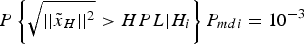 $P \left\{ \sqrt {\vert\vert{\tilde x}_H \vert\vert^{2}} \gt HPL \vert{H_i} \right\} P_{mdi}= 10^{ - 3}$. The maximisation problem is adapted as a minimisation problem by subtracting the HPL function from a large number (e.g. 100-HPL). The optimisation tool is used to find the P mdi value that has the maximum HPL value. The termination tolerance, which is the norm of the difference of two consecutive solution vectors during the iterative optimisation process, is set as 10−8 to guarantee the accuracy of the final results. The initial value is set according to experiment data to speed up the solving process. The procedure of this method is described as below:
1) The function to compute P PE is implemented with the DJ approach as f 1. The input parameters include Q H, HPL and the non-central parameter in
${\tilde x_E}$ and ${\tilde x_N}$ as $Hslop{e_E} \,\ast\, {\delta _i}$, $Hslop{e_N} \,\ast\, {\delta _i}$. The output is P PE.2) The function to compute HPL is implemented as follows:
a. Define an initial value x 0 and a search range P mdi ∈ [10−3, 1 ].
b. Define other input parameters: T i,
$I{R_i}/{P_{{H_i}}}$, P fai and the Eigenvalues of Q H.c. A function f 2 is defined to compute the equation
$\scriptstyle{{f_1}} - I{R_i} \ast \displaystyle{{P_{mdi}} \over {P_{H_i}}} = 0$ with fsolve, where P mdi is the input variable and HPL is the output variable. The initial value x 0 and the termination tolerance are defined beforehand.d. 100 − HPL as a function of variable P mdi from f 2 is then used in fminbnd as the function to be minimised within a fixed interval of P mdi ∈ [10−3, 1].
e. The solution from fminbnd is the worst case P mdi, and the corresponding HPL is the final solution, which is derived with the equation in f 2.


Although in theory there will always be a solution, the convergence of the optimisation algorithm depends on the proper choice of the initial value and the termination tolerance. Besides, to avoid discontinuity, the new iterative method is used in practice whenever there is no extreme value found in the optimisation algorithm.
6. NUMERICAL RESULTS
Comparing the new iterative method with the original one, the result would be close to the theoretical value if the steps were close to infinite. However, the number of steps cannot afford to be too big with the requirement of TTA in RAIM – the integrity information would not be transmitted to users in time. Normally, TTA should be within a few seconds, for example the TTA requirement for the LPV-200 service is 6·2 seconds. With a smaller number of steps, it is observed that the accuracy of the results is not necessarily better when using more steps. The reason lies in the uncertainty of the location of the worst case and the step size. An example is given in Figure 5 with various steps: 5, 10, 20 and 30. The worst case under each steps are marked with a rectangular box. It can be seen that the HPL using 20 steps is closer to the correct HPL than using 30 steps. With all the uncertainties, it is concluded that the iterative methods are not only too time consuming, but also lack sufficient accuracy.
Figure 5. The uncertainty in iterative methods with the number of steps.
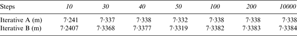
Results from two iterative methods with different steps for P mdi range are compared in Table 2, where the HPL is ranged between 0~50 m with 50,000 steps to achieve the accuracy of 0·001 m in the Iterative A method. The result from the optimisation method (7·3384 m) is used as the reference point.
Table 2. Different HPL values in one epoch with various steps.
In Table 2 with the Iterative B method, the result with 40 steps is closer to the reference value than with 50 steps. Therefore, it is concluded that the accuracy of the results is not necessarily getting better with larger steps, which is consistent with the analysis in Figure 5. But with an extremely large number of steps (10,000), the value is the same as the reference value. Also, with the number of steps larger than 100, the result stays relatively stable at the accuracy of 10−4. With an additional search loop in the Iterative A method, the HPL precision is constrained by the outer number of steps with 0·001 m accuracy. Yet, this accuracy is not reliable since it is still susceptible to the uncertainty caused by the search in the β i range with the example of the results using 40 and 50 steps in Table 2. Therefore, it is concluded that introducing another search loop in the Iterative A method does not enable the control of the accuracy of the results.
The Iterative B method with 150 steps and 10 steps are compared with the optimisation method in Figure 6 using data of the GPS observations captured on the UNSW campus within 24 hours. It is assumed that the error is of standard normal distribution without correlation.
Figure 6. The iterative methods and the optimisation approach for the new HPL.
It is shown in Figure 6 that the results from the iterative method with 150 steps are very close to the results from the optimisation method. However, the results from the iterative method with 10 steps are smaller than the optimisation method at the scale of 0·1 m. Therefore the accuracy of the results from the iterative method is lower and the conservativeness is not guaranteed, depending on the number of search steps, while the optimisation method is more reliable.
Using an Intel Core 2 Duo Processor E8400, the average computational time per epoch is shown in Table 3. For both iterative methods, the total number of search step is 100 in the P mdi range. HPL is ranged between 0~50 m with 500 steps with 0·1 m accuracy.
Table 3. The average computational time of HPL in one epoch.

With 100 search steps, the results from the Iterative B and optimisation methods are similar, but it is shown in Table 3 that the optimisation method is faster with less than half of the time used per SV than the Iterative B method. The Iterative A method consumes around 20 s per epoch, while the optimisation method is more promising for use in real time applications. Also, an approach to limit the search region was designed in Milner (Reference Milner2009) as well as Milner and Ochieng (Reference Milner and Ochieng2010) to improve the computational efficiency. But since the two loops impose a considerable computational burden, such improvement is less obvious than the Iterative B method in this test.
All existing approximated algorithms to calculate HPL are examined by comparing with the new optimisation value in Figure 7.
Figure 7. The new HPL and other approximated HPLs.
As shown in Figure 7, the two HPL BCs are conservative, while HPL WE has values higher than the new HPL. Although the normal approximation distribution is not safe compared with the exact distribution as shown in Figure 1, the HPL BC2 based on it is still conservative.
To quantify the performance improvement with the new HPL, the simulation for worldwide availability distribution is set up as follows. The almanac data for the standard 24 satellite GPS constellation and the 27 satellite Galileo constellation was used respectively to determine the geometry at each location with a 5 × 5 degree grid on the world map at 50 m altitude. The error model is adopted from GEAS (2008) for ARAIM, and a bias term was added to gain more conservative results. The values for the nominal bias and the maximum bias were 0·1 m and 0·75 m separately. The User Range Error and User Range Accuracy were 0·25 m and 0·5 m. The risk definition is the multiple hypothesis requirements as defined in Section 2. Results of HPL at each location are computed every 10 min over the 24 hour duration. The mask angle of GPS is set to be 5°. The availability was determined by comparing each HPL value with the alert limit (40 m) for each location. The percentage of having over 99% availability over this time is shown worldwide. The simulation software is based on the MATLAB Algorithm Availability Simulation Tool provided by Stanford University.
It is shown in the Figures 8–11 and Tables 4 and 5 that the performance is improved with 99% availability worldwide, especially when the alert limit is tighter in Table 5 (HAL set to be an arbitrary 35 m). Although HPL PB showed a lower value than HPL BC1 in Figure 7, the service availability is higher than HPL BC1 with 24 GPS and lower with 27 Galileo. From this example we can conclude that there is no definite conclusion comparing the size of HPL PB and HPL BC1, which is dependent on the geometry between satellites and users.
Figure 8. 99% Availability with HPLBC1, 24 GPS.
Figure 9. 99% Availability with HPLBC2, 24 GPS.
Figure 10. 99% Availability with HPLPB, 24 GPS.
Figure 11. 99% Availability with new HPL, 24 GPS.
Table 4. 99% 40 m HAL Availability with Different Algorithms.

Table 5. 99% 35 m HAL Availability with Different Algorithms.

7. CONCLUDING REMARKS
It has been shown that the new approach to calculate HPL has high accuracy and computational efficiency, and therefore service availability can be improved in RAIM and potentially in other Global Navigation Satellite System (GNSS) aviation operational applications. Also, the computation of the new iterative method is faster than the old method. With the exact HPL value validated, the conservativeness of current HPLs are analysed. It is proved that the chi-squared distribution is a safe choice to approximate the exact distribution of horizontal position error, while the normal approximation is not. The results have shown that HPL BC and HPL PB are conservative, while HPL WE does not meet the theoretical integrity requirement. With the optimisation method given in the MATLAB toolbox, further efforts can be made to customize an optimisation method for this specific problem to maximise the computational efficiency. Although there is no outage of discontinuity with the optimisation method in this paper, the proposed method should be further investigated to make sure that 100% convergence can be guaranteed. For the same purpose, the idea proposed by Milner (Reference Milner2009) to limit the search region may be incorporated in the current proposed method for further study.