


1. INTRODUCTION
Mars missions remain an attractive topic in deep space exploration. Mars can also offer gravity assist to probes with destinations such as Jupiter (Jiang et al., Reference Jiang, Baoyin and Li2012) and asteroids (Chen et al., Reference Chen, Baoyin and Li2014), so Jupiter or asteroids probes may enter orbit near to Mars. Navigation of Mars probes is essential to successfully implement Mars missions. Autonomous navigation, where the spacecraft performs navigation functions itself, can overcome the drawbacks of traditional observation techniques and reduce dependence on Earth-based tracking stations such as the Deep Space Network (DSN) or Very Long Baseline Interferometry (VLBI). Several different measurement methods for autonomous navigation have been proposed according to measurement type, such as optical measurement and X-ray pulsar measurement (Downs, Reference Downs1974; Duxbury et al., Reference Duxbury, Born and Jerath1974; Chester and Butman, Reference Chester and Butman1981; Chory et al., Reference Chory, Homan and LeMay1986; Hicks and Wiesel, Reference Hicks and Wiesel1992; Sheikh, Reference Sheikh2005; Christian and Lightsey, Reference Christian and Lightsey2010, Deng et al., Reference Deng, Hobbs, You, Li, Keith, Shannon, Coles, Manchester, Zheng, Yu, Gao, Wu and Chen2013; Liu et al., Reference Liu, Ma, Tian, Kang and Paul2010).
X-ray pulsar-based navigation is a developing method and has recently attracted increasing attention. The National Aeronautical and Space Agency (NASA) has been considering the feasibility of using X-ray pulsars as navigation source for spacecraft navigation for some years. In 1968, Bell and Hewish discovered pulsars, which emit very stable periodic signals. The period of a pulsar is so stable that the signal could be used as a precise clock. According to this property of pulsars, Downs (Reference Downs1974) presented a method of navigation for orbiting spacecraft based on radio signals from pulsars. Chester and Butman (Reference Chester and Butman1981) proposed to use the X-ray band emitted from pulsars as an improved option for Earth satellite navigation. Since the 1990s, analyses have concluded that the size of the sensor that receives X-ray signals from a pulsar need only be of the order of 0·1 m2, which would be significantly smaller than both the antennas and telescopes that receive radio signals from a pulsar. Even so, it is difficult for a probe to load several X-ray detectors for navigation because of its capacity. So, it is possible that only one X-ray detector is loaded on a probe. Usually, at least three X-ray pulsars are needed for geometry navigation. But with the help of dynamic orbit determination methods for navigation, one or two X-ray pulsar detectors onboard a probe may also be feasible. Sometimes, the navigation accuracy and reliability of single X-ray pulsar measurement is very low due to poor observability. In addition, time transfer errors will also result in poor navigation.
On the other hand, optical measurement autonomous navigation has been an attractive research focus of space missions. Many methods have been proposed in recent years (Bhaskaran et al., Reference Bhaskaran, Riedel and Synnott1998; Reference Bhaskaran, Riedel, Synnott and Wang2000; Chausson et al., Reference Chausson and Delavault2003; Mastrodemos et al., Reference Mastrodemos, Kubitschek and Synnott2005; Stastny and Gellert, Reference Stastny and Gellert2008; Paluszek et al., Reference Paluszek, Mueller and Littman2010; Christian and Lightsey, Reference Christian and Lightsey2010; Ma et al., Reference Ma, Jiang and Baoyin2015). Optical measurement autonomous navigation has been tested successfully in several recent deep space missions such as the Deep Space 1, the STARDUST mission and the Deep Impact mission. Phobos and Deimos, the two natural moons of Mars, are important optical navigation information sources available for Mars missions. Duxbury et al. (Reference Duxbury, Born and Jerath1974) proposed a method of viewing Phobos and Deimos to navigate Mariner 9. However, during the phase of probe orbits near to Mars, the ephemeris biases of Martian moons are crucial to navigation accuracy. The ephemeris accuracy of the two Martian moons could be still several kilometres according to research by Lainey et al. (Reference Lainey, Dehant and Patzold2007). Moreover, due to the irregular shapes of Martian moons and the different phase angle of sunlight, the difference between barycentre and centre of brightness of the Martian moons is considerable. As a result, the apparent position errors of the two Martian moons may exceed several kilometres. Therefore, it is very difficult to attain high navigation accuracy by only using on board images of Phobos and Deimos during the Mars orbit phase.
2. AUTONOMOUS NAVIGATION ALGORITHM
In order to improve autonomous navigation accuracy and reliability of Mars probes during the Mars orbiting phase, an integrated navigation method using X-ray pulsar measurement and optical data of viewing Martian moons is proposed in this paper (Figure 1). The Mars centre is set as reference origin of Time Of Arrival (TOA) in this paper.

Figure 1. The scenario of Single X-ray Pulsar Measurement and Martian Moon optical measurement.
2.1. System dynamics
During the phase orbiting Mars, the probe dynamics should be established in the J2000.0 Mars-centre inertial coordinate system. The dynamical model can be written as
 $$ \ddot{\bi r} = {{\bi a}_0} + {{\bi a}_{{\rm ns}}} + {{\bi a}_{{\rm nbody}}} + {{\bi a}_{{\rm srp}}} + {{\bi a}_{{\rm drag}}} + {{\bi a}_{{\rm thrust}}} + {{\bi a}_\varepsilon}$$
For a Mars probe, besides Mars body centre gravitational force a 0, other perturbation forces include Mars’ non-spherical gravitational perturbation a ns according to the gravity field of Mars GMM-2B (Lemoine et al., Reference Lemoine, Smith, Rowlands, Zuber, Neumann, Chinn and Pavlis2001), the third body gravitational perturbations from the Sun and other major planets a nbody, solar radiation pressure a srp. Martian atmosphere drag perturbation a drag should also be considered for very low orbits. a thrust is the thrust force of the probe.
In addition, a ε is the sum of other forces acting on a probe, which are too small to count, such as the gravitational forces of Martian moons. The RKF7(8) algorithm is applied for orbit propagation of this dynamical model.
Because an on board computer cannot cope with an over-large load, the dynamical model of on board navigation must be simplified. In order to analyse how the dynamics model errors affect navigation precision, a precise dynamical model (model-1) is set as a criterion and a simplified model (model-2) is used for state estimation of on board navigation, as shown in Table 1.
Table 1. Different options of precise dynamics model and simplified model.

2.2. X-ray pulsar measurement model
For X-ray pulsar measurement, the X-ray sensor on board a probe detects the photons emitted from pulsars to determine the TOA of X-ray signal pulses. Meanwhile, the TOA of signal pulses at reference origin can be accurately provided by a timing model. Usually, the reference origin is selected as the Solar System Barycentre (SSB) because of the requirements of an inertia frame system. The TOA difference (ΔTOA) between a measured pulse arrival time at probe sensor and predicted time at the SSB origin can be used for navigation.
In order to compare a measured pulse arrival time at a probe with predicted time at the SSB origin, the probe must project TOA onto the SSB origin. This comparison requires time to be transferred from the probe to the SSB. The geometric and relativistic effects must be taken into account in the transfer process. These light ray paths can be determined using the existing theory of general relativity effects of the solar system (Richter and Matzner, Reference Richter and Matzner1983). Sheikh (Reference Sheikh2005) and Sheikh et al. (Reference Sheikh, Pines, Rayp, Wood, Lovellette and Wolff2006) present an accurate model Equation (2) and simplified model Equation (3) to transfer detected arrival times to the SSB origin.
In Equations (2) and (3), t SSB is the pulse TOA at the SSB; t SC is the TOA at probe; c is the speed of light; μ s is the gravitational constant of the Sun; μ k is the gravitational constant of the planet of the solar system; b is the position vector of the SSB origin relative to the Sun; b k is the position vector of the planet relative to the Sun. In Equation (2), n SSB is the unit direction vector from the SSB to the pulsar; n SC is the unit direction vector from the probe to the pulsar source; D is the position vector from the Sun to the pulsar source, p is the position vector from the Sun to the spacecraft; and p x , D x , D y are the axis components of p and D . In Equation (3), n is the unit direction vector from the SSB to the pulsar; r SC is the position vector from the SSB to the probe, and D 0 is the range from the SSB to the pulsar source; PBss is the number of planets that should be taken into account.
 $$\eqalign{({t_{SSB}} - {t_{SC}}) &= \displaystyle{1 \over c}{{\bi n}_{SSB}} \cdot ({\bi D} - {\bi b}) - \displaystyle{1 \over c}{{\bi n}_{SC}} \cdot ({\bi D} - {\bi p}) \cr &\quad - \sum\limits_{k = 1}^{P{B_{SS}}} {\displaystyle{{2{\mu _k}} \over {{c^3}}}\ln} \left \vert {\displaystyle{{{{\bi n}_{SSB}} \cdot {{\bi b}_k} + {b_k}} \over {{{\bi n}_{SSB}} \cdot {{\bi D}_k} + {D_k}}}} \right \vert + \sum\limits_{k = 1}^{P{B_{SS}}} {\displaystyle{{2{\mu _k}} \over {{c^3}}}\ln} \left \vert {\displaystyle{{{{\bi n}_{SC}} \cdot {{\bi p}_k} + {\,p_k}} \over {{{\bi n}_{SC}} \cdot {{\bi D}_k} + {D_k}}}} \right \vert \cr &\quad + \displaystyle{{2\mu _S^2} \over {{c^5}D_y^2}} \left\{ {\matrix{ {{{\bi n}_{SSB}} \cdot ({\bi D} - {\bi b})\left[ {1 + {{\bigg(\displaystyle{{{{\bi n}_{SSB}} \cdot {\bi D}} \over D}\bigg)}^2}} \right]} \cr { + 2({{\bi n}_{SSB}} \cdot {\bi D})\bigg(\displaystyle{b \over D} - 1\bigg)} \hfill\cr { + {D_y}\left[ {\arctan \bigg( \displaystyle{{{\,p_x}} \over {{D_y}}} \bigg) - \arctan \bigg( \displaystyle{{{D_x}} \over {{D_y}}} \bigg) } \right]} \cr}} \right\} \cr &\quad - \displaystyle{{2\mu _S^2} \over {{c^5}D_y^2}} \left\{ {\matrix{ {{{\bi n}_{SC}} \cdot ({\bi D} - {\bi p})\left[ {1 + {{ \bigg( \displaystyle{{{{\bi n}_{SC}} \cdot {\bi D}} \over D} \bigg) }^2}} \right]} \cr { + 2({{\bi n}_{SC}} \cdot {\bi D}) \bigg( \displaystyle{\,p \over D} - 1 \bigg) } \hfill\cr { + {D_y}\left[ {\arctan \bigg( \displaystyle{{{\,p_x}} \over {{D_y}}} \bigg) - \arctan \bigg( \displaystyle{{{D_x}} \over {{D_y}}} \bigg) } \right]} \cr}} \right\}}$$
 $$\eqalign{ c({t_{SSB}} - {t_{SC}}) &= {\bi n} \cdot {{\bi r}_{SC}} + \displaystyle{1 \over {2{D_0}}}[{({\bi n} \cdot {{\bi r}_{SC}})^2} - {\bi r}_{SC}^{\,2} + 2({\bi n} \cdot {\bi b})({\bi n} \cdot {{\bi r}_{SC}}) - 2({\bi b} \cdot {{\bi r}_{SC}})] \cr & \quad + \sum\limits_{k = 1}^{P{B_{ss}}} {\displaystyle{{2{\mu _k}} \over {{c^2}}}\ln \left \vert {\displaystyle{{{\bi n} \cdot {{\bi r}_{SC}} + {r_{SC}}} \over {{\bi n} \cdot {{\bi b}_k} + {b_k}}} + 1} \right \vert}}$$
The time transfer accuracy of the accurate algorithm Equation (2) is of the order of nanoseconds, and the time transfer accuracy of simplified algorithm Equation (3) is of the order of microseconds near to Mars. An accuracy of several microseconds will result in a position error of the order of kilometres, so the simplified time transfer algorithm Equation (3) cannot achieve high accuracy navigation results. The accurate time transfer algorithm Equation (2) can achieve high accuracy navigation results, but it is very difficult for on board navigation use because of its complexity. In addition, the range from the Sun to the pulsar source may exceed ten thousand light years away, so it needs at least quadruple precision (128 bits of floating point representation). Otherwise, the numerical error of computing will result in poor navigation accuracy. For example, using double precision (64 bits), the numerical error of TOA may exceed a few microseconds. But, practically, allocation of computers with capability of high numerical precision on board is very expensive.
In order to solve the problem of time transfer accuracy, for a probe orbiting Mars, we can set Mars’ centre as reference origin. But Mars is orbiting the Sun, so the TOA at Mars is variable owing to the Martian motion. Fortunately, we can compute comparisons of the TOA at Mars with the TOA at the Sun for the same pulsar sources in advance. The high accuracy numerical arithmetic program (such as quadruple precision) and the accurate time transfer algorithm Equation (2) can be used in this process. The motion of the pulsars should be taken into account as follows
 $${\bi D} = {{\bi D}_0} + {\bi V}\Delta t$$
Here, D 0 is the position vector of a pulsar at initial epoch time, and V is the proper motion of the pulsar.
The TOA values of X-ray pulsar navigation sources at Mars’ centre should be loaded onto the on board computer in advance, of which accuracy is of the order of nanoseconds according to Equation (2).
In on board navigation computing, the comparisons of the TOA at a probe with the TOA at Mars’ centre should be calculated by the simplified time transfer algorithm. So, the X-ray pulsar measurement model in the Mars centre inertial coordinate is derived from Equation (5).
 $$c({t_{Mars}} - {t_{SC}}) = c({t_{SSB}} - {t_{SC}}) - c({t_{SSB}} - {t_{Mars}})$$
Since the position vector from the Sun to the probe r SC and the position vector from the Sun to Mars r M are close, the expression may be further simplified as,
 $$c({t_{Mars}} - {t_{SC}}) = {\bi n} \cdot ({{\bi r}_M} - {{\bi r}_{SC}}) = {\bi n} \cdot {\bi r}$$
Here, n is the unit direction vector from Mars to the pulsar, and r is the position vector from Mars to the probe. n is determined by right ascension α and declination δ of the pulsar as follows,
 $${\bi n} = \left( {\matrix{ {{n_x}} \cr {{n_y}} \cr {{n_z}} \cr}} \right) = \left( {\matrix{ {\cos \alpha \cos \delta} \cr {\sin \alpha \cos \delta} \cr {\sin \delta} \cr}} \right)$$
In order to analyse the error coming from simplifying Equation (5) to Equation (6), the TOA of two samples which are located 300 km and 20,000 km away from Mars respectively are computed over the period of three Mars years. The result of Equation (5) is computed by quadruple precision and that of Equation (6) is computed by double precision.
Figure 2 gives the comparison results between Equation (5) and Equation (6). Figure 2 shows that the maximum TOA error of the orbit location with Mars 300 km away between Equation (5) and with Equation (6) is less than 0·7 ns, and the maximum TOA error of the orbit location with Mars 20,000 km away is less than 3 ns. So, the method using simplified Equation (6) to compute TOA is practicable.
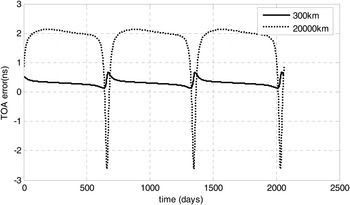
Figure 2. The error of the simplified TOA method.
Equation (6) is the X-ray pulsar measurement model in the Mars centre inertial coordinate, which is very simple and convenient for on board computing. The partial derivative of the X-ray pulsar measurement with respect to state variables is as follows
 $$\displaystyle{{\partial c({t_{Mars}} - {t_{SC}})} \over {\partial {\bi r}}} = \left( {\matrix{ {{n_x}} \cr {{n_y}} \cr {{n_z}} \cr}} \right)$$
2.3. Optical measurement
If there are a Martian moon and more than three background stars caught in an image taken by the on board optical sensor, the angles between the Martian moon and the background stars can be obtained. The unit vector of the Martian moon n p (x np, y np, z np) can be obtained in the probe centre inertial coordinate system from more than three angles. The right ascension α and declination δ are:
 $$\alpha = \arctan\! \left( {\displaystyle{{{y_{{\rm np}}}} \over {{x_{{\rm np}}}}}} \right),\quad \delta = \arcsin\! \left( {\displaystyle{{{z_{{\rm np}}}} \over {{r_{{\rm np}}}}}} \right)$$
In the Mars centre inertial coordinate system, r (x, y, z) is the position vector of the probe, and r m(x m, y m, z m) is that of the Martian moon. Then, r p(x p, y p, z p) = r m– r is the position vector of the Martian moon in the probe centre inertial coordinate system, and the measurement model of right ascension α and declination δ are obtained.
 $$\alpha = \arctan \left( {\displaystyle{{{y_{\rm p}}} \over {{x_{\rm p}}}}} \right),\quad \delta = \arcsin \left( {\displaystyle{{{z_{\rm p}}} \over {{r_{\rm p}}}}} \right)$$
The partial derivative of right ascension α and declination δ with respect to state variables are as follows
 $$\displaystyle{{\partial \alpha} \over {\partial {\bi r}}} = \displaystyle{1 \over {x_{\rm p}^2 + y_{\rm p}^2}} \left( {\matrix{ y \cr { - x} \cr 0 \cr}} \right),\quad \displaystyle{{\partial \alpha} \over {\partial \dot{\bi r}}} = {\bf 0}$$
 $$\displaystyle{{\partial \delta} \over {\partial {\bi r}}} = \displaystyle{1 \over {r_{\rm p}^2 \sqrt {x_{\rm p}^2 + y_{\rm p}^2}}} \left( {\matrix{ { - {x_{\rm p}}z} \cr { - {y_{\rm p}}z} \cr {x_{\rm p}^2 + y_{\rm p}^2} \cr}} \right),\quad \displaystyle{{\partial \delta} \over {\partial \dot {\bi r}}} = {\bf 0}$$
2.4. Estimation methods
Generally, for space navigation, the sequential processing algorithm is usually used for on board estimation. So, two sequential processing algorithms including Extended Kalman Filter (EKF) and Unscented Kalman Filter (UKF) are selected to be applied and compared in this paper. One can refer to the pioneering work of Kalman (Reference Kalman1960) and Kalman and Bucy (Reference Kalman and Bucy1961) for EKF and many improvements have been proposed (Bar-Itzhack and Medan, Reference Bar-Itzhack and Medan1983). EKF is still adopted extensively in autonomous navigation (Xiao et al., Reference Xiao, Wu, Fu and Zhang2015). The UKF is a new filtering algorithm for nonlinear systems invented by Julier and Uhlmann (Reference Julier and Uhlmann1997). The state transition matrix and the Jacobi matrices of the dynamical equations and observation equations, necessary to EKF, are not required for UKF. The key point of the UKF is based on an Unscented Transformation (UT) which uses a set of appropriately chosen weighted points to parameterise the mean and covariance of the probability distributions. A detailed description of the UKF theory can be found in Julier and Uhlmann (Reference Julier and Uhlmann2004).
3. SIMULATION
3.1. Scenario Setting
We set two scenarios as samples to substantiate our methods. The first example is a Low Mars Orbit (LMO) with a high-inclination scenario (a = 3696 km, e = 0·001, i = 75°) and the second is a High Mars Orbit (HMO) with a low-inclination scenario (a = 20430 km, e = 0·001, i = 0°) in a Mars-Centre inertia system. Table 2 lists the initial positions and velocities of the probes in the two scenarios, which are projected onto the J2000·0 Mars-equator coordinate system.
Table 2. Orbit parameters in Mars-Centred J2000 Coordinate system (Epoch Time (TDT) 2016–01–01 00:00:00).

In order to analyse the propagating errors of the simplified model, the position differences between model-1 and model-2 are compared in Figures 3 and 4. The figures show that the position errors due to dynamics model error of HMO are several tens of metres for three days’ propagation. As to LMO, the position error for three days’ propagation is several tens of kilometres.

Figure 3. LMO propagation difference between the simplified model and precise model.

Figure 4. HMO propagation difference between the simplified model and precise model.
A single X-ray pulsar sensor is loaded and its direction can be adjusted to point to an arbitrary pulsar, so a few pulsars with different right ascension and declination that scatter on the celestial sphere are adequate to be observed for navigation. In this paper, three pulsars are selected as navigation sources, and their parameters are listed in Table 3. Δα and Δδ are the direction error of the pulsars in the simulation. Liu et al. (Reference Liu, Ma, Tian, Kang and Paul2010) analysed an X-ray pulsar navigation method for spacecraft with pulsar direction error.
Table 3. Orbit parameters of low-inclination scenario.

3.2. Visibility Analysis
Suppose the attitude mode of a probe orbiting Mars is the Mars nadir pointing mode (the Z axis always directs towards Mars’ centre), and the X-ray pulsar sensor loaded on –Z panel of the probe. In the attitude mode, if the angle between the –Z axis (directs to zenith) and the vector from a pulsar to the probe is less than 90°, the pulsar can be observed. If more than two pulsars were observed, the pulsar with the smaller angle will be selected to be observed. Also, the Sun should be out of the field of view of the navigation X-ray sensor. According to above visibility condition, three pulsars (B0531 + 21, B1821 – 24, B1937 + 21) can guarantee that at least one of them is observed by the probe at all times.
As for optical measurement, there are four factors that affect the observation of the probe to Martian moons: (1) the probe and Martian moons are not obstructed in line by Mars; (2) Martian moons are not in the shadow of Mars; (3) Martian moons must reflect enough solar light to the probe; and (4) the Sun and Mars are out of the field of view of the navigation optical sensor. The effect of the probe attitude on visibility is not taken into account for optical measurement, because the probe can adjust its sensor direction to adapt to suit the observation object.
3.3. Simulation conditions
The criterion data simulation is carried out by propagating the orbit from initial state under precise dynamical model (model-1). The simplified dynamics model (model-2) is used for navigation. The difference between the precise model and the simplified model is taken as model error. The ephemeris of Mars and Martian moons are obtained through the Jet Propulsion Laboratory's online website: http://ssd.jpl.nasa.gov/horizons.cgi.
The simulated X-ray pulsar measurement stochastic error is 300 m (1σ) and bias is 300 m. At present, only the measurement of B0531 + 21 can reach this accuracy. But with the development of a more sensitive on board sensor and larger aperture radio telescope for finding and measuring pulsars such as the FAST project (Five hundred metres Aperture Spherical Telescope) in China, more pulsars with precise measurement will be found in the future. The simulating measurement errors are in accord with 1 μs of the TOA random error and 0·1 μs bias, and the pulsars position errors are given by Δα and Δδ in Table 3.
To simulate the measurement error, the optical measurement error is set according to the following equation.
 $$\sigma = {\sigma _1} + \arctan \Big(\displaystyle{{{\sigma _{Eph}}} \over {\Delta R}}\Big) + \arctan \Big(\displaystyle{{{R_{moon}}} \over {\Delta R}}\Big)\sin \displaystyle{\psi \over 2}$$
Where σ 1 is the random error with Gaussian distribution of 0·01°, which includes measurement noise and the errors of the stellar location of background stars. σ Eph is the Martian moon ephemeris error of 10 km, ΔR is the range from probe to Martian moon, R moon is the approximate radius of the Martian moon of 5 km and ψ is the phase angle from Martian moon to the Sun and probe.
Because the stellar location accuracy of the current stellar catalogue is far higher than 1″ (Hog et al., Reference Hog, Fabricius, Makarov, Urban, Corbin, Wycoff, Bastian, Schwekendiek and Wicenec2000), the effect of stellar location accuracy on navigation accuracy is included in random error (σ 1) of 0·01°.
In the filter process, the initial position and velocity uncertainties are set as 10 km and 5 m/s respectively for the simulation samples. The initial state covariance and the measurement noise covariance used for the navigation filter are as follows:
 $${{\bi P}_0} = {\rm diag}[{(10{\rm km})^2},{(10{\rm km})^2},{(10{\rm km})^2},{(5{\rm m}/{\rm s})^2},{(5{\rm m}/{\rm s})^2},{(5{\rm m}/{\rm s})^2}]$$
 $${\bi R} = {\rm diag}[{({0.1^{\circ}})^2},{({0.1^{\circ}})^2}]\;{\rm for}\,{\rm optical}\,{\rm data},\,{\rm and}$$
 $${\bi R} = {\rm diag}[{(300\,{\rm m})^2}]\;{\rm for}\,{\rm X - ray}\,{\rm pulsar}\,{\rm measurement}.$$
4. RESULTS
In the simulation process, two sequential orbit determination algorithms, Extended Kalman Filter (EKF) and Unscented Kalman Filter (UKF) are compared. Theoretically, by using only optical measurement and by using only TOA of X-ray pulsar measurement, the navigation of LMO and HMO can perform respectively. So numerical simulations of autonomous navigation that use only optical measurement of viewing Martian moons, using only TOA of X-ray pulsar signal, and by combining optical measurement and X-ray pulsar measurement are carried out. In simulations, the update frequency of observation data is 600 seconds.
The results of EKF for LMO are given in Figure 5, and the results of UKF for LMO are given in Figure 6. Figure 5 shows that EKF for LMO with 10 minutes’ data update frequency cannot achieve good results. Figure 6 shows that UKF for LMO achieves perfect results by X-ray pulsar measurement and by combining optical measurement and X-ray pulsar measurement. The reason that EKF for LMO with the given updating frequency cannot achieve good results is due to the fact that the dynamics model of LMO is a strongly nonlinear system. When update frequency of observation data is large, the nonlinearity of the LMO dynamics system will become weak, so EKF for LMO with large updating frequency may achieve good results.
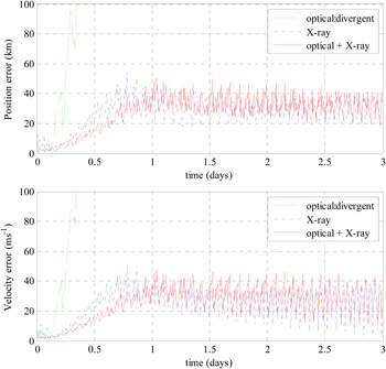
Figure 5. Results of EKF for LMO.
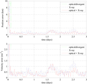
Figure 6. Results of UKF for LMO.
The results of EKF for HMO are given in Figure 7, and the results of UKF for HMO are given in Figure 8. For HMO, the dynamics model is a weak nonlinear system, so both EKF and UKF can achieve perfect navigation. The result of combining optical measurement and X-ray pulsar measurement is obviously better than that of using solely either optical measurement or X-ray pulsar measurement.

Figure 7. Results of EKF for LMO.

Figure 8. Results of UKF for LMO.
Tables 4 and 5 give statistical information of navigation results of LMO and HMO after the filter has converged from the second day.
Table 4. Accuracy comparison of LMO.

Table 5. Accuracy comparison of HMO.

5. CONCLUSIONS
Aiming at a future Mars probe programme, in order to achieve high accuracy of autonomous navigation for Mars probes, an integrated navigation method using single X-ray pulsar measurement and optical data of viewing Martian moons is proposed in this paper.
The simulation results indicate that in the scenarios of both low and high orbits, the autonomous navigation method of Mars probes by combining single TOA of X-ray pulsar measurement and optical data of viewing Martian moons is practicable. The accuracy is better than that of using solely X-ray pulsar measurement or optical measurement.
The autonomous navigation accuracy for LMO can attain a position error less than 1 km (Root Mean Square - RMS) and velocity error less than 0·5 m/s (RMS). For HMO, position error is less than 0·5 km (RMS) and velocity error is less than 0·03 m/s (RMS).
For the low Mars orbit, EKF requires a faster update frequency of observation data, and UKF can achieve perfect navigation with 600 seconds update frequency of observation data. The performance in accuracy of UKF is a little better than that of EKF, but EKF has better performance at time consumption.
ACKNOWLEDGMENTS
This work is supported by the National Natural Science Foundation of China (Grant No.11372150) and the National Basic Research Program of China (973 Program) (2012CB720000).


