


Introduction
The RWV in glaciers is an important parameter for calculating ice thickness and depth of the internal-reflecting horizons (IRHs) from radio-echo sounding (RES) data. In the radar range (1–1000 MHz), the RWV in a glacier depends on many factors, the most important being density, structure and water content of the ice (Reference Bogorodskiy, Bentley and GudmandsenBogorodskiy and others, 1983), and can be noticeably different from the RWV in solid pure ice (e.g. Reference RobinRobin, 1975a; Reference Macheret and ZhuravlevMacheret and Zhuravlev, 1981). Therefore, it is important to obtain field data on the RWV for glaciers having different structures and hydrothermal states. As has been shown in a number of investigations (e.g. Reference Jiracek and BentleyJiracek and Bentley, 1971; Reference Macheret, Zhuravlev and KotlyakovMacheret and Zhuravlev, 1985; Reference Kotlyakov and MacheretKotlyakov and Macheret, 1987), these data can also be used for the calculation of electrical and physical properties of glacier ice.
For the determination of RWV in situ, four basic methods are used: RES in the vicinity of a borehole to bedrock; radio-interferometry and radar logging of a borehole; comparison of the RES and seismic reflection-sounding data; and various modifications of WAR methods (Reference Robin, Evans and BaileyRobin and others, 1969; Reference TrepovTrepov, 1970; Reference DrewryDrewry, 1975; Reference RobinRobin, 1975b; Reference Bogorodskiy, Bentley and GudmandsenBogorodskiy and others, 1983; Reference Jezek and RoelofsJezek and Roellofs, 1983; Reference Macheret, Vasilenko, Gromyko and ZhuravlevMacheret and others, 1984a).
The majority of field data on the RWV have been obtained on the polar ice sheets and cold glaciers using radars operating in the UHF and VHF range. They have been summarized by Reference Bogorodskiy, Bentley and GudmandsenBogorodskiy and others (1983), Reference Jezek, Clough, Bendey and ShabtaieJezek and others (1978) and Reference RobinRobin (1975b). Several measurements have also been carried out on sub-polar glaciers (Reference Ryumin and ZverevRyumin and Zverev, 1969; Reference Zhuravlev, Macheret and BobrovaZhuravlev and others, 1983; Reference EpovEpov, 1984; Reference Macheret, Zhuravlev and KotlyakovMacheret and Zhuravlev, 1985). However, use of this equipment on temperate glaciers, having ice at the melting point and containing a certain amount of water in the interfaces of crystals and in cavities, and in the accumulation areas of a number of sub-polar glaciers with intense summer melting, often becomes ineffective because of the great scattering of radio waves at these wavelengths (Reference Dowdeswell, Drewry, Liestøl and OrheimDowdeswell and others, 1984b; Reference Macheret, Zhuravlev and BobrovaMacheret and others, 1984b; Reference Kotlyakov and MacheretKotlyakov and Macheret, 1987; Reference Vasilenko, Gromyko and MacheretVasilenko and others, 1987; Reference BamberBamber, 1989). Because of this, the best results on such glaciers can be obtained in the HF range (Reference Smith and EvansSmith and Evans, 1972; Reference Watts and EnglandWatts and England, 1976) and a number of HF RWV measurements on temperate glaciers have been done (Reference Blindow and ThyssenBlindow and Thissen, 1986; Reference Jacobel, Anderson and RiouxJacobel and others, 1988; Reference Vasilenko, Gromyko, Dmitriyev and MacheretVasilenko and others, 1988b).
Using HF equipment, RWV measurements were carried out in the summer of 1986 on the temperate Abramov Glacier in the Alai Mountain Ridge (Reference VasilenkoVasilenko and others, 1988a) and in the spring of 1988 and 1989 on two sub-polar glaciers — Fridtjovbreen and Hansbreen on Svalbard (Reference Glazovskiy and MoskalevskiyGlazovskiy and Moskalevskiy, 1989; Reference Glazovskiy, Kolondra, Moskalevskiy and YaniyaGlazovskiy and others, 1991a) (Fig. 1).

Fig. 1. Low-frequency wide-angle reflection (WAR) measurements on Abramov Glacier in the Alai Mountain Ridge (a), Fridtjovbreen (b) and Hansbreen (c) in Spitsbergen. 1 is the glacier boundary, 2 is ice-free land, 3 h the sea, 4 are WAR-measurement sites and their numbers, and 5 are boreholes and their numbers.
A specific peculiarity of Fridtjovbreen and Hansbreen is the presence of an extended IRH at depths from 70 to 180 m (Reference Dowdeswell, Drewry, Liestøl and OrheimDowdeswell and others, 1984a; Reference Macheret, Zhuravlev and BobrovaMacheret and others, 1984b). Other glaciers with extended IRHs are found in Spitsbergen (Reference BamberBamber, 1987, Reference Bamber1989; Reference Macheret, Kotlyakov and SokolovMacheret, 1990; Reference Macheret, Bobrova and SankinaMacheret and others, 1991). Ice-core, borehole and radar studies on Fridtjovbreen (Reference Macheret, Vasilenko, Gromyko and ZhuravlevMacheret and others, 1984a; Reference Kotlyakov and MacheretKotlyakov and Macheret, 1987) showed that these glaciers are a special class of transitional (two-layered) glacier with the upper layer of “dry” cold ice and a lower layer of water-saturated temperate ice. The extended IRH is an indicator of the location of the melting isotherm in such glaciers (Reference Macheret, Zhuravlev and KotlyakovMacheret and Zhuravlev, 1985). The results of the previous determinations of RWV at 620 MHz from ground RES data at borehole 1 (Reference Macheret, Zhuravlev and GromykoMacheret and others, 1980) and from radar logging of borehole 2 (Reference Macheret, Vasilenko, Gromyko and ZhuravlevMacheret and others, 1984a, Reference Macheret, Zagorodnov, Vasilenko, Gromyko and Zhuravlev1985a) (Fig. 1b) showed considerable differences of RWV within the whole glacier sequence and its upper cold layer—161.4 and 172.2 m μ−1, respectively. The lower mean RWV can be caused by the higher wetness of the snow-firn layer during summer measurements at borehole 1. However, there is no satisfactory explanation for the very low RWV equal to 147.7m µs−1, determined from the radar logging data in the upper part (in the interval 117–145 m) of the lower layer of temperate ice. The new RWV measurements on Fridtjovbreen and Hansbreen were carried out just before melting. They can be used to show to what extent such lower RWV are typical for any two-layered glacier. As a whole, the series of investigations on all the above-mentioned glaciers provides the possibility of determining RWV in both cold and temperate ice, and of comparing them with the results of independent measurements on other glaciers.
Characteristics of RWV Measurement Sites
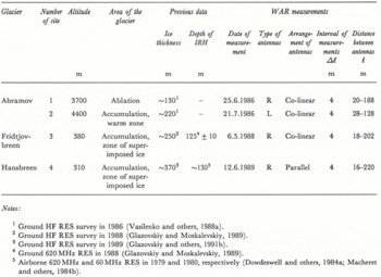
Details on Abramov Glacier, Fridtjovbreen and Hansbreen are given in Table 1. Site 3 on Fridtjovbreen was situated at a distance about 500 m from borehole 2 drilled in 1979 (Fig. 1b). RES and radar logging to a depth of 145 m at a frequency of 620 MHz, as well as temperature measurements and ice-core studies to depths of 115 and 119 m, showed the following (Reference Macheret, Zhuravlev and KotlyakovMacheret and Zhuravlev, 1985; Reference Macheret, Vasilenko, Gromyko and ZhuravlevMacheret and others, 1985b): IRH depth is 120 ± 10m; RWV decreases from 172 to 147.7 m µs−1 and ice temperature rises to the pressure-melting point at depths of more than 117 ± 12 m and 113 m, respectively; and microchannels characteristic of temperate ice were observed in the depth interval 110–116 m. At site 3, the IRH depth was found to be 125 ± 10 m in 1988 by using ground RES data at a frequency of 620 MHz (Reference Glazovskiy and MoskalevskiyGlazovskiy and Moskalevskiy, 1989) confirming the previous airborne and ground RES data at frequencies of 620 and 60 MHz (Reference Dowdeswell, Drewry, Liestøl and OrheimDowdeswell and others, 1984a; Reference Macheret, Zhuravlev and BobrovaMacheret and others, 1984b).
Table 1. Characteristics of measurement sites and the methods of wide-angle reflection on Abramov Glacier, Fridtjovbreen and Hansbreen
Fridtjovbreen has a similar structure in the vicinity of borehole 1 which was drilled in 1975 to bedrock. Reflections from a strong IRH at 620 MHz at a depth of 72 ± 5 m were recorded (Reference Macheret, Zhuravlev and BobrovaMacheret and others, 1984b; Reference Macheret, Zhuravlev and KotlyakovMacheret and Zhuravlev, 1985). A rise in temperature to the pressure-melting point at a depth of about 80 m was recorded, and inflow of liquid water into the borehole was observed between 58 and 81 m. However, the HF RES survey of 1988 did not show the internal reflections at the majority of measurement points on Fridtjovbreen including WAR site 3 and its environs (Reference Glazovskiy, Konstantinova, Macheret, Moskalevskiy, Bobrova and SankinaGlazovskiy and others, 1991b).
On Hansbreen, at site 4 the depth of the IRH according the airborne RES in 1979 at a frequency of 620 MHz (Reference Macheret, Zhuravlev and BobrovaMacheret and others, 1984b) and in 1980 at a frequency of 60 MHz (Reference Dowdeswell, Drewry, Liestøl and OrheimDowdeswell and others, 1984a) is about 130 m. Internal reflections from shallower and greater depths were recorded at the majority of HF RES survey points on Hansbreen in 1989 (Reference Glazovskiy, Kolondra, Moskalevskiy and YaniyaGlazovskiy and others, 1991a). The data from a longitudinal profile crossing site 4 illustrate this peculiarity (Fig. 2). At site 4, the depths of internal HF reflections are 125, 165 and 200 m. Direct exploration of several moulins located at distances of 4–5 km from site 4 was made in the autumn of 1988 and in the spring and autumn of 1989 (Reference SchroederSchroeder, 1990; personal communication from J. Jania and M.Pulina). These show that at depths of 90–120 m there are inclined channels 5–20 m high and 1–5 m wide with several ledges and water pools of meter scale. Thus, the depths of the internal HF reflections and of the IRH are very similar to the upper boundary of this zone, with water inclusions inside the glacier.

Fig. 2. Longitudinal profile of Hansbreen from data of ground low-frequency radio-echo sounding (HF RES). 1 are glacier-surface and measurement points of ground HF RES survey in 1989 (Reference Glazovskiy, Kolondra, Moskalevskiy and YaniyaGlazovskiy and others, 1991a); 2 and 3 are correspondingly the bottom and internal reflections from the same data; 4 are data of HF wide-angle reflection measurements at site 4 in 1989 (see Tables 2 and 3): R and R′ are the lower and upper internal reflection boundaries, Β is glacier bottom; 5 is internal-reflection horizon (IRH) from data of airborne RES at 620 MHZ in 1979 (Reference Macheret, Zhuravlev and BobrovaMacheret and others, 1984b) and at 60 MHz in 1980 (Reference Dowdeswell, Drewry, Liestøl and OrheimDowdeswell and others, 1984a).
Equipment and RWV Measurement Method
A monopulse HF radar (MP 1-8) with shock excitation of the aerials developed at Mary Polytechnic Institute was used for the measurements (Reference Vasilenko, Gromyko, Dmitriyev and MacheretVasilenko and others, 1988b). The transmitted signal spectrum is 2–13 MHz, the central frequency is 8 MHz and the pulse power is 13 kW. Active and reactively loaded dipoles (R- and L-antennas) 16 m and 28 m long, respectively, served as transmitting and receiving antennas.
The common midpoint (CMP) method was used for RWV measurements, i.e. the transmitted and receiving antennas were moved away with a certain interval Δl at equal distance l/2 with respect to the fixed centre of the antenna arrangement. In this case, the influence of the bed inclination on the accuracy of determination of the mean RWV is small, because radio-wave reflection occurs approximately at the same point on the glacier bed.
Type and arrangement of antennas, and values of Δl and l for the measurement sites, are given in Table 1.
Recording of returns on all sites was made by photographing the screen of an oscilloscope. Scanning speed was calibrated with the aid of a quartz signal generator with a time repetition of 0.2 μs. Autotriggering was carried out with direct waves radiated by the transmitting antenna.
The Results of RWV Measurements
Some examples of records obtained on Abramov Glacier at sites 1 and 2 are given in Figure 3a and b. Two groups of regular signals can be distinguished easily: signals A and Ν propagated directly from the transmitting to the receiving antenna, one through air and the other within the near-surface glacier sequence; and returns Β from the glacier bed. In addition, at some antenna separations, there are signals I due to reflections from the glacier surface and/or internal inhomogeneities. At site 1, signals A and Ν are observed separately at distances between antennas l > 28 m; at site 2, with l > 44 m. At shorter distances these interfere with each other forming signals A + N. At site 1, returns from the glacier bed are observed at l ≤ 168 m; at site 2, at l ≤ 128 m. At greater distances their amplitude at site 1 becomes comparable with the noise.

Fig. 3. Examples of radio-oscillograms obtained by low-frequency wide-angle refection measurements on Abramov Glacier at sites 1a and 2b, on Fridtjovbreen at site 3c, and Hansbreen at site 4d. A and Ν are correspondingly signals propagating from the transmitting to the receiving antenna, one through air and the other within the near-glacier sequence; A + N is interference of signals A and N; Β is bottom return; R and R′ are signals from internal-refelction boundaries; I is signal from near-surface and/or internal inhomogeneities.
On Fridtjovbreen and Hansbreen (sites 3 and 4), the bottom signals Β were observed at a greater distance between antennas — up to 202 and 220 m, respectively (Fig. 3c and d), which indicates their lower total attenuation during propagation and reflection as compared with site 1 on Abramov Glacier. In addition, on Hansbreen at site 4 and l ≤ 220 m, unambiguous signals R from an internal interface were detected and less clearly signals R′ from a deeper internal interface were distinguished.
For a simple two-dimensional model of a glacier as a homogeneous isotropic ice layer with a plane interface, the full delay time of bottom returns Β in the approximation of geometrical optics using the CMP method is (Reference GurvichGurvich, 1975):
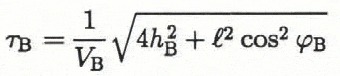
where τB = τd + τ0, τ0, τd is the delay time of the bottom signal Β measured relative to the signal A, τ0 = c/l is the propagation time in air of signal A from the transmitter, c is the RWV in air, VB is the mean velocity of the bottom signal B, h B is the echo depth of the bottom and ϕB is the difference in slope angles of the glacier surface and the glacier bed (subject to their sign). ϕB was determined from geodetic surveys and RES data in the vicinity of the WAR sites.
Equation (1) can be transformed to a linear form
by squaring and assigning

A least-squares procedure may easily be used to find the values of V B and h B:
The velocity of signals N, R and R′ and the echo depth of their penetration into the glacier can be found in an analogous way.
The results of WAR measurements at sites 1, 2, 3 and 4 are shown in Figures 4 and 5 in the form of the regression τ2 = f(2). From these figures, it is seen that the results are almost linear except at smaller l 2. This phenomenon can be explained by the following two reasons. For signals B, the decrease of delay time in the initial parts of graphs τ = f(l 2) results mainly from interference of signals A and N. For site 1, the interference takes place at l ≤ 28 m, at site 2 at l ≤ 36 m, at site 3 at l ≤ 18 m and at site 4 at l ≤ 104 m. The wider area of interference at site 4 results from the parallel alignment of antennas. For signals R and R′ at site 4, the delay time in the initial part of the graph at l ≤ 54 m, on the contrary, increases (Fig. 5b). This can be explained by the apparent dependence of the reflecting boundary depth on the angle of radio-wave incidence, i.e. on distance l between the antennas, and probably results from the smooth change of dielectric permittivity of glacier ice through the depth of the glacier which occurs because of the presence of water-filled cavities. These peculiarities in the initial parts of graphs τ2 = f(l 2) were often observed during WAR measurements on glaciers both in the Arctic and Antarctic (Reference FedorovFedorov, 1978; Reference Bogorodskiy, Bentley and GudmandsenBogorodskiy and others, 1983). For this reason, low abscissa values were excluded from further processing using the least-squares procedure.

Fig. 4. Graphs of delay-time y = τ2 dependence of signals on the distance x = l2 between antennas, obtained during wide-angle refection measurements on Abramov Glacier at sites 1a and 2b for signals Ν propagating within the near-surface glacier sequence and for bottom signals B.
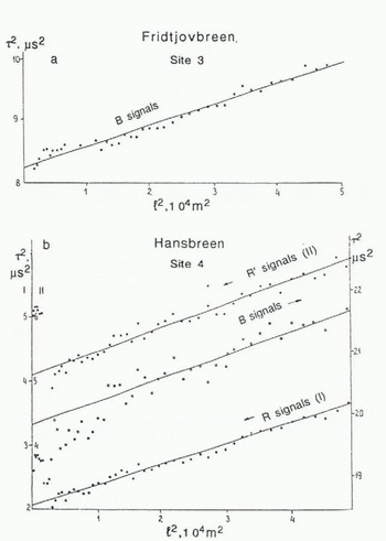
Fig. 5. Graphs of delay-time y = τ2 dependence of signals on the distance x = l2 between antennas, obtained during wide-angle reflection measurements on Fridtjovbreen at site 3 (a) for bottom signals Β on Hansbreen at site 4 (b) for bottom signals B, and for signals R and R’ from internal-reflection boundaries.
The results of processing WAR data at sites 1, 2, 3 and 4 for signals N, R and R′ using Equation (1)–(5)are given in Table 2. For these signals we assume ϕN = ϕR = ϕR′
Table 2. The results of processing data of wide-angle reflection measurements on Abramov Glacier, Fridtjovbreen and Hansbreen

Discussion of the Results
Radio-Wave Velocity–Depth Profiles of Glaciers
On the tongue of Abramov Glacier (site 1), velocities of signals Ν and Β do not differ significantly from each other (Table 2), although the directions and depths of propagation of these signals into the glacier are different. Thus, in the ablation area, the RWV does not change through the glacier depth, and the average RWV is 160.3 ± 1.0 m µs−1. However, it is still not clear why the depth of penetration into the glacier of signals Ν equals 13.8m instead of zero for a direct wave through the ice.
In the accumulation area of Abramov Glacier (site 2), the velocities of signals Ν and Β differ from each other because of the presence of a firn layer. The velocity of signals Ν (V N = 182.3 ± 1.6m μs−1) is close to the average velocity of broad-band (4–330 MHz) electromagnetic signals in the nearby snowpack of about 190 m μs−1 signals in the nearby snowpack of about 190m μs−1 (Reference Gromyko, Vasilenko, Macheret and MoskalevskiyGromyko and others, 1989). Pit data showed that thickness of the snow–firn layer near site 2 exceeds 25 m (Reference Krenke and SuslovKrenke and Suslov, 1980), which agrees with the result that the depth of penetration of signals Ν into the glacier h N = 32.5 m. Taking this into account, the velocity–depth section of Abramov Glacier at this site can be considered as two-layered.
According to the results from both the ground RES and the radar logging of the nearby borehole 2 (see Fig. 1b) at 620 MHz, the velocity–depth section of Fridtjovbreen at site 3 can also be considered as two-layered: velocity V 1, in the upper layer of cold ice, is equal to 172.2 m μs−1 and the thickness of this layer h 1 is 125 ± 10m.
For Hansbreen, two models were considered: two-layered (1) and three-layered (2) (Fig. 6). In the latter case, the less prominent and deeper internal signal R’ was taken into account.

Fig. 6. Velocity-depth section of Hansbreen at site 4 of wide-angle reflection measurements for two-layered model 1 (a) and three-layered model 2 (b). A is “dry” cold ice, Β is water-saturated temperate ice, C is intermediate layer in temperate ice. S and Β are correspondingly surface and bottom of glacier, R and Κ are internal-reflection boundaries.
Assuming absence of radio-wave refraction at the boundary of englacial layers, the velocity V 2 in the underlying layer corresponding to the snow–firn layer at site 2 and the internal reflecting boundaries at sites 3 and 4 can be calculated as

The equation for the velocity V 2′ in the ice layer underlying the internal boundary at site 4 can be calculated as

and the velocity V 1–2 in the intermediate layer 1–2 (between boundaries R and R′ at site 4) is equal to

where h = h B, V M = V B, h 1 = h K, V 1 = V k (K = N, R), h′ 1 = h R′, V′ 1 = V R′.
The results of calculations of velocities V 2, V′ 2 and V 1–2 by Equation (6) are given in Table 3 as corresponding velocity-depth sections. The errors in determining V B, V R and V R′ by a least-squares procedure and Equation (1)–(5) were taken into account.
Table 3. Velocity–depth sections of Abramov Glacier, Fridtjovbreen and Hansbreen from the data from wide-angle reflection measurements and physical characteristics of the glacier sequence estimated from these data

In media with weak absorption such as pure ice, air and water, dispersion within the RES range is negligible, i.e.

where ϵ is the real part of the complex dielectric permittivity of the medium. This makes it possible to compare data from field RWV measurements at different frequencies in other glaciers and data from laboratory measurements of ϵ (Fig. 7).

Fig. 7. Comparison of field-measurement data on radio-wave velocities V in glaciers (a) and laboratory-measurement data of dielectric permittivity ϵ of glacier ice (b). From Reference Bogorodskiy, Bentley and GudmandsenBogorodskiy and others (1983, Table 3), with some changes and additions. Methods and regions of measurements:
-
I. Radio-interferometry of borehole: 1. Canadian Arctic Archipelago, Devon Ice Cap (Reference RobinRobin, 1975b).
-
II. Radio-echo sounding near a borehole drilled to bedrock: 2. Greenland, Camp Century station (Reference Bogorodskiy, Bentley and GudmandsenBogorodskiy and others, 1983; G.de Q. Robin’s data); 3. Antarctica, Byrd Station (Reference DrewryDrewry, 1975); 4, 5 and 6. Sevemaya Zjemlya, Vavilov Glacier (Reference Bogorodskiy, Bentley and GudmandsenBogorodskiy and others, 1983); 7. Tien Shan, Karabatkak Glacier (Reference Ryumin and ZverevRyumin and tyerev, 1969); 8 and 9. Spitsbergen: Fridtjovbreen, borehole 1 (see Fig. lb) (Reference Macheret, Zhuravlev and GromykoMacheret and others, 1980) and Bertilbreen (Reference Zhuravlev, Macheret and BobrovaZhuravlev and others, 1983).
-
III. Wide-angle reflection measurements on ground glaciers: 10 and 11. Greenland, Tuto East station (Reference Robin, Evans and BaileyRobin and others, 1969) and Camp Century station (Reference Bogorodskiy, Bentley and GudmandsenBogorodskiy and others, 1983); 12. Baffin Island, Barnes Ice Cap (Reference Clough and BentleyClough and Bentley, 1970); 13. Sevemaya Zemlya, Vavilov Glacier (Reference FedorovFedorov, 1978); 14. Tien Shan, Tuyuksu Glacier (Reference EpovEpov, 1984) ; 15–19. Antarctica: Roosevelt Island (15) (Reference Jiracek and BentleyJiracek and Bentley, 1971; Reference Jezek, Clough, Bendey and ShabtaieJezek and others, 1978), Dronning Maud Land, station 840 (16, 17) (Reference Clough and BentleyClough and Bentley, 1970), Dome C (18) (Reference Bogorodskiy, Bentley and GudmandsenBogorodskiy and others, 1983); F, Reference Fitzgerald and ParenFitzgerald and Paren (1975); Ρ, Reference Paren and GlenParen and Glen (1978).
-
Continuous lines show the errors of field measurements of radio-wave velocity with correction because of density change in the near-surface snow-firn layer; dotted lines show errors without this correction. The symbol × marks the velocity in temperate ice.
Analysis of Table 3 and Figure 7 shows that the mean velocities V m through the whole ice sequence of two-layered glaciers that have been investigated are higher than in the temperate Abramov Glacier, but are lower than on the majority of cold ice sheets and glaciers where there are data from field measurements in the range 30– 620 MHz. On Hansbreen, the velocity V 2 in the lower layer is close to the mean velocity V m in the temperate Abramov Glacier but lower than on Fridtjovbreen. This can be explained by the presence of an intermediate layer on Hansbreen at site 4 (layer 1–2 in model (2); see Fig. 6b and Table 3) c. 60 m thick with a lower velocity V 1–2 = 145.5 ± 5.5m µs−1. This layer is at depths between 127 and 187 m. It should be mentioned that a similar value of velocity Vʺ 2 = 147.7 m µs−1 was obtained in the upper part of the lower layer 2 on Fridtjovbreen from data of the radar logging of borehole 2 in the summer of 1979 within the depth interval 117–145 m at 620 MHz (Reference Macheret, Vasilenko, Gromyko and ZhuravlevMacheret and others, 1984a; Reference Kotlyakov and MacheretKotlyakov and Macheret, 1987).
Data from the 1989 survey (Fig. 2) give additional information concerning the location of the intermediate layer on Hansbreen. These show that internal reflections can be traced along almost all of the entire longitudinal profile at depths from 100–160 to 160–320 m. Assuming that the shallowest and deepest internal reflections shown in Figure 2 have the same nature as reflected signals R and R’ at site 4, the thickness of this layer is 60–220 m. The presence of only a single extended IRH, i.e. internal reflections from the upper boundary of the intermediate layer, can be explained by strong scattering of radio waves at these frequencies within this layer.
The data in Figure 7 indicate great variability of RWV in cold glaciers. Also, the majority of field measurements give values V higher (ϵ lower) than the laboratory measurements. This is especially noticeable in measurements on ice shelves, but the cause of such differences has not yet been determined (Reference Bogorodskiy, Bentley and GudmandsenBogorodskiy and others, 1983). The most reliable lower limit of RWV in cold ice is 167.7 ± 0.3m µs−1 and comes from radio-interferometry measurements in a borehole on the Devon Ice Cap at about 425 MHz (Reference RobinRobin, 1975b). This corresponds to a value of ϵ = 3.20 ±0.1.
Figure 7 shows that mean velocities V m ≳ 167 m µs−1 are characteristic of cold glaciers. Mean velocities V m ≳ 167 µs−1 are typical of temperate glaciers. On two-layered glaciers, velocities V 1 in the upper layer (negative temperatures) are higher than velocities V 2 in the lower layer, where temperatures are close to or equal to the pressure-melting point. However, as measurements on Fridtjovbreen near borehole 1 show, during the melting period mean velocity V m in two-layered glaciers can increase to the values characteristic of temperate glaciers.
All these data indicate the high sensitivity of RWV to even small amounts of water in the glacier sequence and, on the basis of the magnitude and character of velocity changes with depth, support the idea of classifying glaciers according to their hydrothermal state, i.e. of identifying cold, temperate and transitional (two-layered) parts of glaciers. Also, Equation (7) makes it possible to use data from RWV measurements to estimate physical parameters of the glacier sequence by applying theoretical or empirical dependences of the dielectric permittivity ϵ on density; wetness and structure of glacier ice, firn and snow; content and geometry of various inclusions and impurities, and their distribution as described by Reference Beek, van and BirksBeek (1967) and Reference Bogorodskiy, Bentley and GudmandsenBogorodskiy and others (1983).
In the subsequent analysis of the data obtained, we confine ourselves to considering such important para-meters as the mean density and average water content.
Estimation of Physical Parameters of the Glacier Sequence from Radio-Wave Velocity Measurements
Analysis of deep ice cores from the temperate Amundsenisen and the two-layered Fridtjovbreen (Reference Zagorodnov and ZotikovZagorodnov and Zotikov, 1981; Reference Zagorodnov, Archipov and MacheretZagorodnov and others, 1985) and of speleological studies within several Spitsbergen glaciers (Reference SchroederSchroeder, 1990; personal communication from J. Jania and M. Pulina) has shown that water inclusions are concentrated in channels and cavities of different orientation and size. These inclusions may be approximated as both spherical and randomly distributed linear bodies. Air inclusions can also be considered as bodies of the same form. Therefore, for a quantitative description of the dependence of dielectric permittivity ϵ of dry and wet ice and firn of density ρ and water content W, we assume that these media are two-component heterogeneous mixtures, in which the size of inclusions is much less than the wavelength λ of the radar, and use the simple formulas given by Reference Smith and EvansSmith and Evans (1972) and Reference Robin, Evans and BaileyRobin and others (1969) which are valid for these two limiting cases.
In the first case, the Looyenga mixture formula (Reference LooyengaLooyenga, 1965), which is valid for large concentrations of spherical air and water inclusions in ice, is applied:


where subscripts d, s, i and w denote correspondingly dry and wet glacier ice or firn, dry solid ice (ρi = 917 kg m−3) and water by volume, and θ = ρd/ρi (1 − θ) × 100 – W is water content expressed as a percentage. If ρd > 300 kg m−3, a good approximation of Equation (8) and laboratory measurement data for e is given by the empirical formula of Reference Robin, Evans and BaileyRobin and others (1969) (see Reference Bogorodskiy, Bentley and GudmandsenBogorodskiy and others, 1983):
In the second case, when water inclusions are distributed randomly throughout the ice, Paren’s mixture formula (see Reference Smith and EvansSmith and Evans, 1972) is used:

It follows from Equation (8) and (9) that


and from Equation (10) and (11) that


where V d and V s are velocities corresponding to cold and temperate ice masses. When used with the data given above, we assume ϵi = 3.2 and ϵw – 86.
Average Density of Cold Ice
This parameter can be estimated directly from Equation (12) and (14) using the measured value of V d. The results of this calculation of ρ i for the upper layer of cold ice on Fridtjovbreen and Hansbreen (sites 3 and 4) are given in Table 3.
Direct measurements of the ice-core density from borehole 2 to a depth of 119 m on Fridtjovbreen give an average integral ice density ρ d = 904 kg m–3 (Reference Macheret, Zagorodnov, Vasilenko, Gromyko and ZhuravlevMacheret and others, 1985a). This implies an error in the estimation of density ρ 1 of layer 1 (Fig. 6a) by Equation (13) and (15) of +37 and + 31 kg m−3. Use of the same value pd for Hansbreen (site 4) gives a lower value of ρ 1.
Water Content
For estimating water content in wet firn and ice from Equation (12) and (14), it is necessary to know the average density ρ d of dry firn and ice.
On Abramov Glacier, a study of the ice core at site 1 from the depth interval of 31.6–105.6 m gives ρ d = 908 kg m−3 (Reference Krenke and SuslovKrenke and Suslov, 1980). At site 2, taking into account snow-pit density measurements to a depth of 13.2m (Reference Krenke and SuslovKrenke and Suslov, 1980). At site 2 taking into account snow-pit density measurements to a depth of 13.2m (Reference Krenke and SuslovKrenke and Suslov, 1980) and further assuming a smooth increase in density with depth to a value of 908 kg m −3, the average densities of the whole snow-firn and glacier sequence are correspondingly 734 and 882 kg m−−3.
Investigations of the ice core from borehole 2 on Fridtjovbreen showed that the dependence of ice density on depth z is described by a function ρ(z) = 879.5z 0.0072 (Reference Macheret, Zhuravlev and KotlyakovMacheret and Zhuravlev, 1985), from which average ice density in the lower ice layer is equal to 912 kg m−3. The same density value can also be assumed for the lower ice layer on Hansbreen at site 4.
The above-mentioned values for firn and ice density ρ d and the data of Table 2 were used to estimate mean water content W in temperate firn and ice layers on Abramov Glacier, Fridtjovbreen and Hansbreen. The results of the calculations are given in Table 3. These show that estimated water content in the temperate ice of Abramov Glacier differs in both cases by more than 0.55% and is close to the results given by thermal-balance measurements on this glacier where this value is about 2% (Reference Krenke and SuslovKrenke and Suslov, 1980). The greatest difference between these equations is for the intermediate layer 1–2 on Hansbreen (site 4).
Variations of Water Content in Glaciers
From Table 3 it can be seen that estimations of W in Abramov Glacier and in the lower layer of Fridtjovbreen and Hansbreen obtained here agree well with the present ideas of water content in temperate glaciers from 0.1 % up to 1–2% (Reference GolubevGolubev, 1976). The exception is the intermediate layer 1–2 on Hansbreen at site 4 where an anomalously high value of W was estimated at about 4–5%. The most probable cause of this is the existence of cavities and channels within the glacier ice with water accumulations remaining during the winter below the boundary between cold and temperate ice, the depth of which, as shown by investigations on Fridtjovbreen (see above), is close to the IRH depth.
Reference BamberBamber (1987) has shown that the IRH level in two-layered glaciers on Spitsbergen is well described by the piezometric surface of Röthlisberger channels (Röthliseason, are hypothesized to be the residues of a large-scale network of conduits which drain the surface meltwaters to one or more channels at depth. Some of these are closed off in the winter and water is trapped in cavities which remain in the ice at the melting-point temperature (Reference BamberBamber, 1988).
The data of airborne RES from 1983 (Reference BamberBamber, 1987, Reference Bamber1989) showed that the power-reflection coefficient (PRC) from IRHs on the two-layered glaciers of Spitsbergen vary from −15 to −30 dB. Using Mie-scattering theory, Reference BamberBamber (1988) showed that such high values of PRC at 60 MHz are consistent with the presence of an ice layer below the IRH containing 1% by volume of spherical water inclusions approximately 0.25 m in radius. Since the size of these water inclusions is much less than the central wavelength of our radar (λ = 37.5m), the intermediate layer 1–2 in model (2) can be considered as consisting of a heterogeneous mixture of ice, air and water with an effective dielectric permittivity ![]() and plane boundaries. The PRC from such a boundary is calculated as
and plane boundaries. The PRC from such a boundary is calculated as

where, from Equation (7), ![]() is the effective dielectric permittivity of the lower part of the upper layer 1 consisting of cold ice with air bubbles and having a thickness of Δh
1 < λice, and Vd1 and V
1–2 are the RWV in the layers.
is the effective dielectric permittivity of the lower part of the upper layer 1 consisting of cold ice with air bubbles and having a thickness of Δh
1 < λice, and Vd1 and V
1–2 are the RWV in the layers.
Using the data in Table 3 for site 4 on Hansbreen and Equation (16), R 1,2 = −20.3 ± 1.2dB. Thus, the calculated value of R 1,2 is close to the average values of PRC from IRHs on two-layered glaciers of Spitsbergen (Reference BamberBamber, 1987, Reference Bamber1989). Deviations of PRC from this value can be connected with variations in the size and content of water inclusions and, consequently, velocities V s in the lower layer of water-saturated ice which, with Equation (16), can be estimated as

assuming that the error of determination of R 1,2 is small. For site 4 on Hansbreen, assuming V d = 176.8 m µs−1 (see Table 3) and R 1,2 = −20 to −30 dB, we get V s = 144.6 to 166.0 m µs−1. The velocities V s are of the same order we obtained during the summer and spring measurements on Fridtjovbreen in borehole 2 and at site 3. However, practical application of Equation (17) for estimating variations in V s (and, consequently, variations of water content) from the data of PRC measurements at higher frequencies is difficult because of the broad range of PRC determinations — about ±5 dB (Reference BamberBamber, 1987, Reference Bamber1989; Reference Macheret and VasilenkoMacheret and Vasilenko, 1988).
It can be supposed that, as on Hansbreen at site 4, similar intermediate layers of water-saturated ice can be present in other Spitsbergen glaciers (Reference Macheret, Kotlyakov and SokolovMacheret, 1990; Reference Macheret, Bobrova and SankinaMacheret and others, 1991), i.e. these glaciers can have more complicated internal structures with an intermediate layer containing an increased content of water inclusions. Specifically, such an intermediate layer, apparently, can be proposed for Werensköldbreen where, during airborne RES in July 1979 and in September 1984, seasonal changes of the character of internal reflections were noticed and a series of reflections having quasi-hyperbolic form was noted and was probably connected with interglacial water accumulations. Short quasi-hyperbolic tracks of internal reflections below the IRH observed in the lower part of Fridtjovbreen (Reference Macheret, Zhuravlev and KotlyakovMacheret and Zhuravlev, 1985) can also be connected with water accumulations in the upper part of the temperate ice layer.
Seasonal and annual variations of water content in the glacier sequence can also be accounted for by the noticeable difference of RWVs in the lower layers of ice on Fridtjovbreen and Hansbreen (see Table 3), as well as for the difference in average velocities V m, measured on Fridtjovbreen at borehole 1 in the summer of 1977 (V m = 161.4m µs−1) (Reference Macheret, Zhuravlev and GromykoMacheret and others, 1980) and at WAR site 3 in the spring of 1988 (V m = 169.6 ± 2.1 m µs−1) (see Table 3).
The above facts make it possible to consider repeated measurements of RWV in glaciers as a perspective for the study of seasonal and annual changes of their hydro-thermal regime and water content. For this purpose, data of repeated PRC measurements from extended internal boundaries and the bottom of two-layered glaciers should be used. The available data on RWVs in two-layered subpolar and temperate glaciers (see Table 3 and Fig. 1 ) also provide a basis to express any views concerning peculiarities of their hydrothermal state and evolution.
The measurements carried out on Vernagtferner in March 1983 (Reference Blindow and ThyssenBlindow and Thyssen, 1986) showed that in the accumulation area the RWV in ice underlying a snow–firn layer c. 20 m thick V 2 = 165 ± 1 m µs−1 and, below the equilibrium line V m = 172 ± 1 m µ−1. These values of velocity are characteristic of temperate ice with a small water content and cold ice, respectively. Thus, Vernagtferner can be considered as polythermal. A noticeable difference in RWVs in the temperate ice of Vernagtferner and Fridtjovbreen, on the one hand, and of Abramov Glacier and Hansbreen, on the other, can be explained by them achieving different stages of evolution. Particularly, on Hansbreen there is a comparatively thick intermediate layer of temperate ice with an anomalously low RWV (V1–2 = 145.5 ± 5.5m µs−1), indicating that Hansbreen has a well-developed internal hydrological drainage system.
Conclusions
Wide-angle reflection measurements on temperate and sub-polar glaciers with records of returns from the bed and internal boundaries using HF monopulse equipment make it possible to measure with an accuracy of about 1% not only average radio-wave velocity and ice thickness but also to determine dielectric characteristics of the glacier sequence and to use them to estimate such important physical parameters as average density and water content. Specifically, on two-layered glaciers, low-i −equency studies make it possible to determine RWVs in he upper cold and lower temperate ice layers, to isolate horizons with different RWVs within the lower layer, as well as to estimate water content in these layers and horizons. In the accumulation areas of glaciers, including a firn zone, this method also makes it possible to estimate analogous parameters and the thickness of the snow-firn layer.
The high sensitivity of RWV, even to a small water content in the glacier sequence, makes it possible to carry out regime observations on the change in water content in different parts of cold, sub-polar and temperate glaciers, and to characterize the hydrothermal state of glaciers or their individual parts.
Acknowledgements
The authors are grateful to Dr A. F. Glazovskiy, Professor M. Pulina, Dr J. Jania and Dr P. Glawacki for considerable help in the field investigations and useful discussions of the results obtained.
The accuracy of references in the text and in this list is the responsibility of the authors, to whom queries should be addressed.


