


1. Introduction
1.1. Unconformable stratigraphy
Unconformities characterize the stratigraphy beneath the large megadune fields of East Antarctica. These fields, covering an estimated 500 000 km2, are particularly preva lent in the Byrd Glacier catchment (Fig. 1). They are characterized by low-amplitude trains of dunes having wavelengths of 2-5 km and amplitudes of 2-8 m (Reference Fahnestock, Scambos, Shuman, Arthern, Winebrenner and KwokFahnestock and others, 2000;Reference Frezzotti, Gandolfi and UrbiniFrezzotti and others, 2002). Ground-penetrating radar (GPR) profiles have revealed that regular series of prograded bedding sequences, known as cosets, 7-12 m thick and up to 10 km long form in the firn beneath these trains (Reference Fahnestock, Shuman, Albert and ScambosFahnestock and others, 2004; Reference Scambos, Fahnestock, Shuman and BauerScambos and others, 2004). Along the traverse shown in Figure 1, Arcone and others (2012;hereafter referred to as Part I) showed that similar but more irregular stratigraphy forms within the firn of the peripheral areas, as well, and contains considerably larger cosets. Here we discuss similar englacial features we imaged to >2 km deep with GPR along the same traverse, and which allow us to generalize this stratigraphy to much of the catchment.
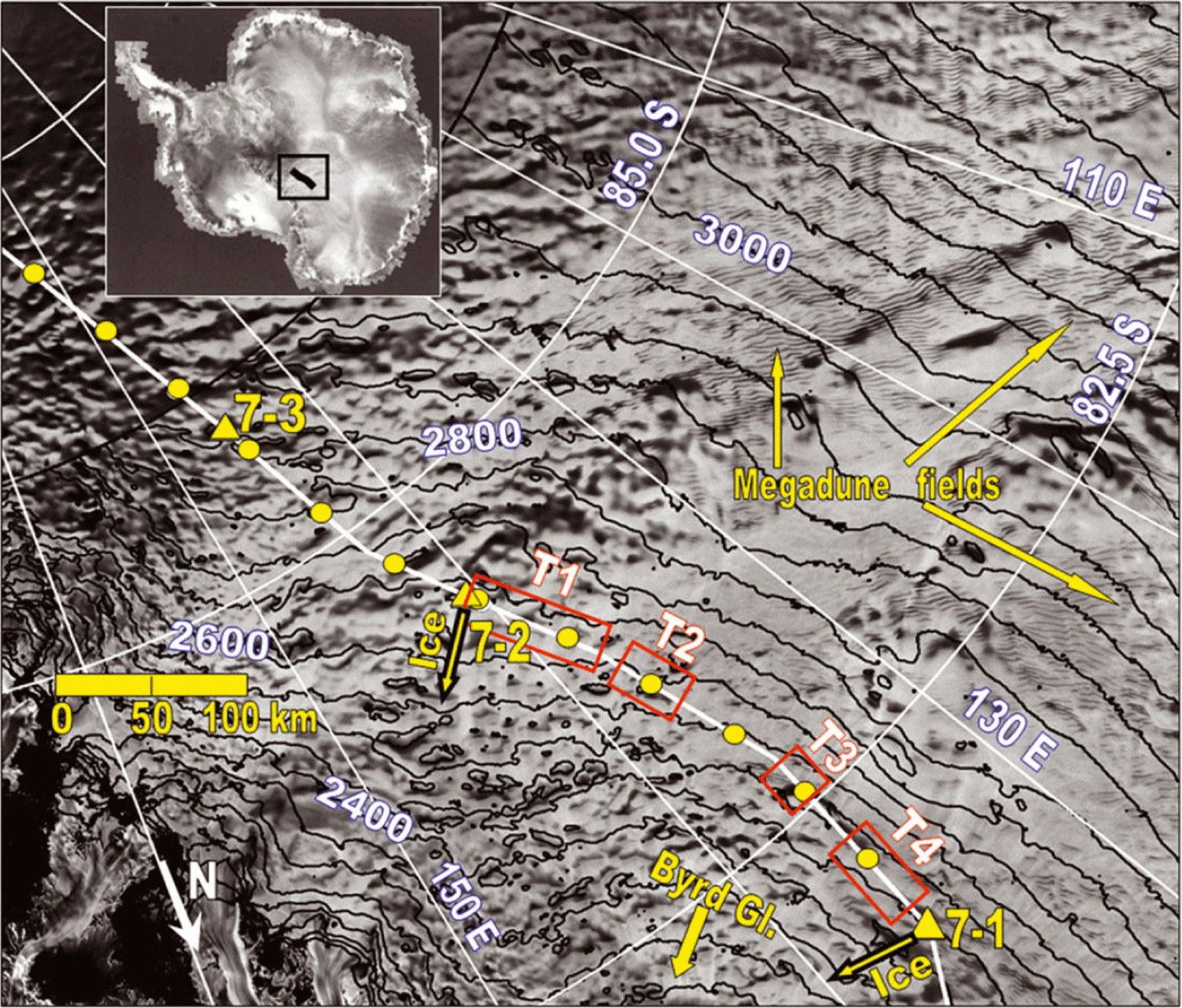
Fig. 1. The 1997 RADARSAT-1 image of part of East Antarctica, with the 2007 US-ITASE II traverse superimposed. Yellow dots along the traverse are 50 km apart. Elevation contours are in 50m increments. The megadune fields appear as dark and light stripes, which indicate windward and leeward slopes, respectively. Peripheral to, and within the fields are sporadic dark-toned areas of accumulation. Unconformable stratigraphy extends _650 km south of site 7-1. The boxes indicate segments T1–T4. Yellow triangles mark sites 7-1, 7-2 and 7-3 where we obtained ice velocities and cores.
As discussed in Part I, in the megadunes environment, accumulation is confined to windward slopes, a process known as antidunal accumulation. This results in cosets, which extend beneath the leeward slopes, and then the next windward slope in the downwind direction. The larger and more irregular cosets we discuss in Part I generate at large windward slopes that appear to be controlled by subglacial relief, so they are stable with respect to bed features. Through modeling we find average accumulation rates along windward slopes as high as 0.16 m w.e. a-1 result from topographic stability, and an unusual ice speed near 30 m a-1. These rates and speed are much higher than estimated regional values. The accumulating and prograding slopes of these cosets, as well as those of megadunes, correlate closely with dark areas we see in a RADARSAT image of the Byrd catchment. The unconformities result from the accumulation hiatus of the wind-glazed leeward slopes. Recrystallization beginning just beneath the glaze forms layers in which the density stratification of the older coset beds appears modified or eliminated. The layers continue to grow both upward and downward after burial, possibly aided by vapor transport (Reference SeveringhausSeveringhaus and others, 2010;Part I).
For 650 km from site 7-1 (Fig. 1) we recorded englacial stratigraphy to the ice bed using a 3.2 MHz GPR (Reference JacobelJacobel and others, 2008, Reference Jacobel, Lapo, Stamp, Youngblood, Welch and Bamber2010;Reference Welch, Jacobel and ArconeWelch and others, 2009). Unconformable horizons appear at depth throughout this segment of the traverse and are typically less than ~30km long, which is similar to the coset lengths found in Part I. The in situ pulse length of 80m for this radar gives a vertical horizon resolution of 40 m (Fig. 2). This resolution is comparable with the thickness of the cosets shown in Part I. Although the 40 m resolution precluded the imaging of thinner coset bedding sequences, along one segment thicker sequences are prominent, some having dimensions that range over 100 m (Reference Welch, Jacobel and ArconeWelch and others, 2009). Thinned by compression at depth, these features evolve from much thicker sequences near the surface. Also important to our interpretation is that 3.2 MHz signals respond primarily to contrasts in conductivity, a, between acidic layers (Reference Moore, Wolff, Clausen and HammerMoore and others, 1992; Reference Hempel, Thyssen, Gundestrup, Clausen and MillerHempel and others, 2000), whereas 200 MHz (and higher) signals respond primarily to density contrasts (Reference Arcone, Spikes, Hamilton and MayewskiArcone and others, 2004, Reference Arcone, Spikes and Hamilton2005a, Reference Arcone, Spikes and Hamiltonb; Part I). This poses the question of whether or not the recrystallization that modified our 200 MHz density strata in firn has modified the acidity strata as well. We explore this question below.
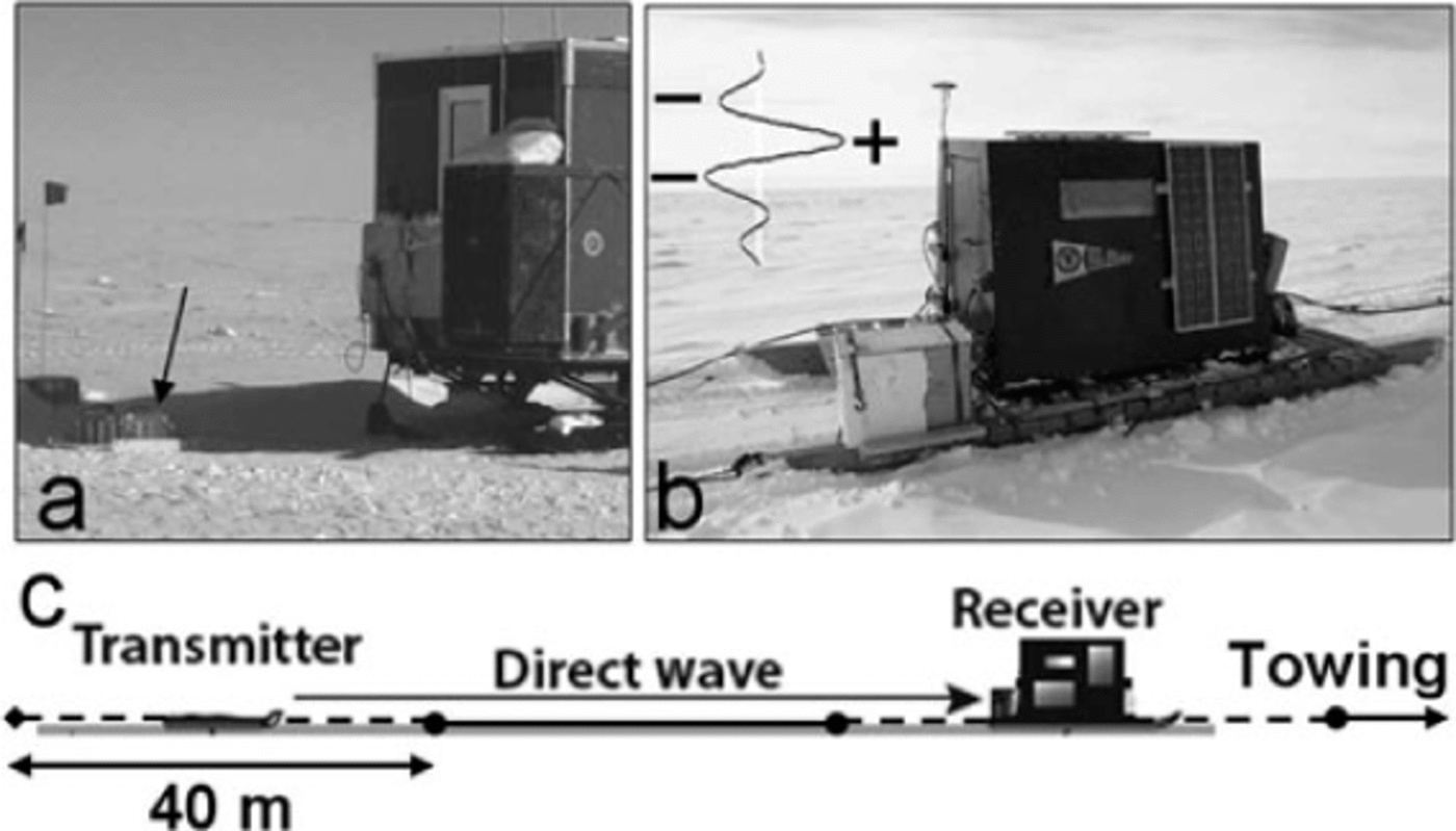
Fig. 2. (a) 200MHz antenna unit on a Teflon sled; (b) St Olaf 3.2 MHz receiver housing; and (c) diagram of the 3.2 MHz system in tow. In (b), the 3.2 MHz pulse waveform is 80m long in ice, which provides 40m of vertical interface resolution. The – + – symbols indicate the phase polarity sequence of the successive halfcycles. In (c) the dashed lines represent the dipole antennas and the arrow labeled ‘Direct wave’ depicts the direct coupling by the 3.2 MHz pulse that masks returns to 135–150m depth.
1.2. Objectives and approach
Here we describe the morphology and dimensions of the deeper englacial cosets and explore how they relate to those we profiled in firn. Our main objective is to determine if the modified firn layers are visible in the englacial profile and if so, why. We consider the resolution limitations of our 3.2 MHz pulse, the waveforms of horizons that appear to delineate the cosets, and compare high- and low-frequency GPR profiles of recrystallized firn to find more evidence of the fate of acidic strata. A second objective is to find if these large and deep cosets are related to present upstream surface features, which would imply their long-term spatial stability, as suggested by our results in Part I. We use previously mapped ice flowlines and the parallel nature of deep stratigraphic folding to argue that these englacial cosets were generated by features identified within RA- DARSAT imagery.
Linking englacial features from one radar profile to the other within the firn regime is not straightforward because of the minimal region of overlap in the depth dimension. We recorded 200MHz profiles from the surface to only 90m depth, while the coverage at 3.2 MHz typically extends from 135-150 m to the bed because direct coupling between the 3.2 MHz antennas masked the stratigraphy above. However, at a compromise in vertical resolution we alleviated the direct coupling with a high-pass filter that created a 10- 20MHz bandwidth multi-cycle signal that enabled us to resolve more of the shallow internal stratigraphy. After applying a normal moveout correction to compensate for the wide antenna separation and correct for horizon dip, we image all but the top 42m. Thus, the 200MHz and the filtered 3.2 MHz GPR profiles overlap from 42 to 90 m. For the typically weak firn values of 10-6 < σ <10-5 Sm-1 (Reference Shabtaie and BentleyShab-taie and Bentley, 1995), an interfacial Fresnel reflection coefficient is proportional to the contrast, A a, between ice layers (Reference Arcone and KreutzArcone and Kreutz, 2009), and inversely proportional to frequency. This means that a typical acidity contrast will be at least 20 dB stronger in the filtered low-frequency data than at 200 MHz and therefore will likely be detectable.
2. Study Site
Figure 1 superimposes part of the 2007 United States International Trans-Antarctic Scientific Expedition (US-ITASE; Reference MayewskiMayewski, 2003) traverse, which includes the segments that we discuss, upon the 1997 RADARSAT mosaic. This part of the traverse crossed the Byrd Glacier catchment (Reference StearnsStearns, 2007) which extends to ~-15km south of site 7-2. The traverse was occasionally near a few megadune features, but at least 130 km from continuous megadune fields. The englacial stratigraphy in this traverse portion is characterized by unconformities for 650 km south of site 7-1. By 750 km south of 7-1 both firn and englacial horizons become continuous and surface-conformable.
The traverse segments are nearly orthogonal to ice flow, with speeds of 86.71 m a-1 (7-1), 30.09 m a-1 (7-2) and 41.47 m a-1 (7-3), measured at an accuracy of about ±5.8 m a-1. These speeds are qualitatively consistent with the balance velocities of Reference Bamber, Gomez-Dans and GriggsBamber and others (2009), and the directions are consistent with flowlines (Reference Liu, Jezek and LiLiu and others, 1999) shown later. The local average surface katabatic wind directions are based on atmospheric modeling (Reference Parish and BromwichParish and Bromwich, 1987;Reference ParishParish, 1988;also shown by Reference Siegert, Hindmarsh and HamiltonSiegert and others, 2003). The wind direction is generally south to north and parallel to our traverse near site 7-2. By 100-150km south of site 7-1 the wind turns towards the Ross Ice Shelf, and at 35° to the northeast. Ice cores to 40-50 m depth obtained at these three sites contain extensive recrystallization, so dating them has not been possible.
3. Methods
3.1. GPR
We describe the 200 MHz system (Fig. 2a), pulse waveform, and processing we used for profiling of firn in Part I. The 1.5- wavelength 200 MHz pulse has a length of 1.4 m in ε = 2.7 firn, which gives a 0.7 m reflection horizon resolution in the vertical dimension.
We constructed our own deep-sounding system (Reference Welch and JacobelWelch and Jacobel, 2003, Reference Welch and Jacobel2005), including resistively loaded dipoles towed collinearly, with each arm 20m long (Fig. 3b and c). The peak amplitude of the pulse spectrum is 3.2 MHz (Fig. 2), which we determined from a subglacial lake reflection farther along the traverse (Reference Welch, Jacobel and ArconeWelch and others, 2009). The −+− amplitude polarity sequence of the waveform appears as black-white-black bands in a profile. This particular waveform characterizes a reflection from an interface between a relatively lower permittivity or conductivity material (e.g. ice) above and a relatively higher material (water, rock, sediments, more conductive ice) below, or from a thin (relative to a wavelength) ice layer embedded in a relatively less conductive ice matrix.

Fig. 3. Segments T3 and T4 (red boxes) superimposed on a RADARSAT image that includes the upstream environment. Elevation contours are in meters, and black dots along the traverse are spaced 50 km. We estimate a±1 km error in aligning the crossing of the flowlines (yellow dashed) across the traverse. We interpret features near labels A, B and C as the origin of similarly labeled features in Figure 4, as discussed in the text. The red-andwhite dashed line along 1208 E separates features B and C, the latter of which resides in a region of relatively stronger convergence, as also indicated by folding in the radar profile. The red stippling indicates areas of plateaus identified in 5m ICESat (Ice, Cloud and land Elevation Satellite) contours. Elevation contours just west of T4 indicate that ice speed accelerated within this short distance to reach 87ma–1 by site 7-1.
The peak radiated power was ˜2.5 kW. After analog-to- digital conversion of the radio-frequency signals, we recorded 8192 14-bit samples per trace at an interval of 5 ns to give a total time range of ˜43 × 103 ns (3.6 km in ice). Each trace was recorded after a 1000-fold stack, which provides 30 dB suppression of random noise. Profile traces are typically recorded every 3-4 m of travel along the surface and are interpolated to a precise 3.5 m separation after distance normalization. We recorded with no range gain, and applied none during processing. We post- processed with high- and low-pass frequency filtering to alleviate noise, and used a two-dimensional Kirchhoff migration to properly place reflection horizons and collapse diffractions.
The direct surface arrival from our free-running transmitter triggered the oscilloscope receiver. In our 3.2 MHz profiles, the top 135-150 m of the firn and ice are masked by the strong direct coupling, which we remove by horizontal filtering to leave only noise to these depths. To compensate for these shallow depths, we simultaneously recorded data in a lower-gain, high-pass filtered (10- 20MHz) channel that alleviates the direct coupling and allows horizons to be imaged within 42 m of the surface, as mentioned above. The wide center-to-center 130 m antenna separation likely provides some, but unknown, distortion of the dip of the shallowest imaged horizons in the range of 42-70 m depth. These higher-frequency profiles are not migrated.
We corrected all profiles for surface elevation. We calibrated depth, d, within the profiles using the simple equation
where c =3 × 10⁸ms-1 and e = 2.7 for firn and 3.15 for ice. We justify this firn value and the likely error in using it in Part I. The englacial depth calibration employs a normal moveout correction using our antenna separation and the ice value of e, which for the 10-20 MHz data provides an estimated depth error of <10% at the shallowest depth of 42 m. We fixed a 500 m depth scale grid on all englacial profiles, depicting values relative to the surface elevation at the left-hand edges. At other locations in the profiles, depths relative to the surface may be displaced by up to 50 m because of changes in the surface elevation across the profile displayed.
We display profiles in a grayscale amplitude format: white indicates positive signal strength, black indicates negative, and gray is near zero. Our englacial 3.2 MHz and firn-englacial 10-20MHz profiles are compiled traces of waveform amplitude. Our firn profiles were additionally processed with a Hilbert magnitude transform, which captured pulse amplitude envelopes and increased horizon clarity. Signal amplitude is then represented with dark tones.
3.2. GPS
We used differential kinematic GPS to determine our traverse position and elevation, with an antenna mounted on the traverse vehicle that dragged our 200 MHz radar antenna. Our accuracy for the GPS antenna location is better than 0.2 m for elevation and better than 0.1 m for horizontal position, based on root-mean-square values. GPS antenna elevation is corrected for its height above the GPR antennas. The 200 MHz antenna unit was 8.5 m behind the GPS antenna. The midpoint between the two 3.2 MHz antennas was ˜143.5 m behind the GPS antenna. We correct for the 135 m displacement between our 200 MHz and lower-frequency profiles, but any misalignment of this order is insignificant given the 30-50 km scale of our profiles. We measured ice velocity by determining kinematic solutions to 4-20 hours of dual-frequency GPS data each day, with surveys at each site performed at least 1 day apart. Position uncertainty is 8 mm, which corresponds to an error in annually averaged speeds of about ±5.9 m a-1 and places the error percentage between 7% and 20% over the range of speeds (87-30 m a1, respectively) we measured.
3.3. Satellite imagery
We show both 2006 MODIS (Moderate Resolution Imaging Spectroradiometer;620-876 nm wavelengths, 250 m resolution) and 1997 RADARSAT-1 (6 cm wavelength, 125 m pixel resolution;Reference Liu, Jezek, Li and ZhaoLiu and others, 2001;Reference JezekJezek, 2003) satellite- based images to give the surficial context of the environment along and far up-ice of our traverse. Windward slopes generally appear dark in RADARSAT images and light in MODIS images, with the corresponding opposite tonality on leeward slopes. MODIS images best reveal megadunes, while RADARSAT images also show megadunes but best reveal larger and isolated accumulation features in dark tones. The causes of the different tonalities are discussed by Reference Fahnestock, Scambos, Shuman, Arthern, Winebrenner and KwokFahnestock and others (2000) and in Part I.
4. Results: Cosets and Modified Layers
4.1. T4: resolved englacial cosets and folding
Figure 3 shows a RADARSAT image depicting the segment of T4 we discuss and the environment further up the flank of the ice sheet. This segment is 17-67 km from site 7-1. The 87 m a-1 ice speed at site 7-1 is directed nearly orthogonal to T4. The modeled katabatic wind is ˜35° east of north. The converging ice flowlines of Reference Liu, Jezek and LiLiu and others (1999) cross at about 10-30 km further south. Along these flowlines, Reference Bamber, Gomez-Dans and GriggsBamber and others (2009) indicate anomalous balance speeds in this tributary feeding Byrd Glacier, grading from about 5 m a-1 250 km to the west of T4, to 20-30 m a-1 along T4. These are higher flow speeds than for surrounding areas, but still considerably less than our measured value of 87 m a-1 at site 7-1. The RADARSAT image shows that megadune fields and large dark accumulation features lie farther to the west up the flank of the ice sheet.
Figure 4 shows the 3.2 MHz profile for this segment. Flow is mainly into the page. The englacial stratigraphy is visible from about 150 to 2400 m depth. The ice-bed horizon contains no special features and is mainly characterized by the simple waveform shown in Figure 2. In general, there are two kinds of englacial horizons in this segment. The first are the major, mainly horizontal (considering the 10x vertical exaggeration) horizons. They last <20 km before merging with another similar major horizon, and occur to nearly 2500 m depth throughout the record. Many exhibit the same waveform polarity sequence as does the bottom horizon (indicated by small arrows in Fig. 4). The second kind (boxes in Fig. 4) are the bedding horizons, which are unconformable with the major horizons that delineate them. These packages of bedding sequences are cosets, and their reflection horizons are responses to acidic strata. The thicknesses of these cosets are obviously enhanced by the transverse compression evidenced by folding below ˜800 m depth. By analogy with our firn results in Part I, the major horizons are likely responses to a density-modified and recrystallized layer between two sequences. The leading edges, therefore, delineate entire cosets. We discuss their likely relative conductivity below.

Fig. 4. 3.2MHz profile of segment T4. Flow is mainly into the page. The depth scale here and in Figure 5 is with respect to the top of the noise band. Label A refers to the speckle features, labels B and C indicate cosets and label D indicates unstratified features. The general folding begins at _800m depth, and separates features B and C. It is often parallel and does not correspond with the subglacial relief. Stratification disappears within 500m of the bottom. The detail of B* shows two sigmoidal beds and evidence of an intervening horizon. The unmigrated detail of D* shows a waveform indicative of a higher conductivity within the unstratified layer. The yellow arrows indicate prominent horizons with the same waveform polarity.
Figure 4 shows labels just below several features. Labels A are below layers of speckle, 40-60 m thick. The speckle patterns are likely responses to bedding sequences, the thicknesses of which are insufficient to be well resolved by our pulse. These layers occur to ˜-600m depth from 17 to 32 km, decrease to ˜400 m depth from 32 to 52 km and then deepen to ˜600m depth on the south side.
Labels B refer to the 5-15 km long cosets from 400 to 800 m depth. Their upper delineating horizons dip to the north, while the 2-3 km long bedding planes dip to the south. Some sigmoidal bedding horizons appear to span 250 m thickness (Fig. 4, inset), but they are crossed by intermediate and more horizontally disposed horizons, such as those in the inset. Changes in bedding horizon curvature across an intermediate horizon in this inset suggest that this is an image of adjoining sequences from two different cosets, each with a maximum sequence thickness less than 150 m.
Labels C indicate the thickest cosets and are at 8001500 m depth. They are up to 8 km long, with most bedding 2-3 km long that dips south. Their folded, synformal appearance, thickness and starting depth of ˜800m distinguish cosets C from cosets B. In the detail in Figure 5a, most of coset C*, from 40 to 44 km, shows no consistent evidence for any cross-cutting horizons, and mostly distinct upper and lower delineating horizons, outlined in red. Consequently, C* appears to be a single coset. As a result of folding, the maximum C* sequence thickness of 150m in a direction normal to the bedding horizons becomes 210 m in the vertical direction, including the thickness of the upper delineating horizon. A 150 m thickness is much greater than the 90 m we observed for firn cosets in Part I, but is possible because acidic beds, as opposed to density layers, will not extinguish as they deepen into the englacial regime, just as they do in regions of conformable stratigraphy.
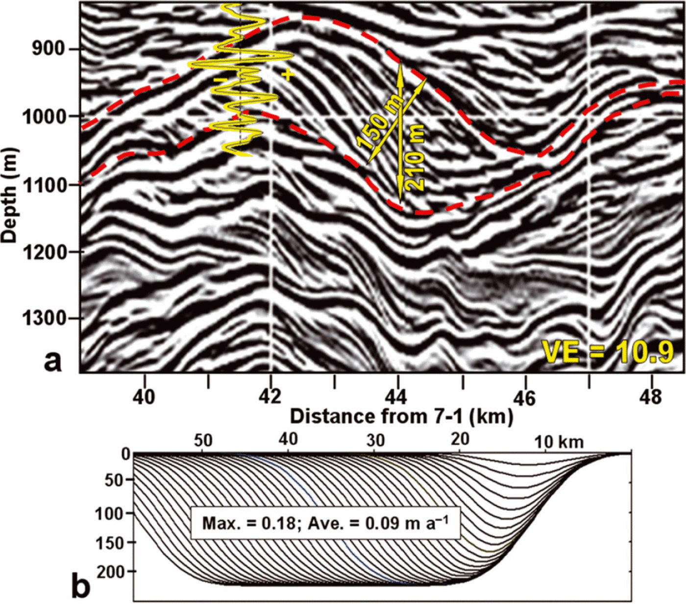
Fig. 5. (a) Coset C* from Figure 4, and (b) surface model of an axial section without topographic correction, assuming that the radar profile is a transverse section. The dashes in (a) outline our interpreted delineation of this coset, and the polarity sequences of the superposed waveform show that the upper and lower delineating horizons are of relatively higher conductivity. The model in (b) is based on a constant water-equivalent accumulation rate, the maximum and the windward slope average of which are labeled. Each model contour represents 100 years of accumulation.
The D features in Figure 4 are 3-8 km long, occur below 1200 m depth and reach 160 m thickness at about 1100m above the bed. The similarity of their folded shapes, thicknesses and lengths to those of cosets C suggests they are cosets. However, they contain no internal bedding horizons that do not conform with their delineating horizons. Instead, they contain weak horizons that conform with the horizons above, which means that these internal horizons are multiple reflections generated in an overriding layer. The detail of feature D* in the Figure 4 inset is unmigrated data, and so precludes any removal of bedding horizons by the migration process. Therefore, these features must have acidic bedding layers that are too thin to resolve;these, along with the waveform in the inset, are discussed below.
Figure 4 reveals that stratigraphic folding begins below ˜800 m depth. Much of the folding appears parallel (Reference BillingsBillings, 1972;Reference SuppeSuppe, 1985;Reference RobertsRoberts, 1989) wherein horizons generally maintain their vertical separation for several kilometers, such as from 47 to 51 km at 1000-2000 m depth. In addition, folding from 39 to 57 km is harmonic, whereby the form of the folds generally repeats with depth. In the detail of Figure 5a the dipping upper and lower delineating horizons of C* (indicated with dashes) and of two deeper and major horizons are nearly parallel between 42 and 45 km. In other places, nonparallel folding occurs, such as from 51 to 52 km (Fig. 4) where the dips of some fold limbs steepen and lengthen with depth below 1000 m, and plunge nearly 400m. The association of this folding with converging flow implies that the folding is transverse to the flow and so the hinge lines are parallel to the flow.
4.2. T1: unresolved englacial cosets and folding
The T1 segment spans 71 km and ends at site 7-2 (Fig. 6). Ice flow is nearly orthogonal to the traverse at site 7-2, where we measured velocity at 30.09 m a-1 directed 58° east of north. Megadunes appear in the RADARSAT image ˜-80km west of the northern end of T1, and there is an extensive megadune field another 50 km further west. Several tributary flowlines that converge toward Byrd Glacier (Reference Liu, Jezek and LiLiu and others, 1999) cross T1 and are consistent with the balance-velocity stream mapped by Reference Bamber, Gomez-Dans and GriggsBamber and others (2009). Their map shows velocities near site 7-2 similar to our value. The inset in Figure 6 shows the accumulation feature surrounding 7-2. The elevation increases only 33 m from north to south along this segment, while the ice-bed elevation decreases nearly 1000 m from -68 to -49 km, and at least 400 m from -15 km to a location between -6 and -1 km (Fig. 7). The latter bed drop lies directly beneath the dark accumulation feature in the inset of Figure 6 (feature a in Part I). Large firn cosets and corresponding subglacial depressions occur for 100 km south of 7-2 (Part I).
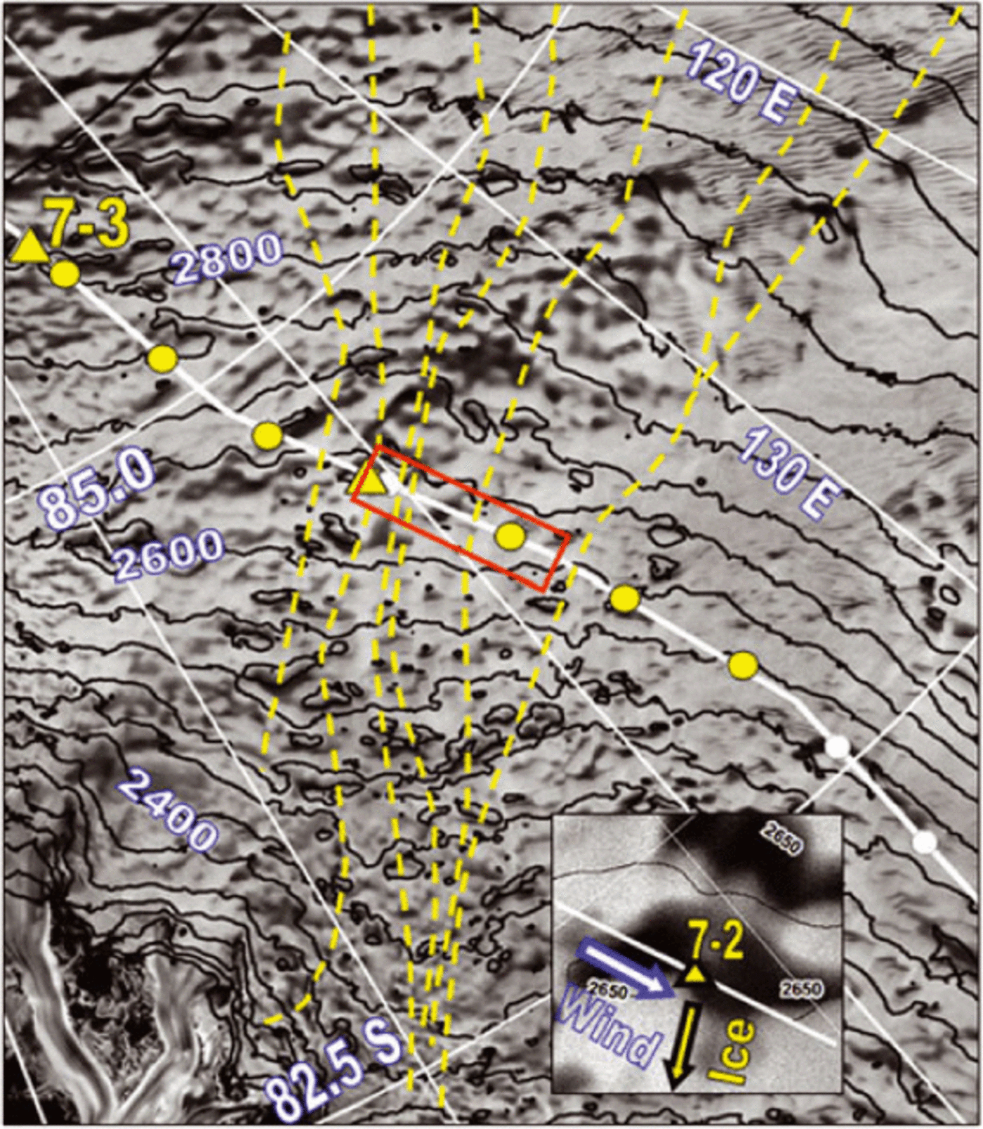
Fig. 6. Segment T1 (red box) and dashed ice flowlines superimposed on the 1997 RADARSAT image. Elevation contours are in 50m increments, and yellow dots are 50 km apart. Dune fields appear _130 km to the west. Katabatic wind direction is nearly parallel to T1. The inset shows the accumulation environment of site 7-2; the white diagonal line is 30km long
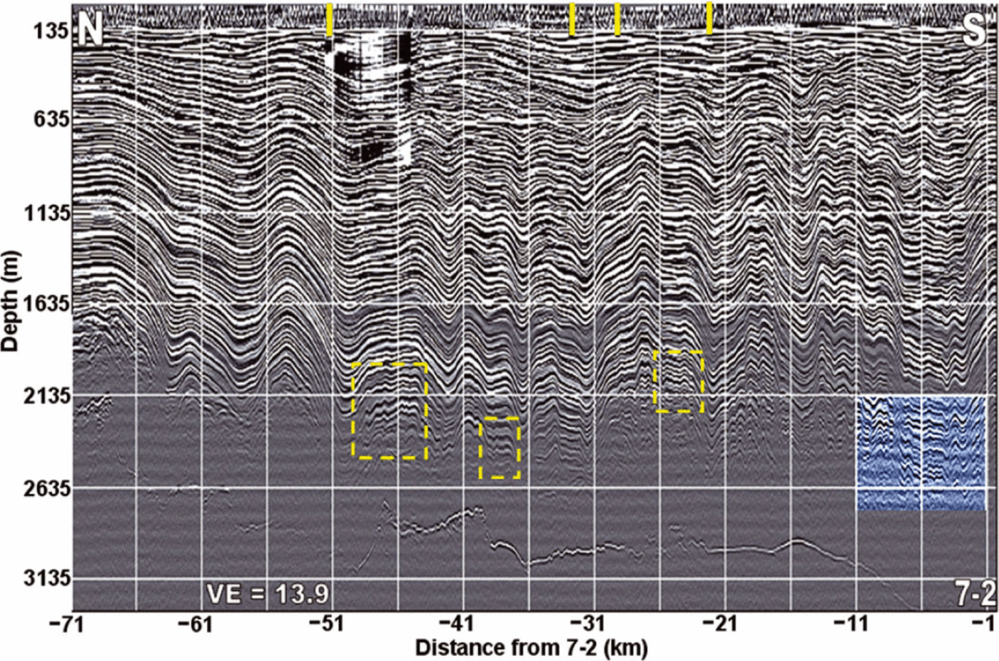
Fig. 7. 3.2 MHz englacial profile of the transverse folded section of T1. The depth scales are with respect to the top of the noise band. Flow is into the page. The yellow vertical lines locate flowline crossings in Figure 6. The dashed boxes enclose fine-scale folds superimposed on large-scale folds. The increased contrast in the box at lower right reveals the depth of the parallel folding.
The profile in Figure 7 is across ice flow. All horizons are unconformable because none lasts more than ˜30km before intersecting or apparently merging with another. In contrast with the profile of T4, all horizons are major because there are no visible bedding sequences. This suggests that the contained bedding sequences are thinner than the 40 m pulse resolution. This general lack of visible sequences is typical of our profile starting at 110km from site 7-1 and continuing for 540 km south.
The stratigraphy is strongly folded across the entire segment, which includes four of the flowlines of Figure 6. The folding begins at ˜200m depth. In some places fold limbs are nonparallel because they steepen with depth, such as from 0 to -3 km, -6 to -8 km, -22 to -23 km, and -50 to -53 km. However, much folding appears parallel for 2-3 km along the fold limbs and hinges. Most examples are from -9 to -21 km and -26 to -46 km below ˜1000 m depth. In the box section of Figure 7, to which we applied extra contrast, nearly parallel folding persists to >2600m depth. The dashed boxes enclose examples of sub-kilometer parallel folding superimposed on the larger folds.
4.3. T3 and T2: modified layers in the firn-englacial transition
The englacial profiles of Figures 4 and 5 show major horizons delineating cosets. From Part I it is clear that these horizons are associated with the modified recrystallized layers that first formed in firn. However, it is not clear if the modification affected acidic strata. We address this question next with the comparative profiles in Figures 8 and 9.

Fig. 8. (a) Segment T3 (red box) superimposed on a RADARSAT image, (b) 200MHz profile, (c) 10–20MHz profile of the firn– englacial transition, and (d) bottom topographic profile. The ice direction arrow in (a) is 10 km long. The arrow in (c) indicates the horizon we interpret as defining the bottom of this large, transversely synformal coset. The portion of the dotted box in (b) contains modified strata within which acidic-based horizons are revealed in (c).
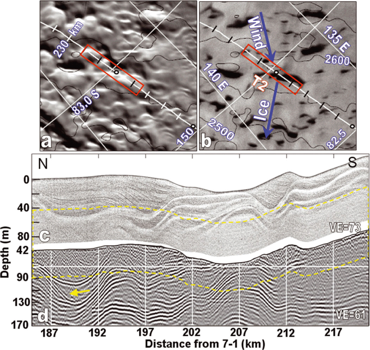
Fig. 9. (a) MODIS and (b) RADARSAT images of the environment of segment T2 (red box), and (c) 200MHz firn profile and (d) 10–20MHz profile of the firn–englacial transition. Distances along the traverse in (a) and (b) are measured from site 7-1, and elevation contours are in 50m increments. Irregular megadune-type features west of T2 are best seen in (a), while isolated accumulation features are best seen in (b).The strikes of the dunes are nearly normal to the modeled wind. In (c) and (d) ice flow is mainly into the page. The dashed box encloses the same depths within which there is loss of density strata in (c) but acidic strata remain in (d). The arrow in (d) indicates a bedding sequence confined by upper and lower modified layers.
Figure 8a depicts segment T3, which is 30 km long, orthogonal to ice flow and ˜35° to the modeled wind direction. From 105 to 110km T3 crosses the large accumulation feature seen in the RADARSAT image and situated over a large ice-bed depression with at least 450m of relief (Fig. 8d). T3 also crosses merging flowlines 80-120 km from site 7-1 (Fig. 3). Consistently, the 200 and 10-20 MHz profiles (Fig. 8b and c) show a large asymmetric synform with a fold axis that dips from about 2.4 to 3.1° to the north. Figure 8c shows that the synformal strata are underlain by an unconformable horizon (arrow), which we interpret as the lower delineating layer of this bedding sequence. Consequently this is a coset in transverse sectional view, with windward slope up-ice and likely situated over a large ice-bed depression.
Figure 8b shows that at 200MHz the southerly dipping firn-density beds on the northern flank cover ˜15km and reach at least 90 m depth. At 10-20 MHz in Figure 8c these beds appear as acidic-based horizons that end at the unconformable, stronger reflecting acidic-based horizon that continues to the southern flank where it rises and becomes conformable with the density-based horizons. By 114 km the 200MHz dipping beds on the southern flank contain several modified and recrystallized layers that become nearly horizontal below 42 m depth. By 60 m depth, there is no evidence of density stratification. In contrast, the 10-20MHz horizons that occur within the same depth section are generally parallel to the 200MHz unstratified layers, and so reveal that acid-based strata remain within modified and recrystallized firn.
Segment T2 is 185-220 km south of site 7-1 (Fig. 9a and b). The modeled wind direction is ˜40° off the traverse direction. Based on topographic contours, ice flow is 60° east of north, but could be as much as 77° based on an interpolation between the measured values at sites 7-1 and 7-2. In either case, ice flow is strongly oblique to T2. Megadune-type features within MODIS and RADARSAT images (Fig. 9a and b) appear ˜10km to the west, where their strikes are generally orthogonal to the modeled wind direction. Consequently, the radar profiles of Figure 9c and d are mainly transverse sections of cosets, so most horizons would be expected to appear generally horizontal.
The 200 MHz firn profile in Figure 9c is dominated by the recrystallized layers, which have grown and thereby merged to appear continuous across the entire profile, and large unstratified recrystallized zones from 42 to 90 m depth (the implications of the continuity are discussed in the appendix to Part I). In contrast, within the corresponding depth range, the 10-20MHz profile of Figure 9d shows many acidic horizons that generally track with the recrystallized layers in Figure 9c, especially between 192 and 211km. Similar tracking holds for all 10-20MHz horizons south of site 7-1. Although acidic horizons are weak within depth sections from 185 to 193 km and from 211 to 220km, they still conform to nearby upper or lower horizons. The cross bedding in the 10-20MHz profile near 187km (arrow) is evidence that the upper and lower horizons confine a bedding sequence.
5. Discussion
5.1. Modified layers
In firn, our comparisons between the two radar profiles within both Figures 8 and 9 show that acidic stratification is retained where recrystallization has removed density stratification. Consequently, after recrystallization, which is promoted by vapor transport after burial, an acidic signature of the original isochronal unconformity is retained. It is likely that some acidic modification has occurred because post-depositional decreases in concentration of chemical species in very near-surface firn have been attributed to reemission into the atmosphere and to diffusion (Reference PropositoProposito and others, 2002). In deep firn, recrystallization that accompanies compression obviously does not suppress conductivity in general, as evidenced by any englacial ice- sheet radar profile.
Englacially, the retention of acidic stratification is consistent with our interpretation of modified firn layers being the cause of major horizons. In Figure 4 many of the unconformable horizons have the same black-white-black (-+-) half-cycle polarity sequence as the bottom horizon, by which we mean the same waveform polarity sequence seen in Figure 2. Examples of this horizon waveform are in the D* inset of Figure 4 and in the C* detail of Figure 5a. This polarity sequence indicates a reflection either from an interface between a relatively low-a layer and one of higher σ below, or, as must occur above and below the C* sequence, of an embedded thin (much less than the 40 m long pulse resolution) layer with higher σ than that of the ice matrix (Reference Arcone, Spikes, Hamilton and MayewskiArcone and others, 2004). Despite the lack of visible stratification within the D* feature of Figure 4, the waveform of the horizon above it suggests that an embedded high-σ layer is the case for this feature as well.
The major, delineating horizons of cosets B, C and D in Figures 4 and 5a appear nearly continuous either because the sigmoidal acidic beds that make up these horizons have sufficiently turned over to preclude the ability of the 3.2 MHz pulse to resolve their change in slope, or because they are too close to be resolved, or both. In Figure 5a, the beds appear unconformable with the upper delineating horizon from 40 to 43 km, but nearly conformable with it from 43 to 45 km where their slope is closer to that of the delineating horizon. The inset of feature B* in Figure 4 shows an example where the inflection associated with the change in curvature between adjoining beds is resolved. The obvious acidic nature of the upper delineating horizons for features D indicates that the sigmoidal continuations of these acidic beds have likely thinned sufficiently from strain to preclude their resolution.
5.2. Parallel folding, and origin of T4 cosets
Segments T1 and T4 are the only segments along the entire traverse with this degree of folding. Parallel folding indicates constant vertical strain because layers maintain their thicknesses throughout the fold. Consequently, slip occurs along bedding planes, and in Figures 4 and 7 it appears to reach to within a few hundred meters of the bottom. In nonparallel folding, the steepening and lengthening of fold limbs with depth indicates increasing vertical strain with age (Reference Ng and ConwayNg and Conway, 2004). Both are present here, so the overall pattern suggests a history of stick-slip behavior. The deep harmonic and parallel folding in Figure 4 led us to assume the possibility that this transverse compression may have occurred throughout the ice-sheet thickness (as in Fig. 7) when it happened up-ice-flow, and that up-ice basal slip in the axial along-flow direction has historically permitted any large windward-slope accumulation features to stabilize over large subglacial depressions (Reference Budd and CarterBudd and Carter, 1971;Part I). Basal slip below deeply frozen and slow-moving ice has been documented (Reference Echelmeyer and WangEchelmeyer and Wang, 1987;Reference Cuffey, Conway, Hallet, Gades and RaymondCuffey and others, 1999).
These flowlines, speeds, evidence of up-ice basal slip and evidence in Part I for topographic stability of large accumulation slopes lead us to identify the large cosets in Figure 4 with the similarly labeled features A-C in Figure 3. The northern offset of these features from the flowlines projects their associated strata to cross T4. Cosets generated within megadune fields likely have thicknesses less than the 40 m resolution of our pulse. Consequently, we interpret the speckle features, A, across the top of the entire profile in Figure 4, as having originated before and within the megadune fields labeled A in Figure 3. These features begin about 100-125 km from T4 and are up to 600 m deep within the first 32 km from site 7-1. We identify features B and C in Figure 3 as the sources for cosets B and C in Figure 4. Cosets B are at about 400-800 m depth. Cosets C are at about 800-1500 m depth and within the folded regime, which suggests that they originated in the convergence zone that ends by ˜-240km west of T4 at 120° E in Figure 3. The red stippling in Figure 3 indicates plateaus we identified in 5 m (elevation) ICESat (Ice, Cloud and land Elevation Satellite) contours, and that lie just up-flow and generally downwind of some of the dark accumulation zones.
Assuming uniform vertical strain, an 800 m depth over ice 2600m thick and an average accumulation rate of 0.05 mw.e. a-1 represents ˜19120 years. At a distance of 240km from T4, this time translates to an average ice balance speed of 12.55 m a-1. As seen in Figure 3, from 240 to 50km going east toward T4 the elevation decreases from about 2970 m to 2650 m, for a total drop of ˜320 m. Then, over the last 50 km the elevation drops ˜190 m. This greater than 2x increase of surface slope means the ice speed greatly increased over the last 50 km to T4. Assuming an average speed of 5 m a-1 from 240 to 50 km and an average of 41 m a-1 after 50 km to bring the speed along T4 up to 87 m a-1 at site 7-1 only 50 km to the south, the average for the 240 km distance is 12.50 m a-1. This speed distribution gives an average of 19.4m a-1 over the 125 km distance to megadune fields, and places the first appearance of the megadune fields cosets at 300 m depth.
The up-ice flow and wind directions and the strikes of RADARSAT features B and C in Figure 3 suggest that cosets B and C in Figures 4 and 5a must be depicted in transverse section, similar to the asymmetric synformal section of the coset in T3 (Fig. 8). Further evidence that they are in transverse view comes from their bed and sequence lengths. From north to south, GPR cosets B are 8-15 km long with bed lengths <2.5 km, and cosets C are <10 km long and with beds <2.5 km long. These bed lengths are much shorter than those we profiled for the thick firn cosets in Figure 2 of Part I or than those we deduced in Part I to be as long as the windward slopes. Consistently, from 100 to 350 km in Figure 3, accumulation features B are about 5-8 km wide from east to west and up to 20 km long from north to south, and features C are 8-12 km wide and up to 75 km long from north to south. Consequently, their bed lengths, if projected along ice flow, would likely compare well with the RADARSAT east-to-west feature dimensions and be much longer than they appear in Figure 4.
We use our modeling approach of Part I to estimate an accumulation rate for coset C*. This approach assumes that accumulation rate is sufficient to maintain a windward slope over a fixed ice-bed depression. At its minimal depth of 850 m, and at 1750 m above the bed, the Nye model (Reference NyeNye, 1957;see also Reference Dansgaard and JohnsenDansgaard and Johnsen, 1969) for constant vertical strain translates 150 m thickness to a precompression ice thickness of 223 m near the surface at 2600m above the bed. Given that the profile of Figure 5a is a synformal section transverse to the axial plane, we then form an axial plane model in Figure 5b, with a bed length of 10 km, as per the across-strike width of features C in Figure 3. For an ice speed v =5m a-1 and 10 km bed length (exponential factor D =0.1 in Part I), peak and average (along the slope) accumulation rates of 0.18 and 0.09 m w.e. a-1, respectively, achieve 223 m thickness. As we found in Part I, these rates are significantly above estimated regional averages, which led us to conclude that they would only partially compensate for the widespread glaze of these regions if estimated regional accumulation rates of 0.04-0.05 m a-1 are to be realized.
6. Conclusions
Within the limitations of our 40 m pulse resolution, deeply buried cosets of bedding sequences are not common along our entire 650km long profile. Where they occur they indiate large accumulation features farther up the flank of the ice sheet, similar to what we present in Part I for firn cosets. Acidic stratification within formerly modified firn layers produces the major unconformable horizons that delineate these cosets. Consequently, any post-burial recrystallized growth (Part I) may not affect the true isochronal unconformable surfaces of the original glazed accumulation hiatus, as defined by any acidic horizon. We were fortunate that our 3.2 MHz radar was able to resolve so many of these cosets and unconformable horizons. Future englacial GPR profiling would greatly benefit from a shorter pulse to better resolve coset bedding, the structure within the unconformable delineating horizons, and the parallel nature of the folds. A 20MHz transient system would provide 6 m of vertical resolution, and even 150 MHz systems (Reference GogineniGogineni and others, 2001) have profiled englacial layering and the ice bed under deep ice.
We interpret the parallel aspect of the folding to indicate possible basal slip or stick-slip behavior at the time of coset formation. Basal slip implies surface topographic stability over large subglacial depressions, intensified accumulation, and that our large and ancient englacial cosets were generated beneath present accumulation features farther west at higher elevation. Velocity, accumulation and radar measurements along ice flow and over features B and C of Figure 3 would help verify this interpretation, and the presence of transverse folding in that area.
Unconformable strata must exist throughout and proximal to the Byrd catchment dune fields because the orientation and 650 km length of our traverse provide a large sample of up-ice englacial and firn strata. Similar englacial strata obviously exist down-ice of the traverse. The >2000 m depth that we profiled shows that the uneven processes of intensified accumulation on windward slopes and wind-glaze on leeward slopes, both within megadune fields and in their peripheral areas, have existed in this region for tens of thousands of years.
Acknowledgements
This research was supported by US National Science Foundation (NSF) Office of Polar Programs (OPP) grants 188643 (Arcone), 188987 (Jacobel) and 188765 (Hamilton). We thank Brian Welch for acquiring the 3.2 MHz radar data, and students at St Olaf College for assistance in the processing; Daniel Breton for recording and processing GPS data; Brian Tracey, Seth Campbell, Kristin Schild and Monica Palmer for satellite image processing; Ted Scambos for comments and suggestions; two anonymous reviewers;and Paul Mayewski for his organization and leadership of the ITASE projects. Permission to publish was granted by Director, Cold Regions Research and Engineering Laboratory.


