


Introduction
The a.c. response of HF-doped ice single crystals has been analysed in terms of three dispersions, the space-charge dispersion, the usual Dehye dispersion as observed in “pure” ice, and the high-frequency dispersion which was observed at low temperatures and high frequencies (Camplin and Glen, 1973). In the analysis, use of the complex conductivity plot (Grant, 1958) and a numerical fitting technique (Camplin, unpublished) produced values for the low-frequency conductivity, the high-frequency conductivity, and relaxation time of each dispersion.
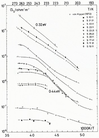
Fig. 1. (a) Temperature dependence of the Debye low-frequency conductivity, for pure and HF-doped monocrystals. The concentrations of the crystals are given in Table 1. Three samples from Von Hippel and others (1972) are shown for comparison; symbol V.
Fig. 1. (b) Temperature dependence of the high-frequency conductivity, for pure and HF-doped monocrystals. The concentrations of the crystals are given in Table I. Three samples from Von Hippel and others (1972) are shown for comparison; α∞ was calculated from measurements of σ0, τ and Δε.
The temperature dependence of the low-frequency and high-frequency conductivities for the dominant dispersion observed (identified with the usual Debye dispersion), σ 0 D and σ ∞ respectively, are presented in Figure 1. For reasons of clarity, only about half of the data set of 139 temperature and impurity combinations from 17 HF-doped ice single crystals are shown. The fluorine concentrations of all the samples investigated are shown in Table I. These are the concentrations obtained from the melted samples immediately after the electrical measurements were completed on each crystal. For experimental details see Camplin and Glen (1973).
Table I. Fluoride Concentration of each Crystal
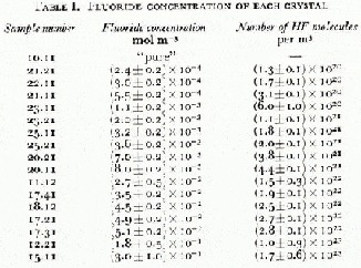
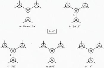
Fig. 2. Fluorine-centre configurations in ice doped with HF (b, c, d and e); the situation in pure ice (a) is given for comparison. The fourth bond of each molecule, which has not been shown, is normal and has its proton distant from the molecule. From Kröger (1974).
Defect Reactions
To understand our observations on HF-doped ice requires a full knowledge of the concentration of electrical defects that are introduced into ice by doping and their subsequent interactions. This paper will follow the terminology, notation and analysis of Kröger (1974) and assume that in ice the HF molecule may be found in any of four fluorine centre configurations (Fig. 2). The Bjerrum L defects and ionic ![]() defects generated from each centre and the dissociation equations which determine their concentrations are shown in Table II.
defects generated from each centre and the dissociation equations which determine their concentrations are shown in Table II.
Table II Defect Generation
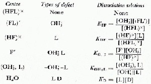
Kröger (1974) also considered the formation of complexes of ![]() and L defects forming a close association (
and L defects forming a close association (![]() , L). In addition to these equations, three further relationships exist to ensure charge neutrality and the D–L balance and to equate the HF content to the sum of the individual fluorine centres. Therefore, the concentrations of L, D,
, L). In addition to these equations, three further relationships exist to ensure charge neutrality and the D–L balance and to equate the HF content to the sum of the individual fluorine centres. Therefore, the concentrations of L, D, ![]() , OH′ and (
, OH′ and (![]() , L) defects may be derived for any temperature and HF concentration if the dissociation constants for the formation of the HF configurations and for the formation of Bjerrum and ionic defects are known.
, L) defects may be derived for any temperature and HF concentration if the dissociation constants for the formation of the HF configurations and for the formation of Bjerrum and ionic defects are known.
In addition, since the theory of electrical conduction in ice by Jaccard (1959) basically predicts a dielectric response of the single Debye dispersion form, then all the parameters of this dispersion, (ε s —ε ∞), σ 0, σ ∞, and τ may be determined once the concentration, mobility and charges of the Bjerrum and ionic defects are known.
Therefore, it is our objective to determine from our observations the concentration mobility, and charges of the Bjerrum and ionic defects using the theory of Jaccard, and then to estimate the dissociation constants for the possible reactions of HF in the ice lattice usine the analysis of Kroger.
Theoretical Models for Interpreting Observations
To develop in full a theoretical description of the behaviour of HF-doped ice based on the analyses of Kroger and Jaccard requires the knowledge of 24 parameters. We have simplified the analysis and taken advantage of two features which have been recognized before as being realistic of the behaviour of pure and doped ice.
We assume that the dissociation constant for ionic defects in pure ice is very low and in comparison with the defects introduced in laboratory “pure” or HF-doped ice, the intrinsic ions can be disregarded.
We also assume that the mobility of D defects is much less than that for L defects in the entire temperature range. Nevertheless, this condition is only important at high temperatures and low HF concentrations where L and D defects have comparable concentrations.
There is no doubt that σ 0 of the Jaccard theory should be identified with the low-frequency conductivity of the dominant dispersion, the Debye dispersion. However, there is an option of whether σ ∞ of the Jaccard theory should be identified with the high-frequency conductivity of the Debye dispersion or the high-frequency conductivity of the third dispersion when observed. We have decided to identify σ ∞ of the Jaccard theory with the limit of the highest frequency dispersion measured in our experiments on the assumption that the higher-frequency dispersion is related to some interaction between defects not allowed for in the Jaccard theory, and that, in the absence of such interactions, the dispersion strength would be the sum of the strengths observed.
In addition, we decided in the first instance to ignore the relaxation time predicted by the Jaccard model when comparing our data with theory because of the uncertainty in fitting his theory to our observations when two dispersions are present. However, as will be seen later, we found good agreement between the observed relaxation time of the dominant Debye dispersion and that calculated using the Jaccard theory.
These simplifications given above reduce the parameters needed in the Jaccard formulation from ten to six (see Table III). One parameter, the activation energy for the mobility of ![]() ions, we set equal to zero. The
ions, we set equal to zero. The ![]() mobility, μ
+, is weakly temperature dependent, increasing at low temperatures. A constant value for μ
+
? has been discussed by Camp and others (1969) and by Chen and others (1974).
mobility, μ
+, is weakly temperature dependent, increasing at low temperatures. A constant value for μ
+
? has been discussed by Camp and others (1969) and by Chen and others (1974).
Table III. Jaccard Theory Parameters

If T
m is the ice point, the mobility μ
L of L defects and μ
+ of ![]() ions at any temperature T are given by
ions at any temperature T are given by
and
We define the ionic conductivity σ ± and the Bjerrum conductivity σ DL by
and, from the Jaccard theory,
The calculation of [L], [![]() ], and [(
], and [(![]() , L)] from values of the simultaneous dissociation relations given in Table II is an extremely lengthy affair.
, L)] from values of the simultaneous dissociation relations given in Table II is an extremely lengthy affair.
We have simplified the calculations by deciding a priori that two or more of the fluorine configuration centres do not occur throughout the temperature range and therefore we fit the data with fewer variables.
Jaccard’s theory does not consider (OH3, L) associates. Such associates have been discussed at length by Onsager and Dupuis (1962), who argued that they are “sessile” and locked in the lattice. Therefore, they effectively remove mobile L and OH’ defects which could otherwise have contributed to the dielectric polarization and conductivity.
We concur with this view and take issue with Bilgram and Gränicher (1974) who believed that the associates have the properties originally attributed to the ![]() ion and can under certain circumstances be the dominant mechanism in dielectric relaxation, despite the fact that L defects are essentially involved in their movement.
ion and can under certain circumstances be the dominant mechanism in dielectric relaxation, despite the fact that L defects are essentially involved in their movement.
Therefore by comparing the best predictions of simpler models (see below) we would hope to decide the reactions through which Bjerrum L defects and ![]() ions are generated in HF-doped ice.
ions are generated in HF-doped ice.
Model 1
The simplest model to consider is the one for which only the fluorine centre configurations (HF)× and F′ exist. In this case, each HF molecule incorporated into the ice lattice generates a free L defect and the ![]() concentration satisfies the equation
concentration satisfies the equation
where F
TOT is the fluoride concentration. At high concentration this leads to ![]() .
.
Model 2
In this model we assume that the three fluorine centre configurations (HF)×, F′ and (HFL)× exist. This means there may be fewer extrinsic L defects than the total HF concentration depending on the value of the dissociation constant K
OF. The dissociation constant K
0, 1 determines the ![]() concentration, but the relationship between [
concentration, but the relationship between [![]() ], K
0, 1, and F
TOT only becomes more complicated than that in model (1) at the highest doping levels.
], K
0, 1, and F
TOT only becomes more complicated than that in model (1) at the highest doping levels.
Model 3
This model is one which is favoured by Bilgram and Gränicher (1974) and is a development of model (1). Only the fluorine centre configurations (HF)× and F′ exist, but the associated defects (![]() , L) are also found. This results (as in model (2)) in the extrinsic L defect concentration being less than F
TOT. Bilgram and Gränicher (1974) also proposed that the formation of Bjerrum defects in ice is given by
, L) are also found. This results (as in model (2)) in the extrinsic L defect concentration being less than F
TOT. Bilgram and Gränicher (1974) also proposed that the formation of Bjerrum defects in ice is given by
We believe there are strong reasons for not modifying [L] · [D] = K 0 and so the unmodified equation is incorporated into model (3a) and the modified equation into model (3b).
Results
We used a computer to vary the values of the unknown parameters in each model so as to minimize the deviation observed between experimental and model values of conductivity when conductivities are plotted logarithmically against 1/T. We therefore chose to minimize the RMS deviation, J, given by

for the N (normally 139) values each of σ 0 and σ ∞. Data taken from samples 23.21, 25.11 and 25.21 were inconsistent with data from neighbouring samples and appeared to have twice the HF content expected by interpolation. Thus, for the curve fitting, we assumed their concentrations to be half the recorded values.
The values obtained for the variables in the different models are shown in Table IV. All temperature-dependent variables are represented by the value at 0°C; the subscript m refers to this temperature. The quality of the fitting is given by the minimum value of J for each model, J min, and this has been converted to the RMS percentage error in the conductivity values, also tabulated in Table IV, by the expression too (exp J min—1). Models (2) and (3) fit better than the simplest model (1), yet the difference in the overall error is small, being 22% for model (1) and 20% for model (2). There are only small differences between the values derived for the nine parameters common to the three models, and essentially no difference between the common parameters of models (2) and (3).
Table IV. Best-Fit Parameters

It is worth considering the relative precision of the parameters that have been obtained in the analysis. Let X be the best-fitting value of one parameter x. When x = X, J = J min. In the neighbourhood of the residual minimum we have investigated the expected parabolic relationship of
where K is a constant of proportionality. From values of K for each parameter, we have determined the percentage changes (A) in the temperature-dependent parameters (actually calculated at the mean reciprocal temperature of our data (226 K)-1) and the activation energies and charges that would increase the value of J by 1% above the minimum J min. We have calculated these data for each model and find that the common parameters follow very similar statistics. The mean statistical values are displayed in Table IV. When examining the effect of altering the activation energy of a temperature-dependent process alone, the fitting constrained the process rate at 226 K to be unchanged. The activation energy changes (Δ) that are derived from values of A are also tabulated. The range in the values of activation energies found for the common parameters of all the models are of similar order to the Δ values derived for a 1 % change in J, corresponding to the percentage error in fitting σ 0 and σ ∞ increasing from 20.0% to 20.2%.
The dissociation constants K OF and K OH3L of models (2) and (3) do not play a crucial role in determining the overall fitting of the data with A values of 31% and 23%. Indeed, the absence of such interactions in model (1) does not lead to a poor fit of the data. The dissociation constant K 0, 1, with the A value of 1.3% is the most sensitive parameter in the analysis of all the models, whereas the dissociation constant K O, with the A value of 16%, determining the properties of pure ice, has far lower importance in this analysis of HF-doped ice.
The strength of the fitting programme is that we have considered the data as a whole. Previous interpretations of the behaviour of HF-doped ice have concentrated on specific features in isolation; for example, the linear relationship between σ ∞ and F TOT (Jaccard, 1959); the square-root dependence of F TOT on σ 0 at high fluoride concentrations (Jaccard, 1959), the linear relationship between σ 0 and F TOT at low concentrations (Camplin and Glen, 1973), and more recently, the temperature and HF-concentration dependence of the cross-over point (Bilgram and Gränicher, 1974).
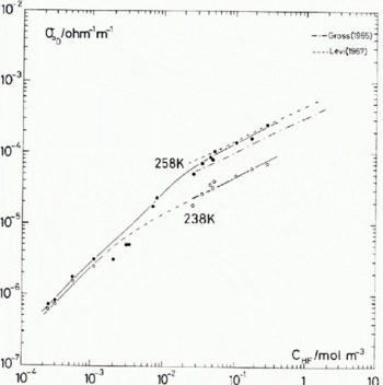
Fig. 3. Fluorine concentration dependence of the Debye low-frequency conductivity. The results from direct-current measurements made by Gross (1965) and Levi (1967) are shown for comparison.
To demonstrate the discrepancies that can occur when a specific feature is taken in isolation, consider the following results taken from Figure 3.
At 238 K,
At 258 K,
where N F is the number of HF molecules per cubic metre.
If the d.c. conductivity behaviour described by these equations is due solely to ionic defects, then we would have immediately the values of (μ
+/j
±) and K
0, 1 at these temperatures, where at low concentrations [![]() ] = F
TOT, at high concentrations [
] = F
TOT, at high concentrations [![]() ] = (K
0, 1
F
TOT)
] = (K
0, 1
F
TOT)![]() and σ
0D = e(μ
+/j
±)[
and σ
0D = e(μ
+/j
±)[![]() ]. In Table V we have compared the values obtained by this simple analysis with those obtained from the best fit of all the data using model (2).
]. In Table V we have compared the values obtained by this simple analysis with those obtained from the best fit of all the data using model (2).
Table V. COMPARISON OF ANALYSES FOR μ ±/j ± AND K0, 1

The difference between these two sets of (μ ±/j ±) and K 0, 1 is considerable and is due to the similar absolute values of σ + and σ L at 238 K and 258 K at fluoride concentrations above 1022 m-3. This is clearly shown in Figure 4 for the temperatures 198 K, 218 K, 238 K, 258 K, and 263 K using model (2).

Fig. 4. Values of the defect conductivities as a function of fluoride concentration at temperatures 198 K, 218 K, 238 K, 258 K, and 263 K, calculated using the best fit reaction parameters in the theoretical model 2* of Table IV.
The temperature dependence of the best-fit values of σ + and σ L using model (2) are given for four representative fluoride concentrations, 1.3 × 10²⁰ m-3, 1.0 × 10²¹ m-3, 1.9 × 10²² m-3, and 3 × 10²³ m-3 in Figure 5. In Figure 6 the predicted values of σ 0D and σ ∞ are compared with those observed in nine of the 17 samples used in the fitting. To include all samples in such figures would make the association of points and curves unclear. Those shown are a representative sample.
Discussion of Electrical Parameters
We now outline the major differences in the present values of the electrical parameters of HF-doped ice compared to those currently accepted.

Fig. 5. Values of the defect conductivities for four representative samples, 21.21, 25.21, 17.41, and 15.11, calculated using the best-fit reaction parameters in the theoretical model 2* of Table IV.

Fig. 6 (a) Experimental and calculated values of the Debye low-frequency conductivity for nine of the 17 samples investigated. The calculated values use the best-fit reaction parameters in the theoretical model 2* of Table IV.
Charges of Bjerrum and ionic defects
Our values of j DL and j ± have been obtained solely by analysis of the values of σ 0 and σ ∞ in HF-doped ice. Another estimate is available from the measurements of Camp and others (1969) which showed clearly for the first time in one nominally pure ice sample the cross-over in the majority defect mechanism as the temperature was lowered. From the data of σ 0 and σ ∞ supplied by Camp (personal communication) values of j DL = 0.423 and j ± = 0.796 are obtained. By comparison, an analysis of sample 23.11 of this study gave corresponding values of 0.402 and 0.773.
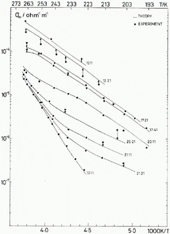
Fig. 6. (b) Experimental and calculated values of the high-frequency conductivity for nine of the 17 samples investigated. The calculated values use the best-fit reaction parameters in the theoretical model 2* of Table IV.
The value of j DL currently accepted is based on the measured value of the static permittivity of pure ice and that predicted by the Jaccard theory (Jaccard, 1959, 1964). Our calculation for j DL is wholly independent of such an argument.
From the best-fit values of j DL and j ± of 0.458 and 0.702, respectively, we derive through equations 1.7.4 and 1.7.12 of Jaccard (1959) the effective charges of the Bjerrum and ionic defects as 0.438e and 0.730e. Jaccard himself derived e DL/e = 0.43 (cf. equation 2.1.20; Jaccard, 1959) from measurements of the static permittivity in polycrystalline pure ice and by his theory required that e ±/e = 1 — e DL/e = 0.57.
No ice sample has been found for which at the cross-over temperature for majority defects there has been no dispersion in the audio-frequency range, yet the theory of Jaccard demands that there is no dispersion. Our higher value for e ± reflects the observation that in practice a small dispersion is observed, and our value of e DL entirely agrees with Jaccard’s value.
L-defect mobility
In figure 11 of Jaccard (1959), the linear dependence of σ ∞ and F TOT is displayed at —55°C (218 K). Assuming
we obtain from these data at 218 K,
From the computer analysis of our data (Table IV) we obtain
which at 218 K gives
The agreement with Jaccard’s value is excellent at this temperature of 218 K and, since the mean temperature of our data is 226 K, we have the greatest confidence in our predictions in this temperature range. Our samples were, however, more lightly doped and in our highest concentration range we did not observe a linear dependence of σ ∞, σ DL or σ + on doping; rather σ DL was proportional to the (F TOT) ≈ 0.75.
The activation energy for mobility in Equation (1) is 0.315 eV which may be alternatively written without the factor T m/T as
where E L ′ = E L—0.023 eV. This E L ′ value of 0.292 eV can be compared directly with that of 0.235 eV found in figure 12 of Jaccard (1959) and there is a major difference between the two values that is difficult to resolve.
Dissociation constant for Bjerrum defects, K 0
The activation energy for σ ∞ in “pure” ice, E σ∞ is given by
Our value of W 0 is 0.664 eV, so E σ∞ is 0.624 eV as found for our “pure” ice sample 10.11. Such a value exceeds the value of E σ∞ from Jaccard (1959) (0.575 eV) whereby Jaccard deduced 0.68 eV for W 0. Assuming D defects do not contribute to the Bjerrum conductivity, we calculate from Jaccard (1959) a value for K 0 of 5.44 × 1044 m-6 compared with 1.49 × 1044 m-6 at the melting point in our present analysis. The difference is small.
Ionic defect formation
At medium to high doping levels, all models lead to the ionic conductivity being proportional to ![]() and the activation energy for the ionic conductivity would be
and the activation energy for the ionic conductivity would be ![]() eV, which is 0.287 eV. This value is close to E
L
′ =0.292 eV, the activation energy for Bjerrum conductivity in the regime for which [L] = F
TOT. We can understand therefore the almost identical activation energies for σ
0 and σ
∞ in this doping range since both ionic and Bjerrum defect conductivities contribute to both measured conductivities.
eV, which is 0.287 eV. This value is close to E
L
′ =0.292 eV, the activation energy for Bjerrum conductivity in the regime for which [L] = F
TOT. We can understand therefore the almost identical activation energies for σ
0 and σ
∞ in this doping range since both ionic and Bjerrum defect conductivities contribute to both measured conductivities.
It has been found from Camplin (unpublished) that the function σ 0 σ ∞ behaves very simply with temperature over a wide HF concentration range (Glen, 1973).
If we consider the product σ DL σ ±, then at low concentrations when [H3O+] ≃ F TOT, σ DL σ ± is proportional to F TOT and the activation energy is
at medium concentrations when [(HF)×] ≃ F TOT, σ DL σ ± is proportional to (F TOT)≃ and the activation energy is
at the highest concentrations when [(HFL)×] ≃ F
TOT, σ
DL
σ
± is proportional to (F
TOT)![]() and the activation energy is
and the activation energy is
These values support the observations of similar activation energy for the product σ 0 σ ∞ throughout the doping range, yet the observed values for E σ0σ∞ are lower than those calculated for σ DL σ ± here.
Relaxation time, τ
With the values of σ DL, σ ±, e DL, and e ± obtained from the computer fitting, we may-calculate through equation 1.7.16 of Jaccard (1959) the relaxation time of the simple Debye dispersion anticipated by the Jaccard theory. In Figure 7 we compare these predictions with those of measurements from the dominant relaxation spectrum at the temperatures 218 K, 338 K, and 263 K. The agreement is good, and in part should be no surprise since our value of e DL correctly predicts the static permittivity of “pure” ice. However, the agreement does extend into the regime where there is no clear-cut predominance of one defect, and there the value of e ± plays an important role.

Fig. 7. Experimental relaxation times of HF-doped ice at 218 K, 238 K, and 263 K compared with the predictions of the Jaccard theory. The observations at the fixed temperatures were interpolated from measurements taken over a range of temperatures. Values found by Ruepp (1973) are also included for comparison.
Model (2) predicts from Figure 7 for the fluoride concentration range 3 × 10²² m-3 to 2 × 10²³ m-3,
and the activation energy E τ = (0.30±0.01) eV.
It is profitable at this stage to compare these results with data by Barnaal (1973) on the NMR relaxation time T 1 in samples containing in excess of 3 × 10²² m-3 HF; ? 1 ≃ F -(0.74±0.1) and E T1 = (0.25±0.015) eV.
We can show further that the NMR and dielectric behaviours are self-consistent within limits. The observed value of T 1 is proportional to the NMR correlation time, τ c. Once the constant of proportionality is known for the spectrometer used by Barnaal (1973), we may use his T 1 data to derive τ c in HF-doped ice. To do this, we compare Barnaal’s measurement of T 1 in pure ice of 1.05 s at 263 K with an independently calculated value of τ c, which for this analysis we take as (8 ± 2) × 10-6 s. The value of τ c at 263 K in pure ice has been calculated to be 11.5 × 10⁻⁶s by Siegle and Weithase (1969) and either 6.9 × 10⁻⁶ s or 9.0 × 10⁻⁶ s by Weithase and others (1971). It is expected to be identical with the jump time found in diffusion experiments using isotope tracers: 7.5 × 10⁻⁶ s (Ramseier, 1967).
We have used the T 1 data of figure 1 of Barnaal (1973) to produce the τ c data in Figure 8 where τ c is compared with the derived relaxation times at 243 K. According to Siegle and Weithase (1969), τ c = τ in ice for which electrical defects dominate the re-organization of neighbouring molecules. At corresponding HF concentrations in Figure 8 the ratio of τ c/τ is between 1.5 and 1.6; nevertheless systematic errors of around ±25% are expected in the value of τ c.
Despite the difference in the observed value of E τ and E T1, which give a temperature dependence to τ c/τ (see Table VI), it would seem reasonable to conclude that τ c and τ respond to the same internal motions. Measurements of T 1 and τ on the same samples would, of course, clarify whether there is any further systematic error in the estimate of fluorine content in different laboratories.
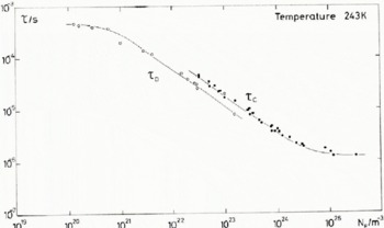
Fig. 8. NMR correlation time τ c and dielectric relaxation time τ d plotted as a function of HF concentration at 243 K.
Table VI. VALUES OF τ c/τ AT DIFFERENT TEMPERATURES

Conclusion
Despite the apparent good agreement between theory and experiment (Fig. 6), there is still considerable variation in behaviour observed between samples of adjacent fluoride concentration. This fact makes it difficult to differentiate between the predictions of models (2) and (3) to the extent we would have wished. This variation is especially crucial in the higher concentration samples where the predictions of the two models differ, and an incorrect assessment of fluoride content could lead to unrealistic values for the dissociation constants of the specific fluoride centres of each model. It would be most useful, therefore, to have further data at these higher doping levels. Such samples would provide data for further comparison with the NMR data of Barnaal (1973) shown in Figure 8, and the conductivity data of Jaccard (1959).
A disappointment with this analysis must be the surprisingly high value of 0.292 eV for E L ′, the activation energy for the mobility of L defects. This value exceeds Jaccard’s value of 0.235 eV, and our observations in Figure 1 (b) of 0.24 eV for σ ∞ in our most highly doped samples. In our fit of the σ 0 and σ ∞ data for all the samples, the highest discrepancy between models and observed data occur in this high-concentration range despite the extra freedom allowed in the fit by the choice of parameters describing the reactions of models (2) and (3). All attempts to reduce the value of E L ′ significantly led to a poorer fit of the data as a whole, although every other parameter was free to acquire correspondingly new values.
We feel that the defect conductivities derived from these models substantiate the theory of dielectric relaxation in ice proposed by Jaccard (1959). Inherent in Jaccard’s theory is the fact that the sum of the Bjerrum and ionic charges is the electronic charge, but the analyses of the data of Camp and others (1969) and that presented here do give a value around 1.2e. This discrepancy could be explained in a number of ways. If the samples analysed contain a defect-concentration gradient, then a dispersion would be observed, leading to e ± + e DL > e. On the other hand, the standard deviation between the experimental values of σ 0 and σ ∞ and those derived from our best models is 20%, and we feel that this aspect of Jaccard’s theory has not been disproved because of this uncertainty.
Discussion
M. ELDRUP: We believe we have shown that the vacancy concentration in ice is quite high. It may easily be higher than the concentrations of the defects you are discussing. Would interactions between vacancies and the defects which you discuss not change the results of your fit of your theory to the experiments? Would it introduce too many parameters to give useful results and thus confuse the situation rather than clarify it?
G. C. CAMPLIN: We have not considered the interaction between electrical point defects and vacancies, because we took the view that vacancies were less numerous. However, Kröger (1974) has given the necessary equations to accommodate such interactions and it is possible that our failure to fit the data to better than 20% in the three chosen models indicates that it is necessary to introduce further elements into the analysis. We will consider the implications of your results.
R. TAUBENBERGER: You claim that your defect models confirm to a certain extent Jaccard’s model but the requirement e DL + e ± = e is poorly fulfilled. Have you also plotted TΔε versus σ 0/σ ∞ which should give you a representation of dispersion data that are typical for this model (Jaccard, 1959; Hubmann, 1978)? If this plot fulfilled the features required by Jaccard’s model, you could work out e DL/e ± in a more self-consistent way, especially if you had sufficient ionic majority, i.e. sufficient low values of σ 0/σ ∞ (and high Δε values) after the first cross-over, and provided your Δε minima with their corresponding (σ 0/σ ∞) maxima represented at all cross-overs, the sense of Jaccard’s model.
CAMPLIN and J. G. PAREN: No. We have not plotted TΔε versus σ 0/σ ∞. However, we agree that if one considers the two intercepts on the ?Δε axis, then this plot leads to values of eDL/e ±. Nevertheless, absolute values of e DL and e ± can only be derived if an additional relationship (such as e DL + e ± = e) is also assumed. In our analysis, we have derived îDL and e ± independently of any additional relationship and our best-fit value of e DL/e ± is 0.600 compared to the value of Hubmann (unpublished) of 0.61 ± 2% derived from the diagrams of T·Δε against σ 0/σ ∞. The near identity of these two values of e DL/e ± shows that the methods of analysis used by Hubmann and by us are self-consistent. Of especial interest is that Hubmann’s charge-ratio value comes from an analysis of NH3-doped ice, and ours from HF-doped ice.
It is difficult to determine Δε at high concentrations and low temperatures because we have evidence for two dispersions instead of one predicted for the Jaccard model. Do we take the dispersion strength of both dispersions ?


