


1. INTRODUCTION
In line with global trends (Mernild and others, Reference Mernild, Lipscomb, Bahr, Radić and Zemp2013a), glaciers in South America have generally reduced in size since reaching their Little Ice Age maximums (~1850) (e.g. Georges Reference Georges2004; Casassa and others, Reference Casassa2007; Rivera and others, Reference Rivera, Benham, Casassa, Bamber and Dowdeswell2007; Masiokas and others, Reference Masiokas2008; Rabatel and others, Reference Rabatel, Castebrunet, Favier, Nicholson and Kinnard2011, Reference Rabatel2013; Malmros and others, Reference Malmros, Mernild, Wilson, Yde and Fensholt2016). Such behaviour results from the predominance of negative glacier mass-balance conditions (e.g. Gardner and others, Reference Gardner2012; Mernild and others, Reference Mernild, Lipscomb, Bahr, Radić and Zemp2013a) brought about by atmospheric warming and changes in precipitation patterns (e.g. Pellicciotti and others, Reference Pellicciotti, Burlando and Van Vliet2007; Falvey and Garreaud, Reference Falvey and Garreaud2009).
In addition to initiating lagged responses in glacier length and area, changes in mass balance also influence ice surface velocities as a glacier redistributes ice mass in an attempt to reach a new equilibrium. When mass balance is negative, ice velocities should reduce, as a result of reductions in ice deformation (mainly due to changes in ice thickness) and upstream stresses (due to there being less ice mass to transport), and vice versa when it is positive (Cuffey and Paterson, Reference Cuffey and Paterson2010). This relationship was demonstrated by Vincent and others (Reference Vincent, Soruco, Six and Le Meur2009), who recorded 20 a of thickening and velocity acceleration, followed by 30 a of thinning and velocity deceleration at Glacier d'Argentière, France. Long-term glacier velocity decreases observed in the Pamir and Caucacus mountains, Penny Ice Cap, Alaska Range, Patagonia and Southeast Greenland have also been attributed to negative mass-balance conditions (Heid and Kääb, Reference Heid and Kääb2012a; Mernild and others, Reference Mernild2013b).
However, the link between mass balance and ice velocity for some glaciers can be complicated by the influence of local topographic and climatic settings, subglacial hydrology and glacier surging behaviour, amongst other factors (Jobard and Dzokoski, Reference Jobarb and Dzokoski2006; Benn and others, Reference Benn, Warren and Mottram2007; Copland and others, Reference Copland2011; Sundal and others, Reference Sundal2011). For the Patagonian icefields, for example, climate-induced mass loss has been enhanced when outlet glaciers have switched into retreat phases of individual tidewater calving cycles (Rivera and others, Reference Rivera, Koppes, Bravo and Aravena2012). These retreat phases are initiated when tidewater or freshwater calving glacier fronts detach from local shallow pinning-points and recede rapidly into deep-water basins as a result of increased buoyancy and iceberg production (Post and others, Reference Post, O'Neel, Motyka and Streveler2011). Due to the subsequent reduction in resistive stresses at the glacier front, such phases are also accompanied by prolonged increases in glacier velocities (e.g. Upsala Glacier (49.70°S, 73.29°W); Mouginot and Rignot, Reference Mouginot and Rignot2015). There may also exist delays between mass balance and ice velocity fluctuations according to glacier size, bed slope and hypsometry (Oerlemans, Reference Oerlemans2008). Nevertheless, in the absence of detailed mass-balance records, ice velocity measurements acquired over long time periods can, in many cases, be a useful surrogate for assessing glacier health (long-term mass balance).
For South America, long-term glaciological mass-balance observations are spatially sparse, being limited to 22 glaciers and spanning the period 1976 to present (Mernild and others, Reference Mernild2015). To compensate for such under sampling, multi-temporal satellite data have been increasingly utilised to measure mass loss (e.g. Rignot and others, Reference Rignot, Rivera and Casassa2003; Gardner and others, Reference Gardner2012; Willis and others, Reference Willis, Melkonian, Pritchard and Ramage2012) and more prominently map glacier area and length fluctuations (e.g. Bown and others, Reference Bown, Rivera and Acuña2008; Davies and Glasser, Reference Davies and Glasser2012; López-Moreno and others, Reference López-Moreno2014; Paul and Mölg, Reference Paul and Mölg2014; White and Copland, Reference White and Copland2015). In comparison with the above analyses, long-term glacier velocity records are particularly sparse, being limited almost exclusively to the Patagonian Icefields. Using automated feature-tracking methodologies and repeat pass satellite imagery, a number of studies have now presented detailed glacier velocity and frontal position times series for the Patagonia Icefields revealing large inter-related annual fluctuations between 1984 and 2014 (e.g. Muto and Furuya, Reference Muto and Furuya2013; Sakakibara and Sugiyama, Reference Sakakibara and Sugiyama2014; Mouginot and Rignot, Reference Mouginot and Rignot2015).
North of the Patagonian Icefields (located between 46°40′ and 51°60′S), the long-term fluctuation in velocities for glaciers of the Andes Cordillera is relatively unknown, being limited to a small number of in-situ stake measurements made as part of on-going mass-balance programs (as reported in Gacitúa and others (Reference Gacitúa2015)). In regards to satellite-based observations, this lack of glacier surface velocity measurements in the southern, central and northern Andes can be attributed to (1) the comparatively smaller size of the glaciers and (2) the slow movement of many of the glaciers. The main outlet glaciers of the Northern and Southern Patagonia icefields, for example, have an average size of ~33 km2 (taken from the Randolph Glacier Inventory v.5.0 (RGI); http://www.glims.org/RGI/rgi50_dl.html) and can reach speeds >3 km a−1 (Mouginot and Rignot, Reference Mouginot and Rignot2015). In comparison, South American glaciers north of 46°40′S, have an average size >1 km2 (RGI v.5.0) and have been reported as flowing <3 m a−1 (e.g. Glaciar Olivares Alfa (33°11′S, 70°13′W); Gacitúa and others, Reference Gacitúa2015). Both the aforementioned points hinder the ability of automated feature tracking techniques to distinguish ice surface features from widely used medium resolution repeat pass satellite datasets (e.g. Landsat and Advanced Spaceborne Thermal Emission and Reflection Radiometer (ASTER) data: 15–30 m resolution).
Located in the central Chilean Andes, Glaciar Universidad (34.69°S, 70.33°W) is distinguishable from other glaciers in South America by (1) its relatively large size (estimated in this study to be 28.1 km2 as of 2015) and (2) the presence of band ogives on its surface (Fig. 1), which are discussed in Section 1.1. Utilising the movements of these band ogives, the aim of this study is to examine surface velocity fluctuations for Glaciar Universidad on an almost annual frequency between 1985 and 2015. This is achieved through the use of an automated feature tracking procedure applied to Landsat and ASTER satellite image pairs. The velocity observations were extended further through the manual analysis of declassified Corona reconnaissance imagery acquired in 1967 and 1969. Together, the Corona, Landsat and ASTER derived glacier velocities presented in this study represent the longest ice surface velocity time series currently available in South America, outside Patagonia. In addition to estimating ice surface velocity, the satellite data presented are used to map (1) frontal fluctuations and (2) temporal variations in the longitudinal width of surface ogive bands. The ogive analysis was performed in order to test the hypothesis that during periods of increased glacier velocities newly formed ogive bands should be wider. This hypothesis would support the ogive formation theory put forward by Nye (Reference Nye1958) (Section 1.1).
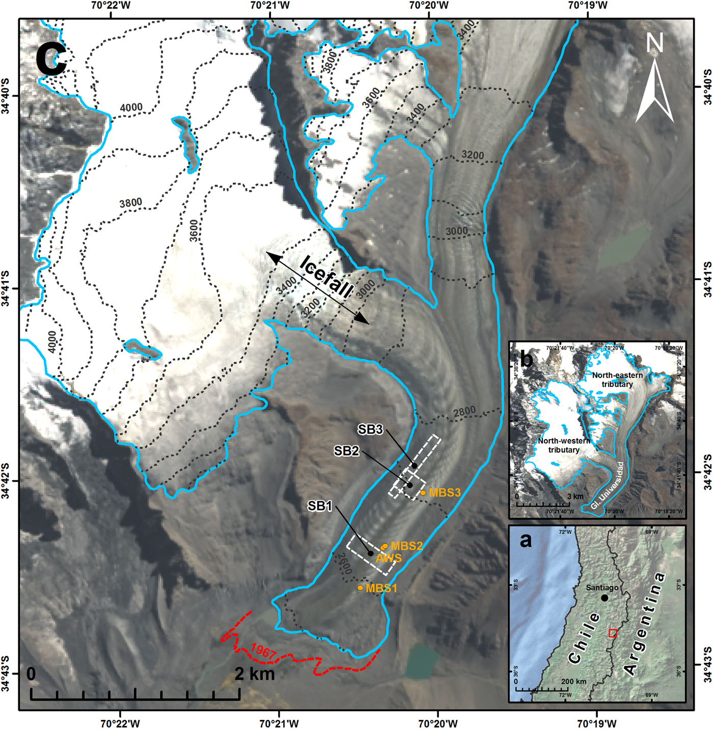
Fig. 1. Location and extent of Glaciar Universidad (highlighted in blue) in the central Chilean Andes (a, b, c). Ogive bands (consisting of alternate bands of dark and light ice) are shown flowing convexly down the main glacier trunk (c). These ogive bands are formed beneath the icefall, which intersects the North-western glacier tributary (c). The ice surface velocity (SB1 and SB2) and ogive width (SB3) sample boxes are marked by dashed boxes, while the location of the mass-balance stake (MBS, 1, 2 and 3) and AWS dGPS survey points (as of March 2009) are marked in orange (c). Background image: Landsat 8, 1 March 2015.
1.1. Formation of band ogives
Forming below steep icefalls on some glaciers, band ogives consist of alternating bands of dark and light ice. These alternating bands flow convexly down-glacier giving the surface of glacier ablation zones a striped appearance. The exact formation mechanisms of ogives are yet to be fully understood and currently several theories exist (discussed in detail by Leighton (Reference Leighton1951) and Goodsell and others (Reference Goodsell, Hambrey and Glasser2002)). One theory, proposed by Nye (Reference Nye1958), suggests that dark and light ogive bands are the result of the seasonal preferences in debris and snow acquisition of ice passing through icefalls. According to this theory, dark ice bands are formed during summer when heightened ablation of the stretched and fractured ice flowing down icefalls allows for the collection of more wind-blown debris. In contrast, light bands are formed during winter when excess snow collected in the large crevasses of icefalls is transported down-glacier. In this instance, a single ogive comprising a dark and light band is formed each glaciological year (central Chile: 1 April–31 March). According to this theory, ogive surface geometry would then be dependent on the ice surface velocity of the previous year.
An alternative ogive formation theory, proposed by Goodsell and others (Reference Goodsell, Hambrey and Glasser2002), suggests that ogives are the surface expression of shear planes. According to this theory, the rhythmic compression of flow at the base of icefalls results in zones of enhanced shearing along which basal ice and debris is uplifted to the surface via folding. These zones are subsequently characterised by areas of particularly dense foliation, which represent the dark ogive bands. This theory of ogive formation is supported by the ‘reverse faulting’ theory proposed by Posamentier (Reference Posamentier1978).
As indicators of glacier surface flow, band ogives are a useful feature for measuring ice velocities. The first detailed description of Glaciar Universidad and its ogive formations was published by Lliboutry (Reference Lliboutry1958). Through observing the movements of the ogive features, Lliboutry (Reference Lliboutry1958), for example, estimated that ice velocities for the central portion of the glacier were ~50 m a−1 in 1956, assuming that when flows are steady the distance between two band ogives gives the annual velocity.
2. DATA AND METHODS
Surface glacier velocity, frontal margin and ogive width analysis were performed with the use of two declassified Corona reconnaissance images, 33 Landsat 5 (Thematic Mapper) images, three Landsat 7 (Enhanced Thematic Mapper Plus) images, ten ASTER images and four Landsat 8 (Operational Land Imager) images acquired between 1967 and 2015 (Table 1). Where possible, images were chosen on the basis that they were cloud free, included minimum snow cover (typically at the end of the ablation season in February and March) and were acquired 1 a apart. Between 1999 and 2015, suitable imagery (medium resolution and cost effective) was available from the Landsat 5, Landsat 7, ASTER and Landsat 8 satellite archive. For the 2002 and 2003 observation periods, the Landsat 7 30 m sensor imagery was chosen over the 15 m panchromatic imagery available in order to (1) match with the resolution of the Landsat 5 imagery used and (2) limit CIAS (Correlation Image Analysis Software) bias introduced by comparing velocities obtained from image pairs of differing resolution. After 2003, the Landsat 7 image archive was not considered due to the failure of the sensors Scan Line Corrector (SLC). From 2013, the 15 m resolution Landsat 8 panchromatic imagery was preferred due to its improved geometric accuracy (Storey and others, Reference Storey, Choate and Lee2014). For the surface velocity analysis, imagery was also chosen based on the performance of the feature tracking procedure (Section 2.1).
Table 1. Satellite imagery used to derive ice velocities and map glacier front positions and ogive width variations
For the 2001/02 and 2002/03 observation period, the Landsat 7 15 m panchromatic imagery was used to map ogive widths and frontal margins.
IV, ice velocity; FM, frontal margin; OW, ogive width.
2.1. Surface velocity estimation
Glacier surface velocity fluctuations were estimated through the use of a feature tracking procedure based on automatic matching of image pairs. Several feature tracking or image matching techniques have been applied in earlier glaciological studies, including normalized cross correlation, Fourier cross correlation, least squares matching, phase correlation and orientation correlation (Kääb, Reference Kääb2005; Heid and Kääb, Reference Heid and Kääb2012b). Here, glacier velocity was estimated using the CIAS algorithm, which measures the displacement of surface features captured in overlapping satellite image pairs through Normalized Cross-Correlation (NCC) (Kääb and Volmer, Reference Kääb and Volmer2000; Heid and Kääb, Reference Heid and Kääb2012b). CIAS was chosen in this study due to its operational simplicity and good performance on glaciers with high-visual contrast (Heid and Kääb, Reference Heid and Kääb2012b).
NCC obtains a velocity measurement by systematically correlating a block of pixel values sampled from an initial reference image (first epoch) to pixel values contained within a larger search window area contained in an overlapping image (second epoch). Horizontal displacements and flow directions are then automatically calculated by comparing the centre location of the highest block correlation, found inside a search window, with that of the initial block. In this case, after testing the effect of window size variation on the frequency of displacement errors produced, it was found that a block and search window of 10 × 10 pixels and 25 × 25 pixels, respectively, performed consistently well for all image pairs used. Once generated, ice surface displacement errors were removed using (1) magnitude and flow direction filters, which eliminated velocity points that were abnormally high and did not adhere to the flow direction of the main glacier trunk, (2) CIAS-derived point correlation coefficients (deleting points <0.6) and (3) manual editing. To allow for cross comparisons, the remaining displacement points were scaled to annual velocities before being converted into 50 m × 50 m raster grids for analysis. When suitable image pairs were available from different sensors, velocity points were chosen for analysis based on the spatial distribution of successful points post error removal.
Due to their differing resolution, image quality and geometric distortions, CIAS was unable to estimate glacier velocity from Corona imagery. For the two Corona images used here a manual approach was applied, whereby distinguishable ice surface features were manually identified in each image and their displacement measured using standard GIS tools. Prior to measuring feature displacement, the Corona images needed to be orthorectified into a common WGS84 Universal Transversal Mercator (UTM) map projection. Following a similar method to that of Galiatsatos and others (Reference Galiatsatos, Donoghue and Philip2008), this procedure was performed using a non-metric camera model included within the Erdas Imagine Photogrammetry software module. Horizontal and vertical ground control points (GCPS) were manually obtained for the model from Landsat 8 15 m panchromatic imagery (acquired on the 10 January 2014) and the SRTM v.4.1 global DEM. The resulting horizontal RMSE for the Corona images equated to ±12 m.
In order to aid interpretation, the resulting glacier velocity points for each time period were extracted (1) along a longitudinal profile (positioned in relation to ogive visibility) and (2) in two sample boxes (SB1 and SB2) located between 2630–36 and 2700–20 m a.s.l., respectively (Fig. 1). Velocity points contained within the two sample boxes were then averaged for each time period. The two sample box locations were chosen where there was the greatest frequency of filtered velocity points in all 30 observations pairs.
2.2. Glacier frontal change and ogive width estimation
Fluctuations in the frontal position of Glaciar Universidad were calculated by manually measuring the difference in the location of terminus positions along a single polyline, following the central flow line, between each image in the 31 observation pairs (shown in Table 3). Additionally, the longitudinal width of individual ogive bands present along the central line of a third sample box (SB3; Fig. 1) were also manually measured for each separate image and then averaged (Table 2). The presence of debris cover within SB3 in the 1985 and 1986 images meant that ogive widths could not be measured. Overall, the number of individual ogive bands measured within SB3 ranged from 3 (1990–2000) to 7 (1967 and 2015) (Table 2). SB3 was located as close as possible to the icefall intersecting the main glacier trunk from its north-western tributary in order to measure the most recently formed ogive bands. However, this positioning was limited by the presence of snow cover close to the bottom of the icefall in the majority of the images acquired. For both the glacier front and ogive band measurements, the ASTER image pairs available for the 2005/06 and 2010/11 observations periods were preferred over the Landsat 5 alternatives due to their higher spatial resolution (Table 1). For the same reason, the 15 m Landsat 7 panchromatic imagery was used to measure these two variables in 2002 and 2003.
Table 2. The number and average width of individual ogive bands (consisting of a dark and light band) mapped longitudinally along the centre line of SB3
Table 3. Accuracy of the CIAS NCC-based feature tracking procedure assessed through the analysis of 1000 non-glacier displacements points calculated from each image pair observation date stated
Also included is the estimated horizontal errors attributed to the frontal change measurements presented.
* For the 1969–85 frontal change observation period, image co-registration (Corona to Landsat 5) was not performed. Therefore, a co-registration error of one Landsat 5 pixel was assumed.
2.3. Error and bias
2.3.1. Ice surface velocity error
For the Landsat 5, Landsat 7, Landsat 8 and ASTER derived glacier velocities, two main factors determined relative accuracy: (1) image co-registration accuracy; and (2) NCC image matching accuracy. In order to measure the first of these factors, each of the image pairs used were co-registered prior to image matching using a Helmert transformation, based on 50 GCPs sampled on stable terrain features located in close proximity to Glaciar Universidad. In this instance, error was taken from the RMSE of any horizontal image displacements. The accuracy of the NCC procedure was assessed through the RMSE calculation of 1000 non-glacier displacement points surrounding Glaciar Universidad in each of the image pair datasets. Error associated with each individual velocity image pair was then quantified through combining both the aforementioned RMSEs via error propagation. A summary of these errors for each of the satellite sensors used is given in Table 3. As NCC image matching was not performed for the Corona image pair, velocity accuracy in this case was based solely on image co-registration. Once orthorectified, the Corona image pair's co-registration RMSE was calculated using the horizontal displacements of 50 corresponding tie points (Table 3).
The availability of repeat differential GPS points (with horizontal accuracies of ~0.1 m), surveyed on three mass-balance stakes and one weather station located along the main glacier trunk (Fig. 1) between March 2009 and April 2010, allowed for an assessment of absolute error through comparison with the 2009/10 ASTER derived velocity dataset (Table 4). To perform this comparison, velocity measurements from the 2009/10 ASTER dataset were averaged within a 50 m radius of each of the 4 initial dGPS survey points. After scaling the measurements into annual velocities, the dGPS derived displacements were found to be consistently higher than the ASTER velocity measurements (+26%) with an RMSE equating to 16.2 m a−1 (Table 4). This absolute error matches similar comparisons made by other glaciological studies (e.g. Frezzotti and others, Reference Frezzotti, Capra and Vittuari1998; Redpath and others, Reference Redpath, Sirguey, Fitzsimons and Kääb2013) and, relative to the magnitude of the velocities shown for Glaciar Universidad, is considered to be small.
Table 4. Comparison of the 2009 with 2010 ASTER ice velocites, derived using the CIAS feature tracking algorithm, with mass-balance stake (MB1, 2, 3) and AWS repeat dGPS points surveyed over a similar period
One possible source of velocity bias that is not accounted for in this study is the effect of the differing temporal separations of the image pairs used. Although images were ideally acquired on an annual basis, captured at the end of the ablation season, these criteria were sometimes not met and the temporal separation of image pairs used ranged from 1021 (Corona) to 279 (ASTER) days. However, without knowledge of the interannual variations of ice velocities at Glaciar Universidad, the influence of temporal separation in this case was difficult to ascertain. Velocity bias may have also arisen from the cross comparison of velocities derived from satellite sensors with differing characteristics. Image matching techniques applied to Landsat and ASTER imagery, for example, have been found to be influenced, to varying degrees, by variations in sensor attitude (Heid and Kääb, Reference Heid and Kääb2012b) and horizontal shifts brought about by orthorectification errors (Heid and 2012a). Although these sources of bias are not accounted for specifically in this study, the cross comparability of the velocities presented is assessed through the comparison of displacement points derived from different sensors for approximately the same time period. Here, sensor cross comparisons were made for Landsat 8 and ASTER (2013/14), and Landsat 5 and ASTER (2005/06; 2006/07; and 2010/11) (Table 5). These four comparisons were chosen based on image pair availability, successful velocity point distribution and temporal separation. Overall, the RMSEs attained for each cross comparison (derived from overlapping velocity points) were found to be similar, ranging from 8 to 9.5 m a−1. Again, considering the magnitudes of the velocities shown for Glaciar Universidad, these cross sensor velocity differences are considered acceptable.
Table 5. Cross comparability of ice velocities derived from roughly same date Landsat 5, Landsat 8 and ASTER satellite image pairs using the CIAS feature tracking algorithm
2.3.2. Glacier frontal change and ogive widths
To calculate error in the frontal change measurements presented here, the method proposed by Williams and others (Reference Williams, Hall, Sigurdsson and Chien1997) and Hall and others (Reference Hall, Bayr, Schöner, Bindschadler and Chien2003) was utilised. Error in the linear direction (d) was therefore calculated using…
 $$d = \; \sqrt {r_1^2 + r_2^2} + {\rm RMSE}$$
where r 1 represents the spatial resolution (pixel cell width) of the first image of an observation pair, r 2 the spatial resolution of the second image and RMSE the image to image co-registration error. The resulting linear errors for frontal change measurements made from each observation pair are listed in Table 3. Error estimates presented for frontal change over a specified period (e.g. 1967–85) represent the average linear error of each observation pair included in that period.
For the ogive width measurements, a linear mapping error of one pixel was assumed for each ogive band measured within SB3. The total error attributed to the average ogive width measurements presented in Table 2 was then calculated via error propagation, depending on the number of ogive bands present within SB3 for a given year and the spatial resolution of the image used.
3. RESULTS
3.1. Surface velocity fluctuations between 1967 and 2015
Figure 2 presents the longitudinal satellite-derived ice surface velocity profiles for each separate observation interval between 1967 and 2015. Surface velocities for the main trunk of Glaciar Universidad are shown to be at their highest close to the bottom of the icefall, which connects the north-western tributary, before decreasing towards the ice terminus. In terms of annual surface velocity magnitude, Figures 2, 3 highlight four periods of transition for Glaciar Universidad. (1) Manual comparisons of ice surface features identified in Corona imagery acquired in 1967 and 1969 revealed average ice surface velocities of 91 and 134 m a−1 for the SB1 and SB2, respectively. These values for the 1967–69 period were similar in magnitude to the velocities estimated between 1993 and 1997. However, between 1986 and 1987 (2), representing a period of increased ice surface velocities, average velocities estimated for the higher elevation SB2 had increased by 91% in comparison with 1967–69 estimates, reaching 256 m a−1. After reaching a possible peak between 1986 and 1987, average annual ice velocities for SB1 and SB2 then underwent an abrupt deceleration up to 1993 (3), reducing by 64 and 58%, respectively. The following 22 a were characterised by a general trend of deceleration with velocities reaching a minimum during the 2014/15 interval. However, this period is marked by two relatively minor ice surface velocity acceleration events, the first occurring between 1993 and 1997 and the second occurring between 2001 and 2008. (4) Between 2008 and 2015, the rate of ice surface velocity deceleration then increases, with average values estimated within SB1 and SB2 reducing by 72 and 62%, respectively. Overall, the 2014/15 average ice velocities at SB1 and SB2 are shown to be 79 and 64% lower than estimated for the 1967–69 period, and 89% and 81% lower than the peak 1986/87 period, respectively. Considering Table 3, it is important to note that only long-term surface velocity changes beyond estimated errors (average of ±14 m a−1) are deemed significant.
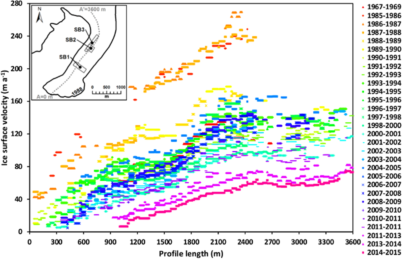
Fig. 2. Ice surface velocities extracted along a longitudinal profile (see inset: A-A′) of Glaciar Universidad between 1967 and 2015.
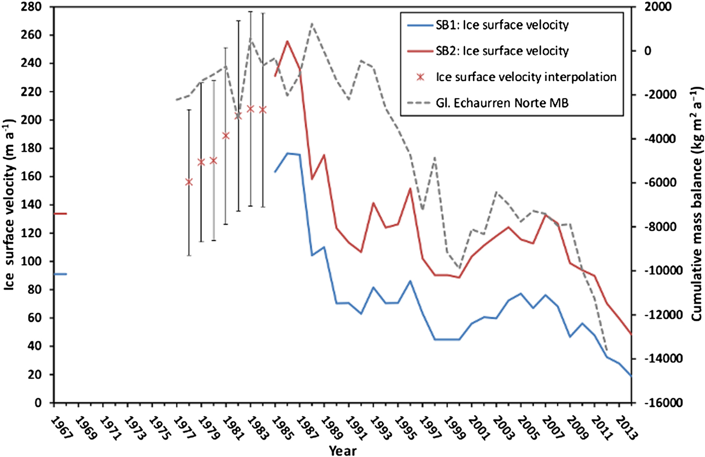
Fig. 3. Average ice surface velocity in SB1 and SB2 (location shown in Fig. 1) between 1967 and 2015. The ice surface velocity fluctuations measured for SB1 and SB2 show similarities with the mass-balance (MB) records available for Glaciar Echaurren Norte (1978–2012) located ~120 km north of Glaciar Universidad (sourced from the WGMS and Mernild and others, Reference Mernild2015). Y-axis point labels represents first year of observation pair (e.g. 1990 = 1990/91). Note that the 1999 point represents the 29 November 1998–28 January 2000 observation pair, while the 2011 point represents the 7 March 2011–11 December 2011 observation pair. Applying the linear relationship between the average ogive width time series, which had been adjusted back in time by 8 a (SB3: 1995–2015), and the ice surface velocity (SB2: 1985–2007) time series (Fig. 7), ogive widths measured between 1987 and 1993, prior to time adjustment, were used to interpolate ice velocities between 1978 and 1985, extending the ice surface velocity time series for SB2 by 7 a. Error bars indicate the level of uncertainty included within the coefficient of determination stated in Figure 7 (33%).
In addition to reducing near the glacier terminus, by 2014/15 annual ice velocities have also reduced considerably towards the north-western icefall, resulting in a lowering of the longitudinal velocity gradient for the main glacier trunk. The spatial distribution of annual velocity magnitudes for selected dates between 1985 and 2015 is shown in Figure 4, highlighting the extent of aforementioned velocity reductions. In addition, Figure 4 reveals that the ice dynamics of the main glacier trunk are largely governed by the north-western tributary. The influence of the north-western tributary (Fig. 1) is delimited by a longitudinal central moraine originating at the convergence point of the north-western and north-eastern tributary (Fig. 5). Annual surface velocities for ice flows west of this moraine limit are consistently higher for all observation intervals and coincide with the location of the ogive features present on the surface of the main glacier trunk.
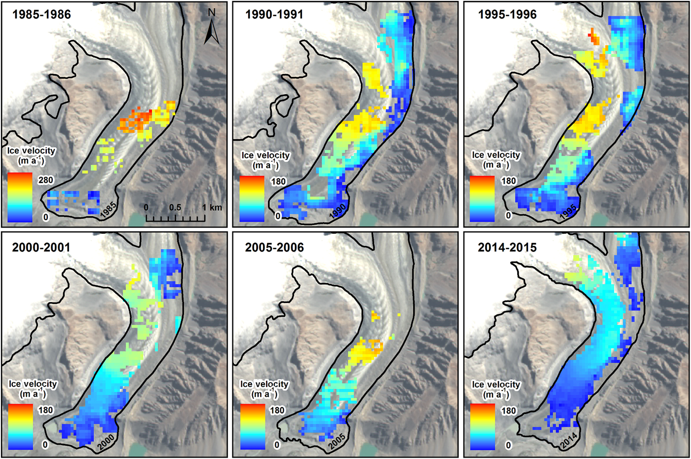
Fig. 4. Spatial distribution of selected ice surface velocity magnitudes. Note the larger ice surface velocity scale for the 1985/86 observation period.
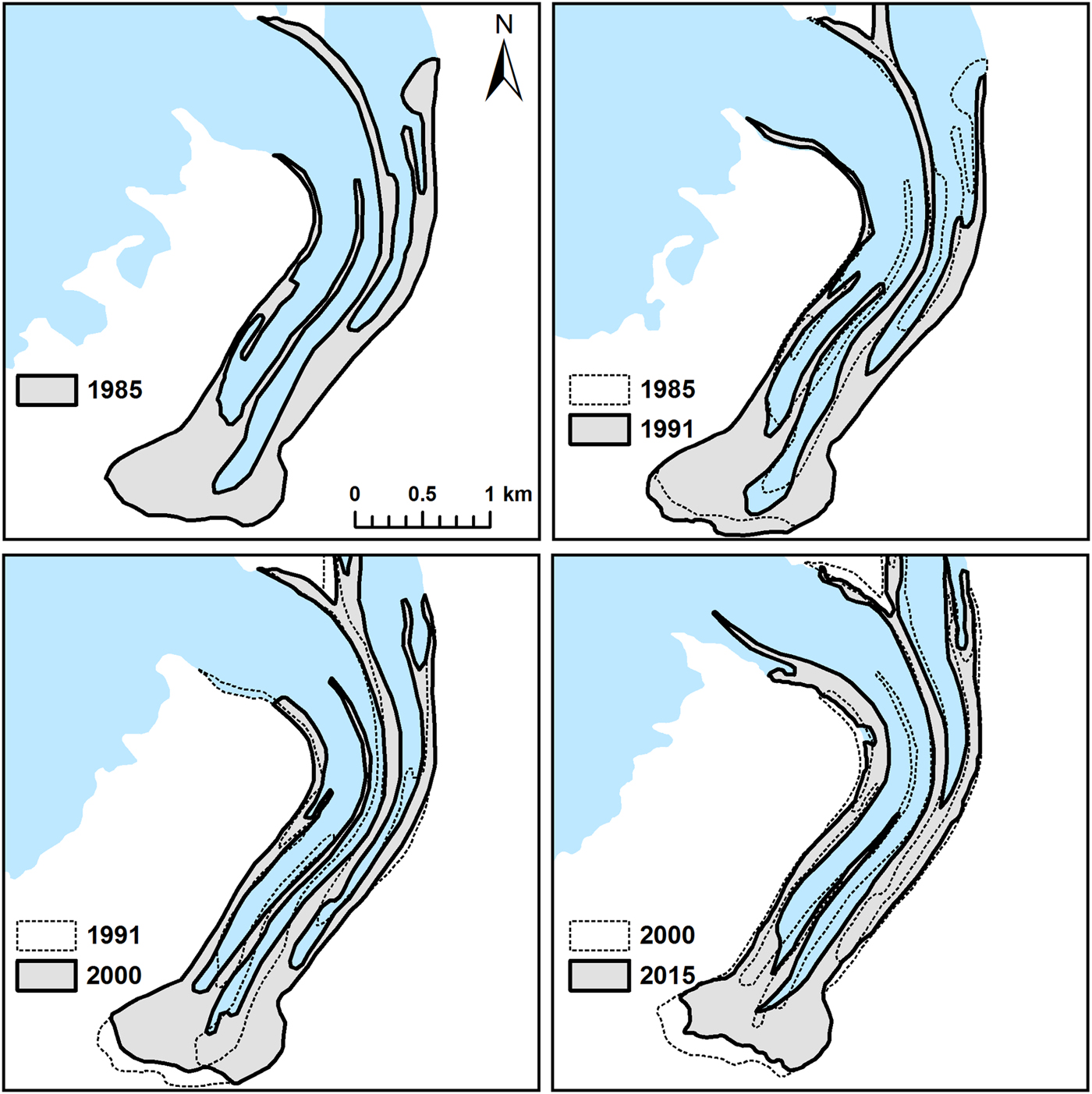
Fig. 5. Extent of ice surface moraines on the main trunk of Glacier Universidad in 1985, 1991, 2000 and 2015. Ogive bands have been omitted to improve the visibility of temporal movements in the moraines delineated.
By tracking the temporal movements of surface moraines on Glaciar Universidad further information can be sought in regard to the characteristics of the ice surface velocity changes measured during the observation period. Most notably, despite being slower than the surface flow attributed to the north-western tributary, surface flows attributed to the north-eastern tributary may have also been increased during the 1985–88 period, indicated by the development of a bulge in the central moraine running along the main glacier trunk (see 1991 moraine map in Fig. 5). From 1991 onwards, the influence of the north-eastern tributary on the ice dynamics of the main glacier trunk is shown to continually diminish, marked by the gradual eastern migration of the main central moraine. By 2014/15, for example, ice flows from the north-eastern tributary are generally reduced to <15 m a−1 at the convergence point with the north-western tributary.
3.2. Glacier front fluctuations and ogive widths between 1967 and 2015
A comparison of surface velocity and glacier front fluctuations for Glaciar Universidad revealed that the latter variable is fairly responsive to the former, with frontal fluctuations generally lagging behind surface velocity changes by 2 a. This frontal fluctuations lag is indicated by a peak cross correlation r 2 value of 0.65 (Fig. 6). For example, after retreating by 177 ± 36 m between 1967 and 1985, the glacier front advanced by 147 ± 18 m between 1985 and 1988 corresponding closely to the period of increased surface velocities observed during 1985/86 and 1986/87. Following this event, two other minor periods of advance occurred between 1996–98 and 2004–08, these events matching periods of surface velocity increase observed between 1994–97 and 2000–05. Despite these periods of advance, frontal retreat has predominated since 1988, with the glacier reducing in length by a cumulative total of 465 ± 44 m between 1967 and 2015.
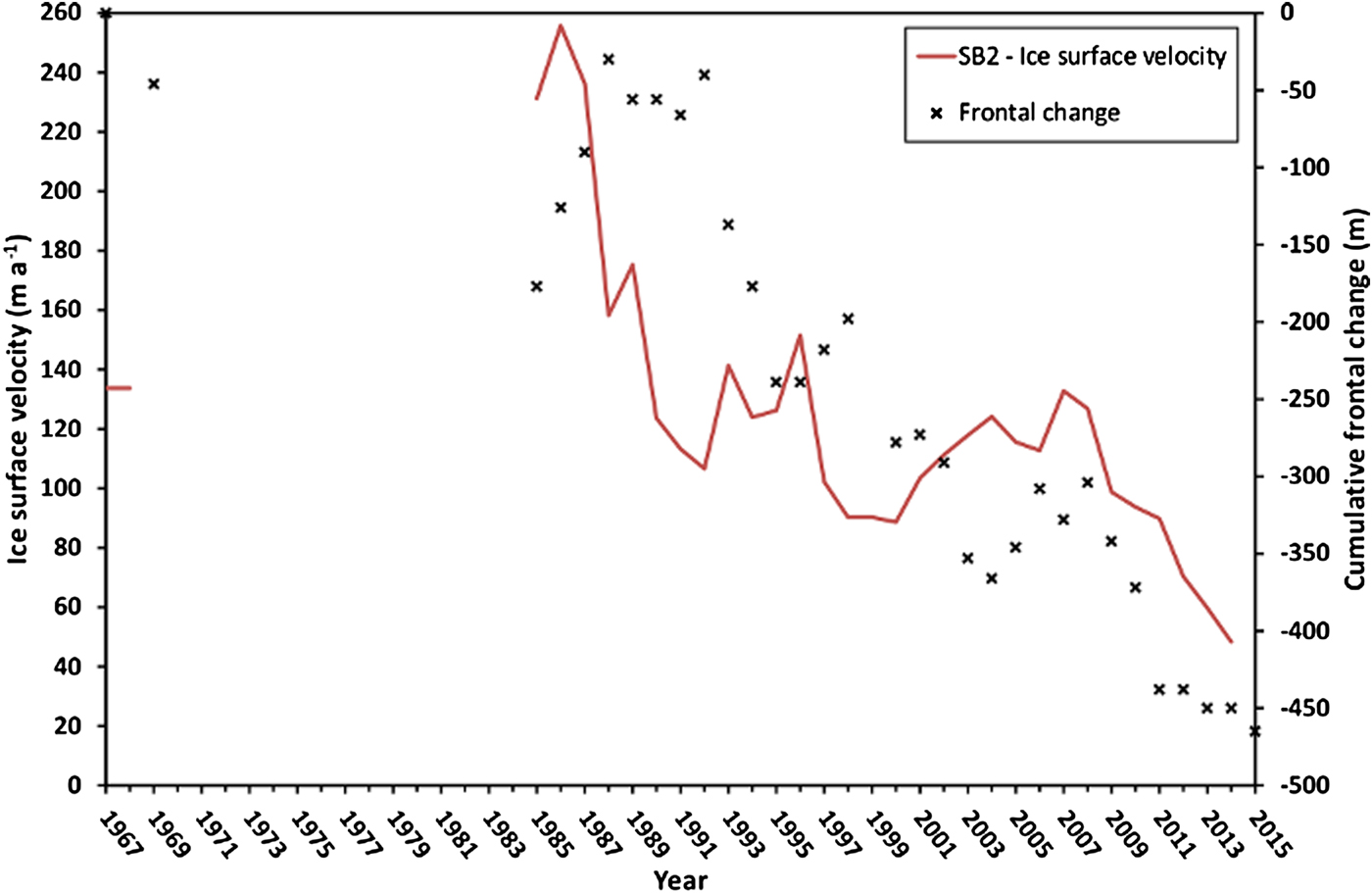
Fig. 6. Cumulative frontal change of Glaciar Universidad, between 1967 and 2015, compared with ice suface velocity fluctuations measured for SB2 (location shown in Fig. 1). Y-axis point labels for frontal change represent second year of observation period (e.g. 2015= frontal change between 2014 and 2015). Y-axis point labels for ice surface velocity are the same as stated in Figure 3.
Average ogive widths measured within SB3 are shown in Figure 7. Considering the ogive formation theory put forward by Nye (Reference Nye1958), it was expected that longitudinal ogive width would be larger when annual ice velocities were increased. Here, this relationship was complicated by the location of the ogive width SB3 ~1600–2300 m down-glacier of the formation zone at the icefall bottom. Consequently, ogive widths measured in SB3 for a given observation year likely indicate surface flow characteristics from previous years. Unfortunately, in this case the quantification of a precise ogive width lag time was hindered by the inability to track individual ogives close to the icefall, as this area was often covered in snow. In order to obtain a first order approximation of the relationship between ogive width and ice surface velocity, an 8 a lag was therefore assumed by matching the 1986/87 surface velocity peak to the ogive width peak observed for 1995. A subsequent Pearson's correlation between the adjusted ogive width time series and the corresponding ice surface velocity time series measured at SB2 (1985/86 to 2006/07) showed a significant r 2 value of 0.67 (explaining 67% of the variance) (p < 0.05; where p is the level of significance) (Fig. 7). To perform this correlation, firstly, surface velocities for both the 1997/98 and 1998/99 time periods were assumed to be 102 m a−1. This initial assumption was made with reference to the annual ice surface velocity estimated for the 3 January 1997–29 November 1998 observation period. Secondly, once adjusted, surface velocity and average ogive width data for the 1990/91 time period were withdrawn due to ogive width measurements not being available for the non-adjusted 1999 data point.
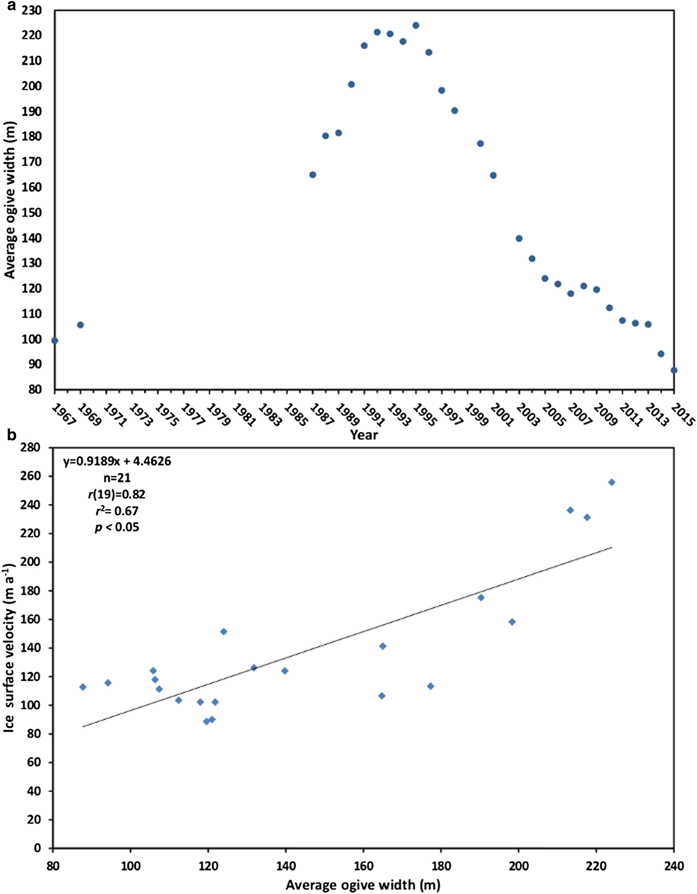
Fig. 7. Average ogive width measured within SB3 (location shown in Fig. 1) between 1967 and 2015 (a.) and the linear relationship between average ogive width (SB3: 1995–2015) and ice surface velocity (SB2: 1985–2007) (including statistical information, where n is the number of data points used, r is Pearson's correlation (with the degrees of freedom in parentheses), r 2 is the coefficient of determination and p is the level of significance (b). A time adjustment of −8 a was applied to the ogive width time series in order to offset the distance newly formed ogives have to travel to before reaching SB2 (Section 3.2).
Using the 8 a time adjustment there was then an opportunity to estimate ice velocities between 1978 and 1984 through the application of a simple linear regression model (see interpolation data presented in Fig. 3). The resulting ice surface velocity interpolations suggest that the 1986/87 period represents the peak of a period of ice surface velocity acceleration.
4. DISCUSSION
In light of the temporal and spatial limitations of current glacier mass-balance datasets in the Andes Cordillera, one of the main aims of this study was to construct a long-term surface velocity record for Glaciar Universidad that could provide useful information for assessing glacier health. For steady-state glaciers, for example, ice velocities are strongly linked to mass balance, with the mass flux through a cross section of a glacier equalling the upstream mass balance (Paterson, Reference Paterson1994; Heid, Reference Heid2011). For Glaciar Universidad, however, this link is complicated by the observation of possible surge behaviour in 1943 (Lliboutry, Reference Lliboutry1958). Triggered by internal glacier instabilities related to basal hydrology and thermal conditions, amongst others factors (Meier and Post, Reference Meier and Post1969; Björnsson, Reference Björnsson1998; Dunse and others, Reference Dunse2015; Sevestre and others, Reference Sevestre, Benn, Hulton and Bælum2015), glacier surging events are often de-coupled from local climatic forcing (Raymond, Reference Raymond1987). In one scenario, the surface velocity fluctuations presented between 1967 and 2015 may thus only indicate different stages of a surge cycle (e.g. Melvold and Hagen, Reference Melvold and Hagen1998) and would be of limited use for assessing changes in mass-balance conditions.
The abovementioned scenario, however, is challenged by the synchronicity of the surface velocity and glacier front fluctuations shown in this study with (1) the mass-balance records of the nearby Glaciar Echaurren Norte, which is located ~120 km North of Glaciar Universidad (33.57°S, 70.13°W) and (2) other glacier and climate observations available in the central Andes Cordillera. Available since 1976, Glaciar Echaurren Norte has the longest direct mass-balance record available for the Andes Cordillera (data presented in Fig. 3 are sourced from the World Glacier Monitoring Service (WGMS) (http://www.wgms.ch) and Mernild and others, Reference Mernild2015). Analysis of these records reveals periods of sustained positive mass balances in the 1980s and to a lesser extent in the 2000s (WGMS, Reference Zemp2013; Masiokas and others, Reference Masiokas2015). Mass-balance data for 1983, for example, was >10 orders of magnitude greater than the overall mass-balance mean observed for Glaciar Echaurren Norte. In comparison with the 1980s and 2000s, mass-balance observations in the 1990s were largely negative, the overall pattern matching closely the surface velocity and glacier front fluctuations shown for Glaciar Universidad (see Figs 3, 6).
Advance behaviour similar to that shown for Glaciar Universidad has also been observed for a number of glaciers located in the central Andes Cordillera. Glaciers of the Rio Plomo basin Argentina (~33.12°S, 69.98°W), for example, underwent a general reactivation between 1982 and 1991, characterised by rapid frontal advances (Llorens and Leiva, Reference Llorens and Leiva1995; Llorens, Reference Llorens, Trombotto and Villalba2002). Likewise, the glaciers surrounding Cerro Tupungato (33.35°S, 69.77°W) were shown to have advanced between 1982 and 1985 (Llorens and Leiva, Reference Llorens, Leiva, Smolka and Volkheimer2000). Glaciar Horcones Inferior (32.68°S, 69.97°W) also experienced advances of several kilometres during the 1980s, and again between 2004 and 2006 (Unger and others, Reference Unger, Espizua and Bottero2000; Llorens, Reference Llorens, Trombotto and Villalba2002; Espizua and others, Reference Espizua, Pitte and Ferri Hidalgo2008).
Although glaciers in the central Andes Cordillera have been generally reducing in area over the past few decades, the corresponding periods of advance for Glaciar Universidad and other glaciers in the central Andes region, particularly during the 1980s, suggests the direct influence of favourable climatic conditions. Snowfall analyses, for example, indicate a higher frequency of above average winter snowfall accumulation in the central Andes Cordillera since 1976 (Masiokas and others, Reference Masiokas2009), with particularly large snow accumulation events occurring between 1980 and 1985 (Masiokas and others, Reference Masiokas, Villalba, Luckman, Le Quesne and Carlos Aravena2006). These observations agree with the positive trend in rainfall measured for central Chile between 1970 and 2000 (Quintana, Reference Quintana2004), and 1979–2014 (Mernild and others, Reference Mernild2016). However, the influence of increased precipitation on glacier mass-balance conditions in the central Andes Cordillera has likely been offset through time by rising air temperatures reducing the amount of precipitation falling as snow. Falvey and Garreaud (Reference Falvey and Garreaud2009) and Mernild and others (Reference Mernild2016), for example, observed warming rates of 0.25°C (10 a)−1 between 1976 and 2006. Furthermore, in the 1990s, air temperature increase for the central Andes Cordillera coincided with a number of extreme drought events in central Chile (Quintana, Reference Quintana2000), which may have brought about negative mass-balance conditions, accounting for the reduced ice velocities observed for Glaciar Universidad during this period. If indeed the ice surface velocity and glacier front fluctuations shown are a direct response to climatic changes, the results presented here suggest that Glaciar Universidad has experienced increasingly negative mass-balance conditions since 1986, which were only partially reversed during the 1993–97 and 2001–09 periods before reducing further between 2009 and 2015. Such mass-balance behaviour agrees with what is shown for Glaciar Echaurren Norte.
The longitudinal width of the ogives present on the main trunk of Glaciar Universidad was temporally measured under the assumption that larger widths indicate higher ice surface velocities. After applying a time adjustment in order to offset the distance newly formed ogives have to travel to reach the sample box used, the surface velocity and ogive width measurements presented were shown to generally agree with the abovementioned assumption. Using this relationship, average ogive widths measured within a sample box between 1987 and 1993 could be used to interpolate ice velocities between 1978 and 1984, extending the velocity time series presented by 7 a. These interpolations suggest that the 1986/87 period represents the peak of a period of relatively increased ice surface velocities that began in the mid to late 1970s. However, these ice surface velocity interpolations contain a large amount of uncertainty and only represent a first-order approximation. In particular, the interpolations presented do not take into account the influence of temporal changes in compressional strain rates on the ogive width dataset presented. Such changes have likely occurred due to (1) changes in surface slope as a result of ice thickening and thinning, (2) changes in the longitudinal velocity gradient of the main glacier trunk and its north-western tributary and (3) changes in the ice flow influence of the north-eastern tributary. Additionally, the interpolations presented include ogive width mapping errors introduced through the use of relatively coarse satellite imagery. However, despite the aforementioned limitations, this study demonstrates the potential of surface ogive monitoring as a tool for assessing past glacier surface flow characteristics and should encourage further investigation of the relationship between these two variables using high-resolution satellite imagery and/or field based surveys.
5. CONCLUSION
Analysis of the remotely sensed datasets used in this study provides the following conclusions:
-
(1) The main trunk of Glaciar Universidad experienced a large increase in ice surface velocity between 1967 and 1987. Rather than being confined to the north-western tributary, which dominates the ice flow of the main glacier trunk, moraine mapping suggests that the north-eastern tributary also underwent increased ice flows between 1967 and 1987. Following 1987, the main glacier trunk experienced a considerable surface velocity deceleration, with the 2014/15 period representing a possible 48 a low. This period of deceleration was interrupted by two periods of minor velocity increases from 1993 to 1997, and 2002–08.
-
(2) Monitoring of the glacier terminus between 1967 and 2015 reveals that frontal fluctuations are fairly responsive to changes in ice surface velocity, responding with a 2 a lag between 1985 and 2015. In total, Glaciar Universidad experienced a 465 ± 44 m cumulative frontal retreat between 1967 and 2015.
-
(3) Assuming that the longitudinal width of ogives increases in response to accelerated ice surface velocities, ogive measurements obtained between 1987 and 1993 were used to interpolate ice surface velocity conditions between 1978 and 1984, extending the ice surface velocity time series presented by 7 a. Although only a first order approximation, this analysis suggests this assumed relationship to be true and highlights the potential use of glacier ogives to predict past ice flow characteristics.
-
(4) Although having exhibited possible surge behaviour around 1943 (Lliboutry, Reference Lliboutry1958), the synchrony of the glacier changes presented for Glacier Universidad with those reported for nearby glaciers suggests that this glacier is responding directly to climatic trends. If the above assumption is true, the results presented indicate a general pattern of increasingly negative glacier mass-balance conditions since the late 1980s. This pattern would match that shown in the mass-balance records (1978–2012) available for the nearby Glaciar Echaurren Norte (central Chilean Andes).
-
(5) The automatically derived ice velocities presented were shown to compare well with repeat dGPS survey point movements (±16 m a−1), further validating the use of the CIAS feature tracking algorithm for estimating ice flow from satellite imagery. Despite the variation in image and sensor characteristics, error analyses also revealed close similarities between ice velocities derived from Landsat 5, Landsat 8 and ASTER satellite image pairs for roughly the same date, highlighting the cross comparability of CIAS displacements measurements taken from different sensor platforms.
ACKNOWLEDGEMENTS
We thank the anonymous reviewers for their valuable critique of this article. The authors gratefully acknowledge the U.S. Geological Survey (Landsat imagery) and NASA Land Processes Distributed Active Archive centre (ASTER imagery) for free data access. We also thank Centro de Estudios Científicos (CECs) for the surveying of dGPS points during field campaigns conducted in 2009 and 2010. This work was primarily supported by CECs, which is funded by the Chilean Government through the Centers of Excellence Base Financing Program of Comisión Nacional de Investigación y Tecnológica de Chile (CONICYT). Additional funding for this publication was also made available from: (1) the National Science Foundation of Chile (FONDECYT) under Grant Agreement #1140172; and (2) the Research Councils UK (RCUK), Natural Environment Research Council (NERC) and CONICYT under project code NE/N020693/1. RW outlined the study, analysed the data and wrote the manuscript, with revisions from SHM, and JKM provided the frontal fluctuations data. CB and DC assisted with data collection and analysis. We would also like to thank Monica Pinto (University of Chile) whose work on Glaciar Universidad provided inspiration for this study.


 Open access