Introduction
Ice-penetrating radar has been used extensively in glaciology, most commonly to determine ice thickness (see Reference Bogorodsky, Bentley and GudmandsenBogorodsky and others (1985) for an overview), as well as for studying englacial and ice-core stratigraphy (e.g. Reference BamberBamber, 1989; Reference Jacobel, Gades, Gottschling, Hodge and WrightJacobel and others, 1993; Reference Siegert, Hodgkins and DowdeswellSiegert and others, 1998), basal and thermal conditions (e.g. Reference HolmlundHolmlund, 1993; Reference BjörnssonBjörnsson and others, 1996; Reference Uratsuka, Nishio and MaeUratsuka and others, 1996) and ice fabric (e.g. Reference Fujita and MaeFujita and Mae, 1993). Interpretation of these data is usually the principal priority, so investigators have adapted seismic software or other packaged programs for data processing. These methods are often successful, but using such tools without proper knowledge of the underlying statistics can lead to erroneous results from which it is easy to draw incorrect conclusions. Therefore an attractive alternative is to use a simple kriging algorithm, a statistically based interpolation method that uses weighted spatial functions to compute unknown variable estimates (e.g. Reference Journel and HuijbregtsJournel and Huijbregts, 1978). Kriging requires geostatistical analysis that quantifies diagnostic characteristics of the data and allows incorporation of a priori knowledge into the interpolation. Such an approach, commonly used in mineral exploration and geohydrology, is amenable to glaciological applications. The method we adopt is applied to spatially irregular data generally collected along transects, but isolated radar depth soundings can readily be included.
Interest in reconstruction of ice-thickness and surface-elevation datasets arises from our need for accurate inputs to a basin-scale hydrological model of Trapridge Glacier, Yukon Territory, Canada. Knowledge of basin geometry and ice distribution is essential for determining gradients in hydraulic potential, the primary driving force for water flow. In addition, we aim to use these digital elevation models (DEMs) as predictive maps to identify preferential flow paths and possible areas of water storage. Hydrological drainage features have been interred directly from geometrical calculations using DEMs (Reference SharpSharp and others, 1993), but this is suspect if drainage is largely controlled by physical rather than geometric factors. As a check, we calculate hydrological proxies from the DEMs obtained for Trapridge Glacier and compare them to field observations of borehole connectivity to establish that further physically based modelling is warranted.
Data collection and preparation
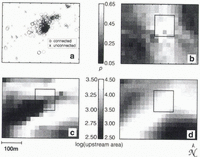
Ground-based radar data were collected on Trapridge Glacier from 1994 through 1997, providing significant areal coverage of the upper and lower basins that together represent the entire ablation zone and a fraction of the accumulation zone. Our spatial coverage is limited to safely accessible areas where a fixed survey location is visible and where the environment is conducive to high-quality sounding data. These factors preclude regularly spaced data and yield a paucity of data in regions that are heavily crevassed (e.g. icefalls) and marginal zones of very thin ice. In addition to surface coordinate survey data associated with radar transects, we collect a variety of other survey data that can be used in conjunction to map the glacier surface, including locations and elevations of a fixed glacier-wide array of velocity stakes, a mesoscale strain grid, data loggers, boreholes and longitudinal glacier profiles. These data sources together with that associated with the radar survey over the years 1994–97 yielded a total of 1700 measurements from which to reconstruct an average ice-surface map. Over the same period, 1730 radar soundings were taken which are used to reconstruct the corresponding 4 year average ice-thickness distribution. Figure 1 shows independent projections of areal coverage of ice-surface and ice-thickness (radar) data. The horizontal and vertical axes are parallel to easting and northing coordinates, respectively, and the dominant ice-flow direction is from west to cast.

Fig. 1. Areal projections of data coverage on Trapridge Glacier, 1994–97. (a) Surface-elevation survey data. Notable gaps occur coincident with an ice fall separating upper (west) and lower (east) basins, and in the southwest corner extending east along the margin where steep and crevassed terrain prohibits travel. The density of data in the centre of the ablation zone (east) is due to surveys of data loggers, boreholes and a strain grid in our study area. (b) Radar data. Gaps are coincident with those explained for ice-surface data. Regularly spaced and uniformly oriented transects are often precluded by glacier geometry and crevasses. We use data from all four years simultaneously to reconstruct average distributions of ice thickness and ice-surface elevation. The origin (southwest corner) is located at 534003E, 6787132N. North is shown as upward in this plot and is the same in those that follow unless otherwise indicated.
Instrumentation and field methods
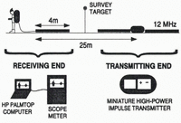
We use a high-power impulse transmitter (Reference Narod and ClarkeNarod and Clarke, 1994) in conjunction with a resistively loaded transmitting antenna of 4 m half-length, producing a centre frequency of 12 MHz. Geometry of the equipment during data collection is shown in Figure 2. The direct air wave is used to trigger the receiver, and data are transmitted via an optical cable to a battery-powered Fluke Model 97 Scopemeter. A serial interface connects the oscilloscope to an HP200LX palmtop computer that controls data collection, processing and storage.
For case of travel, antennas are oriented parallel to the propagation direction of the air wave and to the given transect. In accessible areas of the glacier, we attempt to collect continuous lines of data generally transverse to the direction of ice flow to ensure good lateral resolution. Where possible, spacing between soundings is either 12.5 or 25.0 m, with surface-elevation survey data collected less frequently (usually every 50.0 m). We implicitly assume that surface elevation gradients are smaller than basal elevation gradients so that surface coordinate data can be linearly interpolated between survey points.

Fig. 2. Geometry and components of the data-collection equipment. The transmitting end comprises the miniature high-power impulse transmitter and power supply between two antennas of 4 m half-length. Separated from the transmitter by 25 m, the receiving antenna is connected to a digital scope-meter and HP palmtop computer. The sounding location is assumed to be vertically beneath the midpoint of the two antennas, hence the position of the survey target.
Picking direct and reflected arrivals
Figure 3 shows a series of typical radar-sounding traces observed on the HP palmtop computer where the direct and reflected waves are indicated. We attempt to pick the time of the first detectable energy in the arrivals, and therefore the incidence of the wave as opposed to the peak. This strategy avoids the potential error introduced with data of variable amplitude. The results of this processing are travel times for the direct and reflected waves for each radar sounding. Ice thickness is readily computed from the travel-time difference, assuming a homogeneous ice velocity and simple parallel-planar geometry of the ice surface and bed in the vicinity of the measurement. Data migration is not necessary in this case because much of Trapridge Glacier flows unconfined over its bed; steeply dipping valley walls, usually the hallmark of glaciated terrain, are not an obvious feature of this basin. Migration techniques have been developed to handle this problem (Reference Welch, Pfeffer, Harper and HumphreyWelch and others, 1998) common to many other alpine glaciers.

Fig. 3. Example radar traces from three locations showing the direct air wave (d) and bed reflections (r). Traces A–C are presented in order of decreasing data quality and increasing uncertainty in arrival picks, demonstrating the need to quantify pick confidence in the analysis. Englacially reflected wave arrivals (e) are not uncommon in areas of complex geometry, in which case we use the signal-to-noise ratio or travel-time comparisons with neighbouring points to determine which arrival is associated with the bed.
For each radar trace, data quality is assessed and recorded by quantifying two attributes; the first pertains to the amplitude of the direct arrival, and the second to the clarity of the time-domain location of the reflected wave. The reflection index is quantitatively dependent on the number of oscilloscope pixels of uncertainly in the arrival location. Depending on oscilloscope parameters, each pixel represents the travel time through 0.68–1.36 m of ice, so an uncertainly of one pixel can introduce errors in the final ice-thickness estimates of 0.035–0.07 m. This index is thus a confidence factor for the pick that we exploit to preferentially value high-quality data in the interpolation.
Data Interpolation
The preparation we have just described yields two sets of irregularly spaced data from which we construct full arrays of interpolated data that adequately represent the whole glacier surface and ice-thickness distribution. From these, the underlying bed topography will be determined by subtraction. A variety of methods elaborated in various software is available for data interpolation; selection of a method depends on the nature of the data and a forecast of the desired outcome. Salient considerations are: whether data should be honoured exactly, how data weighting should vary with distance, and the size of the dataset. The method we adopt, kriging with prior geostatistical analysis, is relatively simple and has proven useful in a variety of other earth sciences (e.g. Reference PersicaniPersicani, 1995; Reference Piotrowski, Bartels, Salski and SchmidtPiotrowski and others, 1996; Reference Von Steiger, Webster and LehmannVon Steiger and others, 1996). The opportunity to use statistical metrics of data characterization as input in the interpolator makes this method flexible and more reliable than many other techniques that require little input other than the dataset itself.
Kriging is a linear, unbiased, least-squares interpolation procedure that uses weighted functions of spatial autocovariance to compute variable estimates. It does so by minimizing the variance of an error function, expressed in terms of kriging weights, with a Lagrangian multiplier (Reference CarrCarr, 1995). However, it requires a priori knowledge of the statistical spatial characteristics of the data as revealed in semivariogram analysis. It is unbiased because it does not shift the variable mean, nor does it change the data distribution, Kriging is an exact interpolator; therefore, it perfectly honours data at any of the specified interpolation locations, an attribute that requires spatial averaging as part of the preconditioning if conflicting data occur coincidently. Furthermore, data transformations are often necessary before kriging if spatial trends exist in the raw data. A detailed explanation and derivation of kriging weights is given by Reference CarrCarr (1995).
Data preconditioning
Because the data are relatively dense in some areas and sparse in others, we combine measurements that occur within the same 5 m gridcell. For the ice-thickness data, we compute a weighted average where each datum is favoured according to its reflection quality index. In some cases, very poor data are excluded if they are spatially redundant. For the ice-surface elevation dataset, all values are weighted equally since there is no processing step that introduces additional subjective errors.
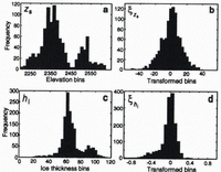
Both datasets under consideration, ice-surface elevation and ice thickness, are statistically corrupted by spatial trends that are apparent when either variable is plotted as a function of x, the easting coordinate (approximately down-flow). We anticipate spatial trends in this direction because of the ice-surface slope and the tendency for the glacier to thin toward the terminus, but in practice these trends must be empirically identified. Fortunately, in both cases the variation with x is approximately linear. To precondition the raw surface-elevation data z s , we search for a best-fit line which, when subtracted from the data, results in a mean approximately equal to zero. Let us denote the transformed surface-elevation data zs . The result of removing this trend from the data is shown in Figure 4a and b where comparative histograms of z s and zs qualitatively demonstrate that the transformed variable is normally distributed about zero.
A two-step transformation is applied to precondition the ice-thickness data. To cluster the data more effectively about a line, we first take the natural logarithm of ice thickness h i; this also ensures that the interpolation will produce positive estimates for ice thickness, because the recovered data will be the exponential of the interpolated estimate. The second step is to remove the linear trend from the logarithmic data to obtain the transformed variable hi. Figure 4c and d show histograms for the raw and final transformed data, demonstrating that the two-step transformation not only eliminates the bimodality of the original data but again yields an approximately normal distribution.

Fig. 4. Histograms of raw and transformed data. (a) Raw ice-surface elevation zs. (b) Transformed ice-surface elevation zs. (c) Raw ice thickness hi. (d) Transformed ice thickness hi. For both datasets the transformations have resulted in a data mean near zero and hare produced approximately normal distributions from bimodal raw data. The bimodal nature of distributions in (a) and (c) reflects distinct environmental and geometric factors associated with the upper and lower basins.
Geostatistical analysis
To quantify the spatial characteristics of our datasets, we use a well-known tool of geostatistical analysis, the experimental semivariogram. A variogram 2 γ(h) for a particular variable Y, considered in one dimension for simplicity, characterizes the variability between values of Y at different spatial locations (Y(x), Y(x + h)), or the autocovariance of this variable as a function of lag h (separation) (Reference Journel and HuijbregtsJournel and Huijbregts, 1978; Reference CarrCarr, 1995). Following Carr, the semivariogram γ(h) = 2 γ(h)/2 is defined mathematically as

where N is the number of data points under consideration and Y(x i +h) is the notation for a variable that is a distance h away from Y(x i ), so h = |x i+h – x i |. The semivariogram, presented here for a single variable type (Y), is a measure of similarity within the dataset and relies on the fact that similarity is inversely proportional to distance. Formally, this assumption is known as the intrinsic hypothesis and it states that variable similarity is exclusively a function of lag, not of absolute spatial location.
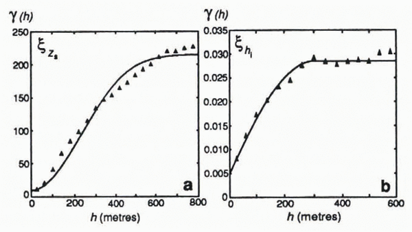
The utility of this analysis is in identifying the appropriate semivariogram model and quantifying its statistical parameters. Among the most common variogram models are those termed Gaussian and spherical. These are shown in Figure 5 along with visual explanations of their corresponding characteristic parameters. The equation of an idealized Gaussian semivariogram is (Reference Journel and HuijbregtsJournel and Huijbregts, 1978)

with γ(0) = 0 where CO, C and a are the standard representations of the statistical parameters. The “nugget” CO is the value of the semivariogram when the lag is extrapolated back to zero. Ideally CO = 0 because each data point should correlate exactly with itself, so a non-zero nugget value is indicative of random noise or spatial autocorrelation on a scale smaller than the minimum lag. Parameter C = sill – CO where the sill is defined as the constant value that γ(h) approaches at large lags and is related to the statistical variance of the data. For the Gaussian model, the “range’’ a, or transitional correlation lag, is determined by ![]() , where γ(a′) = 0.95(sill). An idealized spherical model is written as (Reference DavidDavid, 1977)
, where γ(a′) = 0.95(sill). An idealized spherical model is written as (Reference DavidDavid, 1977)

with γ(0) = 0 for CO and C as previously described, and a defined as the lag at which the semivariogram attains the sill value. For spherical models the range is determined graphically rather than computed.

Fig. 5. Two common idealized variogram models: (a) Gaussian and (b) spherical. Increasing values of γ(h) for small values of h indicate spatial correlation of the data at small lags, diminishing as separation between data pairs increases. Parameters germane to the interpolation are indicated for both models. The sill relates to the statistical variance of the data, the nugget is an indication of data errors (if it is non-zero as shown here) and the range delimits the maximum lag at which correlation is significant. The range corresponds to different values of γ in (a) and (b) because it must be uniquely calculated for each model type in order to represent the same geostatistical property.
Omnidirectional semivariograms
Semivariograms which utilize indiscriminately oriented data pairs are described as “omnidirectional”, and are the standard type. We compute omnidirectional semivariograms for datasets zs and hi using a routine provided by Reference CarrCarr (1995). These are shown in Figure 6. Visual inspection leads to the choice of a spherical model for hi and a Gaussian model for zs , which are plotted along with the experimental data. Gaussian models are indicative of data with relatively deterministic spatial variations (Reference CarrCarr, 1995), more plausible for zs than hi since zs represents a smoother and simpler surface. The parameter values used to generate the optimal semivariogram models for the data are listed in Table 1.
Directional semivariograms
Further insight into the nature of spatial autocorrelation of the data can be gained by computing directional semivariograms, which use a subset of the data chosen based on data-pair orientation. Results can reveal the imperfection of simple data transformations in removing small-scale trends, and anisotropy of the transformed data can then he quantified as a further constraint on the interpolation. We compute directional semivariograms for eight angles for each of the two datasets. As expected from the omnidirectional results, nearly all of the directional semivariograms for zs are fitted well with Gaussian models, and models for hi are unanimously spherical. The parameters that resulted from fitting models to these semivariograms are listed in Table 2 for both datasets.

Fig. 6. Experimental semivariograms (points) plotted with best-fit models (lines). (a) zs. A Gaussian model is chosen to fit this semivariogram for ice-surface elevation. (b) hi. The experimental calculation and model are plotted only for lags less than 600 m due to an insufficient number of ice-thickness data pairs at large lags. A spherical model produces the best fit to the data. Both experimental semivariograms are generated with a minimum lag of 40 m, although a choice of 20 or 60 m yields nearly identical results.
Table 1. Geostatistical parameters extracted from experimental omnidirectional semivariogram analysis of zs and hi

Of direct importance is the comparison of the ranges determined from the directional calculations, which gives the orientation and magnitude of the spatial autocorrelation anisotropy. If vectors with orientations parallel to the individual semivariogram angles, and magnitudes proportional to the corresponding ranges, are plotted with common midpoints, this anisotropy is revealed as an ellipse. From the associated angles and ranges for zs, an ellipse striking approximately northwest–southeast is definitive. It has an aspect ratio of 1.8, meaning that the range is nearly twice as great along its major axis as perpendicular to it. The directional ranges for hi vary from 150 to 375 m, and the best-fit ellipse yields an anisotropy angle of 45° west of north with a ratio of 1.4. This orientation is very close to that for zs, so residual spatial trends are similarly present in both preconditioned datasets. Having quantified the orientation and magnitude of spatial anisotropy, the required geostatistical analysis is complete, and these constraints can now be applied in the interpolation.
Table 2. Geostatistical parameters extracted from directional semivariogram analysis of zs and hi. (For a linear model, C is defined as the slope of the semivariogram)

Kriging and post-processing
A published routine (Reference CarrCarr, 1995) is used to krig both datasets with the input information discussed above, and the true recovered data obtained from the raw kriging results by reversing the transformations performed initially. All ice-thickness values are positive as a result of the logarithmic data transformation. Our kriging results are relatively insensitive to the exact values of the geostatistical input parameters but are extremely unreasonable if an unrepresentative variogram model or random parameter values are chosen. Because much of the Trapridge Glacier terminus is an ice cliff, not a gently thinning tongue, we choose to suppress information about the ice extern in the interpolation. Furthermore, introducing values of zero ice thickness into t he dataset disrupts the distribution and requires more complex data transformations. Following this approach we must artificially impose the glacier margin on the interpolated dataset, so we combine survey data and an aerial photograph to generate 25 points that adequately define its position. We then set ice-thickness values to zero that occur outside the margin and specify corresponding ice-surface elevation values equal to the local bed elevation.
Results
The results after post-processing are shown in Figure 7. Note that we have achieved the goal of producing an ice cliff at the terminus. In fact our method has produced a cliff everywhere that the ice does not extend to the grid margin, a fiction that is difficult to avoid yet not necessarily troublesome for our intended applications. Geometry of the ice and its surrounding terrain frequently prohibits visibility of our survey sites from the margin of the glacier; thus we lack data coverage where the ice is thinning, an omission which discourages marginal tapering of ice in the interpolation. Furthermore, areas of thin ice are underrepresented in the original data because reflected radar signals often occur within the tail of the direct wave, becoming indistinguishable. These interpolated datasets are constructed for use with hydrological models, and because most of the glaciologically relevant hydrological activity occurs within the interior reaches of the glacier, the marginal cliffs do not present a problem.
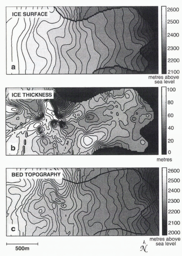
Locations of features in the interpolated datasets that have been observationally or geophysically verified are indicated by numbers in Figure 7. The ice-surface elevation is naturally smooth, and because of a lack of data in certain areas, does not well represent icefalls, although in three cases where terrain is accessible, steep slopes are recovered, as seen in Figure 7a (locations 1). The first of these areas is on the southern edge near where the ice margin extends beyond the grid; here we see a steep slope to the east. The second is the slope from the upper to the lower basin on the north side; this is an icefall that occurs as the glacier rides over a severe bedrock ridge. Upstream from this location, a third icefall is identifiable in the upper basin. Two important surface depressions (locations 2) known to store supraglacial water in summer are visible, and the prominent terminal bulges (locations 3) separated by a surface trough are successfully recovered at the eastern margin. Referencing the corresponding location on the image of bed topography (Fig. 7b), these ridges are apparent (locations 1). The steep ridge on the northern edge of the grid (location 2) does in fact crop out as such, and the overdeepened troughs behind and adjacent to it (locations 3) result in a depressed ice surface that traps surface meltwater. Ice thickness is contoured in Figure 8b along with ice-surface elevation (Fig. 8a) and bed topography (Fig. 8c). Estimates of ice thickness agree very well with measurements of borehole depths in our study area. Anomalously thick ice recovered near the southern margin has been previously identified by airborne radar measurements (personal communication from B. B. Narod, 1997), and the thinnest ice predicted at the northern margin is evident in the field as the bedrock ridge outcrops beside it.

Fig. 7. Interpolated models obtained by kriging. (a) Ice-surface elevation. The ice margin has been imposed a posteriori, rather than objectively determined by kriging, in order to enable natural estimates of bed elevation in front of the glacier terminus. Prominent features of the interpolated ice surface annotated in the text are (1) steep slopes representing icefalls, (2) surface depressions that capture supraglacial meltwater, and (3) terminal bulges at the eastern margin. (b) Basal topography. Features of the interpolated bed topography are (1) bedrock ridges, (2) a large bedrock outcrop and (3) overdeepened troughs where ice-surface depressions are observed.
Derived geometric quantities
In the simplest case, subglacial drainage might be almost exclusively controlled by geometric influences of the ice and bed. In general, this explanation is insufficient, due to the complexities of subglacial geology and varying drainage morphologies. Nevertheless, using DEMs alone, insights can be gained into the subglacial predisposition to various hydrological behaviours; this approach has been used successfully in some cases to explain experimental dye-tracing results (e.g. Reference SharpSharp and others, 1993). We refer to derived geometric quantities as those calculated solely from the interpolated datasets to distinguish them from physical model results. Two such quantities are piezometric surface (hydraulic potential) and a terrain metric called upstream area. We compute these for several hydrological situations and search tor field evidence to substantiate these results.

Fig. 8. Contoured maps interpolated by kriging. (a) Ice-surface elevation. (b) Ice thickness. Values of interpolated ice thickness are in excellent agreement with measurements of borehole depths where they are available. (c) Basal topography.
Piezometric surface
Water moves in response to potential gradients, so a useful hydrological predictor is a map of the piezometric or potential surface. Such a map cannot be constructed without knowledge of the presence and pressure of water everywhere, but one can predict water-flow paths by assuming a spatially uniform flotation fraction (P w/P i) of water pressure. In these calculations it is often assumed that the water pressure is everywhere equal to the ice-overburden pressure, perhaps an acceptable approximation for winter when an efficient subglacial drainage system is not developed. It is well established from borehole water-pressure measurements that summer meltwater can induce excursions in excess of flotation, but this condition cannot be maintained across the entire glacier bed. Therefore we consider two situations: P w = 0.5 P i and P w = P i, characteristic limits of diurnal summer water-pressure variations.
Total hydraulic potential φ is the sum of pressure potential and elevation potential (Reference ShreveShreve, 1972),
where P w is water pressure, ρ w = 1000 kg m-3 is the density of water, g = 9.81 m s-2 is the acceleration due to gravity, and z b is bed elevation. The water pressure in terms of the ice-overburden pressure is P w = f ρ i gh i, where f = P w/P i is the flotation fraction. ρ i = 917 kg m-3 is the density of ice, and h i is ice thickness. Thus we have
Figure 9 shows the results of this calculation for f = 0.5 and f = 1, visualized as contours of equal hydraulic potential. Contours that appear beyond the glacier margin are expressions of topographic potential only.

Fig. 9. Contours of equal hydraulic potential. (a) Pw/Pi = 0.5. (b) Pw/Pi = 1. Both cases are realistic for behaviours observed during the melt season. Water moves perpendicular to equipotential lines and is channeled into areas where contours are diverted to the west. Obvious outlets for water are the terminal reaches of the central and southern ice lobes. The box indicates our study area.
Both assumptions give similar results, with, f = 0.5 producing slightly more structure, a reflection of the greater influence of bed topography which varies over shorter spatial scales. Best seen for f = 1, the strongest suggestions of water channelization at the bed (indicated as contours diverted to the west) are from the upper basin into the transitional region, and near the terminus. For both f = 0.5 and f = 1, the northwest–southeast-trending potential low emerging from the upper basin appears to relieve most of the upper catchment. This potential trough continues with northern concavity into the lower basin, though it heroines much less distinct. Water flow to the glacier terminus is likely divided beneath the centre and southern ice lobes. We expect a more distributed drainage network for f = 0.5 than for f = 1 due to the slightly greater structure in its potential distribution.
Terrain analysis
Quantitative description of terrain attributes has long been used in geomorphology to characterize drainage in river basins, and is explained along with its history by Reference Zevenbergen and ThorneZevenbergen and Thorne (1987). Glaciological application of terrain analysis is not unprecedented: Reference SharpSharp and others (1993) computed upstream area distributions for Haut Glacier d’Arolla, Switzerland, based on DEMs to substantiate inferences drawn from experimental dye-tracing results; Reference Marshall, Clarke, Dyke and FisherMarshall and others (1996) have used aspects of terrain analysis to determine controls on fast-flowing ice; and Reference Bahr and PeckhamBahr and Peckham (1996) investigated the viability of describing glacier networks using statistical topology models.
For our purposes, the most relevant terrain characteristic described by Zevenbergen and Thorne is upstream area which, for a particular gridcell, is the sum of all gridcell areas that are upstream and connected. In a landscape model with known water thicknesses in each cell, computing upstream area would allow total runoff volume passing through any cell to be ascertained directly. The term “upstream” usually refers to higher topographic elevations, but to adapt this for our purposes, we use hydraulic potential differences rather than elevation gradients alone.
Much labour has gone into creating rules to calculate upstream area accurately (e.g. Reference Costa-Cabral and BurgesCosta-Cabral and Burges, 1994; Reference TarbotonTarboton, 1997). Algorithms of varying sophistication have been developed for these calculations, each attended by certain drawbacks related to grid dependence, artificial dispersion, computational memory requirements and numerical complexity. The simplest method, referred to as D8 or steepest descent (Reference TarbotonTarboton, 1997), uses a transfer rule where one gridcell gives its own area plus its upstream area to a single neighbour with the largest gradient between it and the donor. This is a numerically simple calculation but has an obvious grid bias. In a glaciological context, D8 might be useful for representing a network of discrete conduits, although it still suffers from limited flow-orientation possibilities. Reference Quinn, Beven, Chevallier and PlanchonQuinn and others (1991) improved on this by introducing a multiple-direction method that incorporates weighted area transfer where all downstream neighbours among the eight nearest receive area in proportion to relative gradients. This method largely alleviates the grid bias encountered using D8, even though only eight discrete flow directions are possible, but introduces numerical dispersion and performs poorly at boundaries. Despite this, Reference Costa-Cabral and BurgesCosta-Cabral and Burges (1994) advocate this method over the steepest-descent algorithm. A clever way of approximating continuous-flow-direction possibilities called D∞ was developed by Reference TarbotonTarboton (1997); in this approach each gridcell is divided into triangular facets, and upstream area is partitioned between two receiving cells according to the angle of steepest descent. The method performs similarly to the multiple-direction method with reduced dispersion. Tarboton’s results demonstrate this point: the drainage morphology derived from both is similar, but images resulting from D∞ calculations are sharper. In one comparative test, though, D∞ failed to reproduce proper symmetry that the multiple-direction method captured (Reference TarbotonTarboton, 1997). For our purposes, we choose the multiple-direction method as a satisfactory compromise in that it clearly outperforms D8 and is substantially easier to program than D∞. Because we are interested in qualitative drainage morphology rather than quantitative discharge calculations, this method is adequate. We have performed the same calculations using the D8 method and find that our conclusions remain unaltered, despite the fact that we believe it is an inferior representation of a hydraulically diffusive glacier bed.
Upstream area is computed for a range of flotation fractions by repeated sweeps in four directions, allowing areas to cascade down from gridcells of high potential to those of lower potential. Results for P w/P i = 0.5 and P w/P i = 1 are shown in Figure 10. DEMs with square 20 m gridcells are used in both cases. Additional tests were done with DEMs of 5 and 10 m resolution to elucidate any grid sensitivity in our method; spatial patterns obtained were visually indistinguishable in all three cases, demonstrating the robustness of this method under our working grid geometry and resolution. In describing these results, we refer to water transport and drainage patterns as interpreted from the realizations of upstream area. This terminology is justified insofar as these results represent water-flow probability distributions. We do not use terms such as discharge, which imply quantitative knowledge, since we cannot, in general, compute flow volumes; this is possible only if a constitutive equation is invoked to relate water-equivalent thickness to subglacial water pressure, a relationship which necessarily depends on the subglacial medium but is not in the spirit of the present geometrical analysis.

Fig. 10. Upstream area distributions governed by hydraulic potential. (a) Pw/Pi = 0.5. (b) Pw/Pi = 1. Plots are presented as logarithms of upstream area to remove the overwhelming downslope trend. Upstream area is possibly an indication of basin drainage morphology, or, for a particular location, a proxy for hydraulic connection probability. Bright areas represent preferential water-flow paths or areas of high connection probability. The box indicating our study area is detailed in Figure 11.
In Figure 10, brightness indicates high values of upstream area, and thus hydraulically favourable pathways in our interpretation. Results are presented as logarithms of the original calculations to remove the overwhelming downslope trend which obscures details. Shaded areas are hydraulically resistive. In the case where P w/P i = 0.5 (Fig. 10a), both ice and bed topography exert strong controls over the predicted drainage morphology. The result is a system dendritic in certain areas, diverting flow around relatively small-scale obstacles and spreading out into a uniform distribution in others. This arises because the bed is predisposed to unconfined distributed drainage, rather than channelization. One notable exception is the confluence suggested at the eastern margin where a major outlet develops, the result of a depression between the two bedrock ridges. Important to note is the discontinuity of drainage between the upper and lower basins (west and cast). The potential for ponded water is indicated by light areas surrounded by dark (hydraulic barriers). Such an area is easily visible in the upper basin where water is collected from several tributaries but flow is interrupted by prohibitive topography. These areas have potential glaciological significance as water-storage locations. Without an efficient connection between the upper and lower basins in this case, there is no obvious outlet for water entering these depressions. A further interesting feature of this upstream area distribution is the fact that no significant channelization occurs in the vicinity of the study area, suggesting distributed, inefficient flow if water pressure is low.
For the case of full flotation (P w/P i = 1), the upstream area distribution changes significantly. Water is channelized beneath the ice along a down-flow axis with a southeast excursion as it exits the upper basin avoiding a large bedrock obstacle. This axis then bends northeast back into the central area of the lower basin through the study area. Most importantly, it is the ice-surface slope that is sufficient to drive water from the overdeepened upper basin to the lower reaches of the glacier and establish the hydraulic connection that was missing at low water pressures. The qualitative differences between these two cases (high and low water pressures) is in accord with our speculations based on the hydraulic potential distributions (Fig. 9); drainage tends to be distributed and less confined at low water pressures, while high water pressures carry the influence of the ice surface and lead to more channelized morphologies. As the water enters the lower basin where bed and surface slopes are mild, the intense channelization is interrupted by two areas of distributed water. The first interruption diverts some water flow to the southern terminal lobe. This water anastomoses before converging again into a single channel that exits the glacier. The second hydraulic interruption occurs further down-flow in the centre of the basin very near our study area. Here again the flow paths eventually reconverge with a few tributaries between the bedrock ridges and emerge at the extreme end of the centre lobe. These results could be substantiated or refuted if there were subglacial outlets where water discharge could be measured, but because sediments at the margin of Trapridge Glacier are frozen, there is no observational evidence of subglacial drainage issuing from the ice-bed contact. Thus we infer that discharge generally occurs through the subsurface where it is difficult to detect.
Given the purely geometric nature of this analysis, we acknowledge that it is not generally applicable to all subglacial environments. We begin with a simple assumption (uniform water-pressure distribution) that we believe adequately represents a given hydrological state at the bed, but do not address the mechanisms that may have brought about its development. Many processes in an open system are likely to invalidate this assumption. For example, it has been shown that englacial routing can deliver large volumes of surface melt to the bed, and in some cases transport the water over significant horizontal distances before releasing it (Reference Fountain and WalderFountain and Walder, 1998); for a system where englacial transport of surface water is sufficient to maintain spatial pressure gradients at the bed, this type of analysis may be inappropriate. Furthermore, while results in Figure 10b suggest a uniaxial drainage morphology and perhaps a potential location for the development of a conduit, this analysis takes no account of detailed subglacial physics such as is appropriate for Röthlisberger or Nye channels or for canals as proposed by Reference Walder and FowlerWalder and Fowler (1994). Indeed the interaction of a subglacial water sheet and conduits would certainly preclude the possibility of sustaining uniform water pressures at the bed over short time-scales. The channel suggested in Figure 10b is 60–80 m wide and interpreted as a preferential flow path through permeable sediments rather than a channel incised in rock or ice, because the drainage of Trapridge Glacier is better characterized as a diffusive Darcian system than as a network of conduits (Reference StoneStone, 1993). In essence, this analysis is a way of isolating the hydrological effects of ice-surface and bed geometries that will undoubtedly not reflect the true complexity of the drainage network but will nevertheless modulate its development.
Despite these caveats, we attempt to predict changes in connection probability in our study area with water pressure, if upstream area can be used as an adequate proxy for this. Such behaviour has been documented at Trapridge Glacier by Reference Murray and ClarkeMurray and Clarke (1995) who identified areas of the bed that were hydraulically connected during periods of high pressure and became isolated at low pressures. We now examine our borehole-drilling records in an effort to characterize the spatial connection probability of the glacier bed.
Borehole connection record
Hot-water drilling has proceeded at Trapridge Glacier since 1980 and a log has been maintained to record drilling observations, including the connection status of each hole (whether hydraulic communication was established at the base of the glacier, indicated by a rapid drop in borehole water level). We use this information from boreholes drilled between 1989 and 1997 to construct an average connection-probability map of the study area. Figure 11a maps the borehole locations within the study area and indicates the connection status of each. From the intermingling of connected and unconnected holes, the extreme spatial and temporal heterogeneity of bed hydrology is evident. From these data we generate an interpolated connection-probability map (Fig. 11b) using the statistical kriging method we have described in this paper. For comparison with terrain analysis results, we choose 20 m gridcells; such low resolution obscures the sharp heterogeneity of Figure 11a, but indicates a region of high connection probability (bright) in the centre of the study area. This could be due to factors other than ice and bed topography, such as laterally extensive cracks near the base of the ice or continuous presence of permeable sediments.
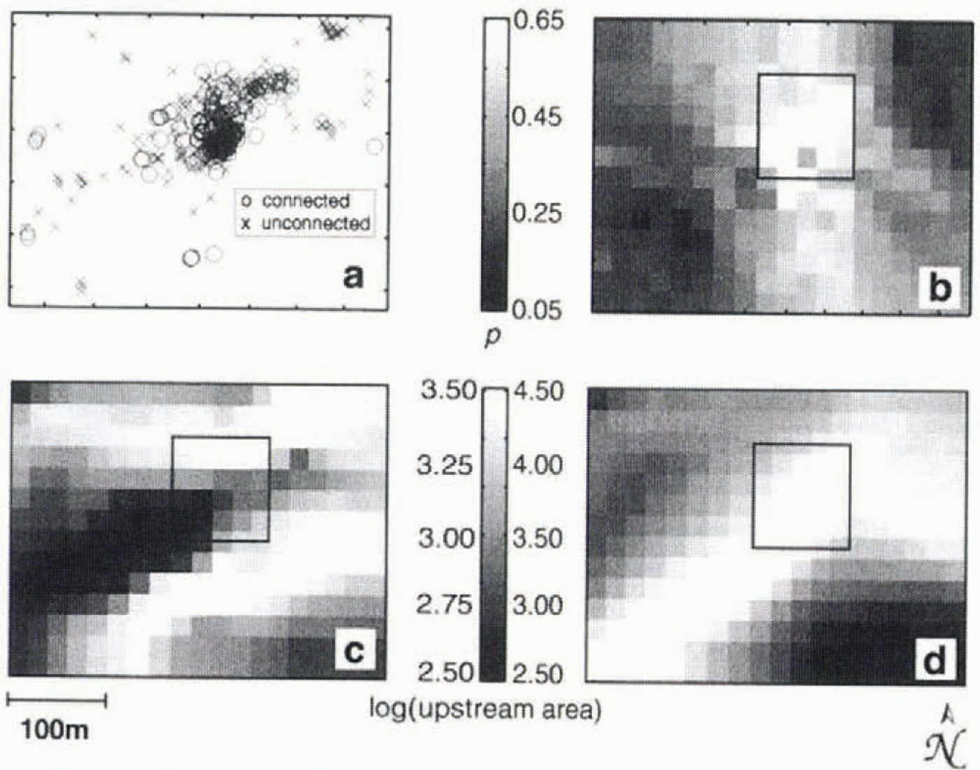
Fig. 11. Comparison of borehole connection probability and upstream area distributions for the study area. (a) Drilling observations, 1989–97, used to derive connection probabilities, (b) Connection probability distribution for 20 m gridcells obtained by kriging. The box indicates the area of highest connection probability predicted from borehole data, and appears in (c) and (d) for spatial comparison, (c) Upstream area distribution for Pw/Pi = 0.5. (d) Upstream area distribution for Pw/Pi = 1. Note the difference in shading scales in (c) and (d).
Not surprisingly, neither upstream area calculation predicts the detailed connection probability very well. Bearing in mind that the study area is the only location where we have successfully drilled connected holes on Trapridge Glacier, the fact that most of the water flow is predicted to be routed through this area (especially in the case P4w/P i = 1) is remarkable in itself. Furthermore, we note that the connection “hot spot” in the centre of the region is slightly better predicted by the upstream area distribution for P w/P i = 1 than for any other distribution resulting from P w/P i = 0.1–0.9, including P w/P i = 0.5 shown here. The difference in brightness scales in Figure 11 between panels c and d, chosen to emphasize contrasts within each panel, suppresses the evidence that the high-water-pressure regime focuses a greater fraction of the total flow through the study-area than does the low-pressure regime. Thus absolute values of upstream area in the study region and in the hot spot are much higher when P w/P i = 1. Because our drilling records are based on observations made in the midst of the melt season, it is sensible that P w/P i = 1 comes closer to capturing this feature than P w/P i = 0.5.
Concluding remarks
We have presented here a statistically reliable method for interpolating and extrapolating spatially irregular data onto a grid useful for hydrological and other models. We emphasize the importance of carefully performing the geostatistical analysis before the interpolation, and caution against uninformed use of kriging or other interpolation packages, especially in cases where constraints on the results (e.g. borehole depths) are not available. The reward for doing the statistics is the ability to provide custom information about each dataset to the interpolator, and hence obtain confident estimates of surface and bed topography.
Predictions based on derived geometric quantities afford insight into the basin-scale drainage structure of the glacier (both metrics, hydraulic potential surface and upstream area, predict preferential drainage through the study area), but are unable to account rigorously for detailed variations on scales relevant to predicting the response of borehole water-pressure transducers. Therefore, some features of the drainage clearly arise from topographic gradients of the ice and bed, but other effects such as sediment permeability and distribution must exert an equally strong influence in certain areas.
With DEMs now available for Trapridge Glacier, one new dataset is added to the small collection of complete geometric data available for alpine glaciers, which includes, among others, DEMs for South Cascade Glacier, Washington, U.S.A. (Reference Fountain and JacobelFountain and Jacobel, 1997), Haul Glacier d’Arolla (Reference SharpSharp and others, 1993), and Storglaciären, Sweden (Reference BjörnssonBjörnsson, 1981). Complete data sets are sparse despite the long scientific history of alpine glaciology, yet if accompanied by surface-velocity data, they provide important constraints for ice-flow modelling such as that undertaken by Reference BlatterBlatter (1995), O. Albrecht and H. Blatter (personal communication, 1998) and Reference Hubbard, Blatter, Nienow and MairHubbard and others (1998). Such models can make significant contributions to our understanding of stress distribution in ice and the importance of various glacier flow mechanisms. For hydrological models these DEMs are required inputs, and we have shown that geometric quantities derived from them can be used as mesoscale hydrological predictors. Detailed understanding of the hydraulic connectivity of the glacier bed and therefore of instrument signals awaits a model that includes subglacial physics. A comparison between modelled and purely geometric results should prove enlightening.
Acknowledgements
We gratefully credit D. H. D. Hildes, K. N. Foo and J. L. Kavanaugh whose contributions in the field were indispensable. We are also indebted to J. R. Carr who provided software and support for all of the geostatistical analysis and data interpolation. D. B. Bahr offered insightful suggestions on terrain analysis methods and provided useful references. Additional comments by A. G. Fountain helped clarify the manuscript. This research was funded by the Natural Sciences and Engineering Research Council of Canada. Parks Canada kindly permitted our field studies in Kluane National Park, and the Arctic Institute of North America provided a base from which to launch our fieldwork.