


Introduction
Recent observations in Greenland suggest that penetration of surface water to the bed of predominantly cold glaciers and ice sheets may accelerate the flow of these ice masses, allowing them to respond much more rapidly to climatic warming than has previously been thought (Reference Zwally, Abdalati, Herring, Larson, Saba and SteffenZwally and others, 2002). One modelling study based upon these observations suggests that, as climate warms, this effect may accelerate the contribution of the Greenland ice sheet to sea-level rise (Reference Parizek and AlleyParizek and Alley, 2004). However, the observational basis for this argument is limited, and it is possible that sustained increases in the rate of surface water input will quickly result in structural evolution of the subglacial drainage system to a morphology that reduces the sensitivity of glacier flow velocities to varying water inputs (cf. findings from temperate glaciers (e.g. Reference Nienow, Sharp and WillisNienow and others, 1998)). Subglacial drainage development therefore needs to be studied along with its effects on ice flow in predominantly cold glaciers. In this paper, we present the results from dye-tracer investigations of subglacial drainage conditions carried out over two melt seasons at John Evans Glacier, a large, predominantly cold, polythermal valley glacier situated in eastern Ellesmere Island, Nunavut, Canada (Fig. 1). The specific objectives of the research were to characterize the structure of the subglacial drainage system, to determine whether this structure evolves over a melt season, and to evaluate the impact of such evolution on the flow of the glacier.
Field Site
John Evans Glacier (79°40′ N, 74°30′ W) covers ~75% of a 220 km2 catchment, is ~15 km long, and spans an elevation range of 100-1500 m (Fig. 1). The equilibrium line is located at ~800 m (Fig. 1). Between 1997 and 2002, the mean annual air temperature at a station close to the equilibriumline altitude (ELA) (820 m) was -14.6°C. Ice is almost 400 m thick near the equilibrium line, but is typically 100-200m thick in the lower 4 km of the glacier. However, it thins to ~40 m over a large bedrock riegel ~4 km upstream from the glacier snout (Reference Copland and SharpCopland and Sharp, 2001). The average surface gradient of the glacier is low (~4.2°);two steeper sections exist at 350 m and 750 m elevation, and there is a 3 km long plateau of extremely low gradient (<0.5°) between a nunatak and the riegel (Fig. 1). The glacier consists primarily of cold ice, although the lower 4 km of the glacier is underlain by a warm basal layer which may reach up to 25 m in thickness (Reference Copland and SharpCopland and Sharp, 2001). Ice at the margins and terminus is entirely cold.

Fig. 1. Schematic map of John Evans Glacier. Note the locations of moulins h1-h5, over a bedrock riegel, and moulins h6-h7 in the accumulation zone; no other moulins are known to exist on the glacier. The supraglacial streams SS1-SS5 are composed of a series of subaerial basins connected by englacial channels; SS1 and SS3 originate in ice-marginal/supraglacial lakes L1 and L3 respectively, and SS1—SS5 terminate in h1-h5 respectively. Also marked are the locations of an automatic weather station near to the ELA; two crevasses, CL1 and CL2, which fill with water and drain englacially as the melt season progresses; two ice velocity stakes, S1 and S2, in the lower ablation zone; a geophone 200 m above the glacier terminus; and the location of a gauging station in the subglacial outflow. Although each phase of subglacial outflow occurred in a slightly different location, on the scale of the whole terminus, outflow occurred in a broadly similar location, so for simplicity the outflow is marked as a single stream emerging from the terminus.
Previous studies at John Evans Glacier (Reference Skidmore and SharpSkidmore and Sharp, 1999; Reference Copland, Sharp, Nienow and BinghamCopland and others, 2003a, b) have demonstrated that outflow of subglacial meltwater is prevented during winter by a thermal dam of cold ice at the terminus, and is restricted to a period of ~40 days during summer. Summer outflow volumes far exceed those which could be generated by basal melting alone, strongly suggesting that much of the subglacial meltwater has a supraglacial origin. The first water to emerge at the subglacial outlet each summer has a very high solute content and may consist of ‘old’ waters that have been stored over winter in a subglacial reservoir. As outflow continues, these ‘old’ waters become progressively diluted, most likely by new inputs of surface meltwater (Reference Skidmore and SharpSkidmore and Sharp, 1999; Reference HeppenstallHeppenstall, 2001). Five moulins, h1-h5, located in a crevasse field over the riegel (Fig. 1), have been proposed as the likely access points to the subglacial system for supraglacial meltwater (Reference Skidmore and SharpSkidmore and Sharp, 1999). These moulins form the termini of five large supraglacial streams, SS1-SS5, which flow across the low-gradient plateau between the nunatak and the riegel (Fig. 1). Reference Boon and SharpBoon and Sharp (2003) described the processes involved in the seasonal initiation of inflow to these moulins.
Methods
Dye-tracer experiments
Fieldwork was conducted from 1 June to 3 August 2000 and from 21 May to 1 August 2001. During each melt season, followingthe onset of subglacial outflow, known quantities of the fluorescent dye rhodamine WTwere injected periodically into moulins h1-h5. Injections were typically undertaken at or within an hour of 1400 h at h1 but, on occasions in mid- July 2000, injections were made instead into h2, h3 and h4. Towards the end of each melt season (30 July 2000, 28 July 2001), dye was injected into an additional moulin, h6, at 915 m elevation, which was not active earlier in the season. Immediately prior to each dye injection, the discharge, Q S, of the supraglacial stream flowing into the moulin was measured using the velocity-area method (e.g. Dackcombe and Gardiner, 1983). The mean of five flow-velocity measurements was used to derive Q S, and maximum and minimum estimates of Q S were derived from the maximum and minimum measured flow velocities respectively.
Dye emergence at the glacier snout was monitored by fluorometric analysis of water samples collected from the gauging station at the subglacial outflow (Fig. 1) at intervals of 5 min to 1 hour using an automatic pump sampler. Sampling started before measurable concentrations of dye were recorded, and ceased when all available sample bottles (up to a maximum of 72) had been used. Where possible, sampling frequency was increased as the dye concentration peak arrived at the subglacial outflow and was decreased during the tail of the dye return curve (after Reference SmartSmart, 1988). Continuous-flow fluorometry could not be used to monitor dye emergence because the suspended sediment fluoresced at the same wavelength as the dye. Suspended sediment was therefore removed from the water samples by sedimentation over 24hours prior to fluoro- metric analysis.
Five parameters were determined from the dye-breakthrough curves (after Reference Nienow, Sharp and WillisNienow and others, 1998):
The dye transit time, t, which is the period between dye injection and peak dye concentration at the detection point.
A minimum estimate of the mean water-flow velocity, u, given by u = x/t, where x is the distance between the injection and detection sites, assuming flow parallel to the glacier margins.
The dispersion coefficient, D (m2s-1), which describes the rate of spread of the dye cloud during its passage through the glacier (Reference Seaberg, Seaberg, Hooke and WibergSeaberg and others, 1988, equation 4, p. 222).
The dispersivity, d, which describes the rate of dispersion of the dye cloud relative to its rate of advection through the glacier, and provides a characteristic length scale for the system (Reference FischerFischer, 1968). This is given by d = D/u (after Reference BrugmanBrugman, 1986).
An estimate of the mean cross-sectional area, A M, of the subglacial drainage system between h1 and the subglacial outflow, determined by A M = Q S/u, where Q S is the discharge entering moulin h1 (after Reference Willis, Sharp and RichardsWillis and others, 1990; Reference Hock and HookeHock and Hooke, 1993). Because discharge increases between h1 and the subglacial outflow, this method is likely to underestimate the mean crosssectional area of the subglacial drainage system, so values of A M provide an index, rather than a true measure, of cross-sectional area.
Due to the discrete nature of the sampling, the water samples may not have captured the true peak in dye concentration. Hence, an average value of t for each dye experiment was determined using the apparent peak from each breakthrough curve, and minimum t and maximum t were estimated by considering the times at which water samples were collected on either side of the apparent peak. Errors in u, d and A M were derived by considering maximum and minimum values of t and, where necessary, Q S in each calculation.
Supplementary hydrological measurements
Discharge into and out of the subglacial drainage system were monitored during both melt seasons to assess whether seasonal changes in the parameters (derived from the dye traces) were attributable to changes in subglacial hydraulic structure and/or discharge (either supraglacial discharge, Q S; bulk subglacial discharge, Q B; or both). To obtain a record of Q S, a pressure transducer was used to monitor stage in SS1, which drained into h1 (Fig. 1). These measurements were converted to Q S using a stage-discharge rating curve covering the full range of water levels in SS1. Since SS1 is only one of five supraglacial streams draining into the glacier over the riegel, this estimate of Q S serves as an index of supraglacial inputs to the glacier. Attempts to record Q B using a pressure transducer to monitor stage in the subglacial outflow were unsuccessful owing to frequent channel aggradation and migration. As a result, variations in subglacial discharge had to be assessed qualitatively on the basis of regular observations of the subglacial outflow and occasional discrete manual measurements of Q B. Throughout each melt season, the electrical conductivity (EC) of the subglacial outflow was measured at 15 min intervals, and the hourly average air temperature was measured at an automatic weather station located near to the ELA (820m;Fig. 1).
Surveys of ice motion
To determine temporal variations in the rate of glacier flow, the positions of 33 prisms mounted on stakes drilled and frozen into the ice throughout the lower 3 km of the glacier were measured every 2 days, weather permitting, using an electronic total station. Some of the results from this study are presented in Reference Bingham, Nienow and SharpBingham and others (2003). Selected data are presented here to allow comparison with results from the dye-tracer tests. Glacioseismic activity was monitored using a 4.5 Hz geophone, drilled 3 m into the ice surface at a site ~-200m up-glacier from the glacier -logger which counted the number of seismic events above a given threshold (with a gain of 2000) and output a sum every 2 hours (after Reference Copland, Sharp, Nienow and BinghamCopland and others, 2003b). The aim was to detect seismic activity associated with enhanced ice-motion events and/or fracture of cold ice near the snout (e.g. Reference Raymond, Benedict, Harrison, Echelmeyer and SturmRaymond and others, 1995; Reference Kavanaugh and ClarkeKavanaugh and Clarke, 2001).
Results
Hydrological observations
Opening of moulins and onset of subglacial outflow
In 2000, supraglacial drainage into h1-h5 began between the afternoon of 19 June, when h1-h5 were still sealed and surface ponding was occurring along supraglacial streams SS1-SS5 (Fig. 1), and midday on 21 June. Subglacial outflow started on the afternoon of 22 June as a turbid upwelling ~1 m in front of the glacier snout (at the ‘gauging station’, Fig. 1). Over the next 4days the upwelling migrated headwards and evolved into a channel, incised upwards into the ice, which persisted for the remainder of the melt season with varying discharge. In the accumulation zone, moulins h6 and h7 opened some time between 5 and 19 July and captured streams which had previously drained supra- glacially to the ice margin. In addition, two large water-filled crevasses, CL1 and CL2 (combined storage >10 000 m3), located 500 m up-glacier from the nunatak (Fig. 1), drained entirely in <2 hours on 20 July and 1 August respectively.
In 2001, h1-h5 opened on 28-29 June, and subglacial outflow started at 1215 h on 29 June ~50 m to the east of the now-sealed outlet portal from 2000. The subglacial discharge diminished and almost ceased during the 2 weeks following the outburst. Outflow then increased significantly on 15 July and ~2-3 further upwellings developed ~15 m to the east of the initial 2001 outlets. This 15 July event is hereafter termed the ‘secondary outburst’. By 17 July, all subglacial discharge drained from the easternmost outlet, and it persisted at that site for the remainder of the melt season with a discharge that varied diurnally. Moulins h6 and h7 opened some time between 13 and 21 July, but CL1 and CL2 had not drained when the field season ended on 1 August. Thus, the number of locations where surface water entered the glacier varied between years and, in each year, surface-water inputs tended to be initiated later in the season at points further up-glacier.
Discharge records
Supraglacial discharge, Q S, records from SS1 are presented in Figure 2a and b, together with records of air temperature (Fig. 2c and d) and EC (Fig. 2e and f). Calibration problems led to underestimation of Q S at times of exceptionally high discharge, so more realistic (qualitative) estimates for these periods (based on tidemarks created during each event) are suggested in Figure 2a and b. In view of these problems, we regard the seasonal records of Q S as indices of inflow rather than absolute values. Only those values of Q S that were measured directly at the time of dye injections were used in analyses of the dye-tracer results.

Fig. 2. Fig. 2. (a, b) Record of supraglacial discharge, Q S, draining into h1 during summer 2000 (a) and 2001 (b), based on a correlation between continuous stage records obtained by a pressure transducer ~300m upstream of h1 (Fig. 1) and discrete discharge measurements made at h1. Qualitative estimates of Q S, based on peak tidelines, are shown for periods when stage rose well above the sensitivity of the transducer. (c, d) Mean daily air temperatures measured near the ELA (820 m) in summer 2000 (c) and 2001 (d). (e, f) Record of electrical conductivity, EC, measured in the subglacial outflow during 2000 (e) and 2001 (f). Gaps occur where the subglacial outflow migrated away from the gauging station and manual samples were not collected. Manually sampled values added for the period 29 June-3 July 2001.
Qualitative observations and discrete measurements of bulk subglacial discharge, Q B, suggest that changes in Q B largely reflected variations in Q S throughout both melt seasons. For example, in 2000 Q B oscillated diurnally between ~1 and 4 m3s-1 from 26 June to 23 July. By contrast, in 2001 Q B remained very low after the initial subglacial outburst, rarely exceeding 1 m3 s-1 until the secondary outburst on 15 July, after which it is estimated Qb varied diurnally between ~5 and 10m3s-1. The record of Q S may therefore provide insight into the temporal pattern of variations in Q B in both melt seasons. There was, however, one notable exception to this. On 24 July 2000, Qb increased by an estimated ~4-5m3s_1, and thereafter stayed high (>4 m3 s-1), oscillating diurnally, until the end of the field season. This stepped increase in Q B is not mirrored in the Q S record (Fig. 2a), and may reflect the arrival at the glacier terminus of water that entered the glacier at moulins h6 and h7. After 24 July, however, diurnal oscillations in Q B continued to lag diurnal oscillations in Q S. During the extreme melt event of 28-30 July, peak Q B was estimated to reach ~30 m3 s-1 (Reference Boon, Sharp and NienowBoon and others, 2003).
Ice surface velocities
Figure 3 shows the horizontal and vertical speeds of two marker stakes, S1 and S2, which are representative of broad- scale patterns of ice flow in the 4 km long section of the glacier between the bedrock riegel and the terminus (Fig. 1). These records show increased horizontal and vertical (upward) velocities between 21 and 27 June 2000 (Fig. 3a and b) and 26 and 29 June 2001 (Fig. 3c and d). In both years, these periods of increased velocity coincided with high levels of seismic activity recorded by the geophone above the glacier terminus (Fig. 3e and f). In 2001, a second period of increased horizontal and upward vertical velocities occurred in this area between 15 and 17 July (Fig. 3c and d).

Fig. 3. Fig. 3. (a-d) Time series of horizontal (thick lines) and vertical (thin lines) speeds at ice motion stakes S1 (a, c) and S2 (b, d) in summer 2000 (a, b) and 2001 (c, d). Mean annual horizontal speeds (dashed) and zero vertical uplift (dotted) are also shown. Derivation of errors is discussed in Reference Bingham, Nienow and SharpBingham and others (2003). (e, f) Seismic activity recorded during 2000 (e) and 2001 (f) at a geophone drilled into the ice surface ~200m above the glacier terminus. The grey boxes highlight high-velocity events as follows: event 1/00 was associated with the initiation of subglacial outflow in 2000, event 1/01 relates to the onset of subglacial outflow in 2001 and event 2/01 coincided with a secondary outburst on 15 July 2001.
Dye-tracing experiments
Breakthrough curve characteristics: 2000 melt season
All dye-breakthrough curves recorded in 2000 were characteristically asymmetrical in form, with a sharp rise to peak concentrations and an elongated tail (Fig. 4a). Dye injected into h1 shortly after the initiation of drainage into h1-h5 on 25 June had a mean flow velocity, u, of 0.14 m s-1 (Fig. 4b). Subsequently, u increased as the melt season progressed, reaching 0.46 ms-1 on 8 July and 0.69 ms-1 on 28 July (although a reversal of this trend was observed on 11 July, when u fell to 0.14 m s-1) (Fig. 4b). At the same time, with the exception of the 11 July injection, breakthrough curves became progressively less dispersed as the melt season progressed (Fig. 4a). This is reflected in a general decline in dispersivity from 114m on 25 June to 19m on 28 July (Fig. 4c). The index of mean drainage cross-sectional area, A M, declined from 6.0 to ~1 m2 during the early melt season (25 June-6 July) and remained low thereafter (Fig. 4d).

Fig. 4. Sequence of breakthrough curves derived from injections made into h1 during 2000. (b_d) Temporal variations in (b) mean water flow velocity, u, (c) dispersivity, d, and (d) apparent subglacial channel cross-sectional area, A M, for dye-tracer tests carried out from h1 during summer 2000 (solid lines). Information from single injections made into h2, h3 and h4 in 2000 is also shown in (b) and (c). (e_h) Equivalent records from summer 2001. Note the difference in x-scales between (a) and (e).
Dye injected into moulin h6 on 30 July 2000 produced a dispersed return curve with a mean flow velocity of 0.24 m s-1 and dispersivity of 250 m. The curve had multiple peaks on its rising and falling limbs (Fig. 5).
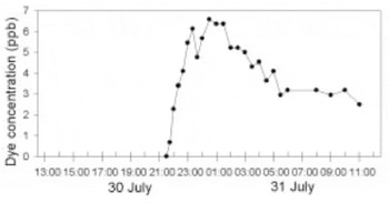
Fig. 5. Dye-breakthrough curve obtained from a single injection into h6 at 1230 h on 30 July 2000.
Breakthrough curve characteristics: 2001 melt season
From 1 to 14 July 2001, dye-breakthrough curves were highly dispersed, with multiple peaks (Fig. 4e). By contrast, injections on 19 and 22 July yielded highly peaked return curves (Fig. 4e). The first dye test on 1 July gave u = 0.05 ms-1, and subsequent injections between then and 14 July yielded similar velocities. Thereafter, u increased to 0.27 ms-1 by 22 July (Fig. 4f).
The decline in the spread of the dye curves after 8 July (Fig. 4e) is reflected in a general seasonal decrease in dispersivity (Fig. 4g). The value of A M decreased between 1 and 4 July, but increased again between 8 and 14 July, before decreasing from 7.6 to 5.4 m2 between 14 and 22 July (Fig. 4h). Dye injected into h6 on 28 July 2001 was not detected in the subglacial outflow.
Interpretation and Discussion
Variation of throughflow velocity with discharge
In order to determine whether the observed variations in u (Fig. 4b and f) resulted from changes in subglacial drainage system structure or solely from variations in discharge, Q, through the system, it is necessary to examine whether the relationship between u and Q changes significantly with time in each summer. Regardless of whether subglacial water flow occurs in full or partially full conduits, u will be directly proportional to Q so long as the subglacial drainage system structure remains unchanged (Reference Nienow, Sharp and WillisNienow and others, 1996). If, however, the form of the u to Q relationship changes significantly during the course of a melt season, this may be interpreted as evidence of a changing subglacial drainage system structure. Since a continuous record of Q B does not exist, values of Q S were used here as a proxy for variations in Q throughout the subglacial drainage system. Several previous studies have demonstrated that u may be more closely related to Q S than to Q B (Reference Behrens, Bergmann, Moser, Ambach and JochumBehrens and others, 1975; Reference Nienow, Sharp and WillisNienow and others, 1996).
In the early phase of drainage into h1 in 2000 (25 June- 6 July), u remained consistently low despite large variations in Q S (Fig. 6). This suggests that, early in the melt season, discharge variations were accommodated by relatively large changes in the cross-sectional area of the subglacial drainage system. However, from 8 to 28 July 2000 u and Q S were significantly related (u =0.83QS 09; r 2 = 0.82). We interpret this relation as evidence that, after 8 July, changes in u were caused mainly by changes in Q S rather than by changes in A, suggesting a relatively stable subglacial drainage system structure. This is consistent with the behaviour of the A M index in 2000 (Fig. 4d), which suggests that the drainage system cross-sectional area changed little between 8 and 28 July 2000.

Fig. 6. Variation of mean water velocity, u, with supraglacial discharge, Q S, into h1 during 2000 (thin black line) and 2001 (dotted line). Thick black lines denote trend lines for 8_28 July 2000 and 1_22 July 2001 as discussed in text.
The u-QS relationship in 2001 (Fig. 6) is more difficult to interpret. Taken at face value, u and Q S appear to be significantly related (u = 0.15 Q S 07; r 2 = 0.91) throughout the melt season. However, because u and Q S were so low and constant from 1 to 14 July, but then rose significantly from 14 to 19 July (Fig. 6), the relationship essentially reflects the contrast between traces conducted between 1 and 14 July and those conducted between 19 and 22 July. Hence, it is doubtful whether the derived relationship is applicable to either period in 2001. Instead, we suggest that throughout the 2001 melt season, u was much less sensitive to Q S than in July 2000, and in 2001 drainage-system crosssectional area always played a significant role in the response of the system to varying discharge. This is supported by the fact that A M remained larger throughout 2001 than in 2000, indicating limited subglacial channel development in the later season (Fig. 4d and h).
2000 melt season: hydrological development
Onset of englacial drainage and subglacial outflow
The sudden drainage of surface meltwater ponded along SS1-SS5 into h1-h5 on 19-21 June probably occurred in response to the rapid downward propagation of water-filled crevasses through cold ice over the bedrock riegel (Weert- Reference Weertmanman, 1973; Reference Scambos, Hulbe, Fahnestock and BohlanderScambos and others, 2000; Reference Boon and SharpBoon and Sharp, 2003). At this time, water levels in the crevasses over the riegel, and in the surface ponds overlying the crevasses, far exceeded the threshold that Reference Scambos, Hulbe, Fahnestock and BohlanderScambos and others (2000, equations 5-7) suggest is required for crevasse propagation to the glacier bed. The occurrence of hydrofracture is also suggested by audible ice-quake activity over the riegel at this time. The exact points at which the englacial and subglacial systems connect are unknown. However, the widespread surface-velocity response to this drainage event throughout the lower 5 km of the glacier (Fig. 3a and b) indicates that the water draining into h1-h5 rapidly accessed the glacier bed in the vicinity of the riegel, inducing high subglacial water pressure throughout the lower ablation zone. Multiple premonitory drainage events in the 1-2 days before h1-h5 opened fully (e.g. Reference Boon and SharpBoon and Sharp, 2003) may explain why velocities at S2 began to increase before 19 June (Fig. 3b).
The sudden drainage of meltwater into moulins h1-h5 between 19 and 21 June was instrumental in the initiation of subglacial outflow at the terminus on 22 June. Rapidly induced high water pressure in the subglacial reservoir behind the thermal dam at the terminus presumably caused subglacial meltwater to force a path through cold ice and/or frozen sediments into the proglacial zone (cf. Reference Skidmore and SharpSkidmore and Sharp, 1999). Hydrofracture may have played a role in the process of dam breaching, which was accompanied by heightened seismic activity 200 m above the terminus (Fig. 3e) and the emergence of turbid, solute-rich water from small, freshly formed crevasses on the glacier surface ~300 m up-glacier of the snout. The first water to emerge in the outflow had very high EC (>0.035 S m-1; Fig. 2e), suggesting release from long-term (possibly overwinter) storage at the glacier bed. The subsequent decline in EC, followed by the onset of diurnal variability on 26 June (Fig. 2e), probably reflects dilution of the subglacial reservoir by new surface meltwater inputs.
Subglacial drainage evolution
On the basis of the u-Q S relationship (Fig. 6) and the behaviour of the A M index (Fig. 4d), the period of subglacial outflow during 2000 may be divided into two distinct periods: a period of subglacial drainage system evolution (25 June-8 July) and a period of subglacial drainage system stability (8-28 July). During the first period, u increased gradually despite declining Q S (Fig. 6), and A M declined progressively (Fig. 4d), apparently reflecting a period of structural evolution (formation of channels) of the englacial and/or subglacial drainage system. During the second period, from 8 to 28 July, u and Q S were quasi-linearly related (Fig. 6) and A M remained constant and low (Fig. 4d). These trends suggest that channel formation in the drainage system between h1 and the terminus was complete by 8 July and that subsequent changes in u were primarily indicative of fluctuating subglacial discharges in a hydraulically efficient channelled system characterized by low total cross-sectional area.
The behaviours of u and d in relation to A M (Fig. 4b-d) further support the proposed subdivision of the 2000 melt season. Low u, and high d and A M on 25 June (~3 days after h1-h5 first opened and subglacial outflow began) reflect an inefficient, distributed subglacial network. By 29 June, a rise in u and drop in A M imply that flow was then taking place through a developing channel. Channel formation was initially driven by the rapid drainage of supraglacially stored meltwater into h1-h5, and by the drainage along the streams draining into these moulins of ice-marginal lakes L1 and L3 (Fig. 1), on 24-25 June and 23-24 June respectively. After 26 June, by which time all supraglacial stores connected to SS1-SS5 had effectively drained, the continued development of subglacial channels was dependent upon melt- induced surface runoff into h1-h5. Over the first few days of channel development, it is unlikely that channel growth could keep pace with meltwater inputs, leading to the partial migration of meltwater into the pre-existing distributed system and a consequent increase in d on 29 June (Fig. 4c). The continued decline in A M, rise in u and decrease in d until 8 July (Fig. 4b-d), together with the slowing of surface ice-flow velocities after 27 June (Fig. 3a and b), suggest that the subglacial network became increasingly channelled by ~8 July as high air temperatures (Fig. 2c) maintained consistently high rates of surface melting (Fig. 2a).
From 8 July until the end of the melt season, all hydrological indicators suggest that drainage between h1 and the subglacial outflow took place through a relatively stable, hydraulically efficient, channelled system. Throughout this period, A M remained stable (Fig. 4d) and variations in u and d (Fig. 4b and c) probably resulted almost entirely from changes in discharge through the subglacial system (Fig. 6). Generally high u and low d from 8 to 28 July (Fig. 4b and c) reflect continued high supraglacial meltwater inputs (Fig. 2a). The only exception occurred on 11 July, when low u and high d (Fig. 4b and c) resulted from low Q S (Fig. 2a) during a brief cool spell (Fig. 2b), suggesting that, during this period of low meltwater input, hydromechanical dispersion increased in importance relative to advection as low fluxes of meltwater passed slowly through large subglacial channels.
Continued diurnal variations in EC in the subglacial outflow (Fig. 2e) from 8 July to 2 August further support the maintenance of an efficient channelled subglacial network beneath the lower ablation zone throughout the latter part of the 2000 melt season. That the majority of the water was draining subglacially, rather than englacially, is indicated by consistently high EC in the subglacial outflow (~0.02 S m-1, Fig. 2e) relative to typical supraglacial values (<0.001 S m-1; Reference HeppenstallHeppenstall, 2001).
Spatial expansion of subglacial drainage
The onset of englacial drainage at moulins h6 and h7 between 5 and 19 July, and the demonstrated connection between h6 and the subglacial outflow, signal an up-glacier expansion of the englacial and/or subglacial drainage system in late summer 2000. One possible explanation for the extremely high values of D (60 m2s-1) and d (250 m) obtained from the 30 July experiment is that dye flowed initially through a distributed drainage system and then into an efficient channelled system as it travelled down-glacier (cf. Reference Nienow, Sharp and WillisNienow and others, 1998). If we assume that meltwater draining into h6 on 30 July flowed orthogonal to contours of equal subglacial hydraulic potential and intersected the channelled system immediately below h1, and that the h1-to-outflow velocity on 30 July ranged from 0.51 to 0.68 ms-1 (as between 1100 and 1700 h on 28 July), water would have travelled between h6 and h1 at 0.15-0.16 m s-1. This velocity range is consistent with meltwater travelling through a relatively inefficient distributed system from h6/h7 to the riegel, before intersecting a channelled network in the lower 4 km of the glacier. The initial passage of dye through a distributed system in the upper glacier would also explain many of the peaks/shoulders on the return curve (Fig. 5), as dye may have flowed through a series of links (cf. Reference KambKamb, 1987) or anabranches in a distributed network prior to intersecting an efficient channel, or channels, beneath the lower ablation zone. Whilst the precise timing of the onset of drainage into h6/h7 remains unclear, the sudden increase in Q b on 24 July, followed by consistently high (but still diurnally fluctuating) Q B until the end of the melt season, may indicate the date of connection. Additional meltwater entering the drainage system in the accumulation zone via sudden drainage of CL1 on 20 July may have helped to drive this connection, and drainage of CL2 on 1 August probably supplemented these inputs towards the end of the melt season. This spatial expansion of subglacial drainage may have caused seasonal variations in basal motion as far up-glacier as the mid-accumulation zone (Reference Bingham, Nienow and SharpBingham and others, 2003).
2001 melt season: comparison with 2000
Until the subglacial outburst on 29 June 2001, the evolution of the hydrological system and the surface dynamic response at John Evans Glacier paralleled that seen in 2000, but after 29 June the hydrological behaviour differed significantly. On 28 June (coinciding with the onset of drainage into h1-h5), a prolonged period of low temperatures (<2°C) and intermittent snowfall began, and this persisted until 12 July (Fig. 2d). Over this period, surface runoff was very low and, once supraglacially stored water along SS1-SS5 (including L1 and L3) had drained into h1-h5, meltwater input to the subglacial drainage system dropped dramatically (Fig. 2b). Consequently, little or no evolution of the subglacial drainage system took place in the first 2 weeks after the subglacial outburst, as indicated by consistently low u (<0.07ms-1, Fig. 4f) and multiple-peaked return curves between 1 and 14 July (Fig. 4e), which suggest that dye was travelling through a hydraulically inefficient subglacial drainage system. The maintenance of very high (albeit diurnally fluctuating) EC in the subglacial outflow until 12 July (Fig. 2f) further supports the probable predominance of distributed subglacial drainage, solute acquisition being enhanced by long residence times and access to large areas of the glacier bed (Reference TranterTranter and others, 1997). The variation in Am from 1 to 14 July (Fig. 4h) is best explained by changes in discharge through the system (Fig. 2b), with low values of Am and u on 4 and 8 July (Fig. 4f and h) reflecting low discharge through the subglacial system rather than any rationalization (or channel formation) of the drainage configuration.
From 12 July until observations ceased (1 August), clear skies and high temperatures (Fig. 2d) resulted in significant surface runoff and increased discharges into h1-h5 (Fig. 2b). Enhanced horizontal surface speeds and surface uplift, associated with audible ice-quake activity, and the occurrence of the secondary outburst from the terminus on 15 July, suggest that renewed surface inputs to the subglacial system generated high basal water pressures in a network which had remained largely distributed since the initial outburst at the end of June. After 13 July, EC began to fall significantly (much as it did after the initial outburst in 2000;cf. Fig. 2e and f), and after 14 July, u rose whilst A M and d dropped (Fig. 4f-h), suggesting that with sustained surface inputs to h1-h5, subglacial channel formation was then taking place. The behaviour of the subglacial drainage system from ~12 to 25 July 2001 thus mirrored that from 22 June to 6 July 2000, indicating that late July 2001, like late June to early July 2000, was a period of structural evolution of the subglacial drainage system driven by sustained and large inputs of surface runoff. However, by 22 July the subglacial drainage system was still considerably less efficient than at the same stage of the previous melt season, reflecting the more limited time available for supraglacially driven channel formation in the subglacial drainage system.
The lengthy cool period in early July 2001 may also have led to more limited up-glacier expansion of the en/sub- glacial drainage system. Although h6 and h7 opened between 13 and 21 July, dye injected into h6 on 28 July was not detected in the subglacial outflow. Zero dye recovery could indicate that: (i) dye became so dispersed that it emerged in the subglacial outflow below detectable levels; (ii) dye was delayed in the system up-glacier of the riegel, and subsequently emerged after the observation period; or (iii) no connection was made between meltwaters draining into h6 and h7 and the subglacial network downstream of the riegel. Irrespective of the cause, the result suggests that the drainage system up-glacier from the riegel was less hydraulically efficient in late July 2001 than at the same stage in 2000.
Implications for High Arctic glacier response to climate change
The findings reported here have a number of significant implications for the potential response of predominantly cold glaciers to climatic warming. Firstly, the rapid formation of channels within the subglacial drainage system observed at John Evans Glacier contradicts Reference Rabus and EchelmeyerRabus and Echelmeyer’s (1997) suggestion that subglacial drainage systems in such glaciers will be poorly developed, and instead implies that they can evolve rapidly in response to seasonal inputs of supraglacially derived meltwater. Where surface melt can penetrate to the base, it will induce a surface velocity perturbation as observed here, and thereby enhance annual rates of mass transfer to lower elevations and accelerate annual rates of surface melting and runoff. However, rapid formation of channels as recorded here will significantly check the overall increase, because once the subglacial system becomes hydraulically efficient, the surface velocity response to supraglacial hydrological forcing is significantly dampened. This may contrast with the situation reported for the Greenland ice sheet (Reference Zwally, Abdalati, Herring, Larson, Saba and SteffenZwally and others, 2002), where channel formation is restricted by large overburden pressures and the surface velocity response to the penetration of surface water to the bed may be prolonged.
A second significant finding of this study is that, although there may be multiple points where surface water can reach the bed of a High Arctic glacier, not all will necessarily be active in any given season. Hence, in a warmer summer (2000), the length of the glacier segment affected by penetration of surface waters to the base was greater than in a cooler summer (2001), and this has significant implications for the proportions of the glacier affected by surface- melt-induced velocity perturbations. Hence, with a trend towards warmer summers at high latitudes (Reference HoughtonHoughton and others, 2001), and a consequent rise in ELAs, greater proportions of High Arctic glaciers are likely to experience supraglacially forced basal motion and subglacial drainage evolution. However, given the rapidity with which channel formation occurs after moulins become active, surface velocity perturbations in response to supraglacial meltwater penetration to the basal interface are likely to be less pronounced than on the Greenland ice sheet.
Conclusions
Dye-tracing experiments conducted at John Evans Glacier during two melt seasons (2000, 2001) demonstrate that the configuration of the subglacial drainage system of this large, predominantly cold polythermal glacier can evolve significantly as the melt season advances. Each melt season, subglacial outflow and early subglacial drainage system evolution are induced by the drainage of large volumes of stored supraglacial meltwater to the glacier base. Subsequently, subglacial drainage system evolution is controlled directly by rates of surface melt-derived runoff. When high rates of surface melting are sustained (e.g. 2000), the basal drainage system evolves rapidly into a hydraulically efficient channelled configuration. When surface melting is limited for a sustained period following the supraglacially driven outburst event (e.g. 2001), basal drainage may remain predominantly distributed for much of the melt season. In warmer years (e.g. 2000), the area of the bed that drains supraglacially derived meltwaters expands upstream in response to the capture of surface streams by moulins and crevasses which open in the accumulation zone.
Supraglacially driven hydrological forcing and subglacial drainage evolution as observed at John Evans Glacier demonstrably impact upon glacier dynamics, and may thus account for intra-annual variations in surface velocities that have been observed at glaciers with comparable thermal regimes (Reference Müller and IkenMüller and Iken, 1973; Reference WillisWillis, 1995; Reference Rabus and EchelmeyerRabus and Echelmeyer, 1997). However, at John Evans Glacier rapid channel formation within the subglacial drainage system limits the period over which supraglacial hydrological forcing enhances basal motion. As a result, the coupling between subglacial hydrology and glacier dynamics may play a less important role in the response of cold High Arctic glaciers to climate warming than it does in the response of the Greenland ice sheet (cf. Reference Zwally, Abdalati, Herring, Larson, Saba and SteffenZwally and others, 2002).
Acknowledgements
Financial support was provided by the UK Natural Environment Research Council (NERC) ARCICE Thematic Programme (grant GST/02/2202;P.W.N.) with tied NERC studentship (24/99/ARCI/16;R.G.B.);an NSERC Discovery Grant (155194-99;M.J.S.);a Natural Sciences and Engineering Research Council (NSERC, Canada) scholarship (PGSA-232321;S.B.);University of Alberta Canadian Circumpolar Institute C/BAR grants; and grants from the Geological Society of America and the Northern Science Training Program. Invaluable field support and logistics were provided by the Canadian Polar Continental Shelf Project; this is PCSP contribution No. 00405. We gratefully acknowledge J. Barker, K. Heppenstall, D. Lewis and T. Wohlleben for field assistance, and thank the Nunavut Research Institute and the communities of Grise Fjord and Resolute Bay for permission to work at John Evans Glacier. We also thank T. Creyts and U. Fischer for insightful reviews, and J. Walder and T.H. Jacka for constructive editorial work on the manuscript.


