


1. INTRODUCTION
Natural granular flows such as soil liquefaction, debris flows and snow avalanches cause damage to property and lead to loss of human life (Armstrong and others, Reference Armstrong, Williams and Armstrong1992). Such types of flows frequently impact on obstructions as they stream down an inclined surface, producing fast changes in flow height and velocity in their neighbouring region (e.g. Savage, Reference Savage1979; Tai and others, Reference Tai, Gray, Hutter and Noelle2001; Gray and others, Reference Gray, Tai and Noelle2003; Hakonardottir and Hogg, Reference Hakonardottir and Hogg2005; Cui and others, Reference Cui, Gray and Johannesson2007; Gray and Cui, Reference Gray and Cui2007; Vreman and others, Reference Vreman, Al-Tarazi, Kuipers, Van Sint Annaland and Bokhove2007; Jóhannesson and others, Reference Jóhannesson, Gauer, Issler and Lied2009; Johnson and Gray, Reference Johnson and Gray2011). Studying granular materials and their mechanism of deformation around such obstacles is very important for designing defenses and dissipating structures (e.g. Sigurdsson and others, Reference Sigurdsson, Tomasson and Sandersen1998; Tai and others, Reference Tai, Wang, Gray and Hutter1999; Cui and others, Reference Cui, Gray and Johannesson2007; Hauksson and others, Reference Hauksson, Pagliardi, Barbolini and Jóhannesson2007; Jóhannesson and others, Reference Jóhannesson, Gauer, Issler and Lied2009), such as straight or curved walls, pyramidal (tetrahedral) and cylindrical-shaped structures, etc.
The simulation of granular flow often involves modeling large motions of discrete particles, as well as modeling the deformation of the soil mass. In previous studies, many methods such as the discrete element method (Silbert and others, Reference Silbert2001; Faug and others, Reference Faug, Beguin and Benoit2009), the Finite-Element Method (Kabir and others, Reference Kabir, Lovell and Higgs2008) and the depth-averaged shallow-water type theories that have additional momentum source terms (e.g. Grigourian and others, Reference Grigourian, Eglit and Iakimov1967; Savage and Hutter, Reference Savage and Hutter1989; Koch and others, Reference Koch, Greve and Hutter1994; Iverson, Reference Iverson1997; Gray and others, Reference Gray, Wieland and Hutter1999, Reference Gray, Tai and Noelle2003; Mangeney-C and others, Reference Mangeney-C2003) have been utilized to solve problems dealing with granular materials. However, using the Discrete Element Method is limited to small-scale problems because it is computationally demanding. Moreover, the Finite-Element Method cannot handle problems with large deformations where mesh distortion may occur.
Recently, a new class of numerical methods, which are called mesh-free methods, has been developed. Mesh-free methods do not require Eulerian grids and they deal with a number of particles in a Lagrangian framework. They are considered more effective than the Eulerian methods in dealing with large-scale problems involving large deformations. The key idea of these methods is to provide an accurate and a stable numerical solution of partial differential equations using a set of distributed particles in the physical domain without using any grids.
Many mesh-free methods have been developed in the past few decades, such as the Moving Particles Semi-implicit Method (MPS), the Diffuse Element Method (DEM), the Element-Free Galerkin Method (EFG/EFGM), the Finite Pointset Method (FPM), etc. Among these methods, the Smoothed Particle Hydrodynamics (SPH) method is widely used. SPH is a mesh-free Lagrangian method developed by Lucy, (Reference Lucy1977); Gingold and Monaghan, (Reference Gingold and Monaghan1977) in order to solve astrophysical problems in three-dimensional (3-D) open space. It has been successfully applied to a huge range of applications such as the dynamic response of material strength (Libersky and Petschek, Reference Libersky and Petschek1991), free surface fluid flow (Monaghan, Reference Monaghan1994; Abdelrazek and others, Reference Abdelrazek, Kimura and Shimizu2014a), incompressible fluid flow (Cummins and Rudman, Reference Cummins and Rudman1999), multi-phase flow (Monaghan and Kocharyan, Reference Monaghan and Kocharyan1995), turbulent flow (Monaghan, Reference Monaghan2002) and snow avalanches (Abdelrazek and others, Reference Abdelrazek, Kimura and Shimizu2014b, Reference Abdelrazek, Kimura and Shimizuc). In the SPH method, each particle in the domain conveys all fields variable data such as density, pressure and velocity, and it moves with the material velocity. The governing equations in the form of partial differential equations are converted to the particle equations of motion and then they are solved using a suitable numerical scheme (the Predictor–Corrector algorithm). In the present study, the elastic–perfectly plastic model based on Mohr–Coulomb's failure criterion is implemented in SPH formulations to model the granular movement.
The motivation of this paper is to test the predictive power of the SPH method to simulate 3-D granular flows past different types of obstacles that involve large deformations. First of all, the model is validated by simulating the collapse of 3-D axisymmetric sand columns with two aspect ratios to check the applicability of SPH in simulating the granular flow. The results showed a good agreement with experimental results in terms of the final runoff distance and the deposition shape.
Secondly, the model is applied to simulate the gravity granular flow down an inclined plane obstructed by three different types of obstacles. The numerical results from these three cases are then compared with the experimental data. They are also compared with the hydraulic avalanche model solution for the second case, and the Savage and Hutter theory solution for the third case. The results obtained from this paper indicate a good agreement in terms of the formation of shock waves, dead zones and granular vacuums, and show that SPH could be a powerful method for simulating granular flows. In the following sections, the governing equations in the SPH method are discussed, as well as the implementation of soil constitutive models in the SPH framework. The results of the calculations are then introduced and discussed.
2. GOVERNING EQUATIONS
The governing equations for dry soil in the framework of SPH consist of linear momentum and continuity equations expressed:
 $$\displaystyle{D\rho \over Dt} = - \rho \displaystyle{\partial \nu^{\alpha} \over \partial x^{\alpha}}, $$
 $$\displaystyle{{D\nu ^\alpha} \over {Dt}} = \displaystyle{1 \over \rho} \left( {\displaystyle{{\partial \sigma ^{\alpha \beta}} \over {\partial x^\alpha}}} \right) + f^\alpha, $$
where α and β denote the Cartesian components x, y and z with the Einstein convention applied to repeated indices, ρ is the density, ν is the velocity, σ αβ is the stress tensor, f α is the component of acceleration caused by external force, and D/Dt is the material derivative, which is defined as
 $$\displaystyle{D \over {Dt}} = \displaystyle{\partial \over {\partial t}} + \nu ^\alpha \displaystyle{\partial \over {\partial x^\alpha}}. $$
Usually the stress tensor, σ αβ , consists of two parts: an isotropic pressure P and a deviatoric stress S;
 $$\sigma ^{\alpha \beta} = - P\delta ^{\alpha \beta} + S^{\alpha \beta }. $$
3. CONSTITUTIVE EQUATIONS FOR SOIL
Modeling the behavior of dry soil using the SPH method is similar to that for water, in which the soil is presumed to behave as a quasi-compressible material. The soil is approximated by an artificial material that is more compressible than the real one- the artificial compressibility technique (Liu and Liu, Reference Liu and Liu2003). The key difference between these two models is in the calculation of the stress tensor, in which the pressure and stress/strain relationship for soil are calculated differently. Following Bui and others (Reference Bui Ha, Sako and Fukagawa2007) herein, the soil is assumed to be an elastic–plastic material. The pressure term in Eqn (4) is normally calculated using an ‘equation of state’, which has a function of density change (one of the fundamentals of the SPH method); thus, the pressure equation of soil will obey Hooke's law (Bui and others, Reference Bui Ha, Sako and Fukagawa2007):
 $$P = - K\displaystyle{{\Delta V} \over V} = K\left( {\displaystyle{\rho \over {\rho _{\rm o}}} - 1} \right), $$
where K is the bulk modulus, ΔV/V is the volumetric strain, and ρ o is the initial density of the soil. Using the real value of K a stiff behavior of soil will be obtained. Therefore, K should be chosen as small as possible in order to ensure a near incompressibility condition and to avoid the stiff behavior (minimizing pressure fluctuations). In this study, we chose K = 50 ρ o g H max In Eqn (5) (50 times the maximum initial pressure).
Since the soil is assumed to possess elastic behavior (Bui and others, Reference Bui Ha, Sako and Fukagawa2007, Reference Bui Ha, Fukagawa, Sako and Ohno2008, Reference Bui Ha, Fukagawa, Sako and WELLS2010; Yaidel and others, Reference Yaidel, Dirk and Carlos2013), the rate of change of deviatoric shear stress, dS/dt, can be calculated using shear modulus, μ, using the Jaumann rate from the following constitutive equation:
 $$\displaystyle{{dS^{\alpha \beta}} \over {dt}} = 2\mu \left( {\dot \varepsilon ^{\alpha \beta} - \displaystyle{1 \over 3}\dot \varepsilon ^{\gamma \gamma}} \right) + S^{\alpha \gamma} \omega ^{\beta \gamma} + \omega ^{\gamma \beta} S^{\alpha \gamma}, $$
where $\dot \varepsilon ^{{\rm \gamma \gamma}} \, = \,\dot \varepsilon ^{xx} \, + \,\dot \varepsilon ^{yy} + \dot \varepsilon ^{zz}, \dot \varepsilon $
is the strain rate tensor and ω is the rotation rate tensor. They can be defined as:
$\dot \varepsilon ^{{\rm \gamma \gamma}} \, = \,\dot \varepsilon ^{xx} \, + \,\dot \varepsilon ^{yy} + \dot \varepsilon ^{zz}, \dot \varepsilon $
is the strain rate tensor and ω is the rotation rate tensor. They can be defined as:
 $$\dot \varepsilon ^{\alpha \beta} = \displaystyle{1 \over 2}(\nabla \nu ^{\alpha \beta} + \nabla \nu ^{\beta \alpha} ),$$
 $$\omega ^{\alpha \beta} = \displaystyle{1 \over 2}(\nabla \nu ^{\alpha \beta} - \nabla \nu ^{\beta \alpha} ),$$
where $\nabla \nu ^{\alpha \beta} = \partial \nu ^\alpha /\partial x^\beta $
, is the velocity gradient.
$\nabla \nu ^{\alpha \beta} = \partial \nu ^\alpha /\partial x^\beta $
, is the velocity gradient.
4. SMOOTHED PARTICLE HYDRODYNAMICS (SPH) FORMULATION
4.1. SPH concepts and the discretization of governing equations
The SPH method is a continuum-scale numerical method. The material properties, f(x), at any point x in the simulation domain are calculated according to an interpolation theory over those neighboring particles within its influence domain, Ω, as shown in Figure 1 (Gingold and Monaghan, Reference Gingold and Monaghan1977; Lucy, Reference Lucy1977; Monaghan and Kocharyan, Reference Monaghan and Kocharyan1995; Liu and Liu, Reference Liu and Liu2003; Hanifa and others, Reference Hanifa, Agra and Christian2013), through the following formula:
 $$f\,(x) = \mathop \int \limits_{\rm \Omega} f\,(x^{\prime})W(x - x^{\prime},h)dx^{\prime}, $$
where h is the smoothing length defining the influence domain of the kernel estimate and W (x–x′, h) is the smoothing function, which must satisfy three conditions: the normalization condition, delta function property and the compact condition (Liu and Liu, Reference Liu and Liu2003).

Fig. 1. Particle approximation based on kernel function W in influence domain Ω with radius kh (k = 2).
There are many possible types of smoothing functions that can satisfy the aforementioned conditions. One of the most known functions among them is the cubic spline interpolation function, which was proposed by Monaghan and Lattanzio (Reference Monaghan and Lattanzio1985), and it is defined as:
 $$W(R,h) = {\alpha _{\rm d}} \times \left\{ {\matrix{ {1.5 - {R^2} + 0.5{R^3}} & {0 \le R < 1,} \cr {{{(2 - R)}^3}/6} \hfill& {1 \le R < 2,} \cr 0 \hfill& {R \ge 2,} \cr } } \right. $$
where α d = 3/2πh 3 in 3-D space and R = (x − x′)/h.
Using the SPH approximation, which is discussed and summarized in many references (Liu and Liu, Reference Liu and Liu2003, Reference Liu and Liu2010), the system of partial differential Eqs (1) and (2) can be converted into the SPH formulations, which are used to solve the motion of the particles representing the soil as follows:
 $$\displaystyle{{D\rho _i} \over {Dt}} = \mathop \sum \limits_{\,j = 1}^N m_j \left( {\nu _i^\alpha - \nu _j^\alpha} \right)\displaystyle{{\partial W_{ij}} \over {\partial x_i^\alpha}} , $$
 $$\displaystyle{{D\upsilon _i^\alpha} \over {Dt}} = \mathop \sum \limits_{\,j = 1}^N m_j \left( {\displaystyle{{\sigma _i^{\alpha \beta}} \over {\rho _i^2}} + \displaystyle{{\sigma _j^{\alpha \beta}} \over {\rho _j^2}}} \right)\displaystyle{{\partial W_{ij}} \over {\partial x_i^\beta}} + f^\alpha. $$
Similarly, the SPH approximation of the velocity gradient for particle i can be expressed as follows:
 $$\nabla \nu _i^{\alpha \beta} = \mathop \sum \limits_{\,j = 1}^N \; \displaystyle{{m_j} \over {\rho _j}} \left( {\nu _i^\alpha - \nu _j^\alpha} \right)\displaystyle{{\partial W_{ij}} \over {\partial x_i^\beta}}. $$
Therefore, the strain rate tensor and the rotation rate tensor for particle i can be calculated as follows:
 $$ \dot \varepsilon _i^{\alpha \beta} = \displaystyle{1 \over 2}(\nabla \nu _i^{\alpha \beta} + \nabla \nu _i^{\beta \alpha} ),$$
 $$\omega _i^{\alpha \beta} = \displaystyle{1 \over 2}(\nabla \nu _i^{\alpha \beta} - \nabla \nu _i^{\beta \alpha} ),\; $$
By combining Eqs (6), (14) and (15), the deviatoric shear stress components can be calculated.
The plastic flow regime is determined by the Mohr–Coulomb failure criterion and the deviatoric shear stress components of soil in this region are scaled back to the maximum shear stress defined by (S f = c + P tanϕ). Here, c is the soil cohesion and ϕ is the angle of internal friction of the soil. The above soil constitutive model used three soil parameters: cohesion (c), internal friction (ϕ) and shear strength (μ).
At this stage, we can calculate the pressure and the deviatoric shear stress components for every particle in the domain, and by using the Predictor–Corrector algorithm the field variables, which include velocity (ν), density (ρ), stress tensor (σ αβ ) and particle positions are updated at each subsequent time step.
4.2. Artificial viscosity
In order to damp out the unphysical stress fluctuation, prevent shock waves and prevent unphysical penetration for particles approaching each other, an artificial viscosity (π ij ) has been introduced to the pressure term in the momentum equation. The most widely used type is proposed by Monaghan and Lattanzio (Reference Monaghan and Lattanzio1985), and specified as:
 $${\pi _{ij}} = \left\{ {\matrix{ {\displaystyle{{ - {\alpha _1}{{\bar c}_{ij}}{\phi _{ij}} + {\beta _1}\phi _{ij}^2 } \over {{{\bar \rho }_{ij}}}}} & {{\nu _{ij\; .}}{x_{ij\; }} < 0,} \cr 0 \hfill& {{\nu _{ij{\rm \; }{\rm .}}}{x_{ij\; }} \ge 0,} \cr } } \right.$$
where
 $$\phi _{ij} = \displaystyle{{\bar h_{ij} \nu _{ij}. x_{ij}} \over {\left \vert {x_{ij}} \right \vert ^2 + \varepsilon \bar h_{ij}^2}} , \;\bar c_{ij} = \displaystyle{1 \over 2}(c_i + c_j ),$$
 $$\bar h_{ij} = \displaystyle{1 \over 2}(h_i + h_j ), \;\bar \rho _{ij} = \displaystyle{1 \over 2}(\rho _i + \rho _j ),$$
 $$\nu _{ij} = \nu _i - \nu _j , \;x_{ij} = x_i - x_j, $$
where α 1 and β 1 are constants and both given the value of 1.0, ε is usually taken as 0.01, c is the speed of sound and ν represents the particle velocity vector.
Ultimately, the momentum equation after introducing the artificial viscosity is in the form:
 $$\displaystyle{{D\upsilon _i^\alpha} \over {Dt}} = \mathop \sum \limits_{\,j = 1}^N m_j \left( {\displaystyle{{\sigma _i^{\alpha \beta}} \over {\rho _i^2}} + \displaystyle{{\sigma _j^{\alpha \beta}} \over {\rho _j^2}} + \pi _{ij}} \right)\displaystyle{{\partial W_{ij}} \over {\partial x_i^\beta}} + f^\alpha. $$
4.3. Boundary conditions
In this study, a dynamic boundary condition is used to represent boundary particles, which are forced to follow the governing equations (continuity, momentum and state equations), but they are fixed. When the particles move closer toward the boundary, the density of the boundary particles increases, according to the continuity equation, which leads to an increase in the pressure following the equation of state. Subsequently, the force exerted on the approaching particles increases because of the pressure term in the momentum equation by the generations of repulsion between the material particles and the boundary particles (Dalrymple and Knio, Reference Dalrymple and Knio2001). The boundary particles are set in a staggered manner in order to prevent particle leakage as shown in Figure 2. Treatment of the frictional boundary condition is not implemented in this study. Improvement is needed in the boundary condition in order to treat the granular mass as a frictional Coulomb-like continuum.
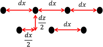
Fig. 2. Arrangement of boundary particles.
5. TEST CASE
In order to validate our model and show its capability, numerical simulations were conducted to simulate the experiments done by Lube and others (Reference Lube, Huppert, Sparks and Hallworth2004) on the collapse of a vertical, 3-D, axisymmetric column of sand. Lube and others (Reference Lube, Huppert, Sparks and Hallworth2004) pointed out that the flow behavior of granular columns relies on the aspect ratio a = H i/R i, where H i and R i are the initial height and radius of the granular column, respectively. They concluded that the final runoff distance and collapsed column height can be expressed only in terms of aspect ratio and the initial radius, and is independent of any friction coefficient. Two experiments were selected with aspect ratios of 0.9 and 2.75, and simulated using the SPH model. The initial radius of the column was 0.1 m and the numbers of fluid particles used in these simulations were 22 590 and 69 025, with 0.005 m initial distance between particles. Values of Young's modulus, the Poisson ratio, friction angle and density were 5 MPa, 0.3, 30° and 2600 kg m−3, respectively.
Figure 3 shows a comparison between the numerical and experimental results for the collapse of the sand column with a = 0.9. The numerical results show good agreement with the experimental results in terms of the final runout distance and deposit profile. However, we have indicated differences in terms of the final top shape of the cone and its sharpness. Lube and others (Reference Lube, Huppert, Sparks and Hallworth2004) indicate that a very sharp cone at the top of the final cone remains at the initial height, but in the SPH simulation, a slight decrease in the final height is observed as shown in Figure 3c. This is probably because the number of particles is not adequate to give smooth and reliable results or because of the truncation error that resulted from the approximation of spatial derivatives. Many modifications and improvements have been proposed to the SPH method to overcome these types of errors (Amicarelli and others, Reference Amicarelli2011; Hopkins, Reference Hopkins2014), but they are not considered in this paper. Moreover, a zero dilation angle of sand is assumed for simplicity, which led to a weaker soil in the SPH model (Chen and Qiu, Reference Chen and Qiu2012). In addition, the angle of repose, after the soil collapse in the simulation, is slightly smaller than that obtained from the experimental results.

Fig. 3. Comparison between experimental and numerical results: (a) initial shape of sand column; (b) simulated final profile; (c) side view of the simulated final profile; (d) experimental final profile (Lube and others (Reference Lube, Huppert, Sparks and Hallworth2004)).
Figure 4 represents a comparison between experimental and numerical results in terms of the radius of the flow front as functions of time for the case with an aspect ratio of 0.9. Even though there are small differences between the SPH and experimental results, the model is in a good quantitative agreement with the experiment, both in the position of the radius of the flow front and the timescale for their formation. Also, the flow patterns in both experiment and simulation have a primary acceleration phase followed by a deceleration phase.

Fig. 4. Typical radial displacements as functions of time for the case with an aspect ratio equal to 0.9.
Figure 5 shows a comparison of the normalized final deposit height of the SPH simulations in the two cases, together with a fit curve from the experimental data observed by Lube and others (Reference Lube, Huppert, Sparks and Hallworth2004). It illustrates that the computed final deposit height is slightly lower than the values predicted from the experimental data.

Fig. 5. Comparison of normalized final deposit height between the simulations and experimental results.
6. RESULTS AND DISCUSSIONS
In this section, SPH is applied to simulate Geotechnical materials through three main problems to test the abilities of the proposed model. First, SPH is applied to simulate a small-scale granular avalanche flow down an inclined surface obstructed by a group of stake rows with different spacing. Through this case study, we show that SPH can capture the deposition shape at the end of the slope. Next, the SPH model is applied to simulate the 3-D granular free-surface flow around a circular cylinder which considers common obstacles such as tree trunks, and is of fundamental practical interest to the design of pylons that are able to show steadfastness in front of such kinds of flows (Sovilla and others, Reference Sovilla, Schaer, Kern and Bartelt2008).
Finally, the SPH method is used to carry out 3-D simulations of the gravity granular flow past a pyramid wedge (tetrahedral) which is used as a typical defense structure to divert flow and guide avalanches past protected buildings and other areas.
6.1. Gravity granular flows past a group of stake rows
6.1.1. Model description
A laboratory experiment was conducted by Yellin and others (Reference Yellin, Saito, Kimura, Otsuki and Shimizu2013) in the Hydraulics Research Laboratory at Hokkaido University. Figure 6 shows a schematic diagram illustrating the dimensions of the experiment and the initial position of a sand mass. The model was built from two wooden panels; each of them is 1.80 m long and 0.90 m wide. The first panel was inclined at 20° with the horizontal and the obstacles were placed at a distance of 30 cm from its top. The inclination of the second panel was 45°. An amount of quartz sand (2.04 kg) was initially filled in the starting box, located 30 cm from the top of the second panel. Grid lines were drawn on the panels, with 10 cm intervals in order to know the particle positions and their speed.

Fig. 6. Schematic sketch of the avalanche experiment.
This experiment was originally conducted as a starting point to design energy dissipators for the snow avalanche. We used three different types of obstacles, as shown in Figure 7.
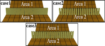
Fig. 7. The different types of obstacles, and areas name.
Case 1: 1 cm square columns with 1 cm spacing.
Case 2: 2 cm square columns with 2 cm spacing.
Case 3: 1 cm square columns in a staggered shape.
6.1.2. Numerical simulations
The simulation of the granular flow was carried out using the proposed SPH model. The number of particles used to simulate the soil mass was 12 054, with 0.005 m initial distance between particles. These particles had the following properties: density ρ = 1500 kg m−3, Young's modulus E = 150 MPa, internal friction angle ϕ = 32° and Poisson ratio υ = 0.3.
6.1.3. Results and analysis
Figures 8–10 show the comparisons between the experimental and numerical results in terms of the final deposition shape and particles spreading at the three cases. A good agreement between the simulated and experimental results is found when we use a suitable number of particles. However, we notice that the final simulated deposition shapes are almost symmetrical around the longitudinal centerline, unlike the deposition forms resulting from the experiments. Also, in Cases 1 and 3, some particles were deposited above the obstacle in the experimental results while in Case 2, with the wider spacing between obstacles, there is no deposition above the obstacle. The results are successfully confirmed by the numerical results. Figure 11 represents a comparison between the experimental and numerical results in terms of the position of the leading edge vs time for Case 1. Although there are small differences between the SPH and experimental results, the positions of the leading edge stay almost the same in both the numerical and experimental results until t = 1.4 s. After that, the speed of the particles in the experiment decreased, and finally stopped at t = 3.0 s, while the simulated particles moved faster until t = 1.7 s, then gradually stopped at t = 3.2 s.

Fig. 8. Comparison between: (a) experimental and (b) numerical results in term of the final deposition shape (Case 1).

Fig. 9. Comparison between: (a) experimental and (b) numerical results in term of the final deposition shape (Case 2).

Fig. 10. Comparison between: (a) experimental and (b) numerical results in term of the final deposition shape (Case 3).
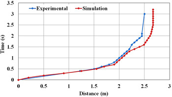
Fig. 11. Comparison in terms of position of leading edge with time (Case 1).
In order to investigate the efficiency of the obstacles, Yellin and others (Reference Yellin, Saito, Kimura, Otsuki and Shimizu2013) designated the area upstream of the obstacles as Area 1, and the area downstream Area 2, as shown in Figure 7, and then they measured the weight of deposited material (A1 and A2 respectively) in each area and derived an obstacle efficiency factor: Efficiency factor (%) = (A1 + A2)/2.04 kg × 100%. In our simulations, we counted the number of deposited particles in both the areas. Table 1 shows the efficiency factor for the experimental and simulated results. The efficiency factor from the experimental results in all cases is slightly greater than that calculated from the SPH results; the error is about 5%.
Table 1. The efficiency factor for the experimental and simulated results in the different cases

6.2. Granular free-surface flow around a circular cylinder
6.2.1. Model description
Small-scale experiments were carried out by Cui and others (Reference Cui and Gray2013) to investigate the gravity-driven free-surface flow of a granular avalanche around a circular cylinder.
The experimental device was built using a smooth Plexiglas chute that is 300 mm wide and 600 mm long and is inclined at an angle ζ = 36° to the horizontal as shown in Figure 12. Sand was loaded into a hopper at the top of the chute, and a gate was used to control the height and flux of material entering the chute. A 30 mm diameter circular metal cylinder was attached to the center of the chute 300 mm downstream from the inflow gate, so that its axis was normal to the inclined plane.

Fig. 12. Experimental setup showing the flow past a circular cylinder on a chute inclined at an angle ζ to the horizontal (Cui and others (Reference Cui and Gray2013)).
All phases of the experiments were totally registered with a video and photo camera. Pictures were taken at a rate of 25 s−1 in order to show how the bow shock and the granular vacuum are formed in a close-up region near the cylinder.
6.2.2. Numerical simulations
In total, 234 675 soil particles with an initial mean separation of 0.002 m were used to simulate a sand mass. They were placed in the hopper at the top of the chute. Table 2 shows the values of the parameters used to simulate the flow of a granular avalanche around a circular cylinder.
Table 2. The values of the soil parameters used to simulate the flow of granular avalanche around a circular cylinder
The gate opening height is 0.4 dimensionless units, where the cylinder diameter D = 30 mm is used in dimension scaling (30 mm = 1 dimensionless unit). On the other hand, the velocities are scaled by $\sqrt {Lg} = 0.54{\rm } {\rm m s}^{ - 1} $
and time is scaled by
$\sqrt {Lg} = 0.54{\rm } {\rm m s}^{ - 1} $
and time is scaled by $\sqrt {L/g} = 0.055\,{\rm s}$
.
$\sqrt {L/g} = 0.055\,{\rm s}$
.
6.2.3. Results and analysis
Figure 13 presents a series of snapshots of the avalanche hitting the circular cylinder, showing the particles positions and free-surface shape together with the velocity field at different times. The result obtained by the SPH method is compared with the experimental images and the superimposed computed boundary obtained from the hydraulic avalanche model solution by Cui and others (Reference Cui and Gray2013). The time intervals between snapshots are equal to 0.72 non-dimensional units. Since the gate was not in the camera shots, the comparison of the simulation and the experiment starts from the distance x = 8 units at time t = 7.4 units.

Fig. 13. Comparison between computation and experiment results at different time steps (t = 7.4, 8.12, 9.56, 10.28 and 12.44 dimensionless units) showing the continuation of the time-dependent development of a bow shock and a vacuum boundary.
When the particles are released from the gate, the flow front starts to propagate uniformly, and the flow was fast and thin. When the particles start to hit the cylinder, the flow continues to propagate downstream except for those particles that collide with the obstacle and are largely affected by the obstacle (Figs 13b and f). A jump in the flow thickness and velocity, which is named as ‘bow shock wave’ starts to develop at the front of the cylinder by t = 8.84 units (Figs 13c and g). The bow shock continues to grow slightly in height and to move upstream until the oblique shocks on either side of the obstacle are almost fully developed by t = 10.28 (Figs 13d and h). By t = 12.44 units, (Figs 13e and i), the flow reaches a steady-state regime with no further growth within the field of view, and the granular vacuum clearly appears downstream of the cylinder and forms a triangular shape.
The developing process of the bow shocks by the present computation is in a close agreement with the experimental results. For the vacuum boundary, the closed triangular region obtained by the simulation seemed to be larger than the one formed in the experiment. Generally, we can conclude that this model captures most of the essential aspects of the observed phenomena.
6.3. Gravity granular flows past tetrahedral wedge
6.3.1. The model description
The tetrahedral wedge was proposed to protect the Schneefernerhaus at Zugspitze, Germany, against a large avalanche with a 100 a recurrence equal to a snow layer of 8 m depth moving down the mountain (Tai and others, Reference Tai, Wang, Gray and Hutter1999). The Schneefernerhaus was an old hotel, which was renovated and transformed into a research laboratory for environmental and climatological research in 1999. It is situated on a mountain slope inclined by ~45° (Fig. 14a).

Fig. 14. (a) The Schneefernerhaus at the Zugspitze, Germany at 2700 m on a rather planar mountain slope inclined at ~45°. (b) A model reproduction together with tetrahedral wedge type avalanche protection.
In a first study aimed at protecting this building against avalanche, a tetrahedral wedge was designed to divert the flow and guide the snow pass the building on either side. Tai and others (Reference Tai, Noelle, Gray and Hutter2002) decided to carry out laboratory experiments to simulate this event. Two models at scales 1 : 100 and 1 : 300 were used to perform their experiments. In our study, the two-scale experiments were simulated using the current SPH model. In the experiments, the mountain flank modeled as an inclined plane of a 45° slope angle is made from Plexiglas. The models of Schneefernerhaus and of the wedge were cut from plastic and wood blocks, respectively.
Semolina flour grains, 0.8 mm in diameter, and plastic beads were used as the model of ‘dry snow’. The internal angle of friction of these materials was within the range of the snow. The used materials were initially filled in a tank with a gate at the upstream end of the slope. Figure 14b shows the experimental setup with scale 1 : 300.
6.3.2. Numerical simulations
The number of particles used to simulate the semolina and plastic beads masses was 165, 000, with 0.002 m initial distance between particles. The material constants used in the calculation for the two cases are illustrated in Table 3.
Table 3. The material parameters used to simulate the gravity granular flows past tetrahedral wedge

6.3.3. Results and analysis
Figure 15 shows three snapshots of the motion of a layer of semolina. This layer represents the motion of an 8 m layer down the slope, past and around the obstacle and the Schneefernerhaus building at three different stages compared with numerical results of the SPH simulations.

Fig. 15. Caparison between experimental and numerical results at three different stages showing the motion of a layer of semolina past and around the obstacle and the Schneefernerhaus building.
From the snapshots, we can see how the obstacle diverts the flow. A normal shock is formed at the pyramid top and extends on both flanks of the pyramid to form an oblique shock, which can be clearly seen from the streamlines in the photograph as well as the particles spreading in the numerical simulation. At the downstream region of the obstacle, the flow rapidly spreads in the transverse direction and forms an expansion fan far from the protected area, which is also well described by the SPH simulation.
Figure 16 shows a comparison of three different results. An experimental photograph (scale 1 : 100), the numerical results obtained by applying the Savage and Hutter (Reference Savage and Hutter1989) theory using the two-dimensional (2-D) NOC scheme (Jiang and Tadmor, Reference Jiang and Tadmor1997), and the SPH simulation, representing the steady flow past the defense structure. The oblique shocks on both sides of the defense structure are seen from the streamlines in the experiment, computed flow thickness from the 2-D NOC scheme, and the particle distribution together with the velocity field. Also, the particle-free region was formed, which shows that the protected zone is well described in the SPH results.

Fig. 16. Comparison between: (a) the experimental results (scale 1 : 100), (b) numerical results obtained from the 2-D NOC scheme and (c) SPH simulation representing the steady flow past the defense structure.
From the above results, it is clear that the SPH method can well describe the properties of the flow around the tetrahedral obstacle and can quantitatively describe the protection region.
Figure 17 demonstrates a horizontal cross section of the flow depth along the line x = 5.6 dimensionless units, which crosses the upper part of the pyramid at t = 10 dimensionless units. The solid curve represents the Savage and Hutter (Reference Savage and Hutter1989) theory solution utilizing the 2-D NOC scheme, and the particles distribution gives the cross-sectional shape obtained by the SPH simulation.
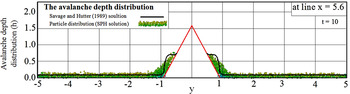
Fig. 17. Cross section of the avalanche depth distribution along the line x = 5.6 through the top of the pyramid.
The shocks are visible on either side of the defense structure. Behind the shock, the avalanche thickness is approximately four times that of the Savage and Hutter theory solution, and three times that of the present SPH model as large as in front of the shock. In the two solutions, the shocks are symmetrical though they have different shapes.
7. CONCLUSION
A novel 3-D computational model based on the SPH method has been developed for simulating the granular flow past different types of obstacles. The elastic–perfectly plastic model has been implemented in the SPH framework to model the granular materials. The present model was validated by an experiment on the collapse of the 3-D axisymmetric column of sand. Good agreement was observed between the numerical and experimental results.
Granular flow past three types of obstacles, a group of stake rows with different spacing, circular cylinders and tetrahedral wedge have been numerically simulated using the present SPH model. The computational results were compared with the experimental results and two existing numerical results to check the capabilities of the proposed model. The numerical results in the first case in terms of the final granular deposition shapes, spreading of the particles and the position of the leading edge are found to be in good agreements with the experimental results. Although the efficiency factor from the experimental results in all cases is slightly greater than the calculated values from the SPH results, the error is ~5%.
The simulation of granular free-surface flow around a circular cylinder, and a tetrahedral obstacle shows that the SPH method can capture and describe the formation of the bow shock, normal shock and oblique shock around the obstacle, and can describe the protected area as observed in the experiments, the hydraulic avalanche model solution and Savage and Hutter (Reference Savage and Hutter1989) theory solution.
This study suggests that SPH could be a powerful method for solving problems dealing with granular materials subjected to large deformation and could be used to design real avalanche defenses.
ACKNOWLEDGEMENT
A. M. Abdelrazek would like to acknowledge the financial support from the Japanese government (MEXT), and JSPS KAKENHI Grant Number 15F15369.


 Open access