


1. INTRODUCTION
Over the last 50 years, the Greenland and Antarctic ice sheets have been extensively surveyed using radio echo sounding (radar), allowing researchers to determine ice thickness and internal stratigraphy of these large ice bodies (e.g. Evans and Smith, Reference Evans and Smith1969; Harrison, Reference Harrison1973; Robin and others, Reference Robin, Drewry and Meldrum1977; Drewry and Meldrum, Reference Drewry and Meldrum1978; Dahl-Jensen and others, Reference Dahl-Jensen1997; Lythe and others, Reference Lythe and Vaughan2001; Paden and others, Reference Paden, Akins, Dunson, Allen and Gogineni2010; Bamber and others, Reference Bamber2013; Keisling and others, Reference Keisling2014; MacGregor and others, Reference MacGregor2015) and revealing insights into their past and present flow dynamics (e.g. King and others, Reference King, Hindmarsh and Stokes2009; Sime and others, Reference Sime, Karlsson, Paden and Prasad Gogineni2014; Bingham and others, Reference Bingham2015; MacGregor and others, Reference MacGregor2015; Winter and others, Reference Winter2015; Cavitte and others, Reference Cavitte2016; Christianson and others, Reference Christianson2016). While the majority of glaciological radar studies were conducted using airborne surveys or ground-based traverses, stationary phase-sensitive radio echo sounders (pRES) have recently emerged as an important tool to measure one-dimensional (I-D) vertical strain on ice sheets (Kingslake and others, Reference Kingslake2014; Nicholls and others, Reference Nicholls2015; Kingslake and others, Reference Kingslake, Martín, Arthern, Corr and King2016) and basal melting on ice shelves (Corr and others, Reference Corr, Jenkins, Nicholls and Doake2002; Jenkins and others, Reference Jenkins, Corr, Nicholls, Stewart and Doake2006; Dutrieux and others, Reference Dutrieux2014; Marsh and others, Reference Marsh, Fricker, Siegfried and Christianson2016) with both high accuracy and precision.
Nicholls and others (Reference Nicholls2015) and Lok and others (Reference Lok, Brennan, Ash and Nicholls2015) briefly described the potential of pRES to be deployed in an imaging mode using a multiple-input multiple-output (MIMO) array system, which has the capability to sequentially switch between up to eight transmitting (Tx) and receiving (Rx) antennas (yielding up to 64 virtual antenna pairs) with the aim to image the basal topography of ice sheets. Similar to phased arrays, a MIMO system involves the transmission and reception of its signals (and combinations thereof) from multiple transmitting and receiving antennas, arranged in such a way to create a gridded synthetic aperture from the midpoints of each virtual antenna pair. The combined signals from the antennas are then manipulated to electronically steer the array's radiation pattern in desired directions. Although the use of phased and MIMO arrays for through-air imaging are developing traction due to their wide virtual aperture and high accuracy in detecting and tracking moving targets (e.g. Li and others, Reference Li, Stoica and Zheng2008), its application to subsurface imaging through ice is rare. While previous studies have implemented synthetic aperture experiments to image englacial and subglacial waterways and geometries by manually moving the antenna across gridded points on the glacier surface (Walford and Harper, Reference Walford and Harper1981; Kennett, Reference Kennett1989; Walford and Kennett, Reference Walford and Kennett1989), only recently have radars been able to successfully and instantaneously image the full 3-D subglacial topography using multiple antennas (Paden and others, Reference Paden, Akins, Dunson, Allen and Gogineni2010; Jezek and others, Reference Jezek2011; Wu and others, Reference Wu2011).
Here, we use a MIMO pRES array with 16 real antennas on Store Glacier in West Greenland to explore its imaging capabilities. We investigate the geometry of internal layers and the glacier bed obtained from three field sites. Additionally, by investigating the effects of antenna array parameters that control the radiation patterns, we demonstrate the importance of the array configuration on the resulting imagery. Finally, we highlight key array parameters to be considered in future pRES system deployments.
2. METHODS
2.1. Location and study area
Store Glacier (Qarassap Sermia) is a fast-flowing, marine-terminating glacier in the Uummannaq region in western Greenland (Qaasiutsup Kommunia; Fig. 1a). The glacier has a catchment of 35 000 km2 and is 5 km wide at the terminus, where the glacier flows at ~6300 m a−1 (Rignot and Mouginot, Reference Rignot and Mouginot2012; Morlighem and others, Reference Morlighem2016). While many surrounding glaciers have recently experienced dynamic thinning due to acceleration and retreat of their termini, Store Glacier has exhibited little change in both mass balance and overall terminus position since 1968, exhibiting only a 200 m seasonal oscillation in the terminus position (Weidick, Reference Weidick1995; Howat and others, Reference Howat, Box, Ahn, Herrington and McFadden2010; Box and Decker, Reference Box and Decker2011). This stability is due to topographic narrowing and grounding near the glacier's terminus (Todd and Christoffersen, Reference Todd and Christoffersen2014; Morlighem and others, Reference Morlighem2016). However, with a 1000 m-deep trough extending 30 km inland from the margin, Store Glacier may experience rapid and prolonged retreat if the terminus stability is undermined by warming ocean temperatures (Morlighem and others, Reference Morlighem2016).
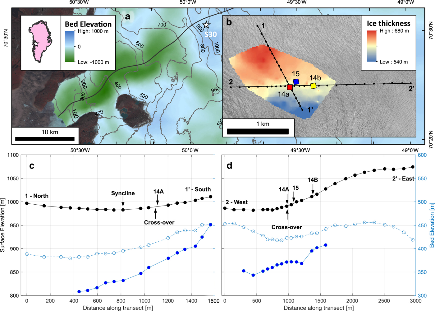
Fig. 1. (a) Map of Store Glacier and location of study area (S30), with bed elevation (Morlighem and others, Reference Morlighem2017) overlain with surface elevation contours (GIMP DEM; Howat and others, Reference Howat, Negrete and Smith2014) and central flowline (thick black; Todd and Christoffersen, Reference Todd and Christoffersen2014). (b) Study area (S30) showing the location and orientation of the three radar arrays and the local ice thickness, interpolated from quasi-monostatic (1Tx/1Rx) pRES measurements. Map is superimposed on a WorldView-2 image at 2 m resolution (27 July 2008). (c) Surface (black) and bed (solid blue) elevation profiles obtained by subtracting the pRES-measured ice thickness from GPS-measured surface elevation measurements (Hofstede and others, Reference Hofstede2018). The bed elevation obtained through mass conservation (dashed blue; Morlighem and others, Reference Morlighem2017) is provided for comparison. The transect (1 to 1′) is from north to south. (d) Same as (c) but for the transect (2 to 2′) running from west to east.
Our study area, S30, is within 1 km of the central flowline, ~30 km inland of Store Glacier's calving front (Fig. 1a), with an ice thickness between 600 and 650 m (70° 31′N, 49° 56′W; Fig. 1b). Here, the glacier exhibits a moderate seasonal change in ice velocities, increasing from ~600 m a−1 in winter and spring to ~700 m a−1 when the surface meltwater accesses the subglacial environment (Doyle and others, Reference Doyle2018). In general, the local ice thickness increases across-flow towards the north (Fig. 1b) and drapes consistently with the bed downstream (Fig. 1d), while to the south, the flow is constrained by increasing bed elevation (Fig. 1c). Though vertically offset by 0–100 m at several locations (e.g. at the 400 m marker in Fig. 1d), the bed elevation profiles obtained from pRES bed soundings show similar trends of topographic change compared with other catchment-wide interpolations of bed topography, for example, calculated from mass conservation (Fig. 1c,d; Morlighem and others, Reference Morlighem2017).
2.2. Radar and antenna array architecture
Over three-field campaigns (Table 1), three identical pRES instruments were deployed in an 8 × 8 MIMO array arrangement within S30 (Fig. 1b). The pRES instrument operates over the frequency range 200–400 MHz and is centred at 300 MHz, which allows for sufficient ice penetration while its phase sensitivity allows it to achieve millimetre-depth precision. The design and technical details for the instrument's radar board are described in detail in Brennan and others (Reference Brennan, Lok, Nicholls and Corr2014) and the practical aspects and limitations of its deployment in a quasi-monostatic (1 Tx/1 Rx) configuration are presented in Nicholls and others (Reference Nicholls2015).
Table 1. Timing and orientation of radar arrays as shown in Fig. 1b
a Relative to the principal flow direction (262°; W of SW).
The MIMO array used in the field experiments consisted of two rows of antennas on the ice surface oriented orthogonal to each other (Fig. 2a) and mounted on a wooden frame to stabilise the arrangement against differential ablation on the ice-sheet surface (Fig. 2c). Each row comprised eight cavity-backed bowtie antennas functioning in either transmit (Tx) or receive (Rx) mode, therefore synthesising a planar grid of 64 virtual antenna pairs (Lok and others, Reference Lok, Brennan, Ash and Nicholls2015), each recording one chirp for a burst total of 64 chirps (~1 min duration). All bowtie antennas were constructed in-house for a centre frequency f c = 300 MHz with a bandwidth of 200 MHz. The dimensions of the antenna used in this study were tuned to operate on the ice surface and each was housed in a square corrugated plastic box of dimensions 820 mm × 820 mm × 300 mm (Fig. 2). Each row of antennas were arranged end-to-end, thus giving a virtual antenna pair separation of δ = 410 mm (equivalent to 0.74 × λ c, the central wavelength, assuming a dielectric constant of ice of εr = 3.18).
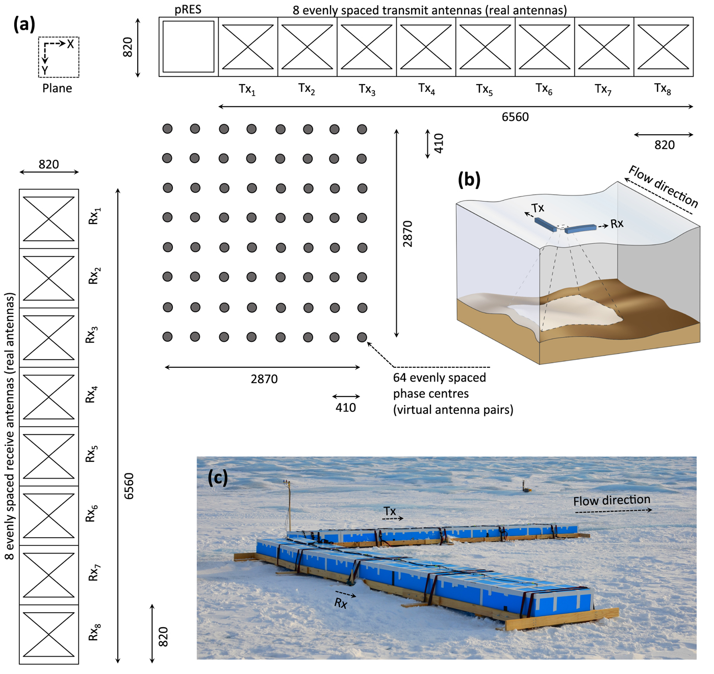
Fig. 2. (a) Schematic diagram (along the X–Y plane, where the Z-axis points into the diagram) showing the field configuration of the planar MIMO antenna array, composed of 8 transmitting (Tx) and 8 receiving (Rx) bowtie antennas oriented in two orthogonal linear arrays, producing 64 virtual antenna pairs. (b) Conceptual diagram showing the footprint of the deployed antenna array. (c) Photo of field setup of the MIMO antenna array at site 14a (70° 31′ 02″ N, 49° 55′ 50″ W as of 7 May 2014; Fig. 1), with the principal direction of flow: oriented west-southwest (262°). All measurements shown are in mm.
2.3. Digital signal processing
In addition to the processing steps described in Brennan and others (Reference Brennan, Lok, Nicholls and Corr2014), we processed each of the 64 virtual antenna pairs using exact geometrical correction based on path lengths Eqn (1). This method is a direct and convenient way of processing the image in horizontal depth layers and sequentially building a 2- to 3-D depth image. Here, the beam is digitally steered by manipulating the received phase signals of each virtual antenna pair from a desired angle of incidence through combinations of constructive and destructive interference. Through this technique, the overall antenna array can scan rapidly through both the along- and cross-range of the incident ice column.
Denoting the range profile of the (x m, y n) pixel by E(x m, y n, r), the (X, Y) pixel amplitude at a specified depth beneath the ice surface R is:
 $$\eqalign{ P\left( {X,Y} \right) & = \sum\limits_{m = 1}^M {\sum\limits_{n = 1}^N E } \left( {x_m,y_n,d\left( {X,Y,x_m,y_n} \right)} \right) \cr & \ \ \ \, \exp \left[ { - j\displaystyle{{4\pi d\left( {X,Y,x_m,y_n} \right)} \over {\lambda _{\rm c}}}} \right]} $$
where λ c is the wavelength corresponding to the pRES chirp's centre frequency and where d is the trigonometric distance from (x m, y n) to (X, Y):
 $$d\left( X,Y,x_m,y_n \right) = \sqrt{ \left(X-x_m\right)^2 + \left(Y-y_n \right)^2 + R^2 }$$
so that when the angle of incidence is 0, d = R.
The exponent in Eqn (1) encompasses the phase of the up-chirp:
 $$\phi = \displaystyle{{ + 4\pi d} \over {\lambda _{\rm c}}}$$
and so the compensation is the negative of this term.
For the experiments presented herein, we use M = N = 100 and a depth range of 10–650 m with a depth step of 1 m.
2.4. 2-D and 3-D vertical section processing
Using the resulting 3-D images, we extracted 2-D horizontal and vertical cross-sections for analysis (Fig. 3). Horizontal sections are aligned parallel (i.e. along the X–Y plane) and vertical sections are aligned orthogonal to the pRES synthetic aperture (i.e. along the X–Z and the Y–Z plane; Fig. 3). To minimise the effect of instrumental and environmental noise, all horizontal and vertical sections were subjected to first a 2-D median filter consisting of a 4 × 4 matrix moved over the image, and then a 2-D peak convolution using a Gaussian low-pass filter with the same moving matrix dimensions. While the post-filtering location and shape of internal layers did not significantly change when varying the window size, filtering reduced the amount of erroneous internal layers (identified through an automated peak-detection function) by ~85%.
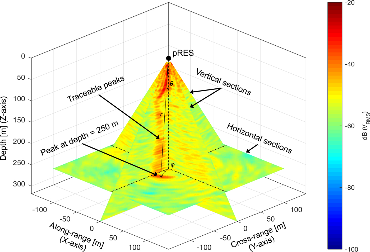
Fig. 3. Nomenclature of 2-D cross-sections. Within each vertical section, peaks in returned backscatter power are identified and can be traced with increasing depth. At specific depths, the location of these peaks was used to triangulate the peak within the corresponding horizontal section.
With the exception of the deployment at site 14a, which was aligned to true north resulting in a slight offset of 12° relative to the principal flow direction (262°), all arrays were oriented relative to flow (Table 1). Therefore, while the vertical images obtained beneath sites 14b and 15 depict the ice column oriented parallel and perpendicular to flow, the image obtained beneath site 14a, respectively depict the ice column oriented north to south and east to west.
Within each vertical section, we identified the spherical location of peaks (r, θ, φ) with a returned backscatter power above −50 dB V RMS. Doing so revealed a series of peaks traceable through increasing depth (Fig. 3). Although the radial distance of the peak to the antenna array (r) and the angle from nadir (θ) can be accurately determined within each vertical section, the azimuth (φ) is not yet constrained due to the pre-set orientation of the vertical sections (φ = 0, 90, 180, or 270°; Fig. 3). Therefore, using the traced peaks within each vertical section as a guide, we then located the identified peaks in 3-D through sequential horizontal sections, resolving the third spherical coordinate φ (Fig. 3).
Range migration begins to have a significant effect when the number of linearly-spaced elements is at least 1 + 4/B f, which is 7 for the parameters of the pRES system given B f = 2/3 (a fractional bandwidth of 200/300 MHz; Brennan and others, Reference Brennan, Rahman and Lok2015). The configuration of the 8 × 8 planar MIMO antenna array (Fig. 2a) exceeds this limit very slightly, and therefore the effect of range migration is minimal and only marginally affects the outer limits of the scan angle range. Therefore for simplicity, we do not apply range migration correction.
3. IDENTIFICATION AND INTERPRETATION OF INTERNAL LAYERS
3.1. Vertical stratigraphy of the ice column
All pRES vertical sections acquired on Store Glacier show similar internal stratigraphy through depth, with the sections divided into four distinct bands (Fig. 5). Through the majority of the vertical sections, a series of peaks, which we interpret to be dominant internal layers, can be traced from the ice surface (black dots, Fig. 5). The traced peaks all curve away from nadir with depth, and extend to considerable (~300 m) depths, particularly those aligned perpendicular to flow (i.e. along the Y–Z plane). Besides the identified peaks, there exists some clustering in reflections away from the traced peak trajectory, particularly between 300 and 500 m depth.
The upper 30–80 m of the vertical section is dominated by closely-spaced high (− 40−20 dB V RMS) signal strength reflections. We do not attribute the source of the observed near-surface clutter without further field investigations; however, these near-surface inhomogeneities could be due to any or a combination of (i) Fresnel diffraction within the near-field region (Yamaguchi and others, Reference Yamaguchi, Mitsumoto, Kawakami, Sengoku and Abe1992); (ii) englacial heterogeneities (e.g. water-filled pockets, cracks, veins, conduits) within the upper glacier surface (Smith and Evans, Reference Smith and Evans1972; Watts and England, Reference Watts and England1976; Kanagaratnam and others, Reference Kanagaratnam, Gogineni, Ramasami and Braaten2004); and (iii) presence of surface crevasses (Rignot and others, Reference Rignot, Mouginot, Larsen, Gim and Kirchner2013; Colgan and others, Reference Colgan2016), of which the latter two are abundantly present at S30 (Hofstede and others, Reference Hofstede2018).
Beyond depths of 500 m, the returned signal strength drops markedly, indicating a ~100 m thick transparent region of ice above the ice/bed interface. This region in our study is located close to an observed change in crystal fabric orientation transitioning to anisotropic Wisconsin-aged ice detected from seismic experiments (Hofstede and others, Reference Hofstede2018) and the onset of high deformation inferred from borehole-installed tilt sensors both conducted within S30 (Doyle and others, Reference Doyle2018). While the enhanced shearing observed at S30 may further deteriorate the presence of layers within this region, we are still able to detect some deep reflectors (e.g. at 580 m at site 14b), implying that the reduction in signal strength is caused by an attenuation in the power of the received signal. Further investigations are needed to provide definitive conclusions as to whether the lack of internal layers depth range represents these changes in ice properties.
The ice/bed interface, located between 600 and 640 m depth, is consistently identified in all sections as an abrupt increase in signal strength (+60 dB V RMS). The signal strength is sustained beyond this range to at least 650 m, which is the lower boundary applied to our images. For reasons discussed below, we discount the curved bed geometry seen in all sections as an artefact of processing, and instead focus on the traceable peaks and their representation as internal layers.
3.2. Simulation of the vertical section
Although at first glance the traced peaks identified in all vertical sections within S30 (Fig. 5) may visually resemble surface crevasses or large moulins (e.g. Arcone and Delaney, Reference Arcone and Delaney2000), the minimum depths to which all the traced peaks at least propagate to (>100 m), are all of order of magnitude beyond field observations of crevasses and likely would not penetrate deeper than ~30 m without the presence of meltwater due creep closure from the stress supplied by the surrounding ice (Colgan and others, Reference Colgan2016). Therefore, to determine the cause of these traced peaks, we conducted a series of simulations that reconstructs a synthetic 2-D glacier vertical section varying the parameters of the array factor of the antenna array deployed in the field (Fig. 4; see Appendix). The array factor (F a) characterises how the power of a radar-transmitted signal is spatially distributed (i.e. the height and width of the main lobe and sidelobes, and the presence of grating lobes) across the swath of scanning angles (θ) and combined with the radiation pattern of a single virtual antenna pair (element factor; F e) produces the transmitted and received signal of the overall antenna array (F):
 $$F\left(\theta\right) = F_{{\rm e}}\left(\theta\right) F_{{\rm a}}\left(\theta\right) = F_{{\rm e}}\left(\theta\right) \sum_{k=1}^{K} \exp\left[ -j \left(K-k\right) k_0 \delta \sin\left(\theta\right)\right]$$
for a linear system of K virtual antenna pairs uniformly spaced δ m apart (Huang and others, Reference Huang2011), where k 0 = 2π/λ c is the free space wave number. The antenna array's performance can be optimised by manipulating Eqn (4)'s key parameters, namely (i) the element factor (F e); (ii) the number of linear virtual antenna pairs (K); and (iii) the separation between virtual antenna pairs (δ). Accordingly, the series of simulations (Fig. S1-3 in Supporting Information) varied these three parameters.
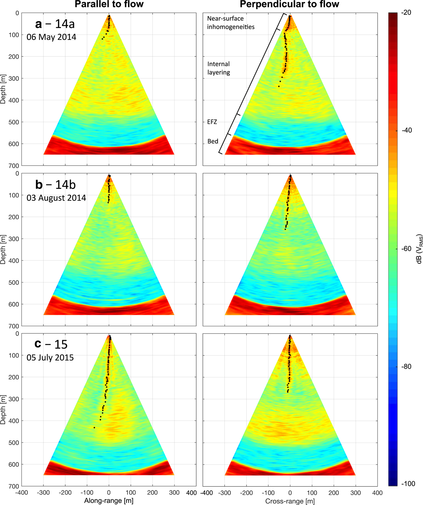
Fig. 4. 2-D vertical sections within S30 acquired along (left column) and across (right column) the ice flow direction (262°). Black dots show identified peaks in returned backscatter power (>−50 dB VRMS) traceable through depth, and vertical bands indicating types of layering are shown in (a). Sections were acquired at (a) site 14a on 6 May 2014 (offset by +12°; Table 1); (b) site 14b on 3 August 2014; and (c) site 15 on 5 July 2014. Fig. 1b and Table 1 shows the location and orientation of each deployment within S30.
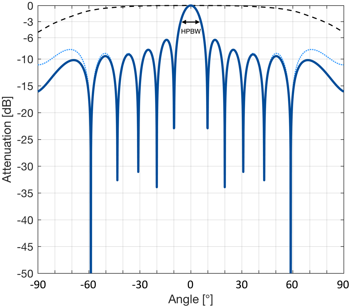
Fig. 5. Radiation patterns of the overall array (F; solid blue), the element factor (F e; dashed black) and the array factor (F a; dotted blue) using the setup as described in Fig. 2a. The half-power beamwidth (HPBW) of both F and F a, indicated by arrows, is ±6°.
Specifically, the simulations track the transmission and reflection of a signal beam (Eqn 4) across a range of angles through depth, and reconstructs a vertical glacier along-flow section by vertically stacking the received signals through depth, as described in the Appendix. The signal beam was generated from an 8-antenna linear array using the array factor derived from the field configuration (Fig. 2a). The synthetic glacier vertical section (synthetic section) used as input to all simulations (Fig. 6a) included several artificial features typical of radargrams of ice sheets, notably four internal layers at various slope angles and a flat, subglacial layer with an undulating bed and a small topographic protuberance 20 m high, 50 m wide, with its apex located 100 m left of nadir (equivalent to −9.46°; Appendix).
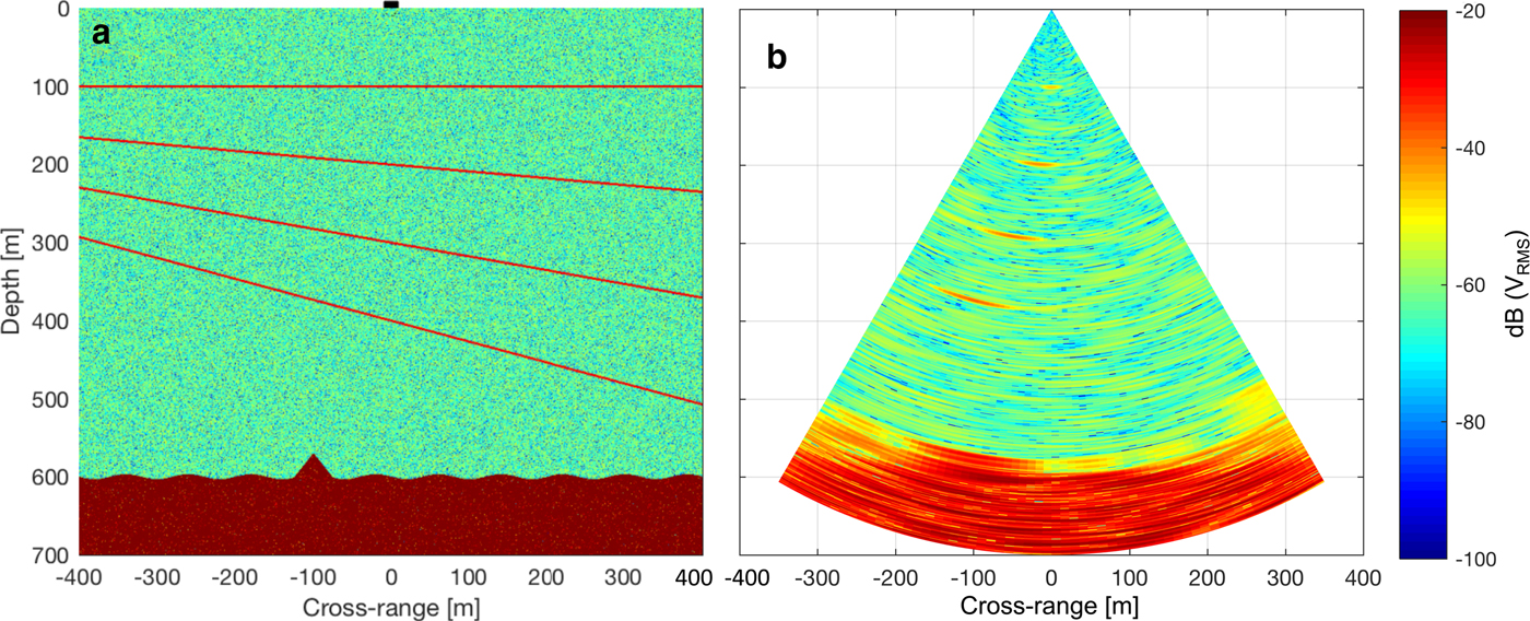
Fig. 6. (a) Synthetic glacier vertical section as input to model simulations. The location of the array is at (0, 0), indicated by a black square. (b) Corresponding reconstructed glacier vertical section parameterised using the setup as described in Fig. 2a.
By assuming internal layers to be specular reflectors (Drews et al. Reference Drews2009, Holschuh et al. Reference Holschuh, Christianson and Anandakrishnan2014, Cavitte et al. Reference Cavitte2016; Appendix), the transmitted signal is only reflected from the internal layer when the incident ray beam path is at or close to normal relative to the layer plane (Fig. 7). The incorporation of this assumption into the simulation importantly reconstructs the synthesised internal layers (Fig. 6a) into a peak of concentrated returned backscatter visually similar to field-acquired sections at S30 (Fig. 5). Geometrically, the centre of the simulated peak, where returned backscatter power is highest, is normal to the slope of the synthesised internal layer, and the depth of the peak corresponds to the respective layer's mean depth (Fig. 6b). It then follows that the slope of the synthesised internal layers corresponds to the peak's angle from nadir (Fig. 7).
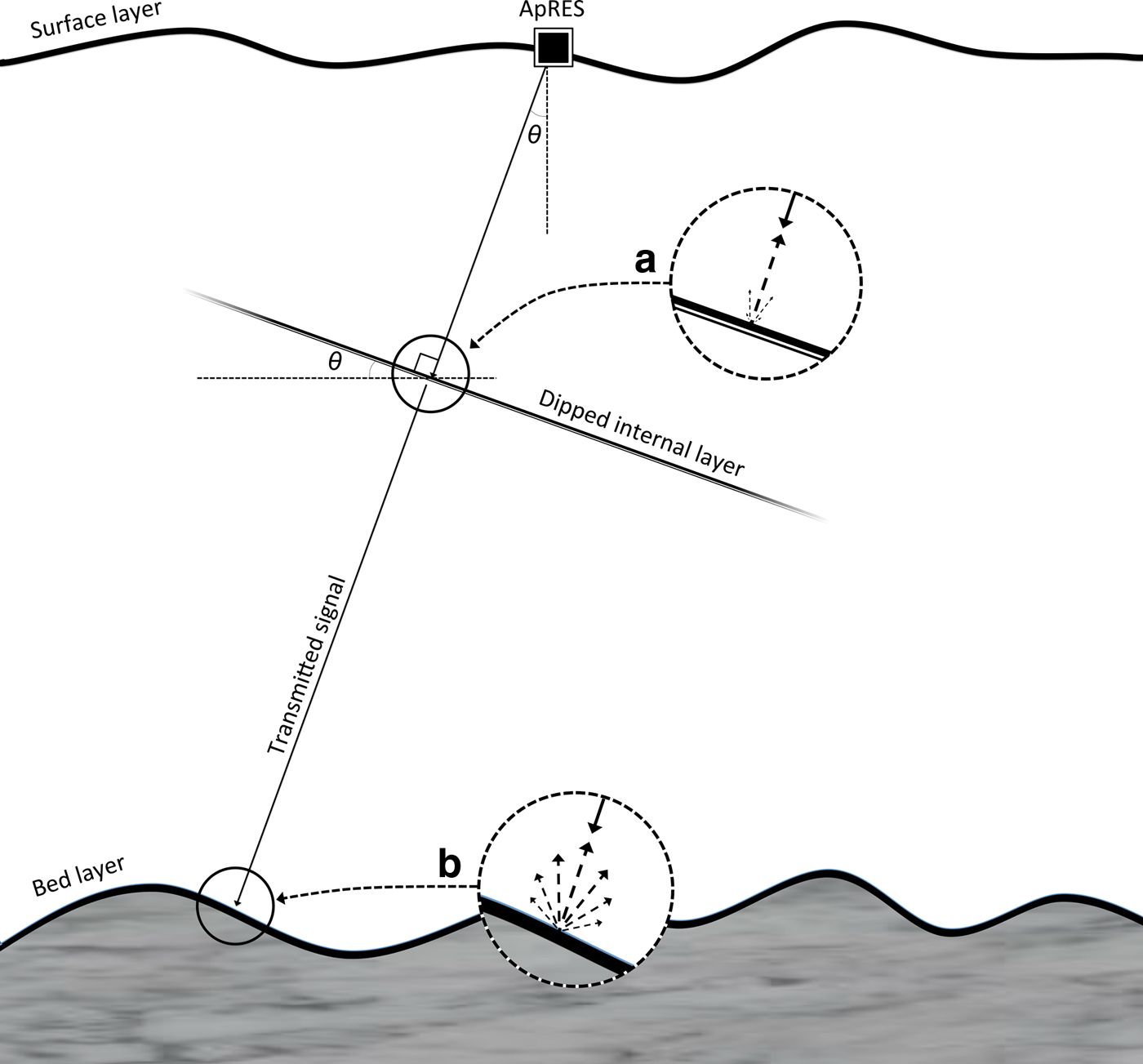
Fig. 7. Model for the scattering properties of (a) a dipped internal layer, which assumes a specular reflecting interface; and (b) a basal interface, which assumes a more diffuse interface. Further information is given in the Appendix.
3.3. Interpretation of internal layer slopes
Based on the results from the simulations, we plot the peaks identified as internal layers in Fig. 5 in 3-D to better illustrate the dipping layer (Fig. 8). Most layers within all three-radargrams slope from South to North, and the azimuth and direction of these layers agree closely with the basal topography (Fig. 1). This agreement is predominantly the case in the cross-flow direction, where the bed elevation rises to the south (Fig. 1c), but also to a lesser extent along-flow where the glacier is flowing downhill (Fig. 1d). The magnitude of the slopes observed was small overall (~2°–6°) and generally constant in tilt through depth, with the exception of more steeply-dipping layers at ~100 m depth with slopes as high as 15° beneath site 14a (Fig. 8). Although it is unlikely that moulins, water pockets, or other point scattering sources would have caused these dipping layers, as their scattering functions (spread in the 2-D image) will be wider than a specular layer, larger features such as cross-cutting crevasses or refrozen englacial water can potentially reflect anomalously high slopes if they are wide enough (a significant fraction of a Fresnel zone).
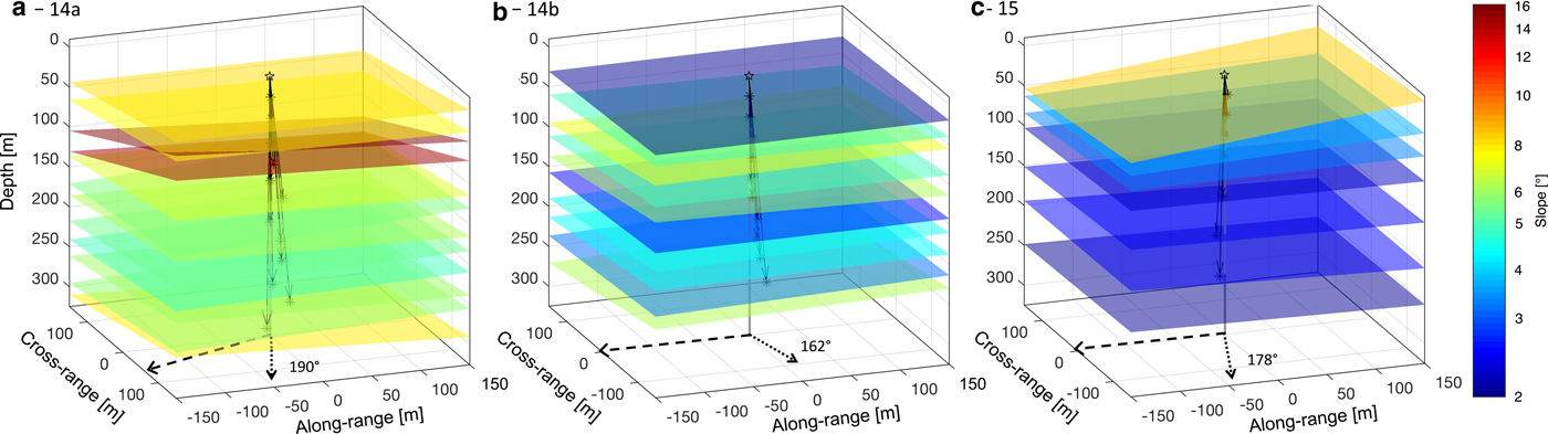
Fig. 8. 3-D planes representing the orientation and slope of identified internal layers (>−50 dB VRMS) within S30 on Store Glacier. The internal layering profiles were derived from data acquired at sites (a) 14a on 6 May 2014; (b) 14b on 3 August 2014; and (c) 15 on 5 July 2015. The orientation of the three radar arrays is shown in Fig. 1b. The principal vector normal to the dipped layers (dotted arrow) are shown relative to true north (0°), and the principal direction of flow (dashed arrow) is oriented west of southwest (262°). The magnitude of the latter two vectors are on the X–Y plane and not true to scale.
The stratigraphy of internal layers is considered representative of past and present variations in ice flow. Regions of stable and/or slow flow often develop reflector slopes that monotonically change with depth, while spatial variations in ice flow disrupt regular internal layering (Ng and Conway, Reference Ng and Conway2004; Holschuh and others, Reference Holschuh, Parizek, Alley and Anandakrishnan2017). These variations mostly result from changes to the local strain field as the ice transitions between slow and fast flow regimes; alternatively, the strain field can also be disrupted by changes to the roughness of the underlying subglacial topography (Hubbard and others, Reference Hubbard, Siegert and McCarroll2000; Siegert and others, Reference Siegert, Payne and Joughin2003; Hindmarsh and others, Reference Hindmarsh, Leysinger Vieli, Raymond and Gudmundsson2006; Bingham and others, Reference Bingham2015). Indeed, prior seismic analysis of S30 conducted by Hofstede and others (Reference Hofstede2018) revealed variations in the internal layering and the nature of the ice/bed interface within the study area, including a steep symmetric syncline located ~400 m north of array 14a (Fig. 1c) that matches the primary orientation of the identified sloping internal layers (Fig. 8). The syncline is thought to have formed in response to a combination of converging flow and basal melting. This observation, together with small-scale variations in subglacial properties, suggest that the presence of patches of different basal slipperiness is associated with variable amounts of water at the ice/bed interface. While quantitative analysis of internal layering typically requires numerical modelling of ice flow, given our knowledge of S30's subglacial environment, we believe that the spatial variability of observed englacial layer slopes through depth (Fig. 8) could be attributed to the patchy nature of the underlying bed that results in local stress variations dynamically deforming the overlying ice (Ryser and others, Reference Ryser2014). Such variations area is able to induce anomalously steep layer slopes in the middle of the ice column, allowing slopes to deviate from expected monotonic trends (Holschuh and others, Reference Holschuh, Parizek, Alley and Anandakrishnan2017). Further analysis of the subglacial conditions at the local study site, together with additional imaging pRES deployments, are needed to conclusively explain the contrasts in slope gradients, especially within the upper 100 m between the three sites at S30.
Studies of englacial layers, and their significance within the context of past and present ice flow dynamics, have so far only been based on 2-D profiling, with the third dimension, if present, projected through interpolation (e.g. Bingham and others, Reference Bingham2015; Winter and others, Reference Winter2015). Such studies usually require ground- or air-based radar traverses that typically demand extensive logistical support. The advent of an instrument to measure the 3-D variability of internal layers with depth represents an additional method to investigate the ice flow structure over a large spatial area. In particular, the use of multiple imaging pRES arrays may complement traditional surveys in identifying potential ice-coring and/or subglacial access hot-water drilling sites, both of which require prior knowledge of the internal layer geometry to understand the local ice flow regime.
Past studies using pRES have tracked the vertical movement of internal layers through time, and have used this information to extract basal melt rates beneath Antarctic ice shelves (Corr and others, Reference Corr, Jenkins, Nicholls and Doake2002; Jenkins and others, Reference Jenkins, Corr, Nicholls, Stewart and Doake2006; Dutrieux and others, Reference Dutrieux2014; Nicholls and others, Reference Nicholls2015; Marsh and others, Reference Marsh, Fricker, Siegfried and Christianson2016). As the instrument detects internal layers only when the antenna beam is near perpendicular relative to the layer plane (Fig. 7a), tracking the englacial vertical velocity of dipped layers through time in a single depth dimension, similar to previous studies using a quasi-monostatic configuration (e.g. Kingslake and others, Reference Kingslake2014, Reference Kingslake, Martín, Arthern, Corr and King2016), may produce erroneous vertical strain values. Specifically, if the ice column contains steep or highly variable layering, the measured vertical strain may be inflated due to the pRES partially capturing the horizontal movement of internal layers in addition to their vertical advection. Application of the pRES in MIMO configuration therefore enables the correction of off-nadir effects in the apparent vertical strain signal through its ability to partition the horizontal and vertical components of internal layer advection through time.
4. RESOLVING THE BASAL LAYER
So far, we have considered only the ability of pRES to investigate the geometry of internal layers without discussion of the curved bed layer observed in the field-acquired vertical sections (Fig. 5). To determine the cause of this artefact, we return to the output image of the simulation (Fig. 6b), which visually reproduced the same characteristic curve despite using an overall flat bed as input (Fig. 6a). At a smaller scale, the simulation was also unable to recreate the sinusoidal rough bed: the subglacial topographic protuberance in the synthetic profile was reconstructed as a shallow (~20 m), but broad (~150 m) protuberance superimposed above the curved bed roughly at the correct location (−9.46° from nadir), and repeated across the curved bed (Fig. 6b). Considering the array's radiation pattern (Fig. 4, Eqn 4), the ability of the antenna array to resolve spatial wavelengths at the ice/bed interface is directly related to the angular acuity produced by the overall array. The high sidelobe power of the overall field-based array radiation pattern, spaced at 12.5° angular intervals, is primarily responsible for the horizontal repetition of the protuberance, while its half-power beamwidth (HPBW) at ±6° is too wide to significantly resolve the ~80 m (4°) spatial wavelength undulations at the bed. Because the single protuberance at the bed is not a repeating signal, it has a range of spatial wavelengths, of which only the longer of these wavelengths is resolved by the array signal. In other words, the HPBW of the overall array factor determines the angular resolution of the output image, while its gain amplifies features within the ice column over unwanted clutter.
Given the importance of the array's radiation pattern on imaging the ice column and the basal topography, we modified the simulation's array factor to best reconstruct the input basal conditions by increasing the virtual antenna separation (δ) from 0.74 to 1 × λ c and increasing the number of virtual antenna pairs (K) to 32 elements (Fig. 9). As the directivity of the beam increases with both δ (Fig. S2) and K (Fig. S3), the reconstructed section was able to resolve the undulations in basal topography with a significantly higher angular resolution, and better characterise the size and shape of the subglacial protuberance.
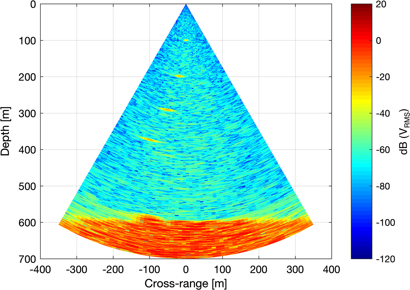
Fig. 9. Reconstructed glacier vertical profile, using a linear 32-element broadside array setup with the separation of virtual antenna pairs set at δ = 1 × λ c, and a theoretical directive beam (HPBW = ±30°).
5. SUGGESTIONS FOR FUTURE DEPLOYMENTS
As with all antenna systems, there exists a tradeoff between gain and beamwidth (Visser, Reference Visser2005); however, correct modifications to the element separation distance (δ) and the number of linear elements (K) will likely improve the imaging quality of both internal layer slopes and the basal topography in future deployments. From our study, we found that δ is itself secondary compared with K. Given the angular swath used in the simulations within this study (±30°), we suggest δ to be roughly equivalent to the central wavelength of the transmitted signal. Doing so will increase the likelihood of constraining internal layer slopes and resolving irregularities in the basal topography. Having the elements too widely spaced risks aliasing the signal returns via the presence of grating lobes (Fig. S2d), while too narrow an element separation reduces the directivity and gain of the signal. (Fig. S2a). Similarly, a higher K value increases the angular acuity and therefore the resulting image's angular resolution (Fig. S3), effectively resolving smaller wavelengths manifested within the bed.
In our simulations (see Appendix), we simplify the scenario by using a linear array with a corresponding bed varying in one direction to reproduce the along-flow section of the ice. As a planar array, similar to our field configuration (Fig. 2a), is simply a series of stacked linear arrays, the number of virtual antenna pairs will either need to be multiplied or the array be towed to create a planar synthetic aperture (e.g. Walford and Kennett, Reference Walford and Kennett1989; Paden and others, Reference Paden, Akins, Dunson, Allen and Gogineni2010) in order to image the bed in two directions to accurately resolve a 3-D representation of the bed roughness. The current version of the pRES unit, which has the capability of switching between up to eight Tx and eight Rx antenna pairs, limits the maximum number of pairs to 64 elements in a planar arrangement, or 32 pairs in a linear arrangement. Therefore, given the current instrument capabilities, there exists a tradeoff between 3-D imaging of internal layer slopes and resolving the basal topography in 2-D. Characterising internal layers in 3-D with a planar setup (e.g. 8 × 8 virtual antenna pairs) can be traded for a maximum-element linear array (32 × 1 virtual antenna pairs) witha higher 2-D resolution to better resolve the bed.
As instrument costs often play a significant factor in the choice of materials used, the ideal antenna would have to be low cost, easily constructed, transportable and robust to withstand the harsh conditions of the polar regions. Additional simulations varying the element factor (Fig. S1) show that the choice of antenna merely limits the width of the usable swath, which is approximately equivalent to its HPBW and exerts no influence over the array factor Eqn (4). The current size of the physical bowtie antennas used in this study (820 mm × 820 mm; Fig. 2a), in addition to their simplicity and low associated costs, have a HPBW of ±80° and were optimised to operate at the air/ice interface. If the antenna size was reduced, a higher frequency would be required to maintain the current antenna properties, which ultimately reduces the range of the system from the internal losses from englacial signal scattering.
6. SUMMARY AND CONCLUSIONS
By tracking the relative range change of internal and basal reflectors, studies involving pRES have demonstrated its potential for measuring vertical strain within ice sheets (Kingslake and others, Reference Kingslake2014, Reference Kingslake, Martín, Arthern, Corr and King2016) and basal melt rates beneath ice shelves (Corr and others, Reference Corr, Jenkins, Nicholls and Doake2002; Jenkins and others, Reference Jenkins, Corr, Nicholls, Stewart and Doake2006; Dutrieux and others, Reference Dutrieux2014; Nicholls and others, Reference Nicholls2015; Marsh and others, Reference Marsh, Fricker, Siegfried and Christianson2016). Here, we describe the use of the instrument with a 16-antenna MIMO array to image internal layers in a fast-flowing outlet glacier that drains a 35 000 km2 catchment on the Greenland ice sheet. The capability of the instrument to measure and partition the movement and slope of internal layers in three dimensions sheds new light on the vertical stratigraphy in a region of complex ice flow, with the potential to greatly improve estimates of vertical velocities and strain rates within such regions. We use a forward model to optimise and improve the angular resolution of the bed echo layer, demonstrating the importance of the array factor to reflect on the specific purposes of the deployment. In addition to its lower power consumption and lightweight, pRES offers novel possibilities when applied in a MIMO configuration.
SUPPLEMENTARY MATERIAL
The supplementary material for this article can be found at https://doi.org/10.1017/jog.2018.54.
ACKNOWLEDGMENTS
This research was funded by the UK Natural Environmental Research Council grants NE/K005871/1 (to PC) and NE/K006126 (to BH and AH), a NASA Cryospheric Science grant NNX16AJ95G (to DMS) and grants from the University of Cambridge Fieldwork Fund and Chung Wei Yi Co. Ltd. (to TJY). We thank Marion Bougamont and Joe Todd for assistance in choosing the field site and ancillary data generated by numerical models; Leo Nathan and Coen Hofstede for assistance in the field; the crew of SV Gambo for logistical support; and Ann Andreasen and the Uummannaq Polar Institute who generously helped and provided local support. PC was the lead PI of the project. Authors are listed according to contribution. The codes for processing the field-collected datasets and the simulation, along with an example dataset, will be submitted to the Remote Sensing Code Library (RSCL; http://rscl-grss.org/about.php) shortly after this manuscript is published. Until that time, the codes and datasets are available by request from the corresponding author.
APPENDIX: EXTENDED METHODS
Synthesised vertical ice section
The model input for our simulation is a synthetic vertical ice section representing an along-flow section of an ice sheet of 800 m × 700 m. Within the vertical section, we introduced several artificial features: (i) four internal layers situated at 100, 200, 300 and 400 m depth along the cross-range centre (x = y = 0 m) with slopes of 0°, 5°, 10° and 15°, respectively, with a uniform reflectivity of −30 dB V RMS at nadir; (ii) a sinusoidal bed situated at a mean depth of 600 m, with π amplitude and spanning 10 wavelengths across the domain, with a uniform reflectivity of −20 dB V RMS at nadir; (iii) A small subglacial topographic feature of 20 m in height and 50 m in width located 100 m off-nadir (equivalent to 9.46°); and (iv) presence of a thick layer of subglacial material situated immediately below the bed layer to the bottom of the section, with an isotropic reflectivity of −30 dB V RMS below the bed layer.
We assume the ice within this section to be homogeneous in composition, resulting in the dielectric properties of ice to be constant through depth and space. Though this is rarely the case, especially in areas of accumulation and/or fast flow, there exists only several profiles of ice composition from ice core records (e.g. Dahl-Jensen and others, Reference Dahl-Jensen, Gundestrup, Gogineni and Miller2003) and this assumption is often necessary, especially when the purpose of the experiment is exploratory, as in this simulation. Therefore, in addition to simplicity, we do not incorporate these additional scenarios into our simulations.
Backscattering coefficient
In order to make effective decisions regarding radar design, we need an expectation of the target's scattering characteristics. Although radar signal propagation through ice incurs increasing attenuation through depth as a result of radiation scattering and absorption (e.g. Plewes and Hubbard, Reference Plewes and Hubbard2001), this simulation assumes no power loss unless the signal interacts with designated layers within the vertical section for simplicity. Here, we characterise the backscattering coefficient σ 0 using a Gaussian distribution with respect to the angle of incidence α, with an incoming beam angle normal to the layer reflecting all power back to the source, and a beam angle perpendicular to the layer reflecting no power back to the source:
 $$\sigma^0 = \beta^0 \gamma f \left( \alpha \right)$$
where β 0 is the radar brightness of the layer, f (α) the distribution as a function of the angle of incidence α, and γ an adjustment factor dictating the spread (variance) of the distribution.
While internal layers are known to be specular reflectors (Drews and others, Reference Drews2009; Holschuh and others, Reference Holschuh, Christianson and Anandakrishnan2014; Cavitte and others, Reference Cavitte2016, Fig. 7a), the ice/bed interface is in most places a diffuse reflector (Drews and others, Reference Drews2009, Fig. 7b) and is often highly variable in specularity (Schroeder and others, Reference Schroeder, Blankenship, Raney and Grima2015; Young and others, Reference Young, Schroeder, Blankenship, Kempf and Quartini2016). Therefore, for the simulations within this paper, the value of γ was set at 1 with respect to receiving the bed echo in the absence of definitive knowledge of the bed, while γ was reduced to 0.025 for internal layers due to their high specularity (Drews and others, Reference Drews2009; Holschuh and others, Reference Holschuh, Christianson and Anandakrishnan2014; Cavitte and others, Reference Cavitte2016).
Antenna beam generation and synthesis
For the purposes of the simulation, the antenna array was treated as a point located at the centre of the domain resting on the ice surface (0, 0) from where the beams are transmitted and received. A virtual beam is emitted from the array point into the ice vertical section as a function of the scanning angle, producing an array factor F a with a field of vision constrained by the antenna's radiation pattern (Eqn 4). The beam then travels through the section at the designated steering angle, of which at each depth step, a proportion of the total energy is reflected back and received by the array through backscatter as a function of the two-way distance from the array.
The received power (P r) for each pixel at a specific distance (d) and angle (θ) from the array is then a combination of the transmitted and received signals (F 2 due to reciprocity) and the resulting backscattering coefficient (σ 0):
 $$P_r \left( \theta,d \right) = F \left(\theta,d \right)^2 \sigma^0 \left( \theta,d \right)$$
Pixels were then synthesised through distance and angle to reproduce the input ice profile.


 Open access