Introduction
Heat exchange over the polar oceans is strongly affected by the way in which short-wave radiation interacts with the ice pack. A quantitative understanding of this interaction is fundamental in treating many large-scale problems involving the ice, the upper ocean, and the atmospheric boundary layer. The short-wave energy exchange is complicated by non-uniformities in the ice cover which cause its optical properties to exhibit large variations in both the horizontal and vertical. During the height of the melt season, for example, a relatively small area in the ice pack may contain leads, thin ice, surface melt ponds, thick white ice, and snow patches, all having significantly different optical properties. An additional complication arises because the surface and internal structure of the ice are modified by the absorption of short-wave radiation. To answer questions regarding the overall mass balance of the ice pack, the amount of energy available for primary production in the upper ocean, latent-heat storage within the ice, or the regional radiation balance, it is necessary to know not only how the various types of ice are distributed in time and space, but also the optical properties of each ice type.
Relatively little information is available regarding the attenuation of short-wave radiation by sea ice. Bulk extinction coefficients describing the total amount of short-wave radiation absorbed within the ice (see Equation (3), p. 453) have been measured in both the Arctic and Antarctic (Reference UntersteinerUntersteiner, 1961; Reference ThomasThomas, 1963; Reference ChernigovskiyChernigovskiy, 1963; Reference Weller and SchwerdtfegerWeller and Schwerdtfeger, 1967; Reference WellerWeller, 1969); the observed values are remarkably consistent, ranging from 1.1 to 1.5 m-1. No spectral data have been reported. Sea-ice albedos (surface reflectances) are considerably easier to measure than extinction coefficients and have been routinely observed as part of most field programs carried out over pack ice. Extensive albedo summaries have been given by Reference MarshunovaMarshunova (1961), Reference ChernigovskiyChernigovskiy (1963), and Reference Bryazgin and KoptevBryazgin and Koptev (1969) for the Arctic ice pack. Quoted albedo values range from 0.20 over some melt ponds to 0.75 over white ice; typical values for melting white ice are 0.60-0.65. Areal averages have been obtained from high towers (Reference LanglebenLangleben, 1968, 1969) and from aircraft (Reference HansonHanson, 1961; Reference Buzuyev, Buzuyev, Shestirikov and TimerevBuzuyev and others, 1965; Reference LanglebenLangleben, 1971), indicating summer values in the 0.30-0.60 range. Long-wave albedo averages have been measured by Reference Bryazgin and KoptevBryazgin and Koptev (1969) in a single broad band between 600 and 1 200 nm, but high-resolution spectral observations have not been made
Because polar snow can undergo such large changes in internal structure, its optical properties span a much broader range of values than do those of the sea ice. For example, field measurements of the bulk extinction coefficient vary from 4.3 m-1 in dense Antarctic snow (Reference Weller and SchwerdtfegerWeller and Schwerdtfeger, 1967) to 40.1 m-1 in fresh snow (Reference ThomasThomas, 1963). Reported albedos range from 0.50 for melting old snow to values in excess of 0.95 for fresh snow, although more typical values lie in the 0.70-0.85 range. Reference LiljequistLiljequist (1956) and Reference ThomasThomas (1963) have measured light attenuation in snow at several wavelengths and have found a fairly steep increase with wavelength out to 650 nm. The albedo of snow, on the other hand, does not appear to exhibit strong spectral variations in the visible. Reference MellorMellor (1965) reported albedos in the 400-700 nm region which show a slight decrease with wavelength, while Reference ThomasThomas (1963) and Reference KondratyevKondratyev (1969) found a slight increase over a similar spectral range. Reference McClatcheyMcClatchey and others (1971) show a decreasing albedo for fresh snow, but an increasing albedo over old snow up to about 650 nm. Above 700 nm, the available data indicate a gradual decrease out to about 1 000 nm, after which the albedo drops sharply to 0.10 at 1 500 nm.
Absorption and scattering within the snow and ice cover are controlled primarily by internal inhomogeneities, of which, both the type and spatial distribution are important. In sea ice, light attenuation is influenced by the amount of entrapped brine (Reference Davis and MunisDavis and Munis, 1973), the air-bubble density (Jaffé, 1960) and the grain size (Reference WellerWeller, 1969); for snow, Reference MellorMellor (1965) has demonstrated that attenuation varies independently with density and grain geometry. The albedo of the ice, which relates directly to the amount of back-scattering, depends most strongly on the internal structure of the near-surface layers. The factors which govern the optical properties of the ice are sensitive to the thermal history of the material, displaying marked variations with season, state of the upper surface, and age of the ice. The goals of the present study are to: (i) determine from field observations how the optical properties of sea ice and polar snow depend on wavelength, (ii) define the normal range of spatial and temporal variations in the optical properties, and (iii) attempt to correlate these variations with changes in the surface characteristics and internal structure of the ice cover.
The Arctic Ice Cover
The Arctic ice pack consists of a central region composed primarily of thick multi-year ice which is surrounded by a zone of thinner seasonal ice. Dynamic motions within the ice pack result in the creation of leads where young ice forms and grows rapidly during the winter months. Typically, 5—10% of the central pack is made up of young ice less than a meter in thickness (Reference Thorndike, Thorndike, Rothrock, Maykut and ColonyThorndike and others, 1975); first-year ice comprises 40-50% of the ice pack at its maximum extent.
Substantial differences exist between multi-year ice and first-year ice which has not undergone a summer melt season. Because of its rapid growth rate, first-year ice entraps large amounts of brine which are concentrated near the top and bottom surfaces of the ice, resulting in a C-shaped salinity profile. During the summer, melt water drains through the ice, flushing most of the salt from the surface layers and also decreasing salinity in the lower part of the ice. The volume of brine contained in the ice, however, depends not only on its salinity, but also on its temperature (Reference UntersteinerUntersteiner, 1961). As a result, the distribution of brine volume in first-year and multi-year ice reflects the marked difference in their salinity and temperature profiles. In addition, internal melting and freezing over several annual cycles causes the vapor-bubble density in multi-year ice to be larger than that of first-year ice. The optical properties of these two types of ice should reflect the differences in brine volume and bubble density.
While the optical properties of the ice cover do change gradually during the winter months, the most important changes occur during the summer melt season. As the snow cover decays, bare ice is exposed and melt-water puddles form over much of the surface. Absorption of short-wave radiation causes a rapid deterioration in the bare ice surface and the formation of a granular scattering layer where the surface is above the local water table. In contrast to the relatively high albedo of the bare ice, melt ponds are low-albedo areas where large amounts of solar radiation are absorbed. Light transmitted through pond-covered ice is the source of much of the energy used by photosynthetic organisms in the underlying ocean (Reference Maykut and GrenfellMaykut and Grenfell, 1975). The albedo and spatial distribution of these melt ponds are major factors in the radiation balance at the surface. Melt ponds reach the maximum extent shortly after the disappearance of the snow, when they may cover upwards of 50% of the ice. Spatially averaged albedos during this period appear to be between 0.40 and 0.45 (Reference LanglebenLangleben, 1971) as compared to the 0.60-0.65 which would be expected if there were no ponds. Following this maximum, pond coverage on perennial ice decreases as some ponds drain and others deepen. Decreasing pond coverage suggests that the regional albedo will tend to increase, however it is not known to what extent albedo decreases in the remaining ponds might counteract this tendency.
Accompanying the albedo changes at the surface are changes in the transparency of the ice caused by internal melting and the resulting increase in brine volume. Internal melting stores absorbed solar energy in the form of latent heat, and represents an important energy sink not usually considered in studies of the Arctic heat balance. Throughout the summer there is a progressive increase in brine volume which tends to lower the extinction coefficient of the ice. This effect is most pronounced beneath melt ponds where brine volumes in the latter part of the summer can exceed even those of young ice. Refreezing of the brine during the fall and early winter gradually releases the latent heat, retarding bottom accretion and the rate at which the ice cools. Both the average albedo and the bulk extinction coefficient of the ice increase during this period.
Field Program
To investigate the optical properties of the major ice categories in the Arctic Basin, surface reflectance and transmission data were gathered at two primary locations. Spectral transmission in first-year ice was measured at about 60 sites near Point Barrow, Alaska from 9 to 20 June 1972. The time period was chosen to cover the transition from a predominantly snow-covered surface to one predominantly covered by melt water; the sites were chosen to provide information on a variety of ice thicknesses and surface types. Four categories of first-year ice were examined : (i) snow-covered ice, (ii) melting white ice (ice whose surface lies above the local water table), (iii) blue ice (ice saturated with, but not covered by, melt water), and (iv) ice covered by melt ponds. At the height of the melt season, shallow ponds covered upwards of 50% of the ice surface, while blue ice comprised much of the remaining area. During the observational period, average ice thickness decreased from 185 to 120 cm, with melting evident on both the top and bottom surfaces. By 21 June the ice had deteriorated to the point where observations could no longer be carried out safely.
During the summer of 1974, a second series of observations were carried out on multi-year ice near Fletcher’s Ice Island (T-3) located in the Beaufort Sea (lat. 84° N., long. 77° W.). Although the primary objective was to study changes in the ice cover induced by melting over an entire summer, the program was also intended to identify differences between first-year and multi-year ice. Spectral albedos were measured at approximately 200 different sites, spanning the available surface types; spectral transmission measurements were made at about 60 different sites beneath bare ice and melt ponds. Several vertical profiles of light attenuation were obtained in the upper 50 cm of the ice. Surface conditions encountered on the multiyear ice differed from those of the seasonal ice near Point Barrow in two basic respects: (i) melt ponds covered a smaller area, but were substantially deeper, and (iii) white ice, rather than blue ice, covered most of the unponded areas due to greater surface relief and better drainage.
Radiation data were collected using two portable spectrophotometers which were specially designed for snow and ice applications. In the first instrument, a 2 m long fiber-optics lightguide was used to transmit light from the interior of the ice to the entrance slit of the spectrophotometer on the surface. Because of its small (3 mm) diameter, the fiber-optics probe could be inserted into the ice to measure the transmitted light with only a minimal disturbance of the natural radiation field. Upward- and downward-looking profiles of light intensity were obtained by excavating a narrow trench in the ice, drilling horizontal holes about 1 m in length at various levels in the wall of the trench, and then introducing the probe into these holes with a suitable orientation. The effect of the trench on the radiation field near the sensors was small. Shading of the trench produced no measurable change in the observed light levels.
A submersible spectrophotometer was also built for in situ measurements under floating ice. This version, except for the recording apparatus, was entirely self-contained and was housed in a cylindrical tube 9 cm in diameter and 60 cm in length. To deploy the spectrophotometer beneath the ice, it was attached to the end of a hinged rod and lowered into the ocean through a SIPRE core hole. The rod was securely clamped in a tripod at the surface, and the support arm then locked into position by means of a lifting cable. The horizontal distance from the core hole to the instrument was about 2 m. By rotating the rod at the surface, it was possible to measure light transmission at several points in an annulus around the core hole. The submersible spectrophotometer was also used above the upper surface to determine albedos.
Both spectrophotometers were designed to measure light intensities in the visible and near-infrared region (400-1 000 nm). Wavelength resolution was 8 nm at 400 nm, decreasing to too nm at 800 nm. This resolution, however, can be substantially improved through the use of deconvolution techniques described in the following section. A complete description of the performance and operating characteristics of these instruments has been given by Reference Roulet, Roulet, Maykut and GrenfellRoulet and others (1974).
Data Interpretation
Because both spectrophotometers have a fairly narrow field of view, they measure radiance (radiant flux per unit projected area per unit solid angle in a specific direction) rather than irradiance (integral of radiance over the hemisphere). The albedo (surface reflectance function) and the extinction (irradiance attenuation) coefficient, however, are defined in terms of irradiance and care must be exercised to interpret the measurements properly. Downwelling and upwelling irradiances at the upper surface were measured directly by placing a cosine collector in front of the objective lens of the submersible spectrophotometer. Downwelling irradiance beneath the ice was estimated by first assuming that the emergent radiation field was isotropic, and then integrating over the hemisphere. Neither method could be used to interpret the profile data taken near the surface, and it was therefore necessary to wait for overcast conditions when the incident radiation was diffuse.
The spectrophotometers required about 30 s to complete a spectral scan. Several scans were made at each site and the results averaged to minimize instrumental noise and smooth out any high-frequency variations in the incident irradiance. Usually, spectrophotometer measurements were supplemented with independent observations of total downwelling irradiance at the upper surface in order to take into account the effects of changes in cloudiness and sun angle.
Spectral broadening due to the finite bandpass of the instruments can lead to significant errors in the shape of the observed spectrum, especially at longer wavelengths where the light intensity drops rapidly and the band-pass is large. An interactive deconvolution technique similar to the method of Reference SzőkeSzőke (1972) was used to minimize these errors. With this technique it was possible to suppress most of the high-frequency noise characteristic of direct methods (Fourier transforms, stepping methods, etc.) and increase the spectral resolution to about 2 nm at 400 nm and 20 nm at 800 nm.
To calculate extinction coefficients from measured irradiances, a model is needed to describe how absorption and scattering affect the radiation field within the ice. The approach most commonly used is to apply the Bouguer-Lambert law which assumes that irradiance decreases exponentially through a homogeneous material of infinite optical thickness. This assumption, however, is not strictly true in the lower part of a sea-ice cover because of differences in scattering between the ice and the underlying ocean. The effects of the lower boundary were taken into account by applying a two-stream photometric model which, except for the boundary conditions, followed the formulation of Reference Dunkle and BevansDunkle and Bevans (1956). The ice was assumed to be a homogeneous, plane parallel slab of thickness h. Upwelling irradiance at the lower surface (z = h) was assumed to be negligible since back-scattering by Arctic Ocean water is extremely small (Reference SmithSmith, 1973). Specular reflection at the surface was assumed to be negligible in comparison to back-scattering by ice granules and by vapor bubbles in the ice, so that it was not included explicitly in the upper boundary condition. With these assumptions, the radiative transfer equations of Reference Dunkle and BevansDunkle and Bevans (1956) have the following solutions:
and
where F↓(z, λ) is the downwelling spectral irradiance, F↓ (z, λ) is the upwelling spectral irradiance, rλ is the volume reflectance coefficient, Kλ is the extinction coefficient, F0 ≡ F↓(0, λ), and C = Kλ h +sinh-1 (Kλ/rλ). Equations (1) and (2) were inverted to obtain Kλ and rλ using a two-dimensional Newton-Raphson iteration scheme.
In the semi-infinite case where h is large and z ≪ h, Equations (1) and (2) reduce to:
and
where α
λ
is the spectral albedo and is numerically equal to ![]() . These equations are equivalent to the Bouguer-Lambert law and were used to analyze profile data taken near the surface. Equations (1) and (2) were used in the analysis of transmission data taken below the ice.
. These equations are equivalent to the Bouguer-Lambert law and were used to analyze profile data taken near the surface. Equations (1) and (2) were used in the analysis of transmission data taken below the ice.
Results
Spectral albedos
To facilitate comparison of the measured albedos, most of the data reported below were taken during overcast conditions when the incident radiation field was diffuse. Occasionally, diffuse albedos were estimated from data gathered on clear days using empirical curves for the dependence of albedo on solar elevation (Reference LiljequistLiljequist, 1956; Reference Ambach and AweckerAmbach and Awecker, 1967). A specular correction based on the Fresnel reflection formulae was also applied when treating the melt-pond data. The total albedo correction was generally no more than 0.05. Typical albedo values are summarized in Figures 1 and 2. Given in the figure captions are albedos determined from: (i) spectrophotometer data integrated between 400 nm and 1 000 nm in accordance with Equation (4), p. 455 (αs), and (ii) simultaneous Kipp & Zonen radiometer measurements (α).

Fig. 1. Spectral albedos observed over snow and melt ponds: (a) dry snow (p = 0.40 Mg/m3), clear sky with haze, a = 0.84, α8 = 0.89; (b) wet new snow (5 cm in thickness) over multi-year white ice, overcast, ice, overcast, αs = 0.85; (c) melting old snow (p = 0.47 Mg/ m3), clear, α = 0.63, αs = 0.73; (d) partially refrozen melt pond with 3 cm of ice, overcast, α = 0.50, αs = 0.55; (e) early-season melt pond (10 cm in depth) with white bottom on multi-year ice, overcast, α = 0.37, α s = 0.38; (f) mature melt pond (10 cm in depth) with blue bottom on multi-year ice, overcast, α s = 0.27; (g) melt pond (5 cm in depth) on first-year ice, overcast, α = 0.21, αs = 0.21; and (h) old melt pond (30 cm in depth) on multiyear ice, clear, αs, = 0.15. Curves m1 and m2 were taken from Reference MellorMellor (1965) and apply to dry snow and wet snow, respectively.

Fig. 2. Spectral albedos observed over bare sea ice: (a) frozen multi-year white ice, overcast, α = 0.72, αs = 0.74; (b) melting multi-year white ice, clear, α = 0.57, αs = 0.69; (c) melting first-year white ice, clear, α = 0.47, αs = 0.54; and (d) melting first-year blue ice, clear, α = 0.24, αs = 0.27.
The results indicate that the magnitude and shape of the albedo curves depend strongly on the amount of liquid water present in the upper part of the ice. The albedo of compact dry snow (Fig. 1, curve a) was high and showed only a weak wavelength dependence. This result is in substantial agreement with the observations of Reference MellorMellor (1965), whose curves for new snow and melting snow bracket our measurements for heavy, wind-packed snow. The albedo of wet new snow (curve b) was about 0.05 less than that of the dry snow at all wavelengths. In the case of melting snow (curve c), the albedo exhibited a definite spectral gradient above 650-700 nm, but was again independent of wavelength in the visible.
The albedo of pond-covered ice (Fig. 1, curves e—h) is characterized by a maximum at short wavelengths and a dramatic decrease between 500 nm and 800 nm. Because the water is relatively transparent at short wavelengths, values below 500 nm are determined primarily by the scattering properties of the underlying ice. The transition zone (500-800 nm) represents a region where the albedo becomes increasingly insensitive to the underlying ice as absorption by the water becomes the dominant factor. Above 800 nm absorption by the water is so large that the albedo is determined only by Fresnel reflection from the surface of the pond. Thus, most of the albedo difference between individual ponds occurs in the visible where it is readily apparent to the naked eye. The highest pond albedos (e.g. curve e) were found early in the season on multi-year ice. The ice below such ponds usually appeared to be whitish or cloudy due to the presence of air bubbles in the near-surface layers. Later in the season, as the melt ponds deepened, the albedos tended to be lower due to increasing brine volume and decreasing bubble density in the ice. Curve f shows the albedo of a mature melt pond with a blue bottom, typical of those found during midsummer. In areas where melt ponds persisted throughout the entire summer, melting within the ice was very large. Brine volumes beneath the old pond described by curve h varied from 20% at a depth of 50 cm to about 55% immediately beneath the ice—water interface; except for open leads, this pond had the lowest albedo of any surface examined.
Because air temperatures frequently drop below freezing during the Arctic summer, the albedo of melt ponds is subject to rapid changes due to the formation of fresh ice on the surface. This ice is thin (< 3 cm) and usually lasts only a few days. The albedo of an ice-covered pond (curve d) is intermediate between that of an open pond and that of multi-year ice.
In contrast to the ponds on multi-year ice (Fig. 1, curves e, f, and h), the shallow, dark blue ponds on the first-year ice near Barrow all appeared to be quite similar in color. The high salinity and relative clarity of the first-year ice yielded pond albedos (curve g) substantially lower than those typically encountered on multi-year ice. Because the first-year ice observations were made early in the melt season before appreciable amounts of solar energy had been stored within the ice, brine volumes were lower than those beneath the old melt ponds and albedos slightly higher. Presumably, if measurements could have been carried out later in the melt season, first-year pond albedos would have shown a continuing decrease analogous to the multi-year ponds.
Bare-ice albedos (Fig. 2) span a range which, to some extent, overlaps both the snow and the melt-pond values. Melting multi-year ice (curve b) is typically bluish-white in color and has a decomposed surface layer a few centimeters in thickness. This layer results from enhanced absorption of solar radiation near the surface, and its optical properties differ from those of the underlying ice. Observations were made to determine how variations in this surface layer affect the albedo. It was found that the thicker the surface layer, the higher the albedo; for the range in surface-layer thicknesses (2-15 cm) encountered during the summer, wavelength-independent albedo changes of up to 0.10 were noted. The albedo of the underlying ice was found to be lower than that of the decomposed surface and to have a steeper spectral gradient above 600 nm. For example, when an 8 cm surface layer was scraped away, the albedo decrease was 0.05 at short wavelengths, increasing to a difference of 0.10 at 1 000 nm. When the surface layer was frozen (curve a), there was a small albedo increase at shorter wavelengths and progressively larger increases above 600 nm. This is consistent with other observations which indicate a decreasing spectral dependence with decreasing liquid-water content.
Two types of bare ice were observed near Point Barrow during the melt season: blue ice which closely resembled the melt ponds in color, and white ice which consisted of a drained layer 5-10 cm in thickness, underlain by clear blue first-year ice. Although the albedo of this white ice (curve c) was similar to that of the melting multi-year ice (curve b) at long wavelengths, there was a large difference between the two in the 400-600 nm band. The lower albedo of curve c was primarily due to a smaller amount of backscatter by the underlying blue ice. At long wavelengths where light penetration is small, the albedo was determined by the properties of the surface layer and not by those of the underlying ice. Thus, the surface layers on the first-year and multi-year white ice appear to have had similar optical properties.
The albedo of blue melting first-year ice (curve d) is low due to the lack of a surface scattering layer. At short wavelengths its albedo is only about 0.10 larger than that of pond-covered first-year ice (Fig. 1, curve g); at longer wavelengths the albedo decrease is more gradual than that of the ponds, but approaches the Fresnel limit near 1 000 nm where the influence of the thin water film becomes important.
Extinction coefficients
When interpreting measurements of transmission through a layer of finite thickness in terms of an extinction coefficient, it must be kept in mind that this represents an averaging process over that layer. For a material which exhibits large vertical variations in attenuation, the vertically averaged extinction coefficient is not a meaningful property which can be applied to general situations. An extreme example would be snow covering a layer of sea ice; even if the optical properties of each layer were constant, the vertically averaged extinction coefficient would depend strongly on their relative thicknesses. Thus, for the extinction coefficients to be useful in a descriptive sense, the material they describe must be relatively homogeneous. In this section we have attempted to identify layers and ice types which are fairly uniform, but whose optical properties are distinct.
To study the properties of the near-surface layers, intensity profiles were taken in the snow and in the ice down to a depth of 50 cm. While the snow appeared to be optically quite uniform, melting white ice was characterized by a rapid decrease in attenuation with depth near the surface. The surface of the white ice consisted of a loose granular layer which was about 5 cm in thickness early in the melt season, increasing to about 10 cm by the end of the summer. Beneath this granular layer was a transition zone where the ice became consolidated. In the multi-year ice the transition zone was usually about the same thickness as the granular layer. In the first-year white ice the transition zone was generally absent because the ice below the granular layer was saturated with melt water. Although brine volume and bubble density in the ice below the transition zone changed with depth, this change was gradual and the ice appeared to be fairly uniform. When the ice surface was at or below the local water table, a granular layer did not develop; however, a weak transition zone was present in the latter part of the summer due to the large brine-volume gradient in the upper half meter.

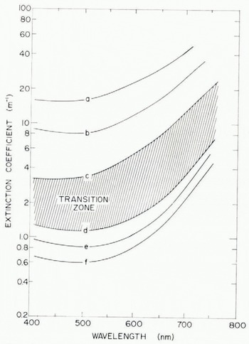
Fig. 3. Spectral extinction coefficients for various types of ice and snow: (a) dry compact snow, p = 0.40 Mg/m3; (b) melting snow, p = 0.47 Mg/m3; (c) surface granular layer (0-5 cm) of multi-year white ice; (d) interior (12-50 cm) of multi-year white ice; (e) first-year blue ice and ponded ice; and (f) ice beneath an old melt pond.
The results shown in Figure 3 point up the large differences in attenuation between the snow (curves a and b), the granular surface layer (curve c), and the interior of the ice (curves d-f). The greatest attenuation was observed in dry, wind-packed snow where the extinction coefficients were roughly 4 times those of the granular layer, and about 20 times those of the interior ice. When the snow began to melt, the density increased from about 0.4 to 0.5 Mg/m3 and the attenuation (curve b) decreased by a factor of 2. Although curve a can be considered representative of dense Arctic snow, the values are probably smaller than those which would be found in the less dense snow more typical of lower latitudes. Extinction coefficients in all cases were relatively constant in the 400-500 nm region, but increased strongly at longer wavelengths. In the red, the spectral gradient of the extinction coefficient was correlated with the magnitude of the total attenuation. The spectral gradient in the snow, for example, was about 2.5 times larger than that in the granular layer and about 9 times larger than that in the interior ice. Spectral gradients in the two snow cases were essentially the same. Extinction coefficients above 750 nm could not be calculated reliably because of the extremely low light levels at these wavelengths.
Extinction coefficients in the surface granular layer were calculated using both upward-and downward-looking intensity profiles and yielded similar results (curve c). Below the granular layer the extinction coefficients decreased rapidly until reaching the interior ice at a depth of 12-15 cm. The range over which the coefficients varied in this transition layer is indicated by the shaded area in Figure 3. The wavelength dependence of the extinction coefficients at a particular depth in this layer was intermediate between curves c and d. Attenuation in the interior ice (curve d) was only about one-third that in the granular layer. The change of intensity with depth in the interior ice is shown in Figure 4. The logarithmic intensity decrease from 12 to 50 cm indicates that the extinction coefficients in this layer were independent of depth at a given wavelength.

Fig. 4. Intensity profiles at selected wavelengths in the interior of multi-year white ice (curve d, Figure 3): (a) λ = 450 nm, Kλ = 1.1 m-1 (b) λ 550 nm, Kλ = 1.2 m-1; (c) λ = 650 nm, =- 2.0 m-1; and (d) λ — 750 um, Kλ = 5.5 m-1. Circles indicate the observed values, and the extinction coefficients are given by the slopes of the lines.
Under-ice measurements were used in conjunction with the profile data to estimate extinction coefficients in the ice below 50 cm. Averaged extinction coefficients in the lower 2 m of the ice were found to be slightly smaller than those immediately below the transition zone; differences of up to 10% were noted. Curve e (Fig. 3) shows averaged extinction coefficients for homogeneous first-year ice calculated from total transmission measurements. Attenuation in relatively clear first-year ice was about 25% less than in the interior of multiyear ice, presumably because of its lower bubble density and higher brine volume. Extinction coefficients in the ice beneath multi-year melt ponds generally decreased throughout the summer in response to internal melting. For example, beneath mature melt ponds in the middle of the summer the extinction coefficients were nearly identical to curve e, but by the end of the summer the values (curve f) had dropped to about 5o% of curve d.
Discussion
Heat-balance calculations involving the ice pack usually employ total radiation fluxes and averaged optical properties. Such an approach, however, can lead to serious errors when estimating heat storage in the ice and energy transmitted to the ocean. This is because horizontal and vertical variations in extinction are neglected and the large spatial differences in albedo not properly taken into account. An additional complication arises because the averaged optical properties depend on the incident spectrum and are therefore influenced by the degree of cloudiness. In this section we examine how these factors affect total energy exchange within the ice, and suggest suitable methods of treating their effects in large-scale heat-balance problems.
Bulk extinction coefficients
Although we have shown (Fig. 4) that the extinction coefficient at a particular wavelength may be constant with depth in an ice layer with uniform physical properties, this does not imply that the bulk extinction coefficient is constant with depth unless Kλ, is also independent of wavelength. In general, the bulk extinction coefficient at a depth Z is given by:

where F z is the total flux at depth z. The magnitude of KZ in a homogeneous layer depends explicitly on the way αλ, Kλ, and F↓(0, λ) vary with wavelength:

where it was assumed that the Bouguer—Lambert law holds at each wavelength.
To evaluate Equation (3), certain assumptions must be made regarding the spectral dependence of αλ, Kλ, and F↓(0, λ) at longer wavelengths because there are significant amounts of solar energy outside the range of our measurements. Under clear skies 25-30% of the incident radiation reaching the surface lies between I 000 and 2 500 nm (Gast, 1960); under cloudy skies there is little energy above 1200 nm and this figure drops to about 6% (Reference Sauberer, Dirmhirn, Steinhauser, österreich, Steinhauser, Eckel and LauscherSauberer and Dirmhirn, 1958). Because of the prevalence of low stratus during the arctic summer, bulk extinction coefficients for the blue first-year ice were determined as a function of depth (Fig. 5) by initially assuming that the incident radiation had a spectral composition similar to that shown by Reference Sauberer, Dirmhirn, Steinhauser, österreich, Steinhauser, Eckel and LauscherSauberer and Dirmhirn (1958); values of αλ and Kλ at long wavelengths were obtained by extrapolation of curve d, Figure 2 and curve e, Figure 3. Near the surface, Kz decreased sharply, dropping by more than an order of magnitude in the first 10 cm. This behavior was due to the strong attenuation at longer wavelengths which caused most of the energy in the red part of the spectrum to be absorbed near the surface. At depths below o cm, most of the remaining energy was contained between 400 and 800 nm.
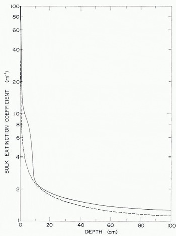
Fig. 5. Bulk extinction coefficients in multi-year white ice (solid curve) and first-year blue ice (dashed curve) as a function of depth under overcast skies. Corresponding extinction coefficients under clear skies are much larger near the surface, but are nearly the same below 5 cm.
Similar calculations were performed to obtain Kz in multi-year white ice (Fig. 5) using a four-layer model which assumed: (i) a granular surface layer 5 cm in thickness with a Kλ given by curve c in Figure 3, (ii) a transition layer 5 cm in thickness with a Kλ which decreased smoothly to the interior ice values (curve d, Fig. 3), (iii) an interior layer 60 cm in thickness where Kλ gradually decreased to 90% of curve d at a depth of 70 cm, and (iv) a homogeneous lower layer where Kλ was independent of depth. Values of αλ above 1 000 nm were based on the results of Reference McClatcheyMcClatchey and others (1971). Near-surface values of KZ in this case were much larger than those in the blue ice, but dropped by a factor of 50 in the first 10 cm to approach the blue-ice curve. Even though Kλ’s in the white ice were much larger than those in the blue ice, the integrated values near to cm were similar because at that level a larger proportion of the energy in the blue ice lay in the 600-800 nm band and, consequently, the integration of Equation (3) weighted K3bb ’s at longer wavelengths more heavily in the blue ice than in the white ice. At deeper levels, relative differences in the spectral composition of FZ for the two cases became smaller, resulting in a gradual divergence of the KZ curves.
When these calculations were repeated for clear sky conditions, it was found that the upper part of the ice absorbed a substantially larger fraction of the total downwelling irradiance. However the decrease in KZ through the upper to cm was even more rapid than in the cloudy case, so that below 10 cm the KZ values were very close to those shown in Figure 5.
Total albedos
The total albedo α depends both on αλ and on the spectral distribution of the incident radiation:

When the sky is clear, α is generally lower because the low spectral albedos at wavelengths above 1 000 nm contribute more strongly to the integral than when the sky is overcast. Equation (4) was evaluated using observed αλ values below 1 000 nm and data on F↓(0, λ) from Reference Sauberer, Dirmhirn, Steinhauser, österreich, Steinhauser, Eckel and LauscherSauberer and Dirmhirn (1958) and Gast (1960); albedos above 1 000 nm were obtained by the methods discussed in the preceeding section. Table I shows total albedos calculated for typical examples of the major surface types. Total albedos for blue ice and melt ponds were found to be about 0.07 larger on cloudy days than on clear days; this difference increased to about 0.14 over white ice and melting snow. Similar calculations were not carried out for dry snow because of the uncertainty in extrapolating αλ for this case.
Table I. Total Albedo as a Function of Ice Type and Cloud Cover

As a check of the overall consistency of the assumptions regarding αx and F↓(0, λ) above 1 000 nm, spectrophotometer data were integrated over wavelength to obtain the bulk albedo αs between 400 and 1 000 nm. αs was then compared with simultaneous measurements of α made with a matched pair of Kipp & Zonen radiometers which had a spectral range of 300-3 000 nm. Assuming that the amount of solar radiation below 400 nm is negligible, the difference between the two values can be written

Thus, Δα is clearly sensitive to the assumptions we wish to test. With the values cited above, Equation (5) predicted that Δα for the melt ponds and blue ice would be 0.01 on cloudy days and 0.05 on clear days; for white ice and melting snow, Δα was 0.02 on cloudy days and 0.11 on clear days. Measured albedo differences (see captions to Figs 1 and 2) for the melt ponds, blue ice, and multi-year white ice agree extremely well with the theoretical calculations, supporting the assumptions used at the longer wavelengths.
Energy absorption in the ice
The amount of energy absorbed by the ice depends not only onKλ , but also on F↓(0, λ) and αλ. In order to separate the effects due to Kλ alone, we first calculated the normalized flux divergence

as a function of depth and wavelength in blue ice and white ice (Figs 6 and 7). Since this normalization defines the net flux at the surface to be unity at all wavelengths, neither the albedo nor the incident flux influences the results. Thus, they apply for both clear and cloudy conditions. The figures indicate that the flux divergence near the surface was larger in the white ice than in the blue ice, regardless of wavelength. Energy absorption by the granular and transition layers, however, was particularly strong in the 600-800 nm region. Because of the large amount of energy lost in the upper part of the white ice, fluxes at deeper levels were substantially smaller than those in the blue ice so that at depths below 10-30 cm (depending on the wavelength), the normalized flux divergence exceeded that in the white ice.

Fig. 6. Per-cent attenuation per cm of the net short-wave radiation at the surface by first-year blue ice as a function of depth and wavelength.

Fig. 7. Per-cent attenuation per cm of the net short-wave radiation at the surface by multi-year white ice as a function of depth and wavelength.
The calculations were then repeated, taking into account the spectral composition of the incident flux and albedo differences between blue ice and white ice. It was found that under clear conditions total energy absorption by the blue ice was 1.7 times that of the white ice; under overcast conditions, this ratio increased to 2.3. Under clear skies, the amount of energy absorbed in the upper 5 cm of the blue ice was about 17% larger than in the surface granular layer of the white ice; this difference increased only slightly (19%) when the sky was overcast. Energy absorption by the white ice decreased rapidly below the granular layer, and at a depth of to cm the flux divergence was only about one-third as large as in the blue ice, regardless of the cloud conditions. Below to cm the flux divergence in the white ice decreased faster than in the blue ice, so that at a depth of too cm the blue ice absorbed 4 times as much energy in the 400-600 nm range and about 7 times as much in the 600-800 nm range.
Although the ratio of absorption in the interior of the blue ice to that in the white ice is relatively insensitive to cloudiness, clouds do, however, have an important effect on the amount of energy absorbed by the ice. The upper 5 cm of the blue ice, for example, absorbed about 38% of the incident short-wave radiation when it was clear, but only about 20% when it was overcast. The upper 5 cm of the white ice also absorbed about twice as much of F 0↓ when it was clear. In addition, F 0↓ is generally much larger on clear days, magnifying the difference in energy absorption at all depths.
Despite the large attenuation and the sharp decrease in KZ near the surface, transmission and absorption within the ice can still be estimated simply using the Bouguer-Lambert law and measurements of net short-wave radiation at the surface. Because KZ decreases slowly below 10 cm, Fz ( z > 10 cm) can be approximated reasonably well from a single vertically averaged extinction coefficient, provided that F 10 is known. F 0 can most conveniently be expressed as a fraction i 0 of the net short-wave radiation at the surface:

The value of i 0 depends both on the type of ice (α λ , Kλ ) and on whether the incident radiation is direct or diffuse. Under cloudy skies, i 0 = 0.35 for white ice and 0.63 for blue ice; under clear skies, i 0 = 0.18 for white ice and 0.43 for blue ice. The decrease in i 0 under clear skies is a result of the greater amount of energy in the infrared, most of which is absorbed in the upper 10 cm.
The Bouguer-Lambert law was used to obtain average extinction coefficients K from calculated values of FZ at 10 and 100 cm. It was found that, below 10 cm, K does not depend strongly on either ice type or cloud conditions. In the white ice, K was 1.5 m-1 under cloudy skies and 1.6 m-1 under clear skies; the corresponding values for the blue ice were 1.4 m-1 and 1.5 m-1. These values are in excellent agreement with those reported by Reference UntersteinerUntersteiner (1961) and Reference ChernigovskiyChernigovskiy (1963), but are about two orders of magnitude lower than the laboratory results of Reference LaneLane (1975). Lane, however, attributes to extinction losses due to surface reflection and backscattering. The magnitude of an “extinction coefficient” calculated in this way depends on the thickness of the sample and therefore is not a fundamental property of the material.
Regional albedos and melt-pond coverage
In order to determine the large-scale radiation balance over the surface of the ice pack, we must know the areally averaged albedo, while to calculate heat storage and light transmission through the ice we need to know the relative areas covered by the different surface types. These two problems are intimately related. Regional albedo information can be gathered efficiently by satellite-borne instrumentation, however, atmospheric absorption complicates such data and knowledge of how the albedo varies with wavelength is needed to interpret the observations. Values of αλ presented thus far can be applied to satellite data only if the surface of the ice pack is relatively uniform, as in the spring and fall when most of the surface is covered with snow. During the summer, however, the large-scale albedo reflects the presence of leads and melt ponds and αλ cannot be represented precisely by any of the curves shown in Figures 1 and 2. In the absence of leads, αλ over the perennial ice can be approximated by a simple combination of average melt-pond and white-ice albedos. Figure 8 shows the dependence of spectral albedos on the amount of area covered by ponds, while Figure 9 shows the corresponding variations in the total albedo a under clear and overcast skies. If the albedo is known in a particular spectral range, the pond fraction can be estimated from Figure 8 and then used in Figure 9 to determine α. Although α λ is most sensitive to pond fraction in the 600-700 nm band, the 400-500 nm band offers the advantages of higher light levels, low atmospheric absorption, and only a weak wavelength dependence for αλ. If the albedo determination is carried out with an instrument having a narrow acceptance angle, specular reflection by the melt ponds will not normally be detected. This is the case with satellite detectors and, therefore, satellites will tend to underestimate albedos and overestimate pond fraction; however, it is still possible to establish the total albedo and true pond fraction from such data. The measured albedo is first used to find an apparent pond fraction from Figure 8, and α is then determined utilizing this pond fraction and the dashed curve in Figure 9, which corrects for the lack of a specular component. The true pond fraction corresponding to the total albedo is then given by the solid line in Figure 9.

Fig. 8. Spectral albedos of multi-year ice as a function of pond fraction when leads are not present.

Fig. 9. Regional albedos over multi-year ice (in the absence of leads) as a function of pond fraction under overcast skies (broken curve) and clear skies (solid curve). If satellite data are used to determine pond fraction, the dashed curve, which corrects for specular reflection from the ponds, should be used to estimate the total albedo.
In practice, the problem is further complicated by the presence of leads which frequently occupy a significant fraction of the ice pack. The albedo of leads is low at all wavelengths, being similar to that of the ponds above 800 nm. Knowing the spectral albedos of each type of surface, the fractional areas covered by leads and melt ponds can be calculated from albedo measurements in two separate wavelength bands. An alternative approach would be to estimate lead area from satellite imagery, and then use this information to compute the pond area with data from a single wavelength band. Once the relative proportions of leads and ponds are known, the total albedo can be found from the equation:
where f p and f l are the fractional areas of ponds and leads, and at, αl, αp, and αl are the total albedos of the three surface types.
Conclusions
While the data presented in this paper have been necessarily limited by the available instrumentation to the 400—1 000 nm range, a substantial part of the solar spectrum lies above 1 000 nm. If the spectral composition of the incident radiation is known, the magnitude of αλ and Kλ above 1 000 nm are not needed for the calculation of heat storage in the interior of the ice or energy input to the underlying ocean because the energy at long wavelengths is absorbed near the surface. On the other hand, if only total radiation fluxes at the surface are known, the above calculations must employ the i 0 approach which requires spectral data above 1 000 nm. Likewise, information on at between 1 000 and 2 500 nm is needed to estimate the surface radiation balance from satellite measurements. The available data suggest that there may be significant differences in the shape of α λ above 1 000 nm for different types of ice and snow, but no systematic study has yet been reported.
A second important question involves the way in which scattering by individual inhomogeneities affects the optical properties of the ice. If scattering functions were known for each type of inhomogeneity, it would be possible to theoretically predict α λ and Kλ from observations of ice structure. However, the complex structure of natural sea ice makes it difficult to isolate the effects of the various inhomogeneities. The field observations, for example, indicated substantial changes in Kλ during the summer melt season as the brine volume increased and the bubble density decreased; melt-pond albedos in the visible also appeared to be directly related to bubble density in the pond bottoms. Unfortunately, brine volume and bubble density are not independent quantities and the field data were insufficient to determine their relative contributions to the observed variations in optical properties. Nevertheless, it seems clear that the magnitudes of α λ and Kλ are largely controlled by the number and size distribution of air bubbles and brine pockets. Thus to understand quantitatively the interaction of short-wave radiation with the ice pack during the polar summer, we must have the ability to generalize the optical properties to take into account changing bubble density and brine volume. On the basis of experience gained during this investigation, it appears that the necessary scattering functions can best be obtained through laboratory experiments where the physical properties of the ice can be carefully controlled and accurately determined.
Acknowledgements
We would like to thank R. Roulet, R. Sprenger, H. LaHore, and F. Rigby for their participation in the field program, and D. Perovich for his assistance with the data reduction. We would also like to thank the Naval Arctic Research Laboratory for the use of their facilities near Point Barrow, and for their logistic support while on T-3. This work was made possible by continued support from the Office of Naval Research, Arctic Program, under Contract N0004-76-C-0234.