Introduction

The Younger Dryas cold episode (12.7–11.5 kyr BP; Reference AlleyAlley, 2000) was marked in the Northern Hemisphere by the expansion of the Laurentide and Fennoscandian ice sheets, and by a partial regrowth of the British ice sheet (Reference SutherlandSutherland, 1984; Reference Mangerud, Shane and CushingMangerud, 1991; Reference MacAyealMacAyeal, 1993). Understanding the evolution of these former ice sheets helps appreciation of contemporary ice masses and their likely behavioural response to future climate-change scenarios. Attempts to reconstruct former glaciers commonly focus on the identification and interpretation of empirical (geological) data within a relatively small area, and permit only local-scale interpretations of glaciers either at their maximum extent or during their retreat. In Scotland this geological approach is complicated by the variable overprinting, reworking or complete removal of landforms relating to the Main Late Devensian ice sheet by those of the much smaller, later, Younger Dryas ice cap (e.g. Reference GolledgeGolledge, 2006). Consequently, geological studies are commonly hampered by their limited ability to accurately constrain marginal contemporaneity, and so struggle to evince details of glacier mass balance or flow characteristics. Numerical modelling of glaciers and ice sheets allows insight into these areas, by simulating ice masses and their governing climates and, most importantly, by enabling the interpretation of glacier evolution through a glacial episode (e.g. Reference Siegert and DowdeswellSiegert and Dowdeswell, 2004). This temporal element is of great importance when trying to identify and differentiate dynamically and climatically forced margin oscillations, and promotes a more complete understanding of the surviving geological record.

Despite the clear benefits of a combined geological and modelling analysis, attempts at numerical simulations of Younger Dryas glaciers in Scotland are relatively uncommon (e.g. Reference Payne and SugdenPayne and Sugden, 1990; Reference HubbardHubbard, 1999), and rarely incorporate explicit field data. In order to address such shortcomings, Golledge and others (2008) presented an empirically validated ice-sheet model for Scotland for the Late-glacial period (15–11 kyr BP). In this paper we aim to:

• 1. Explore the mass-balance regime of the modelled ice cap during its evolution.

• 2. Calculate the balance between flow by internal deformation and flow resulting from basal sliding, and its spatial variability, during the height of the Stadial.

• 3. Calculate the likely pattern of erosion potential of the modelled ice cap and identify areas where greatest basal erosion might occur.

• 4. Predict the spatial organization of subglacial hydrology beneath the ice cap.

• 5. Compare these model results with empirical evidence in western Scotland in order to more confidently link geological features with former glaciological conditions.

The Model

The three-dimensional finite-difference ice-sheet model uses algorithms developed and validated by Reference HubbardHubbard (1999) and Hubbard and others (Reference Hubbard, Hein, Kaplan, Hulton and Glasser2005, Reference Hubbard, Sugden, Dugmore, Norddahl and Pétursson2006). For the experiments presented here, this thermomechanical model uses a domain of 300km × 375 km, with basal topography at 500 m horizontal resolution derived from Intermap’s 1.2 m vertical resolution NEXTMap terrestrial elevation data and British Geological Survey (BGS) 10 m vertical resolution marine bathymetric data.

Mean annual air temperature and mean annual precipitation are calculated from the United Kingdom Climatic Impacts Programme (UKCIP) dataset (Reference Perry and HollisPerry and Hollis, 2005), which provides 5 km resolution data for the entire United Kingdom, interpolated from a national network of 3500 weather stations. Whilst recognizing the benefits of integrating ice-sheet models with Atmospheric General Circulation models (AGCMs), we consider this high-resolution, locally derived UKCIP dataset to be more suitable as input data than climatic parameters derived from the relatively coarse AGCMs, which are more suitable for use in hemisphericscale ice-sheet modelling (e.g. Reference Siegert and DowdeswellSiegert and Dowdeswell, 2004). Use of linear interpolations of climate trends between individual ‘snapshots’ has undoubtedly facilitated greater integration of AGCMs with ice-sheet models, but in some cases such generalization completely removes short-lived climatic events such as the Younger Dryas (e.g. interpolation between time slices at 15 and 9 kyr BP of Reference Charbit, Ritz and RamsteinCharbit and others, 2002). Use of local-scale data is thus preferable for these experiments, but introduces the possibility that quite different model scenarios may result if other climate forcings are used.

An elevation-related positive-degree-day (PDD) scheme drives mass balance by calculating annual accumulation and melt through integration of the snow/rainfall ratio, the amount of refreezing and the net altitude-related snow balance, following Reference Laumann and ReehLaumann and Reeh (1993). Input temperatures are computed using a sinusoidal annual temperature variation fluctuating within a range, and from mean annual temperature, derived from the UKCIP dataset. Precipitation is distributed evenly through the year. Use of a PDD scheme such as this, in preference to a full energy-balance algorithm, is the only pragmatic option where palaeo-data for the latter are lacking (e.g. long- and shortwave radiation balance, wind flux and albedo). We further modify accumulation and ablation patterns by imposing eastward and northward precipitation reductions away from the main ice mass, of 80% and 60%, respectively (Reference Golledge and PhillipsGolledge and others, 2008). Variations in Greenland Icecore Project (GRIP) 20 year resolution δ¹⁸O data (Reference JohnsenJohnsen and others, 2001) are used to define the pattern of temperature fluctuation in the model domain, which is scaled to Scottish palaeotemperatures (Fig. 1) by analogy with modern isotopic values in Greenland (Reference Clapperton and GordonClapperton, 1997). Use of the GRIP temperature pattern as a suitable proxy from Scotland is supported by the close similarity between temperature trends observed in its isotopic variations and those inferred from palaeoecological proxies in the UK (Reference Atkinson, Briffa and CoopeAtkinson and others, 1987; Reference Kroon, Austin, Chapman and GanssenKroon and others, 1997; Reference Brooks and BirksBrooks and Birks, 2000). Furthermore, palaeoglaciological studies in Ireland have established that glacier fluctuations there were broadly consistent with isotopic trends evident in the GRIP record during the Younger Dryas, despite being out-of-phase prior to ∼17 kyr BP (Reference KnightKnight, 2003). Spatial variability of modelled surface temperatures and precipitation inputs across the domain at the height of the Stadial is shown in Figure 2.

Fig. 1. Mass-balance parameter and forcing temperature variability through the Younger Dryas model run, showing (a) fluctuations in rate of annual volumetric change; (b) the 20 year resolution temperature pattern used to force the model run; (c–e) accumulation, annual melt and annual calving volumes, respectively; and (f, g) changes in net volume and areal extent, respectively, of ice in the domain. Note lag between climatic minimum and maximum ice volume.

Fig. 2. Modelled surface temperatures across the domain at 2500 model years and contoured annual precipitation totals. Temperatures incorporate cooling due to altitude; precipitation pattern reflects imposed eastward and northward reductions simulating aridity away from the main ice mass.

Net mass balance, b, is related to the three-dimensional evolution of the ice cap through time, t, through the equation for the conservation of mass, based on the assumption that ice is incompressible:

((1))

where H is ice thickness, t is time, ū is the vertically averaged horizontal velocity and ∇, in this instance, represents the ice flux between adjacent nodes minus surface mass balance. Ice velocity is composed of internal deformation (Reference GlenGlen, 1955), and Weertman-type sliding when basal temperatures are sufficient to generate pressure melting, and is determined through calculation of basal shear stresses corrected by a term for the vertically averaged longitudinal deviatoric stress. The basis and full derivation of this empirically validated ice-stretching algorithm are presented elsewhere (Reference HubbardHubbard, 1999, Reference Hubbard2000, Reference Hubbard2006). Many studies have found that water depth exerts the principal control on the rate of calving at water-terminating glacier margins (e.g. Reference Zweck and HuybrechtsZweck and Huybrechts, 2003). We employ a relatively simple scheme which calculates mass lost due to calving, U _c, as a product of ice thickness, H, water depth, W _d, and a calving parameter, A _c (Reference Brown, Meier and PostBrown and others, 1982; Reference Van der VeenVan der Veen, 1999):

((2))

This crude approximation of calving is clearly less preferable than more complex relationships (e.g. Reference Benn, Hulton and MottramBenn and others, 2007a,Reference Benn, Warren and Mottramb) but is computationally less intensive and is a reasonable solution in our domain, where calving losses are close to zero through much of the model run. Sea level is parameterized at +10m for the duration of the model run, in accordance with empirical sea-level reconstructions for this time period from coastal areas of western Scotland (Reference Peacock, Graham, Robinson, Wilkinson, Gray and LowePeacock and others, 1977; Reference ShennanShennan and others, 1998). Although this parameterization of calving and sea-level altitude has allowed many west-coast glacier limits to be faithfully reproduced by the model (Reference Golledge and PhillipsGolledge and others, 2008), we acknowledge that using different functions and parameter values may have a significant effect on overall ice-cap geometry by locally altering the ablation component of the ice cap’s mass balance. Our domain topography does not include the bathymetry of freshwater bodies, which may also introduce local errors in areas where particularly deep lochs occur (e.g. Loch Lomond).

Thermal evolution of the ice sheet through time, ∂T /∂t, is calculated according to the relationship

((3))

in which k _ice and C _p are the temperature-dependent parameters of conductivity and specific heat capacity, is the three-dimensional velocity vector, ρ _ice is the density of ice and Φ denotes frictional heat resulting from internal strain (Reference HubbardHubbard, 2006).

The model evolves through a 4000 year run from initially ice-free conditions at 15 kyr BP to complete deglaciation by 11 kyr BP. A 0.02 year time-step is used in order to most effectively balance model stability against computation time. The spin-up period of 2000 model years (15–13 kyr BP) prior to the Younger Dryas episode described here (13–11 kyr BP) resulted in intermittent ice growth related to fluctuations in the imposed temperature depression, but almost complete loss of ice from the model domain by 1600 model years. Optimal parameterization was achieved through a series of sensitivity experiments designed to gauge the relative influence of changes in temperature forcing, precipitation distribution and the amount of basal sliding, which are described in detail elsewhere (Reference Golledge, Hubbard and SugdenGolledge and others, 2008). The relative closeness of fit of the numerical simulation to empirical reconstructions through the model run is calculated and logged using a grid-comparison algorithm that compares model outputs against empirical reconstructions in five zones (Reference Golledge, Hubbard and SugdenGolledge and others 2008). This enabled the ‘best-fit’ time slice to be objectively identified where domain mismatch is at its minimum, which was found to occur between 2400 and 2600 model years. In general, outlying icefields reached their maxima earlier than the outlet glaciers of the main ice cap, which showed greater evidence of lags in the transfer of mass through the glacier system (Reference Golledge, Hubbard and SugdenGolledge and others, 2008). Reduction of annual precipitation totals during the Stadial was necessary to control ice-sheet mass balance and to prevent a ‘run-away’ scenario that produced an implausible glacier configuration. Precipitation was reduced by 20% per century from 2500 to 2700 model years, held constant at a 50% reduction from 2700 to 3300 years and returned to normal conditions by increases of 20% per century from 3300 to 3500 years. This artificially enforced aridity during the latter stages of the model run is consistent with inferences from palaeoenvironmental proxies in western Scotland that suggest a drier climate during this period (Reference Benn, Lowe and WalkerBenn and others, 1992). That the resulting simulation closely approximates the distribution of ice cover during the Younger Dryas glaciation in Scotland is demonstrated by the close agreement of modelled maximal ice margins with geologically reconstructed Younger Dryas ice limits (cf. Reference SissonsSissons, 1979; Reference BallantyneBallantyne, 1989, Reference Ballantyne2002; Reference ClarkClark and others, 2004) and concurrence between spatial variations of modelled ice-cap characteristics and interpretations of geological data in the southeast sector of the ice cap (cf. Reference GolledgeGolledge, 2006, Reference Golledge2007a,b; Reference Golledge and PhillipsGolledge and Phillips, 2008).

Model Results

Mass balance

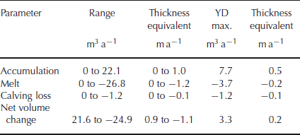
The scaled GRIP-pattern PDD scheme used to drive the mass-balance component of the model couples interpolated horizontal changes in precipitation and temperature across the domain with calculated vertical changes resulting from topography. Figure 1 shows aspects of climatic and glacier evolution through the Younger Dryas model run; Table 1 describes the variability of mass-balance parameters and gives values at the ‘optimum fit’ time slice of 2500 model years. Annual accumulation peaks at approximately +1 m a⁻¹ (Table 1) during the coldest part of the Stadial, from ∼2370 model years, producing a net annual volumetric increase of 21.6 km³ (Fig. 1a). Annual ablation rates achieve a maximum of −1.2 m a⁻¹ (equivalent to a net decrease in volume of 24.9 km³) only a decade later, due to an abrupt (but short-lived) warming oscillation in the GRIP-based temperature curve. Although these extreme values are not subsequently repeated, the lesser peaks evident in Figure 1a, nonetheless, illustrate the sensitivity of the mass-balance model to transient high-magnitude climate oscillations that occur throughout the Stadial (Fig. 1b). Net accumulation through the Younger Dryas (Fig. 1c) integrates losses due to melting (Fig. 1d) and calving (Fig. 1e). Net accumulation is greatest during the short-lived climatic minimum and decreases subsequently as precipitation is reduced, as melting increases (due to the warming climate), and as the ice mass expands to the west coast and calving losses increase. Calving is, however, negligible throughout much of the Stadial, exceeding 1 km³ a⁻¹ only between 2460 and 2540 model years when ten west-coast glaciers are marine-terminating. Figure 1f and g illustrate the integrated consequences of transient mass-balance perturbations through the Stadial, describing changes in total ice volume and total ice extent, respectively. The latter peaks, shortly after the lowest temperatures, are due to the immediate lowering of the climatic equilibrium-line altitude (ELA), whereas ice volume in the domain does not reach its maximum until 2520 model years, 150 years after the thermal nadir. At the ‘optimum fit’ time slice of 2500 model years, the Younger Dryas ice cap exhibits relatively low mass turnover and a net mean thickening of 0.2 m a⁻¹ (Table 1), comparable with current rates in central-northwest Greenland (Reference Johnsen, Dahl-Jensen, Dansgaard and GundestrupJohnsen and others, 1995; Reference DethloffDethloff and others, 2002).

Table 1. Mass-balance parameters through the model run

These results highlight considerable high-magnitude short-term variability in the mass-balance regime of the ice cap during the Younger Dryas, largely due to transient oscillations in the the imposed temperature forcing. The generally positive bias of the mass-balance fluctuations leads to rapid ice-cap growth at the onset of the Stadial, but following the Stadial maximum (2500 model years) the manually imposed enhanced aridity instigates a change to an overall negative mass balance (Fig. 1a). Final ice-cap decay during the closing centuries of the Stadial occurs under reduced precipitation conditions and consistent climatic warming. Deglaciation is more-or-less complete by 3300–3500 model years (Fig. 1f and g), due to overwhelmingly negative net mass balance (Fig. 1a), which results in the loss of ∼1000 km³ of ice in 150 years (Fig. 1g).

Table 2. Parameter ranges, means and variance at optimum fit, 2500 model years

Velocity and flow mechanisms

At the optimum fit time slice of 2500 model years (12.5 kyr BP), surface velocities of modelled glaciers in the domain are commonly >100 m a⁻¹, with some achieving a maximum of ∼550 m a⁻¹ (Table 2). Figure 3a shows the vertically integrated mean-velocity distribution across the ice cap at this time. High velocities in outlet glaciers contrast with much of the interior of the ice cap being relatively static. The maritime icefields on Skye and Mull host zones of relatively fast flow, but eastern plateau icefields (Cairngorms, Monadhliath) are largely inactive. Even within the main ice cap, the majority of faster-flowing ice occurs on the west rather than east. This west–east asymmetry is particularly clearly shown in the differences between the Loch Linnhe area glaciers in the west, and those in the east such as Rannoch Glacier (Fig. 3b and c).

Fig. 3. (a) Mean velocity distribution in the domain at 2500 model years; boxes locate detail areas (b) and (c). (b) Detail of Loch Linnhe area glaciers, showing flow vectors and glacier catchments. (c) Detail of Loch Rannoch area glaciers, showing flow vectors and glacier catchments. Key for detail areas same as (a).

In order to establish such regional contrasts more easily, we calculate catchment-averaged velocities and mean temperatures across the domain (Fig. 4a and b). These summaries integrate surface and basal values at all points within each glacier catchment, and serve to illustrate the dominance of western glaciers in dynamical aspects of the ice cap, in contrast to eastern areas that are colder and flow more slowly. In particular, Figure 4a highlights the importance of Loch Linnhe and Loch Etive as sinks for the largest contiguous area of relatively fast-flowing ice, focusing drainage from mountainous areas both north and south of the Great Glen.

Fig. 4. Model output at 2500 model years showing (a) catchment-averaged velocities across the model domain and (b) catchment-averaged mean temperatures. Note the higher values in western areas in both cases.

From surface and basal ice velocities, V _s and V _b, respectively, it is possible to calculate the proportion of glacier flow that results from basal sliding and from internal deformation (creep) of the ice above the glacier bed. Since surface velocity, V _s, also represents total velocity, which is the sum of basal sliding plus internal deformation, we calculate the velocity due to creep from V _s − V _b, making the assumption that any deformation of ice at the glacier bed will probably result in pressure melting and facilitate sliding, thereby reducing the creep component of basal motion to close to zero. Using this approach we can calculate the relative proportion of flow occurring as a result of each mechanism, by defining the relationship.

((4))

According to this simple relationship, a value of +1 defines areas flowing entirely by creep and −1 areas whose total velocity is accounted for by basal motion, assumed to be sliding. Figure 5 shows the spatial variability of dominant flow mechanisms forecast by the relationship, as well as areas where basal velocities are <1 m a⁻¹.

Fig. 5. Calculated proportions of flow by sliding and by creep, S, within the Younger Dryas ice cap and its outlying icefields, at 12.5 kyr BP, and areas where ice is effectively immobile, with basal velocities <1 m a⁻¹. Note (1) the dominance of internal deformation in central areas of the ice cap, (2) the asymmetry in the width of the marginal fringe of basal sliding and (3) the far more extensive areas of non-sliding ice in the east. Box shows area of Figure 7.

The results show concentric zonation of the ice cap in which creep dominates in the interior of the ice cap, and basal sliding becomes most important nearer the margins. This distribution differs significantly from the pattern of mean velocities shown in Figure 3a, in which relatively fast-flowing radial corridors of ice extend considerable distances into glacier accumulation areas from their ablation-zone termini. West–east contrasts are again evident, clearly illustrated by the marked differences between the icefields in Mull, Skye and Assynt, and in the Cairngorms and Monadhliath, and in the width of the sliding ‘fringe’ around the main ice cap. Sliding is the dominant mode of flow up to ∼20 km up-glacier from western ice margins, and only small areas of immobile ice occur, in the east. However, sliding is only dominant in the lower reaches of outlet glaciers, which are separated from one another by extensive areas of immobile ice. This low-velocity, non-sliding ice is mostly associated with ice divides, interfluves and plateaux (Fig. 5). We do not account for warming of the firn by the release of latent heat from percolation and refreezing of seasonal meltwater, as is reported in many Arctic glaciers (e.g. Reference Trabant and MayoTrabant and Mayo, 1985; Reference Rabus and EchelmeyerRabus and Echelmeyer, 1998), but the possibility nonetheless exists that, by ignoring this process, sliding may be under-predicted in these eastern areas.

Basal processes

The relative ability of ice to erode its bed, E, can be approximated from its basal velocity and the overburden pressure resulting from its thickness, H, so that E = −f | V _b | H, where f is a constant representing bedrock erodibility (Reference Jamieson, Hulton and HagdornJamieson and others, 2008). In order to calculate only the spatial pattern of erosion potential exerted by the ice, rather than the amount of basal substrate eroded, we assume a uniform bed rheology and set f = 1. Figure 6a shows the areas forecast by this formula to be subjected to greatest potential erosion by the Younger Dryas ice cap. The assumption of a uniform bed hardness probably masks the extent of local variability, but at the domain scale the calculated pattern reflects focused erosion along major flowlines within the main ice cap. Due to its dependence on ice thickness, erosion potential is considerably less along glacier margins than beneath their trunks. In these mid-sections of glaciers, elongate zones of high erosion potential occur many tens of kilometres up-glacier from glacier termini (Fig. 6a). Where ice is thin, such as in many of the outlying icefields, the potential for subglacial erosion is negligible.

Fig. 6. (a) Areas exposed to greatest subglacial erosion potential, based on ice thickness and velocity; inset shows detail. (b) Probable subglacial drainage pathways calculated from the glaciohydraulic gradient; inset shows detail. Legend for insets same as for main panels.

Theoretically, where basal ice reaches the pressure-melting point, the meltwater produced will either refreeze, permeate into the underlying substrate or flow along a vector representing the glaciohydraulic gradient. The magnitude of this gradient is largely governed by the thickness of overlying ice and the topography of the glacier bed. Basal meltwater plays a critical role in glacier dynamics, by facilitating sliding where its pressure, P _w, exceeds that exerted by the weight of ice overburden, P _i. As the difference between these two components (the separation pressure, P _s) increases, effective pressure at the ice–bed interface, P _e, decreases and basal sliding is enhanced. The magnitude of this enhancement is limited, however, by increasing bed roughness, since higher water pressures are required to overfill the larger bed cavities, according to the relationship

((5))

where λ is the wavelength of bedrock bumps, τ is the basal shear stress and a is the amplitude of bed roughness (Reference PatersonPaterson, 1994, p. 149).

As we do not calculate melt volumes here, we make the assumption that P _w = P _i and thus that P _s = 0. Under such conditions it is possible to use ice thickness and basal topography to calculate glaciohydraulic gradients at the ice–bed interface. We use ESRI ArcGIS 9.2 flow-accumulation tools to then identify where melt-water would be most likely to accumulate and the direction in which it would flow. Figure 6b illustrates these potential routeways for basal melt-water drainage, based on accumulation within subglacial catchments. Given the dependence on ice overburden pressure it is not surprising that the principal drainage paths flow approximately radially from the thick ice-cap centre to its thinner margins, along the main valleys that also focus the flow of ice. Although weakly developed arborescent drainage networks may occur in some catchment areas beneath the centre of the ice cap, the majority of subglacial meltwater beneath outlet glaciers is predicted to preferentially follow only one dominant path (Fig. 6b), giving rise to a distribution of low-order subglacial streams (Reference StrahlerStrahler, 1952). These hypothetical subglacial streams largely accord with modern drainage networks, due to the high degree of topographic control exerted by the mountainous relief underlying the majority of the ice cap. By simplifying the subglacial hydrology, and by excluding subglacial or ice-marginal lakes, we are able to identify major characteristics of the former ice cap but are unable to provide the spatial detail and accuracy necessary for field comparison. Consequently, this remains a goal for future research.

Discussion and Comparison with Geological Data

The mass-balance data presented here are the first to be calculated for a simulated Younger Dryas ice cap in Scotland at such high temporal and spatial resolution. Such data are valuable both for local palaeoglaciological studies that seek to infer former glaciological conditions from reconstructed ice margins and for studies of contemporary ice caps such as Austfonna, Svalbard, or Devon Ice Cap, Nunavut, Canada, where only remotely sensed or short-term field records are available (e.g. Reference Bamber, Krabill, Raper and DowdeswellBamber and others, 2004; Reference Colgan, Davis and SharpColgan and others, 2008). Additionally, consideration of the mass balance of former ice caps may be useful when assessing the current ‘health’ of glaciers in areas currently experiencing significant changes in their governing climates (Reference DowdeswellDowdeswell and others, 1997) or in better understanding the role of mass balance in influencing glacier response times (Reference Bahr, Pfeffer, Sassolas and MeierBahr and others, 1998; Reference Pfeffer, Sassolas, Bahr and MeierPfeffer and others, 1998). Our results show that glacier inception occurs rapidly under a cooling climate, and that glacierized areas are most widespread more-or-less coincident with the coldest part of the Stadial. This close relation between cooling and area of ice cover is not, however, matched by the pattern of volumetric changes. Integrated glacier volume in the domain reaches a maximum ∼150 years after the climatic minimum, representing a lag in mass transfer through the glacier system as the ice cap endeavours to achieve a state of equilibrium under the fluctuating climate. The possibility that this change in volume–area relationship may be partially influenced by the advection of cold ice towards the glacier bed, stiffening basal ice, as inferred recently in Devon Ice Cap (Reference Colgan, Davis and SharpColgan and others, 2008), is one that may be fruitful to explore in the future. An appreciation of such internally regulated glacier oscillations, representing climatically decoupled thermomechanical feedbacks, may be especially pertinent to the way in which glacier limits and the geological record in deglaciated areas such as Scotland are interpreted.

How glaciers flow excites considerable debate (Reference BoultonBoulton, 1986; Reference Boulton, Dobbie and ZatsepinBoulton and others, 2001; Reference Piotrowski, Mickelson, Tulaczyk, Krzyszkowski and JungePiotrowski and others, 2001, Reference Piotrowski, Mickelson, Tulaczyk, Krzyszkowski and Junge2002; Reference KjærKjær and others, 2006), primarily because of the implications associated with the different flow mechanisms. Whereas widespread deformation of unconsolidated basal sediments may play an important role in glacier motion, it is also clear that basal environments are highly complex and vary in both space and time (Reference Piotrowski, Larsen and JungePiotrowski and others, 2004). Consequently, bed deformation will most likely be accompanied by meltwater-lubricated sliding on rigid beds, as well as flow by the deformation of ice crystals (creep). Whilst our model does not differentiate between basal sliding and deformation of the bed, it allows the balance between basal motion and internal deformation of the Scottish Younger Dryas ice cap to be quantified for the first time. Furthermore, it enables the spatial pattern of this variability to be calculated at 500 m resolution. Figure 5 highlights how flow mechanics are partitioned into concentric zones within the ice cap, reflecting down-glacier changes in basal conditions. From this it may be inferred that deforming beds will only be generated where ice thicknesses and sliding velocities are high, that is, in topographic troughs beneath the ice cap. Accretion of subglacial sediments will occur down-glacier of these areas, where ice is thinner but where it is still sliding and able to transport entrained sediment. Glacier recession will lead to spatial changes in the location of these sediment ‘sinks’, thus the thickest deformable sequences will probably have accumulated at maximal margins with thinner sequences laid down nearer the ice-cap core. These model inferences also imply that, in some central areas, a deforming substrate may have been either completely absent, or patchy, as a result of the very limited sliding that is predicted to have occurred there. Low velocities in the ice-cap core will also have favoured the preservation of pre-existing landscape elements. Transitional areas between non-sliding and sliding ice are likely to have a mixed basal signature. Such areas may host pockets of deformable sediments, partially modified (remoulded) landforms and unmodified relict landscape components.

Geological mapping in the southeast sector of the ice cap has revealed that thick sequences of sediments predating the Younger Dryas are only preserved in topographic hollows near the centre of the ice cap (Reference GolledgeGolledge, 2007a,b) which, according to the modelled flow patterns, coincide with areas of immobile ice on ice divides between divergent glaciers (Fig. 7, ‘1’). Modelled ice divides in this area are also associated with mapped areas lacking thick or widespread Younger Dryas subglacial till (Fig. 7, ‘2’), presumably due to the limited erosion and transport capacity of basal ice in such locations. Disaggregated or streamlined bedrock characterized by metre-scale displacement of blocks (Fig. 7, ‘3’; Reference GolledgeGolledge, 2006) occurs in locations where the model forecasts the down-glacier transition to sliding-dominated ice flow, perhaps reflecting limited transport of basal substrate previously frozen to the glacier bed. Superimposed bedforms showing lineations that cross-cut older features (Fig. 7, ‘4’), are mapped in areas where the model predicts either convergent flow or the onset of flow in tributary glaciers feeding a major outlet, whereas more pervasively streamlined (fluted) bedforms (Fig. 7, ‘5’) are found where modelled ice flow is more substantially dominated by basal sliding, than by creep. Ice-marginal moraines are present throughout the western Highlands, marking successive positions of retreating glaciers. Extensive suites of such moraines thought to represent maximal Younger Dryas glacier limits are shown in Figure 7 (‘6’), adjacent to the sliding termini of discrete outlet glaciers draining the eastern margin of the ice cap.

Fig. 7. The southeast sector of the modelled Younger Dryas (YD) ice cap, showing locations of geological features described in the text, in relation to areas of immobile, sliding-dominated and creep-dominated zones, described in Figure 5. Glacier flow vectors are also shown.

The pattern of greatest erosion potential (Fig. 6a) shows that the greatest work done by outlet glaciers should be concentrated in narrow zones between the core of the ice cap and its margins. Where these zones of high erosion potential coincide with relatively high proportions of flow by basal sliding (Fig. 5) the deforming layer is liable to excavation and mobilization. Fluctuation of glacier margins both through a single glacial episode and over repeated glaciations serves to accentuate these patterns, leading to overdeepened rock basins beneath the mid-sections of outlet glaciers. When the locations of greatest erosion potential forecast by the model (Fig. 6a) are compared with the pattern of rock basins in Scotland identified by Reference SissonsSissons (1967), a striking similarity can be seen (Fig. 8). That these basins extend beyond the modelled Younger Dryas limits, and probably require repeated glacial cycles to develop, may suggest that the ice configuration achieved at the height of the Younger Dryas represents a stage that has been reached many times during repeated Pleistocene glaciations.

Fig. 8. Rock basins in Scotland, modified from Reference SissonsSissons (1967), and their context in relation to the modelled extent of Younger Dryas ice described here. Note the similarity in general distribution to the pattern of erosion predicted in Figure 6a.

The discharge of meltwater beneath glaciers influences their rate of flow by changing effective pressures and basal thermal conditions, seen most dramatically in surge-type glaciers (Reference KambKamb, 1987; Reference MurrayMurray and others, 2000). Understanding the mechanisms of subglacial drainage also greatly assists in the interpretation of the glacial sedimentary sequences (Reference Golledge and PhillipsGolledge and Phillips, 2008), and may help to identify areas where glaciofluvial erosion and deposition are most likely to have taken place. Modelled potential drainage patterns for the maximum Younger Dryas ice cap show that, if P _w = P _i, subglacial meltwater flow may have followed a small number of low-order paths at the beds of individual outlet glaciers. Conduit-type systems are highly effective at discharging meltwater (Reference KambKamb, 1987; Reference PatersonPaterson, 1994) and, by keeping P _w low, maintain high overburden pressures, which to some extent act as a brake on glacier flow. In our simulated ice cap, P _w would most likely have been greatest during deglaciation, due to the considerably increased volume of meltwater generated by the warming climate. This may have reduced effective pressure sufficiently to promote accelerated flow, and possibly even surge-type behaviour amongst some of the outlets, as inferred from geological evidence for Younger Dryas glaciers in Loch Lomond (Reference ThorpThorp, 1991), and the neighbouring outlet in Menteith (Reference Evans and WilsonEvans and Wilson, 2006). The influence of a permeable bed on meltwater pressure and drainage pathways is, however, not accounted for by the model.

Geological investigations north and west of the ice-cap centre have identified landforms indicative of thinner, more dynamic glaciers than those inferred in the south and east (e.g. Reference ThorpThorp, 1986; Reference Bennett and BoultonBennett and Boulton, 1993). These studies have focused on the relative importance of deforming beds to facilitate flow, rather than internal deformation. By identifying the glaciological contrasts evident between different sectors of the ice cap, the model results presented here go some way towards reconciling these apparently opposing views. The higher velocities, warmer beds and greater integrated melting ablation occurring in western areas reflect the former presence of high-turnover dynamic corridors within the ice cap, that drained the central accumulation areas steeply towards a sea level only slightly higher than present (Reference ShennanShennan and others, 1998). East of the main ice divides, however, topographic slopes are considerably lower, and the palaeoclimate was drier. These less-dynamic areas would have experienced less strain heating, raising the effective viscosity of the ice and favouring thicker, more sluggish and probably less erosive glaciers. Whether these thermodynamic contrasts are sufficient to explain the absence of erosional periglacial trimlines in eastern areas, in contrast to their abundance further west, remains an interesting avenue for future research (Reference ThorpThorp, 1986; Reference GolledgeGolledge, 2007a).

Conclusions

Investigation of the mass-balance regime and resultant growth and flow characteristics of numerically simulated Younger Dryas ice masses in Scotland, and their relation to geological evidence, has revealed the following new insights:

1. 1. The modelled ice cap grows rapidly during the onset of the Stadial, and is characterized by extensive but relatively thin ice at the Stadial climatic minimum. Lags in the glacier system result in thickening of the ice cap to reach a maximum domain-averaged thickness at ∼2500 model years.

2. 2. The modelled ice cap is significantly influenced by spatial contrasts in the climate that gives rise to it, so that it is dynamically asymmetric at its maximum, with western glaciers generally warmer and faster-flowing than their eastern counterparts.

3. 3. Flow in the core of the Younger Dryas ice cap probably occurred primarily through ice deformation, enabling the preservation of older sediments and landforms.

4. 4. Basal sliding dominated the flow of western outlet glaciers, and led to relatively thick Younger Dryas sediment accumulations at their margins. East of the ice-cap centre, the modelled ice cover was colder than that in the west, was not sliding at its bed and had very low erosion potential.

5. 5. The geometry of the modelled ice cap favours focused basal erosion in the mid-sections of topographic troughs, and gives rise to a pattern of erosion potential that closely matches many of the locations of mapped rock basins in Scotland.

6. 6. The combined influence of ice-thickness variability and bed topography produces glaciohydraulic gradients that would have preferentially facilitated basal meltwater drainage along low-order glaciofluvial systems, focused into central conduits.

7. 7. Manually enhanced aridity during the latter part of the Stadial, coupled with rapidly rising temperatures towards the end of the Stadial, leads to negative net mass balance and culminates in complete deglaciation around 3300–3500 model years.