


Introduction
Estimates of the current mass balance of the Greenland ice sheet vary in sign and magnitude, as do the potential contributions to the rise in sea level as a consequence of climatic warming (Reference Warrick, Oerlernans, Houghton, Jenkins and EphraumsWarrick and Oerlemans, 1990). Significant glaciodynamic uncertainties are associated with the estimated mass exchange between the Greenland ice sheet and the ocean. Substantial work on this subject has been conducted in West Greenland, including energy-balance modeling (Reference Braithwaite and OlesenBraithwaite and Oleson, 1990), formulation of ablation models (Reference BraithwaiteBraithwaite, 1980) and a mass-balance study of a major outlet glacier (Reference BindschadlerBindschadler, 1984). A key parameter that is poorly constrained is the ablation along the margin of the ice sheet, specifically the calving rate and flux of iceberg discharge from outlet glaciers in northern and eastern Greenland (Reference ReehReeh, 1985, Reference Reeh and Fulton1989). A systematic approach to quantifying basic glaciologic parameters, such as glacier velocities, movement of glacier termini and calving fluxes, would greatly enhance efforts to model accurately the mass balance of the ice sheet and its response to climatic change.
Numerous glaciological studies have used satellite remote sensing to map snow- and ice-facies distributions (Reference Hall, Ormsby, Bindschadler and SiddalingaiahHall and others, 1987, Reference Hall, Chang and Siddalingaiah1988; Reference Orheim and LucchittaOrheim and Lucchitta, 1987; Reference Williams, Hall and BensonWilliams and others, 1991), to detect and measure changes in the positions of glacier termini (Reference DowdeswellDowdeswell, 1986; Reference WilliamsWilliams, 1987; Reference WeidickWeidick, 1995) and spatially quantify ice velocity and shear-stress fields (Reference Dowdeswell and CollinDowdeswell and Collin, 1990; Reference Scambos, Dutkiewicz, Wilson and BindschadlerScambos and others, 1992; Reference Fahnestock, Bindschadler, Kwok and JezekFahnestock and others, 1993; Reference Gotdstein, Engelhardt and FrolichGoldstein and others, 1993; Reference RaneyRaney, 1993). This investigation used Landsat data to describe and quantify characteristics of glacier dynamics for an area in which fieldstudies are logistically constrained.
Objectives
The purpose of this investigation was to develop a set of methodologies with which to map and describe the spatial and temporal variations of tide-water glaciers using remotely sensed satellite data. The methodologies developed for this study were to be applicable to other types of satellite images for the development of consistent base lines of glaciological information For large areas. The specific features that were mapped includD: (1) glacier drainage-basin areas; (2) tide-water glacier-terminus positions; and (3) the derivation ice-surface velocity estimates. A series of cloud-free Landsat multispectral scanner (MSS) and thematic mapper (TM) images of the Kangerdlugssuaq Fjord region in East Greenland was acquired. The criteria for selecting the images used in this study included preference for acquisition dates late in the ablation season, low amounts of cloud cover and the identification of at least one high-quality image to analyze for each year that data were available for the study area. Mass-balance data do not exist for the glaciers in this study area. Similarly, there are no direct measurements of the ice depths, subglacial topography, ice fluxes, calving speeds, calving fluxes, bathymetry of the fjords near the ice fronts or hydraulic characteristics and sediment supply for any of these glaciers.
Study Area
The study area was the Kangerdlugssuaq Fjord region in East Greenland and the extent was defined by Landsat images acquired at path 229, row 12 of the Landsat World Reference System-2 (United States Geological Survey, 1984). The nominal-scene center is at 68° 15′36″N, 31°03′36″ W and covers an area approximately 185 km by 185 km (Fig. 1 and 2). The area is divided into northern and southern domains by Kangerd-lugssuaq Fjord, which is about 75 km long and probably continues as an ice-filled bedrock trough for a considerable distance under the inland ice (Reference BrooksBrooks, 1979). Kangerdlugssuaq Gletscher is one of the largest calving glaciers in East Greenland, with an estimated annual discharge of about 15 km3 water equivalent (Reference ReehReeh, 1985; Reference Andrews, Milliman, Jennings, Rynes and DwyerAndrews and others, 1994). The area south of Kangerdlugssuaq Fjord is completely glacierized to the coast, with most of the ice-free areas restricted to steep slopes. The side walls of Kangerdlugssuaq Fjord and its tributaries are also ice-free. The coastal region northeast of Kangerdlugssuaq (Blosseville Kyst) is composed of Tertiary basalts that extend northward to Scoresby Sund. Ice-free areas increase significantly inland from the coast in this part of the study area. The outer coast is highly glacierized because of high snowfall and low melting as a result of prevalent fogs during the melt season (Reference BrooksBrooks, 1979). The region has widely distributed glaciers, ranging from the large inland ice sheet, small ice caps, large valley and outlet glaciers, and cirque glaciers on the coastal mountains.

Fig. 1. Map of glacier drainage-basin areas delineated from the 2 September 1988 Landsat Τ M image. Numerical annotation of drainage basins corresponds to “index” values shown in Fig. 4 and 5 and listed in Appendix A.

Fig. 2. First principel-component image computed from bands 1–4 of the 2 September 1988 Landsat TM data (scene-id γE22901288246, WRS-2 path 229, row 12).
Image Registration
The images were co-registered and digitally enhanced for photo-interpretation. The 2 September 1988 TM image (scene-id YE22901288246) was used as a reference to which all other images were co-registered. Approximately 15–25 ground-control points were selected from this and each other image in a pair-wise fashion. An independent set of points was selected and used to assess the accuracy of the registration. The root-mean-square error (f.m.s.e) of verification points is a better estimator of the registration accuracy than the r.m.s.e. of the control points used for developing the rectification model. The maximum verification errors from all scene registrations were 38 m in the X and 49 m in the Y directions. These values were then used to develop error estimates in subsequent analyses. Soft-copy digitizing was performed to capture image interpretations directly from the images as map overlays into a geographic information system (Reference DwyerDwyer, 1993).
Delineation of Drainage Basins and Ice Fronts
The 2 September 1988 Τ M image was used to delineate the glacier drainage-basin areas (Fig. 2), the boundaries of which were defined on the basis of topographic divides, divergent flowlines of the glaciers and reference to topographic maps. The glacier-terminus width, defined by the distance transverse to the flow direction and bounded by the lateral bedrock/glacier contacts at the terminus, was measured from this image as well. Because the glacier-basin areas are derived from a single image, the area summaries for glacier basins that extend outside the scene are understated (see Appendix A).
The shoreline and glacier fronts digitized from the 2 September 1988 TM image were used as the compilation base for mapping changes in the glacier-terminus positions, starting with the 1978 MSS image. The coastlines in each image were compared with those digitized from the 1988 TM image to evaluate the local quality of image registration. If the coastlines were congruent and the distance change in terminus positions exceeded the registration-verification errors, then the changes were considered valid. The process of compiling the map of changes to glacier-terminus positions involved overlaying the line-work file compiled from the image acquired at time Tn on to the image acquired at time Tn+1. New ice-front positions were digitized only where changes in glacier-terminus positions were of distances greater than the registration error, thereby suppressing the detection of “false” changes. This approach also avoided the Introduction of misregistration “slivers” that would contribute errors to the summation of areal changes in the glacier terminus.
Quantification of Changes to Glacier-Terminus Positions
The terminus positions delineated from consecutive dates of imagery were used to construct polygons that defined changes in the area of glacier-terminus extent. The polygons were overlain on to one of the two dates of imagery for which changes were being measured to determine the sign of the change. Polygon areas were computed as positive (advance) or negative (retreat) in accordance with the direction of terminus movement. The changes were often irregular across the ice front and numerous polygons resulted from compositing the terminus positions from two dates. A second procedure was used to sum the net area change to the glacier terminus for each glacier drainage basin:

where Aij, is the net area change (km2) for glacier i during time interval j and Pijk is the area of polygon k (k = 1 to n) for glacier i during the time interval j.
The net area changes to each tide-water glacier terminus were plotted as a function of time (Fig. 3). The signs of the net area changes accurately represent the direction of change in the terminus position relative to the previous observation date, but the magnitudes of the changes must be considered static approximations. These plots were used to note episodes and magnitudes of changes to the position of the ice fronts. Intervals with little or no change do not necessarily imply steady-state conditions, because only changes that exceeded the registration error were delineated. Similarly, close inspection of the channel morphology near the terminus positions can identify potential topographic pinning points that would reduce the calving flux and stabilize the position of the ice front (Reference WarrenWarren, 1991, Reference Warren1992; Reference Warren and GlasserWarren and Glasser, 1992).
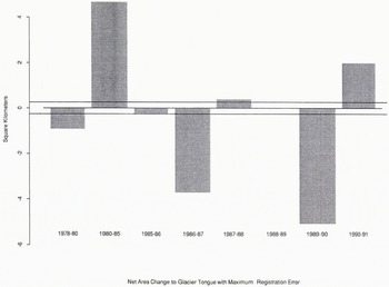
Fig. 3. Bar plot showing the net planimetric area change to the terminus of Kangerdlugssuaq Gletscher. The two solid horizontal lines represent an envelope of the estimated error defined by the product of glacier-terminus width and maximum verification r.m.s.e.
Another parameter used to quantify the magnitude of change to the glacier termini was the normalized linear-distance change:
where Mij is the distance of movement (m) and Ti is the terminus width of glacier i. Approximately 50 of the 75 glaciers in the study area had tide-water ice fronts that could be mapped in all dates of imagery. The ice fronts of tide-water glaciers north of Nansen Fjord were not covered in the 1978 and 1980 images due to offsets in the satellite orbital tracks. Net area changes and normalized linear-distance changes to each of the tidewater ice fronts are summarized in Appendices Β and C.
There were not enough Landsat images to analyze statistically the terminus dynamics using time-series techniques, yet advances and retreats were graphically analyzed to provide a regional perspective of the glacier states. Glaciers were indexed according to their relative location from south (1) to north (75). The net number of advances or retreats of the terminus during the observation period was summarized for each glacier (Fig. 4). The cumulative net area change, relative to the 1978 terminus position for each glacier, is summarized in Fig. 5. This plot shows some marked differences from the plot in Fig. 4, although similar regional characteristics are evident. Kangerdlugssuaq Gletscher, for example, showed more advances than retreats, yet it shows a significant net loss of terminus area during the observation period. The regional trends (dotted lines) in both figures show similar tendencies. Most of the zero-value data points in Fig. 4 and 5 correspond to the land-terminating glaciers for which ice-front positions were not delineated and analyzed for change.
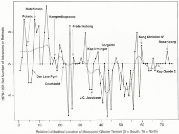
Fig. 4. Latitudinal trend in net number of advances or retreats, relative to 1978, of major tide-water glacier termini. Valuer of X axis correspond to “index” number in Appendix A. The dotted line is the result of non-linear smoothing using running median values.
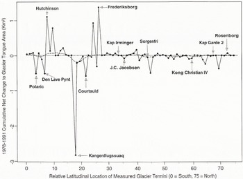
Fig. 5. Latitudinal trend in the net planimetric area change (km2), relative to 1978, of major tide-water glacier termini. Values of X axis correspond to “index” number in Appendix A. The dotted line is the result of non-linear smoothing using running median values.
Estimation of Ice-Surface Velocities
Automated image-to-image correlation techniques increase the efficiency and precision by which digital images can be co-registered (Reference GuindonGuindon, 1985; Reference HannahHannah, 1989; Reference Rignot, Kwok, Curlander and PangRignot and others, 1991). These procedures have also been used to quantify the displacement of spatial features in previously co-registered images for the purposes of target tracking and motion analysis (Reference Emery, Fowler, Hawkins and PrellerEmery and others, 1991). In recent years, however, glaciologists have adapted these techniques to the analysis of ice-surface velocities (Reference Lucchitta and FergusonLucchitta and Ferguson, 1986; Reference Bindschadler and ScambosBindschadler and Scambos, 1991; Reference Scambos, Dutkiewicz, Wilson and BindschadlerScambos and others, 1992; Reference Fahnestock, Bindschadler, Kwok and JezekFahnestock and others, 1993; Reference Lucchitta, Mullins, Allison and FerrignoLucchitta and others, 1993; Reference Lucchitta, Rosanova and MullinsLucchitta and others, 1995). The automated image-correlation algorithm used in this study is based on a fast Fourier transform version of a cross-covariance method (Reference Bernstein, Simonentt and UlabyBernstein, 1983) The procedure implemented for this study is summarized in Appendix D.
The automated correlation techniques were implemented twice. The first case used the 2 September 1988 and 3 July 1989 images and the second case used the 16 July 1988 and the 2 September 1988 images. Twelve of the larger tide-water glaciers in the study area were selected for analysis because crevasse structures were prominent enough to be resolved on the different dates of imagery. The surface velocities were estimated as:
where Vi is the velocity estimated for glacier i, Di is the average displacement (pixels) determined by cross-correlation, 30 is the pixel dimension (m) and Κ is a scale factor used to extrapolate the movement from the period between image observations to an average annual velocity. Similarly, the potential error of the velocity estimates is calculated by:
where E is the estimated error (m a−1), R is the mean r.m.s.e. (pixels) for the verification of image registration and 30 is the pixel dimension (m) The surface-velocity estimates derived from each pair of image cross-correlations are summarized in Table 1. The edited correlation results for Kangerdlugssuaq Gletscher are shown in Fig. 6. The vectors associated with the points indicate the relative magnitude and direction of displacement. Points that were off the glacier surface were eliminated, as were points that had displacement vectors that were not aligned with the direction of ice motion. The latter conditions arise because the algorithm searches for grey-tone correlations and therefore changes in illumination or surface cover result in false radiometric edge displacements.
Table 1. Summary of ice-surface velocities and estimated errors derived using automated image cross-correlation techniques of Reference Scambos, Dutkiewicz, Wilson and BindschadlerScambos and others (1992) and Equation (3) in text


Fig. 6. 16 July 1988 Landsat TM band 4 image with the edited set of image-correlation points and displacement vectors overlain. Note the development of a major fatigue crack oriented transverse to the flow direction.
Discussion
Kangerdlugssuaq Gletscher and Kong Christian IV Gletscher are the largest glaciers in the study area and may be potential outlets draining the inland ice. More accurate delineation of their drainage areas and a higher temporal frequency of analysis of ice-surface velocities and terminus dynamics are needed to determine calving rates. The data analyzed in this study do not allow distinction between floating and grounded tide-water glaciers. The lack of geophysical and field-based measurements precludes definitive statements explaining the mechanisms controlling changes in glacier-terminus positions, although trough geometry and characteristics of the subglacial environment must be important factors.
In general, the glaciers in the southern part of the study area showed a consistent pattern of general advance of the ice-front position and an increase in terminus area, with the exception of Polaric Gletscher. The ice fronts of glaciers at the head of Kangerdlugssuaq Fjord exhibited a net loss of terminus area relative to 1978. Glaciers terminating along the outer coast and in the fjords northward from Mikis Fjord showed small losses to terminus areas. In several cases, adjacent glacier systems exhibit changes that are out of phase with one another, suggesting that glaciodynamic mechanisms unique to floating or grounded ice fronts and topographic controls may be major influences on the terminus dynamics.
No ground-based measurements are available to corroborate the estimates of glacier-surface velocities derived from image correlations, although steady-state mass-balance calculations (Reference ReehReeh, 1985; Reference Andrews, Milliman, Jennings, Rynes and DwyerAndrews and others, 1994) suggest a velocity in the ablation zone of Kangerdlugssuaq Gletscher of ~5.0 km a−1 and the results from autocorrelation of crevasse displacements Table 1) support this estimate. At Kangerdlugssuaq Gletscher, the difference in crevassing and deformation between 2 Septemher 1988 and 3 July 1989 images yielded only a few correlation points, whereas autocorrelation of the two 1988 images yielded a larger set of consistent vectors. In the absence of field-based validation of the ice-surface velocity estimates derived using the image-correlation procedures, confidence in these velocity estimates can only be weighed in terms of the number and distribution of correlation points and/or the repeatability of the results using additional imagery. If reliable parameters can be formulated for balance-velocity models (Reference ClarkeClarke, 1987), then it would be possible to assess the stability of the glacier fronts in the context of the theoretical balanced state of the glacier systems. Furthermore, the derivation of velocity estimates at several times during the year would provide insight to the seasonal variations of ice velocities with implications to the basal hydraulic system (Reference Echelmeyer and HarrisonEchel-meyer and Harrison, 1990).
Automated image-correlation procedures also enable examination of the spatial vanability of estimated surface velocity across a given glacier. For example, surface velocities at the margins of glaciers are measurably lower than in the midstream areas because of friction along the glacier-channel side walls or along the bottom where the ice is thinner. The low velocities of tributary glaciers at the confluence with Kangerdlugs-suaq Gletscher are attributed to the back pressure and shearing due to the higher rate of movement and greater mass of Kangerdlugssuaq Gletscher. Frederiks-borg Gletscher moves faster at the midstream areas up-glacier compared to velocities estimated farther down the glacier. This decrease in velocity was derived from an arm of the glacier downstream from a bifurcation of the glacier tongue before it reaches the fjord. The midstream velocity at Sorgenfri Gletscher is lower than those of Frederiksborg and Kong Christian IV Gletschers but this phenomenon may be a function of the lower mass exchange that occurs in a smaller glacier basin.
Since the rates and patterns of frontal change are determined by the sum of calving speeds and ice velocities, which in turn are responsive to mass flux, ice fronts stabilized by trough geometry will exhibit stepped responses to climatic forcing (Reference WarrenWarren, 1992; Reference Warren and GlasserWarren and Glasser, 1992). The distinction between glaciodynamic and glacioclimatic processes requires longer-term, higher temporal frequency, observation periods than this study able to address.
An understanding of the seasonal variation in ice velocity and the position of the ice front would enable an estimate of the calving rate. Satellite- or aircraft-altimetry data and ground-penetrating radar, combined with the higher temporal frequency observations cited above, would enable determination of ice thicknesses, surface slope and surface roughness (crevassing) of the larger glacier systems. This information is requisite to the development of calving models and characterizing the flow dynamics along the length of the glacier. A question that remains is whether mechanisms and feed-backs of the “Jacobshavn effect” (Reference HughesHughes, 1986) are active for the larger outlet glaciers in East Greenland.
The relationship between climate, mass balance, glaciodynamic response and frontal changes (Reference WarrenWarren, 1991, Reference Warren1992) cannot be addressed with the limited amount of information available. Numerous factors influence the variable response times to changes in mass input to the glacier system (accumulation, feeder glaciers, distributaries), calving dynamics and topographic controls (Reference WarrenWarren, 1992; Reference Warren and GlasserWarren and Glasser, 1992). It appears that several of the large ice fronts are situated at stable positions (channel narrowing, bends, bifurcations, bedrock shelves) where the ice velocity is balanced by the calving rate.
Summary
Landset MSS and TM data can he used to map and quantify changes to glacial features of interest. Glacier drainage-basin areas were delineated and quantified within the geographic area covered by available images. The positions of tide-water glacier termini were mapped and the changes in termini surface areas were quantified. The variations in the positions of glacier termini were plotted and an envelope of potential error was estimated based on the terminus width and maximum image-to-image registration error. Geographic and temporal trends in the changes to tide-water glacier-terminus areas indicated three general domains of glacier statD: tidewater glacier ice fronts in the area south of Kangerdlugs-suaq Fjord exhibited a net advance; the termini of glaciers at the head of Kangerdlugssuaq Fjord exhibited states of advance but an overall loss of terminus area relative to 1978; and most glaciers along the coast and north of Ryberg Fjord showed little change or slight loss of terminus area relative to 1978.
The results from analysis of available Landsat images provide some insights to the state of individual glaciers, although a series of images with greater temporal frequency through the summer, and for several years duration, is required for more rigorous characterization of the glaciodynamic behavior. Indexing of glacier locations is a means of analyzing the types and magnitudes of change in glacier-terminus positions with respect to the geographic distribution and size of glacier basins. Additional information, such as quantification of glacier drainage-channel morphometry and the total area of glacierized basins, would be useful for further characterizing domains of glaciodynamic behavior within the study area. The magnitude of net area or distance change to the tide-water glacier-terminus positions are static estimations and the accuracy with which changes to the ice fronts are quantified can be stated in terms of the amount of potential error attributable to the image registration.
The glacier-surface velocities that were estimated using automated image-correlation techniques are firstorder approximations. Confidence in these estimates grows as the number of displacement vectors with high correlation strength increases. The potential error of the estimated velocities was determined using the verified r.m.s.e. of registration for the image pairs that were used. No field measurements are available with which to corroborate the velocities derived in this study, yet properly constrained balance-velocity models may provide a basis for comparison. Glaciers with the higher surface velocities correspond to the larger drainage-basin areas where commensurately higher rates of mass exchange would be expected. The methodologies developed for this study are applicable to glaciological studies in other areas where a sufficient number of images are available and where the logistics for field studies are seriously constrained. The increasing availability of satellite remotely sensed data, especially synthetic aperture radar (SAR) data, will provide opportunities for monitoring glacier systems on a regular periodic basis. SAR data offer particular advantages in that image acquisitions are not constrained by cloud cover or solar-illumination conditions.
Acknowledgements
This work was performed under U.S. Geological Survey contract 1434-92-C-40004 and as part of a M.Sc. thesis through the Department of Geological Sciences and the Institute for Arctic and Alpine Research at the University of Colorado-Boulder. I should like to recognize the U.S. Geological Survey’s EROS Data Center, TGS Technology, Inc. and Hughes STX Corporation for providing the opportunity and support to undertake this research. I should also like to acknowledge grant DPP-92-24254 for assistance in defining some of the research questions that were addressed in this study. Dr J. T. Andrews and Dr R. S. Williams, Jr provided critical reviews and valuable comments during preparation of the manuscript.
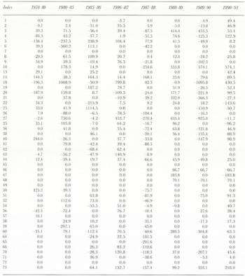
Appendix A
Table 2. Summary of selected glacier drainage-basin characteristics. Glacier names are not official Grønlands Geologiske Undersøgelse designations but rather are taken from local geographic features noted on the 1:250 000 scale topographic maps produced by the Geodetic Institute of Copenhagen. Ice front widths are not reported for glaciers that terminate on land

APPENDIX B
Table 3. Summary of the observed planimetric area change (km2) to tide-water glacier termini (in km2)
APPENDIX C
Table 4. Summary of normalized linear distance change to tide-water glacier termini (in m)
APPENDIX D
A number of small image chips (square blocks of contiguous pixels) were extracted from a reference image and matching chips were sought in a larger area within a second (search) image. The reference and search chips were compared at every center-pixel location in the search area for which the reference chip fitted entirely. The brightness values for pixels within the chips were compared pixel by pixel and the similarity between the reference and search-area chips was quantified by a measure of correlation intensity that was used to construct a map of correlation strength. A detailed discussion of the algorithm has been presented by Reference Scambos, Dutkiewicz, Wilson and BindschadlerScambos and others (1992). The search-chip size was specified to be 128 by 128 pixels, the reference chip was 64 by 64 pixels and the grid spacing for positioning the chip centers was specified to be at 15 pixel intervals in the line and sample direction. The grid spacing determines the number of attempted matches so that, if the grid spacing is reduced by a factor of 2, the number of attempted matches increases by 4. In general, large search and reference chips tend to produce larger strengths of correlation for a given region of the image. Several statistical measures of the correlations were computed for each grid point that is centered within the reference chip. The correlation results were edited by graphically displaying one of the images with the grid points overlain. Points for which an acceptable correlation strength was achieved or that had small estimated X and Y errors were used for estimating the surface velocity. Large crevasses that exhibit translational movement yield the best displacement vectors.


